Evolution of dwarf galaxy observable parameters

Abstract

We present a semi-analytic model of isolated dwarf galaxy evolution and use it to study the build-up of observed correlations between dwarf galaxy properties. We analyse the evolution using models with averaged and individual halo mass assembly histories in order to determine the importance of stochasticity on the present-day properties of dwarf galaxies. The model has a few free parameters, but when these are calibrated using the halo mass - stellar mass and stellar mass-metallicity relations, the results agree with other observed dwarf galaxy properties remarkably well. Redshift evolution shows that even isolated galaxies change significantly over the Hubble time and that ‘fossil dwarf galaxies’ with properties equivalent to those of high-redshift analogues should be extremely rare, or non-existent, in the local Universe. A break in most galaxy property correlations develops over time, at a stellar mass $M_{*}\simeq 10^{7}\,{\rm M_{\odot}}$. It is caused predominantly by the ionizing background radiation and can therefore in principle be used to constrain the properties of reionization.

1 Introduction

Studies of galaxy evolution in cosmological context usually focus on massive galaxies ($M_{*}>10^{9}\,M_{\odot}$) instead of dwarf galaxies because the latter are much harder to detect and study observationally due to their low luminosities (e.g., Vogelsberger et al., 2014; Schaye et al., 2015). However, with increasing amount and quality of data the interest in dwarf galaxies also increases. They are scientifically interesting and important because their evolution depends on cosmological structure formation on the smallest scales and so in principle their observed properties could be used to test cosmological models in this still weakly constrained regime. For example, research on dwarf galaxies could help illuminate the nature and properties of dark matter (Lovell et al., 2014). However, galaxies are highly non-linear systems and so a solid theoretical understanding of their evolution is needed to answer such questions. This is especially true for dwarf galaxies as their evolution is highly sensitive to complex baryonic matter processes due to their shallow gravitational potentials (e.g., Pontzen & Governato, 2012; Brooks et al., 2013; Sawala et al., 2015).

In recent years, a lot of progress has been achieved in understanding dwarf galaxy properties and evolution. Cosmological-scale representative volume simulations now reach baryonic mass resolutions $M_{\rm res}<10^{5}{\rm M_{\odot}}$, while zoom-in simulations reach $M_{\rm res}\sim 30{\rm M_{\odot}}$ (Wheeler et al., 2019), which allows investigation of galaxies with virial masses in the range $10^{7}{\rm M_{\odot}}<M_{\rm vir}<10^{10}{\rm M_{\odot}}$ (Wang et al., 2015; Munshi et al., 2017; Wheeler et al., 2019). These simulations reproduce stellar-halo mass relations that are consistent with observational data (Munshi et al., 2017; Garrison-Kimmel et al., 2019). Star formation in the smallest galaxies is truncated by reionization (Efstathiou, 1992; Thoul & Weinberg, 1996; Dijkstra et al., 2004; Hoeft et al., 2006; Dawoodbhoy et al., 2018; Wheeler et al., 2019), but even these galaxies should build up stellar masses $M_{*}\sim 10^{3}{\rm M_{\odot}}$ before being quenched (Ricotti & Gnedin, 2005; Wheeler et al., 2015; Munshi et al., 2017), although this result is sensitive to the star formation prescription used (Munshi et al., 2019). More massive dwarf galaxies have bursty star formation histories (SFHs) (Wheeler et al., 2019; Garrison-Kimmel et al., 2019), consistent with observations, and are predominantly quenched by stellar feedback (Wang et al., 2015), although supernova feedback alone might not be able to quench them completely (Bermejo-Climent et al., 2018; Smith et al., 2019). Differences in merger histories lead to a spread in final galaxy parameter distributions, with more massive and larger galaxies forming when the halo assembly history is dominated by minor, rather than major, mergers (Cloet-Osselaer et al., 2014).

Observational campaigns allow investigation of individual dwarf galaxies down to the level of individual dense cores (Rubio et al., 2015) as well as examination of their populations. These campaigns focus on nearby galaxies, i.e. satellites of the Milky Way (Newton et al., 2018; Muñoz et al., 2018) or Local Group members (Drlica-Wagner et al., 2015), with the MADCASH survey being an exception (Carlin et al., 2016). Another recent important result is the discovery of seven galaxy groups composed purely of dwarf galaxies (Stierwalt et al., 2017), confirming theoretical predictions that primordial density fluctuations should be scale-free and that in some cases, dwarf galaxy populations can evolve in a similar way to their more massive counterparts.

Such observations reveal numerous statistical correlations between various galaxy parameters. In the case of massive galaxies, these can be described by simple power-laws throughout wide parameter intervals (e.g., Finlator & Davé, 2008; Elbaz et al., 2011). Dwarf galaxies may also follow these correlations; however, because they might be significantly affected by processes which are not very important for massive galaxies, there might be a deviation at low masses from simple power-laws in these relations which might yet be detected by future surveys. There is some evidence for this deviation in, for example, the star-forming main sequence (McGaugh et al., 2017) and the mass-metallicity relation (Blanc et al., 2019). One process which might create this deviation is heating by the intergalactic radiation field (Barkana & Loeb, 1999). During the epoch of reionization the average temperature of intergalactic gas rapidly increases up to $\sim 2\times 10^{4}$ K (McQuinn et al., 2009), which is above the virial temperature of halos with masses lower than $\sim 10^{10}\,M_{\odot}$. Gas accretion in these halos therefore should be shut-off and the star formation rate (SFR) should rapidly decrease (Gnedin, 2000; Dawoodbhoy et al., 2018; Ivkovich & McCall, 2019).

In this work we use a semi-analytic model of dwarf galaxy evolution to study how, in the standard $\Lambda$CDM cosmology, the statistical relations between various galaxy parameters at the low-mass end depend on cosmological redshift, and how these relations are affected by the stochasticity of the dwarf galaxy halo mass assembly. We calibrate some free parameters in the model using the stellar mass - halo mass relation and stellar mass-metallicity relation. Our model reproduces the observed galaxy stellar mass - gas mass relation and the stellar mass - SFR relation very well, and approximately reproduces the observed gas metallicities. Redshift evolution of these relations shows that even isolated galaxies change significantly and ‘fossil dwarf galaxies’ left over from the early Universe should be extremely rare. We also predict a break in most galaxy correlations at stellar mass $M_{*}\sim 10^{7}\,{\rm M_{\odot}}$. This is consistent with observations, although data for isolated dwarf galaxies with $M_{*}<10^{7}\,{\rm M_{\odot}}$ is scarce. Our results will be testable with near-future observations and should help better interpret their results.

The paper is organized as follows. In section 2 we describe the semi-analytical model, in section 3 we decribe the calibration of the free parameters. The main results - analysis of observable parameter evolution and importance of stochastic mass assembly - are presented in section 4. Finally, we discuss our results in the context of cosmological structure formation, provide predictions for forthcoming surveys, and analyse the various assumptions made in the model in section 5. We conclude in section 6.

Throughout the paper, we assume a standard $\Lambda$CDM cosmology with cosmological parameters $H_{0}=67.74\,\mathrm{km}\,\mathrm{s}^{-1}\mathrm{Mpc}^{-1}$, $\Omega_{\mathrm{b}}=0.05$, $\Omega_{\mathrm{m}}=0.31,$ and $\Omega_{\Lambda}=0.69$ from Planck Collaboration et al. (2016).

2 Description of the model

The semi-analytic model used here is very similar to the one we used in Ledinauskas & Zubovas (2018, hereafter Paper I). We therefore present it only briefly, focusing mainly on the changes made and refer the reader to Paper I for more detailed explanations.

We assume that dwarf galaxies are composed of 3 main components: a dark matter halo, a gas disk and a stellar disk. In the subsections below we describe the equations which are used to track the evolution of these components in time. We use two versions of our model. In the first version, the mass growth of dark matter halos and the merger rates are calculated by using the average fitting formulas from cosmological N-body simulations (section 2.1). In the second version we use individual dark matter halo merger trees (section 2.2). The first version is used to calibrate the free parameters and study the average galaxy evolution trends and their average parameters while the second version is used to study the effects of different possible mass growth histories. Hereafter we call the first model ‘average’ and the second ‘stochastic’.

2.1 Dark matter halo mass growth

The formation of dark matter halos, their mass assembly histories (MAHs) and merger rates have been studied in detail with N-body simulations and there are various fitting formulas that approximate these processes rather well. In the average model we use a fitting formula for dark matter halo mass growth rate from Fakhouri et al. (2010):

$$\frac{\langle\dot{M}_{\rm dm}\rangle}{{\rm M_{\odot}}\,{\rm yr}^{-1}}=46.1\left(\frac{M_{\rm dm}}{10^{12}\,{\rm M_{\odot}}}\right)^{1.1}\left(1+1.11z\right)\sqrt{\Omega_{\rm m}\left(1+z\right)^{3}+\Omega_{\Lambda}},$$ (1)

where $M_{\rm dm}$ is the dark matter halo mass. This equation is appropriate for dark-matter-only simulations. The halo mass function in simulations including baryons shows that the total abundance of halos of a given mass is $\sim 25\%$ lower; this also means that the mass of halos with a given abundance is $\sim 25\%$ lower (Sawala et al., 2015; Munshi et al., 2019). We tested the importance of this effect by rerunning the average models with a dark matter halo growth rate reduced by $25\%$ and found that this makes almost no difference to our results.

Two processes grow the dark matter halo mass: smooth accretion from intergalactic medium (IGM) and merging with other halos. The average rate of mergers with halos of a given mass is calculated by using the fitting formula from Genel et al. (2010):

$$\frac{\mathrm{d}^{2}N_{\rm merg}}{\mathrm{d}\omega\mathrm{d}x}=AM_{12}^{\alpha}x^{b}\exp\left((\tilde{x}/x)^{\gamma}\right)\,,$$ (2)

where $N_{\rm merg}$ is the average number of mergers for a single halo, $\omega$ is the monotonic function of time which can be used as a natural time coordinate in Press–Schechter theory (the precise definition and approximate formula for it can be found in Neistein & Dekel, 2008), $x$ is the ratio between the larger and smaller halo masses, $A=0.065$, $\alpha=0.15$, $b=-0.3$, $\tilde{x}=2.5$, $\gamma=0.5$ are fitted free parameters, $M$ is the sum of the masses of the two halos. This relation fits both pure N-body simulations as well as results of the Illustris simulations that include baryonic processes (Rodriguez-Gomez et al., 2015).

2.2 Merger trees

To get the merger trees of individual halos for the stochastic models, we used the publicly available code Pinocchio (Monaco et al., 2013) which is based on the Lagrangian perturbation theory. Like in Paper I, we used a run with box size $d=28$ Mpc, sampled with $800^{3}$ particles. We assumed that the minimal halo comprises 10 particles, which is standard value for Pinocchio. This translates to the smallest halo mass $M_{\rm min}\approx 2\times 10^{7}\,M_{\odot}$ which is small enough to resolve the merger trees of halos with the final mass $M_{\rm dm,0}\geq 10^{9}\,M_{\odot}$. As a result, this is the lowest present-day mass of halos for which we have stochastic models.

Also like in Paper I we used only halos which are isolated throughout their whole lifetime. We define a halo as isolated if it is farther than $2r_{\rm vir}$ from all other more massive halos throughout the Hubble time, where $r_{\rm vir}$ is the virial radius of the more massive halo:

$$r_{\rm vir}=\left(\frac{3M_{\rm dm}}{4\pi\rho_{\rm crit}\Delta_{\rm vir}}\right)^{1/3}\,,$$ (3)

where $\rho_{\rm crit}$ is the critical density of the Universe and $\Delta_{\rm vir}$ is the overdensity of the collapsed and virialized spherical top-hat density fluctuation, which we calculated by using fitting formula from Bryan & Norman (1998).

After running the Pinocchio simulation, we selected subsets of halos with final masses $M_{\rm dm}\left(z=0\right)\simeq 10^{9}\,{\rm M_{\odot}}$, $2.5\times 10^{9}\,{\rm M_{\odot}}$, $5\times 10^{9}\,{\rm M_{\odot}}$, $10^{10}\,{\rm M_{\odot}}$ and $5\times 10^{10}\,{\rm M_{\odot}}$. We chose a small mass interval around each value that included $N_{\rm h}=300\pm 10$ halos, leading to $1500$ stochastic model halos in total.

2.3 Dark matter halos

Properties of dark matter halos are handled identically to Paper I. Their density is assumed to follow the Navarro-Frenk-White (NFW) profile (Navarro et al., 1996), truncated at the virial radius. The concentration parameter, which is defined as the ratio between virial radius and NFW scale radius, was calculated by using the model of Zhao et al. (2009), which relates the concentration parameter $c$ to the time $t_{0.04}$ at which the halo assembled 4% of the mass it has at time $t$:

$$c(t)=4\left[1+\left(\frac{t}{3.75t_{0.04}}\right)^{8.4}\right]^{1/8}.$$ (4)

We characterize the gravitational potential of the dark matter halo by its maximum circular velocity, which for the NFW profile can be calculated by

$$v_{\rm max}\approx 0.465r_{\rm s}\sqrt{4\pi G\rho_{0}}\,$$ (5)

where $\rho_{0}$ is the normalization density of NFW profile.

2.4 Gas accretion and cooling

Similarly to dark matter, the gas mass of a galaxy increases because of accretion from the IGM and mergers with other galaxies. Like in Paper I, we assume that before the epoch of reionization smooth accretion of gas is proportional to smooth accretion of dark matter:

$$\dot{M}_{\mathrm{g,acc}}=\langle f_{\mathrm{b}}\rangle\dot{M}_{\mathrm{dm,acc}}\,,$$ (6)

where $\langle f_{\mathrm{b}}\rangle\approx 0.19$ is the ratio between the average densities of baryonic and dark matter in the Universe.

We also use the same algorithm as in Paper I to calculate the effect of heating by the photoionizing intergalactic radiation field during and after the epoch of reionization. This algorithm was first proposed in Okamoto et al. (2008). If the virial temperature of a halo is lower than the average temperature of intergalactic gas at overdensities $\Delta_{\rm vir}/3$, then smooth accretion of baryonic matter is shut off. If the virial temperature is lower than the intergalactic gas temperature even at overdensities higher than $\Delta_{\rm evp}=10^{6}$, the gas of the galaxy is evaporated exponentially:

$$\dot{M}_{\mathrm{evp}}=\frac{M_{\mathrm{g}}}{r_{\mathrm{vir}}/c_{\mathrm{s}}(\Delta_{\rm evp})}\,,$$ (7)

where $M_{\rm g}$ is the mass of the gas disk and $c_{\mathrm{s}}(\Delta_{\mathrm{evp}})$ is the sound speed of intergalactic gas at overdensities higher than $10^{6}$.

We assume that the accreted gas quickly cools and forms a disk with an exponential surface density profile:

$$\Sigma(R)=\Sigma_{0}\exp\left(-R/R_{\rm s}\right)\,.$$ (8)

We assume that stars also form a disk with a similar exponential profile but with a different scale length. To calculate the scale lengths of the disks we use relations fitted to observations from Kravtsov (2013):

$$R_{\rm s,*}=0.011r_{\rm vir}\,,\quad R_{\rm s,g}=0.029r_{\rm vir}\,.$$ (9)

2.5 Star formation and feedback

SFR is calculated identically to Paper I, by using a model presented in Krumholz (2013); we refer the reader to this paper for a detailed overview of the model. It agrees with observations and assumes that SFR is directly related to the molecular gas fraction which depends on the gas surface density, the metallicity, the star formation rate and the gravitational potential.

The newly formed stars strongly affect the surrounding gas by feedback in the form of winds, radiation and supernova explosions. Feedback is a very important ingredient in the evolution of low-mass galaxies; it must be included in models for them to reconstruct the observed luminosity function of galaxies (Baugh, 2006). However, stellar feedback is still not completely understood because modeling it requires very high spatial resolution and it incorporates a lot of different physical phenomena. As was shown in Scannapieco et al. (2012), different stellar feedback implementations can lead to very different results.

Here we explicitly model only supernova feedback. Other feedback modes on smaller scales are included implicitly in the star formation efficiency parameter when calculating SFR. We model the feedback due to supernovae very crudely, by using an energy conservation argument. We assume that ejected gas mass due to a single supernova can be calculated by a relation:

$$m_{\mathrm{ej}}=\frac{2\epsilon_{\rm sn}E_{\rm sn}}{v_{\rm max}^{2}}\,,$$ (10)

where $E_{\rm sn}=10^{51}\,\mathrm{erg}$ is the approximate kinetic energy generated by a single supernova and $\epsilon_{\rm sn}$ is a coefficient which determines what fraction of that energy is used to eject the gas, as opposed to being radiated away in shocks as the supernova remnant expands. The value of this coefficient should depend on the gravitational potential of the galaxy. We parameterize this dependence as a power-law:

$$\epsilon_{\rm sn}=\mathrm{max}\left[k_{\rm sn}\left(\frac{v_{\rm max}}{30\,\mathrm{km/s}}\right)^{\gamma_{\rm sn}},\,1\right]\,,$$ (11)

where $k_{\rm sn}$ and $\gamma_{\rm sn}$ are free parameters which we calibrate by fitting the observed relation between stellar and dark matter halo masses (section 3).

In this model we assume that supernovae completely eject the gas from a galaxy, while in reality at least some of the heated gas might cool down and fall back to the disk. However, as will be shown in section 3, this treatment is sufficient to reconstruct the observed statistical relations. There are two reasons for this. First of all, fitting the feedback efficiency (eq. 11) means that we essentially recover the fraction of supernova energy used to drive the gas out of the galaxy, rather than the fraction of energy used to accelerate the gas, some of which then might fall back. Secondly, gas fallback is more important in massive galaxies (Mac Low & Ferrara, 1999b; Efstathiou, 2000), and the difference due to not modelling it is negligible for the dwarf galaxies which are our focus in this paper.

We assume that only stars with masses $8\,M_{\odot}<m_{\rm star}<25\,M_{\odot}$ explode as supernovae as more massive ones at typical low dwarf galaxy metallicities should directly collapse to black holes without a strong explosion (Heger et al., 2003; Fryer et al., 2012); the exact cutoff mass is highly uncertain and model-dependent, but our results are essentially insensitive to it. Using the Kroupa (2001) stellar initial mass function and adding the type Ia supernovae rate from Maoz & Graur (2017) we arrive at the total supernova rate of 1 SN per 100 $M_{\odot}$ stars formed.

2.6 Chemical evolution

The enrichment of interstellar medium (ISM) by metals and the recycled mass during stellar evolution are calculated by using stellar population synthesis program SYGMA (Ritter et al., 2017). The newly-formed metals are added to the gas disk and later are ejected or incorporated into stars proportionally to the gas mass participating in these processes. Only the total masses of metals in the disk and stars are followed. We use the common instantaneous recycling approximation.

Stellar feedback also ejects metals from galaxies altogether. Because ISM enrichment largely happens during supernova explosions, the metallicity of ejected gas should be higher than the average metallicity of the gas disk. This effect should be most important in galaxies with shallow gravitational potentials. To model it we follow Krumholz & Dekel (2012) and use the result of Mac Low & Ferrara (1999a) that the fraction of newly-formed metals that are ejected strongly depends on the mass of a galaxy and can be roughly calculated by:

$$f_{\rm ej}=k^{\prime}_{\rm ej}\,e^{-M_{\rm dm}/M_{\rm ej}}\,,$$ (12)

where $k^{\prime}_{\rm ej}$ and $M_{\rm ej}$ are fitting parameters. This fraction should depend not only on the mass of a galaxy but also on the concentration parameter. Because of this we choose to parametrize $f_{\rm ej}$ not with mass but with maximal circular velocity $v_{\rm max}$:

$$f_{\rm ej}=k_{\rm ej}\,e^{-v_{\rm max}/v_{\rm ej}}\,.$$ (13)

The value of $k_{\rm ej}$ determines the fraction of ejected metals in the smallest galaxies. In absence of any known reliable estimates of this value we again follow Krumholz & Dekel (2012) and assume that $k_{\rm ej}=0.9$ as it is known from observations that even the smallest galaxies were enriched so at least a small fraction of metals should not be ejected. With significantly higher values of this parameter (e.g., $k_{\rm ej}=0.99$) the models predict clearly too low metallicities for low-mass galaxies and a value significantly closer to 0 also seems implausible as the lowest mass galaxies clearly should lose a large fraction of newly-formed metals. We did not calibrate this value to keep the free parameter count to a minimum and already with this value the model reconstructs realistic metallicities. The value of $v_{\rm ej}$, however, is calibrated by fitting the observed stellar mass-metallicity relation (section 3).

2.7 Metallicity of the intergalactic medium

As gas is ejected from galaxies, the intergalactic medium (IGM) is also enriched with metals over time. This means that gas accreted by the model galaxy at later times has a higher than primordial metallicity. This effect is important for dwarf galaxies, since their low metallicity is sensitive to small changes in the metal content of accreted material. Here we model only a subset of all galaxies so it is impossible to model the IGM enrichment directly from the model. Instead we estimate the evolution of IGM metallicity by assuming that the rate of enrichment is proportional to the average SFR density of the Universe. Then the IGM metallicity at certain redshift can be calculated by:

$$Z_{\rm igm}(z)=Z_{\rm prim}+(Z_{\rm igm,0}-Z_{\rm prim})\int_{z_{0}}^{z}f_{\rm igm}(z^{\prime})\mathrm{d}z^{\prime}\,,$$ (14)

where $Z_{\rm prim}=2\times 10^{-5}$ is the primordial metallicity, $Z_{\rm igm,0}$ is the IGM metallicity at $z=0$ (a free parameter), $z_{0}$ is some starting redshift, and $f_{\rm igm}(z)$ is the function proportional to the average SFR density of the Universe $\psi(z)$ at redshift $z$:

$$f_{\rm igm}(z)=k_{\rm igm}\psi(z)\frac{\mathrm{d}t}{\mathrm{d}z}$$ (15)

where $k_{\rm igm}$ is chosen so that $Z_{\rm igm}=Z_{\rm igm,0}$ would hold at $z=0$:

$$k_{\rm igm}=\left(\int_{z_{0}}^{0}\psi(z)\frac{\mathrm{d}t}{\mathrm{d}z}\mathrm{d}z\right)^{-1}\,\,\rightarrow\,\,\int_{z_{0}}^{0}f_{\rm igm}(z)\mathrm{d}z=1.$$ (16)

We calculate the average SFR density of the Universe by using a fitting formula from various observations (Madau & Dickinson, 2014):

$$\psi(z)=0.015\frac{(1+z)^{2.7}}{1+[(1+z)/2.9]^{5.6}}\quad\left[M_{\odot}\mathrm{yr}^{-1}\mathrm{Mpc}^{-3}\right]\,.$$ (17)

For this calculation a final IGM metallicity $Z_{\rm igm,0}$ must be chosen. This value is calibrated by fitting the observed stellar mass-metallicity relation (section 3). The value of the primordial metallicity $Z_{\rm prim}$ has little influence on the results as long as it is significantly lower than $Z_{\rm igm,0}$.

2.8 Mergers of galaxies

We treat galaxy mergers very approximately: during a merger, the more massive halo incorporates all the dark matter, gas and stars of the less massive halo. In reality, of course, mergers induce dynamical perturbations which might affect the structure of a galaxy and induce starbursts. However, as tested and described in Paper I, inclusion of these effects would not affect the results significantly: even allowing for extreme starbursts in major mergers results in only a very small fraction of galaxies changing their final properties and star formation histories. Therefore, in order to avoid complicating the model and introducing many more free parameters for little advantage in realism, we choose not to model the effects of mergers explicitly. Even with the idealised approach, SFR usually increases during mergers because of an abrupt increase in gas mass and gas density.

In the average model we do not employ merger trees but the amount of infalling mass during mergers is still calculated. This infalling mass is calculated by using eq. (2):

$$\dot{M}_{\rm i,merg}(z)=\int\displaylimits_{1}^{\infty}M_{\rm i}(x,z)\frac{\mathrm{d}^{2}N_{\rm merg}}{\mathrm{d}\omega\mathrm{d}x}\frac{\mathrm{d}\omega}{\mathrm{d}t}\mathrm{d}x$$ (18)

where $M_{\rm i}(x,z)$ is the mass of stars, gas or dark matter in halos which are $x$ times less massive than the halo under consideration. This treatment requires information about the evolution of all less massive galaxies in order to know the masses of their components at the time of merging. We solved this by always calculating models in order of ascending mass and using the calculated evolution data of all less massive galaxies than the one under consideration. This treatment leads to a self-consistent sample of galaxies.

3 Calibration of free parameters

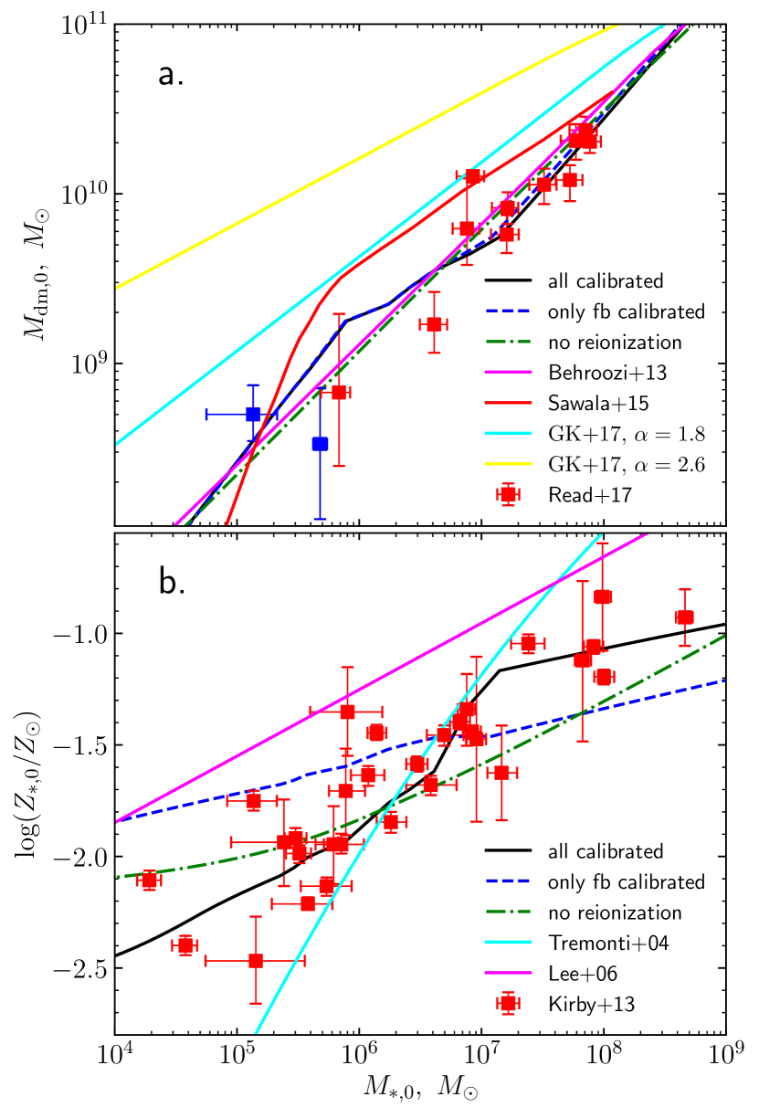
Figure 1: Relations between final stellar mass and dark matter halo mass (a) or stellar metallicity (b). Red and blue points represent data from observations (Read et al., 2017a; Kirby et al., 2013, in the top and bottom panels, respectively). Blue points denote non-isolated galaxies Carina and Leo T. Black line denotes the model with all four free parameters calibrated. Blue dashed line denotes the model with only $k_{\rm sn}$ and $\gamma_{\rm sn}$ calibrated. Green dash-dotted line denotes the model in which reionization is turned off and all 4 parameters recalibrated. In the top panel, magenta line shows the relation derived in Behroozi et al. (2013), the red line a similar relation from (Sawala et al., 2015) and the cyan and yellow lines show relations from Garrison-Kimmel et al. (2017). In the bottom panel, the cyan line is from Tremonti et al. (2004) and the magenta line is from Lee et al. (2006). See text for more details.

Our model has four free parameters: $k_{\rm sn}$ and $\gamma_{\rm sn}$ describe the efficiency of mass ejection due to stellar feedback (equation 11), $v_{\rm ej}$ is the characteristic maximal circular velocity below which galaxies lose the majority of newly-formed metals (equation 13) and $Z_{\rm igm,0}$ is the present-day IGM metallicity (equation 14). To determine the realistic values of these parameters we fit the relations between dark matter halo mass, mass-averaged stellar metallicity and stellar mass from the model to the ones from observations.

The results are presented in fig. 1. Red and blue points represent observational data (Read et al., 2017a; Kirby et al., 2013, respectively in the top and bottom panels). Blue points denote non-isolated galaxies Carina and Leo T. We fit the model parameters using orthogonal distance regression. The black line denotes a model when all four parameters were calibrated. The blue line denotes a model when only $k_{\rm sn}$ and $\gamma_{\rm sn}$ are calibrated; we set the ejected metal fraction $f_{\rm ej}=0$ (eq. 13) and $Z_{\rm igm,0}=Z_{\rm prim}$. The green line denotes a model in which the quenching of gas accretion and photoevaporation due to reionization were turned off and all four parameters were recalibrated. The relation between stellar and dark matter masses depends very weakly on $Z_{\rm igm,0}$ and $v_{\rm ej}$, as can be seen by comparing black and blue lines in fig. 1, panel a. Because of this the stellar feedback parameters $k_{\rm sn}$ and $\gamma_{\rm sn}$ can be fitted independently from $Z_{\rm igm,0}$ and $v_{\rm ej}$ by using only the relation between stellar and dark matter masses. After that, we fit $Z_{\rm igm,0}$ and $v_{\rm ej}$ by using only the stellar mass-metallicity relation. The determined parameter values are shown in table 1. We also visually analyzed the grid of parameters (intervals are shown in table 1) and found that there are no degeneracies between parameter values and the determined extremes are global.

For reference, we overplot equivalent relations from the literature in the two panels of Figure 1. In the top panel, the magenta line shows the low-mass extension of the relation $M_{*}\propto M_{\rm h}^{1.4}$ from Behroozi et al. (2013). This relation almost perfectly coincides with our result for the no-reionization case and is consistent with our other models, as expected. Similarly, the relation derived by Sawala et al. (2015, ; red line) is marginally consistent with the data and with our models. On the other hand, the two relations presented in Garrison-Kimmel et al. (2017) - cyan line for $M_{*}\propto M_{\rm h}^{1.8}$ and yellow line for $M_{*}\propto M_{\rm h}^{2.6}$ - both lie significantly above our models and the observational data, i.e. they predict much lower stellar masses at a given halo mass. This difference is also expected, since Garrison-Kimmel et al. (2017) investigated satellite galaxies in the Local Group, which are presumably significantly affected by tidal stripping and other environmental quenching effects (Geha et al., 2012; Grossi, 2019). In the bottom panel, the cyan line shows the relation derived in Tremonti et al. (2004) for a large sample of star-forming galaxies, while the magenta line shows the relation from Lee et al. (2006), derived for a small sample of nearby dwarf irregulars. Both of these relations differ significantly from our results and are much poorer matches to the observational data.

Table 1: The values of calibrated free parameters together with their grid intervals used and equation numbers in which they appear.

Parameter	Fitted value	Interval tested	Equation
$k_{\rm sn}$	0.024	[0, 1]	(11)
$\gamma_{\rm sn}$	1.47	[-3, 2]	(11)
$v_{\rm ej}$	29 km/s	[10, 100] km/s	(13)
$Z_{\rm igm,0}$	0.0023	[$2\cdot 10^{-5}$, 0.01]	(14)

Figure 2 shows the relations between gas mass, gas metallicity, SFR and stellar mass at $z=0$. Once again, points are observational data, from Oh et al. (2015); Kirby et al. (2017); Berg et al. (2012); McGaugh et al. (2017) and the lines represent our model results with different calibrations, as in Figure 1. These three relations were not used for parameter calibration and they are not simple consequences of the two relations used for calibration. Therefore, the good match between observations and the fully calibrated model (black lines) in all these relations strongly suggests that our model captures the salient features of isolated dwarf galaxy evolution. Some discrepancy between the best-fit model and observed gas metallicities most likely arises due to our over-simplified treatment of enrichment, echoing the results of earlier semi-analytic models (Starkenburg et al., 2013). Clear discrepancies between the model with reionization turned off and the observations seen in panels a and b show that the modeling of the effects of reionization is necessary in order to simultaneously reconstruct all of the observed relations.

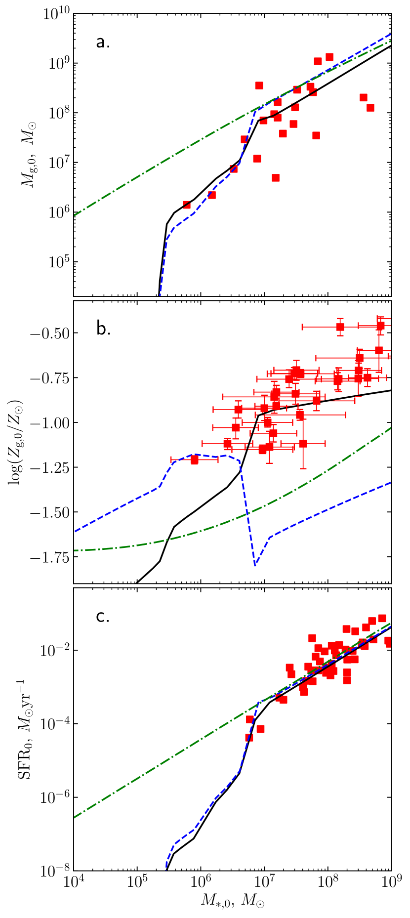
Figure 2: Relations between stellar mass and gas mass (a), gas metallicity (b), SFR (c) at $z=0$. Red points represent data from observations (Oh et al., 2015; Kirby et al., 2017; Berg et al., 2012; McGaugh et al., 2017). Lines denote the same models as in fig 1.

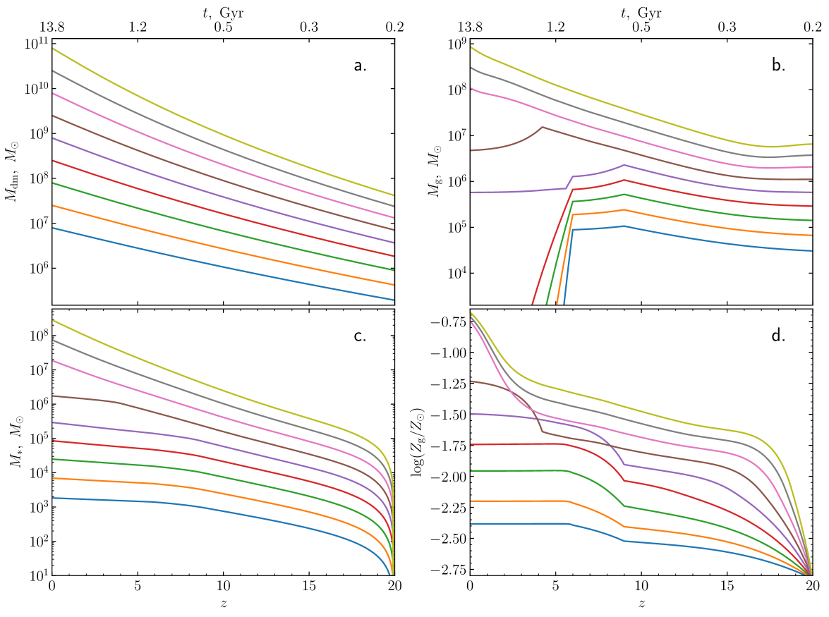
Figure 3: Dependence of the dark matter halo mass, the gas mass, the stellar mass and the gas metallicity on redshift in the average model. Different colored lines denote models with different final dark matter halo masses.

All of the calibrated parameters have a clear physical interpretation and therefore it is useful to discuss the implications of their values. The values of $k_{\rm sn}$ and $\gamma_{\rm sn}$ determine the fraction of supernova energy that is used to eject gas from a galaxy. The amount of ejected gas per supernova scales as $m_{\rm ej}\propto v_{\rm max}^{\gamma_{\rm sn}-2}$ (cf eq. 10). Therefore, since $\gamma_{\rm sn}<2$, the mass ejected per supernova explosion decreases with increasing galaxy mass, as may be expeceted due to the increasing gravitational potential. However, the efficiency of ejection increases, since $\gamma_{\rm sn}>0$. This might be explained by the fact that in a larger galaxy there is a higher chance for radiated supernova energy to be reabsorbed again and so on average a higher fraction of supernova energy might be used to heat the gas. The normalization of the efficiency, $k_{\rm sn}=2.4\%$, is similar to the analytically-derived $k\sim 3\%$ of the supernova energy injected as kinetic energy into interstellar turbulence (Spitzer, 1990).

The present-day metallicity of the IGM is not known with certainty because of difficulties in measuring it, but our calibrated value is not implausible according to both observational and theoretical estimates (Cen & Chisari, 2011). The calibrated value of $v_{\rm ej}$ also seems realistic because galaxies with lower maximal circular velocities have virial temperatures close to or lower than $10^{4}$ K which is a typical temperature of ionized interstellar gas. Because the newly-formed metals are typically ejected into the environments ionized due to stellar feedback, it seems plausible that a major fraction of them are lost in galaxies with virial temperatures lower than $10^{4}$ K.

4 Evolution of observable parameters

4.1 Evolution of average models

Having determined the values of the free parameters that give the best results for modern-day dwarf galaxies, we now turn to the evolution of model galaxy parameters over cosmic time. Figure 3 shows how the dark matter halo mass, the gas mass, the stellar mass and the gas metallicity depend on redshift in the average model. The nine lines in each panel correspond to models with different present-day halo masses, from $8\times 10^{6}\,{\rm M_{\odot}}$ to $8\times 10^{10}\,{\rm M_{\odot}}$ in steps of $0.5$ dex.

The mass of the dark matter halo (Figure 3, panel a) grows smoothly in all models because the effect of galaxy mergers is smoothed over time and we model only isolated galaxies that do not experience significant perturbations to their halos.

Evolution of the gas mass (panel b of Figure 3) shows several sudden breaks for galaxies with final halo masses below $5\times 10^{9}\,{\rm M_{\odot}}$ (fourth line from the top and lower). The earliest break, at $z\approx 9$, occurs due to the start of the reionization epoch. In the five lowest-mass models, smooth gas accretion turns off (see section 2.4) and those galaxies can then increase their gas masses only via mergers, at least until their virial temperature grows above the threshold value. We tested that our results are mostly insensitive to the precise redshift of the start of reionization, by varying that parameter in the range $6<z_{\rm reion}<15$. Reionization ends at $z=6$; this results in a second break in gas mass, because from then on, galaxies with low enough virial temperatures begin losing gas due to evaporation. Evaporation can cease only if the virial temperature in the galaxy grows large enough. This happens in the model with final halo mass $8\times 10^{8}\,{\rm M_{\odot}}$ (violet line, fifth from the top) at $z\simeq 5.5$, resulting in another sudden break in gas mass evolution. Conversely, in a slightly more massive galaxy (brown line, fourth from the top), virial temperature grows more slowly than $T_{\rm eq}\left(\Delta_{\rm vir}/3\right)$, eventually stopping the smooth accretion of IGM gas at $z\simeq 4$, producing another break. Even in the three most massive galaxies, where the virial temperature always remains higher than $T_{\rm eq}\left(\Delta_{\rm vir}/3\right)$, there are small effects on gas mass due to reionization. They occur because a fraction of the infalling gas comes from mergers with smaller galaxies which are strongly affected by reionization.

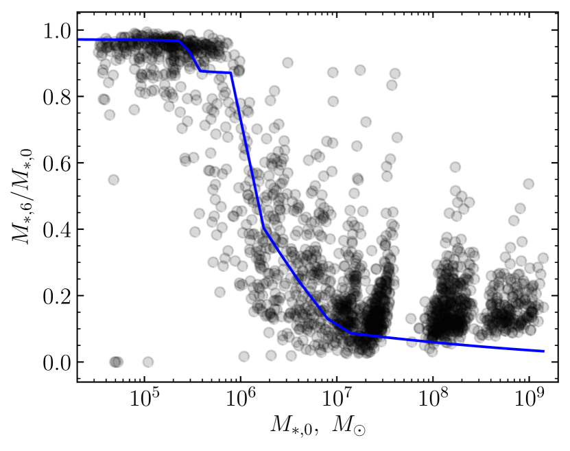
Figure 4: Fraction of stars formed before $z=6$ as a function of present-day stellar mass in average (blue line) and stochastic models (grey circles).

SFR in our model is directly proportional to gas mass, therefore the total stellar mass (Fig 3, panel c) shows similar evolutionary stages as the gas mass. Additionally, stellar mass may grow in fully quenched galaxies due to mergers. Since we do not deal with processes during which the stellar mass could decrease, e.g. tidal stripping, stellar mass grows even in the least massive galaxies. It is clear that stars with low present-day halo and stellar masses form most of their stellar mass at high redshift; in fact, galaxies with $M_{*,0}\leq 3\times 10^{5}\,{\rm M_{\odot}}$ (five lowest-mass models) have more than half their present-day stellar mass in place by $z=6$; we show below that the mass increase since then is actually only due to mergers, rather than in-situ star formation. The most massive galaxies, conversely, form the majority of their stars after reionization.

The computed star formation histories can be compared with observations of dwarf galaxies in the Local Group (Weisz et al., 2014a). While they exhibit a wide variety of star formation histories, a general trend of smaller galaxies forming most of their stars at earlier epochs is evident. In particular, galaxies with present-day stellar mass $M_{*,0}\leq 10^{5}\,{\rm M_{\odot}}$ have, on average, formed $f_{6}\sim 80\%$ of their stars by $z=6$, although the spread in this fraction is large, $25\%<f_{6}<90\%$ (see Figure 10 of Weisz et al., 2014a). In galaxies with $10^{5}\,{\rm M_{\odot}}<M_{*,0}\leq 10^{6}\,{\rm M_{\odot}}$, the average fraction drops to $f_{6}\sim 40\%$. We show our model results in Figure 4, in blue line for average models and grey circles for stochastic models (see Section 4.2 below). The smallest model galaxies, with $M_{*,0}\lower 2.15277pt\hbox{$\;\buildrel<\over{\sim}\;$}4\times 10^{5}\,{\rm M_{\odot}}$, have $f_{6}\simeq 90-100\%$, with the rest of their stellar mass built up only through mergers. In more massive galaxies, this fraction drops: in galaxies with $M_{*,0}>10^{7}\,{\rm M_{\odot}}$, we find $f_{6}\leq 10\%$. It is important to note, however, that this fraction only accounts for star formation in the main branch of the merger tree that eventually forms the present-day galaxy. Since the largest galaxies are merging with many smaller haloes that have $f_{6}>10\%$, the actual fraction of stars in the present-day galaxy with formation times later than $z=6$ would be larger than $10\%$. This becomes evident when analysing the star formation histories of the stochastic models (Section 4.2). The rapid transition between quenched and non-quenched populations at $M_{*,0}\simeq 2\times 10^{6}\,{\rm M_{\odot}}$ suggests that there should be a clear break in mass-weighted ages of the stellar populations of dwarf galaxies with different stellar masses.

The gas metallicity evolution shown in Figure 3, panel d, can be understood qualitatively from gas and stellar mass evolution. In the smallest galaxies, star formation continues for a while after the shut-off of smooth gas accretion, enriching the ISM rapidly because it is not diluted by the infalling low-metallicity IGM gas. Once the remaining gas is depleted, mainly by evaporation, star formation ceases and gas metallicity remains constant until the present day. In the most massive galaxies metallicity starts to increase faster at $z<3$ because of enrichment of the IGM material accreting on to those galaxies, in addition to in-situ enrichment by stars. It is worth noting that once smooth gas accretion shuts off in a galaxy, its gas metallicity may increase rapidly to values larger than those in a more massive galaxy that is still accreting gas from the IGM (exemplified by the crossing of the violet, brown and pink lines, the fourth, fifth and sixth most massive galaxy models, at intermediate redshifts). Therefore high-redshift dwarf galaxy populations may show an inverted slope in some part of their mass-metallicity relation.

4.2 Star formation in stochastic models

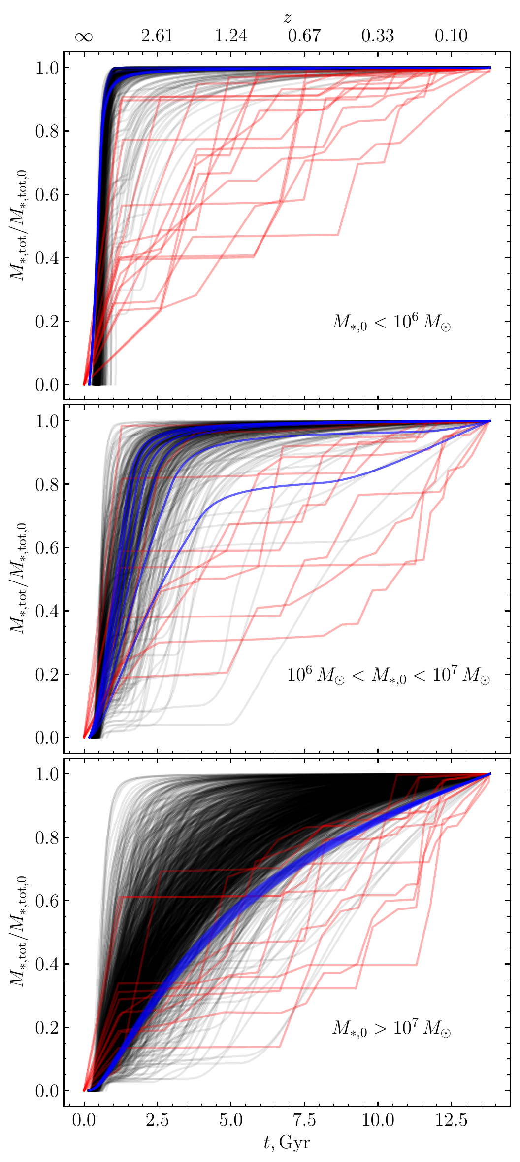
Figure 5: Cumulative star formation histories of model galaxies (grey lines for stochastic models, blue lines for average models) compared with observationally-derived SFHs from Weisz et al. (2014a, red lines). Each panel shows a different present-day stellar mass bin, as indicated.

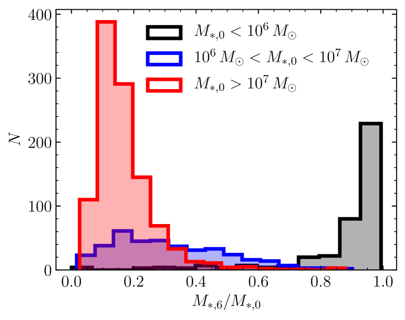
Figure 6: Fractional star formation before $z=6$ in stochastic models of galaxies with different present-day stellar masses: $M_{\rm*,0}<10^{6}\,{\rm M_{\odot}}$ (black), $10^{6}\,{\rm M_{\odot}}<M_{\rm*,0}<10^{7}\,{\rm M_{\odot}}$ (blue) and $M_{\rm*,0}>10^{7}\,{\rm M_{\odot}}$ (red).

The stochastic models and their star formation histories provide a picture of how reionization affects galaxies with different mass assembly histories. Grey circles in figure 4 show the fraction $f_{6}$ of stars formed before $z=6$ in the stochastic models, while figure 5 shows the cumulative star formation histories of our stochastic model galaxies (grey lines), average model galaxies (blue lines) and observed Local Group galaxies from (Weisz et al., 2014a, red lines). Following Weisz et al. (2014a), we separate the galaxies into three bins by present-day stellar mass.

Two things are immediately clear from these plots. First of all, stochasticity of mass assembly has a significant effect on the star formation histories. In small galaxies ($M_{*,0}<10^{6}\,{\rm M_{\odot}}$), stochastic assembly means that some galaxies are more resilient to reionisation and therefore can form a significant fraction of their stars after $z=6$. In massive galaxies ($M_{*,0}>10^{7}\,{\rm M_{\odot}}$), conversely, stochasticity leads to, on average, older stellar populations than the average model, because some of these galaxies are significantly quenched just after reionisation and because the stochastic models account for dry mergers with small galaxies containing only very old stars (see penultimate paragraph of Section 4). For intermediate-mass galaxies ($10^{6}\,{\rm M_{\odot}}<M_{*,0}<10^{7}\,{\rm M_{\odot}}$), stochasticity mainly increases the spread of possible SFHs without changing the mean values.

The second observation to make is that observed galaxies generally have younger stellar populations than model galaxies, both average and stochastic ones. This discrepancy is particularly pronounced for the smallest galaxies: even though stochastic models produce a spread of the fraction of stars formed before reionisation, with a few outlier galaxies forming the majority of their stars after $z=6$, the observed SFHs with very late star formation are not reproduced. Most of our smallest galaxies are completely quenched by reionisation, in marked contrast to observations (Weisz et al., 2014b). Similarly, our models produce more than $60\%$ of stars by $t=2$ Gyr in galaxies with $M_{*,0}<10^{6}\,{\rm M_{\odot}}$, but very few observed ones do so. The differences are somewhat smaller in more massive galaxies.

There may be a few causes of this discrepancy. First of all, our models do not include any environmental effects. Collisions with intergalactic gas streams may reignite star formation in even the smallest galaxies (Wright et al., 2019). In fact, spheroidal galaxies show on average earlier star formation than irregulars (Weisz et al., 2014a), suggesting that interactions likely played a significant role in prolonging and/or reigniting their star formation. Another effect is starbursts caused by gas compression during major mergers, which we neglect (see Section 2.8). Overall, mergers lead to bursts or even prolonged periods of star formation (Cloet-Osselaer et al., 2014; Fouquet et al., 2017), so this effect may be important to some extent. On the other hand, the overall importance of mergers to the SFHs of dwarf galaxies has been recently questioned (Fitts et al., 2018), so it is difficult to determine the magnitude of this effect. Finally, we assume complete homogeneity of the Universe, and that reionization happens simultaneously everywhere. In reality, the growth of HII bubbles was very patchy (Furlanetto et al., 2004; Furlanetto & Oh, 2005; Holder et al., 2007). The effect of patchy growth is cumulative with that of gas accretion and mergers: in denser regions, reionization occurs later, gas accretion is faster and mergers more frequent. All three effects can lead to some galaxies continuing to form stars until much later times, as seen in detailed numerical simulations (Katz et al., 2019).

The trend of star formation histories changing with increasing mass is qualitatively preserved in our models: in small galaxies, most stars are formed early, while massive galaxies have prolonged SFHs, with the switchover happening at present-day halo masses $2\times 10^{9}\,{\rm M_{\odot}}\lower 2.15277pt\hbox{$\;\buildrel<\over{\sim}\;$}M_{\rm dm,0}\lower 2.15277pt\hbox{$\;\buildrel<\over{\sim}\;$}6\times 10^{9}\,{\rm M_{\odot}}$, corresponding to stellar masses $10^{6}\,{\rm M_{\odot}}\lower 2.15277pt\hbox{$\;\buildrel<\over{\sim}\;$}M_{\rm*,0}\lower 2.15277pt\hbox{$\;\buildrel<\over{\sim}\;$}10^{7}\,{\rm M_{\odot}}$. We show this in Figure 6, where the three histograms present the spread of fractions of stars formed before reionization in stochastic models of galaxies falling in the three mass bins described above. It is clear that there is a transition between early and late star formation modes in this mass range, with the vast majority of $M_{\rm*,0}<10^{6}\,{\rm M_{\odot}}$ galaxies forming $>80\%$ of their stars before $z=6$, while for galaxies with $M_{\rm*,0}>10^{7}\,{\rm M_{\odot}}$, the majority form $<40\%$ of stars at such early. Galaxies with intermediate stellar masses represent a transitioning population, with models exhibiting both significant late star formation and almost complete quenching by reionization.

4.3 Build-up of observed correlations

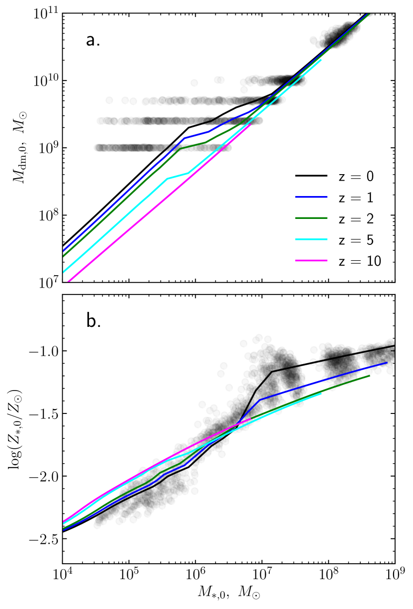
Figure 7: Same relations as in fig. 1 but now differently colored lines denote the average model at different redshifts. The black points represent the tree model with various different mass-assembly histories.

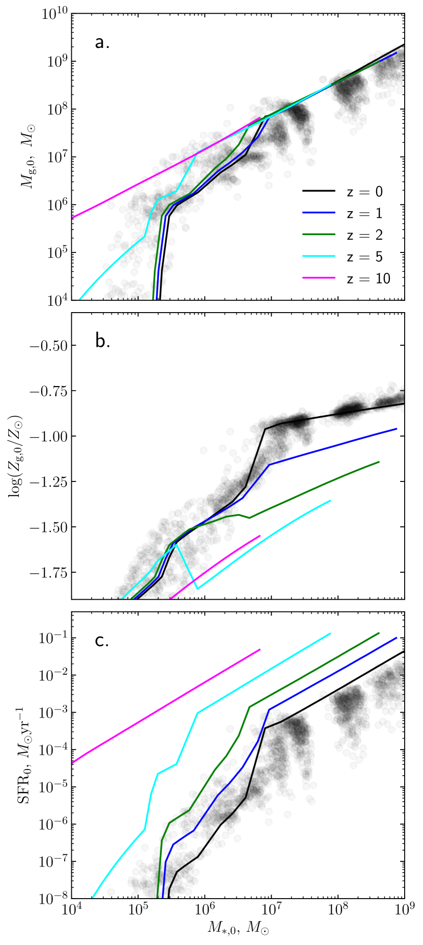
Figure 8: Same relations as in fig. 2 with same markings as in fig. 7.

We now turn to investigating the correlations between present-day dwarf galaxy parameters, the evolution of these correlations with redshift, and the spread of individual galaxy parameters around the average correlations. We use the average models to investigate relation evolution, and the properties of the 1500 stochastic models at $z=0$ to investigate individual variations.

Figures 7 and 8 show the same relations as figures 1 and 2. However, here we plot the relations at different cosmological epochs with different-coloured lines: $z=10$ in magenta, $z=5$ in cyan, $z=2$ in green, $z=1$ in blue and $z=0$ in black. In addition, semi-transparent gray circles show the properties of individual galaxies from stochastic models at $z=0$. These values can be seen as the dispersion around the average model $z=0$ line due to effects of stochasticity.

The break in the $M_{\rm dm}-M_{*}$ relation (figure 7, panel a) in the average model is evident as early as $z=5$ and persists until the present day, with the only change being the halo mass at which it occurs. The origin of the break, as discussed in subsection 4.1, is the effect of reionisation clearing gas out of the smallest galaxies, shutting off their star formation. The precise effect on each galaxy around the break mass depends sensitively on its mass assembly history, as evidenced by the stochastic models. These show not a clear break, but a significant spread of stellar masses for each final halo mass around the break. Some galaxies assemble their halo masses early on and can continue forming stars until low redshift, while others spend a significant amount of time quenched by reionisation, sometimes reigniting at late times (see Paper I). A similar spread is present at higher redshifts as well (see section 4.2 above).

All other relations show noticeable breaks at stellar masses $M_{*}\simeq 10^{7}\,{\rm M_{\odot}}$, both in the average and the stochastic models. It is worth noting, however, that those breaks appear very differently at higher redshift. For example, the $M_{*}-Z_{*}$ relationship shows a break only at $z\leq 1$, while the $M_{*}-M_{\rm g}$ and $M_{*}-$SFR relationships show a clear break as early as $z=5$, although the stellar mass at which the break occurs increases with time. The $M_{*}-Z_{\rm g}$ relationship is even more different, with an inverse break at $2\leq z\leq 5$, no break at $z=10$ and a positive break at $z\leq 1$. All of these breaks also arise due to reionization, but the timescale for them to appear is different. Gas mass and the closely related SFR decrease very rapidly in the smallest galaxies. Stellar metallicity, on the other hand, does not decrease, but merely stops increasing in those galaxies, while it continues to grow in the larger ones, as evident from figure 7, panel b, when looking at the average model curves. Gas metallicity increases rapidly in quenched galaxies, creating a negative slope, until the stars in more massive galaxies have enough time to ‘catch up’ and enrich the gas further. This variation in the evolution of observable relations suggests that high-redshift dwarf galaxies may exhibit very different correlations between parameters than local ones. In particular, differences due to reionization only manifest strongly at $z<2$, and become more pronounced with time, so local galaxies may provide better evidence of reionization effects than high-redshift ones.

The stochastic models reveal how the variation of mass assembly affects the relations. Both metallicity relations exhibit a spread around the $z=0$ value of the average model. The spread of stellar metallicities is $\pm\sim 0.25$ dex around the break mass, and smaller for both more and less massive galaxies. Gas metallicity has a large spread of $\pm\sim 0.2$ dex at low galaxy masses, but practically zero spread for galaxies above the break, which all experience rather similar growth of stellar mass, and hence enrichment of the ISM.

The gas masses in stochastic models are systematically smaller than in the average model. Correspondingly, the SFRs are lower as well. The reason for this is that stochastic models spend some time at lower halo masses than corresponding average models, as well as some time at higher masses. However, being at a lower halo mass can bring a given stochastic model under the threshold for gas evaporation, while being at a higher mass does not give a corresponding advantage to gas accretion. As a result, stochastic models tend to lose more gas to evaporation than average models. This is evident to some extent in the $M_{\rm dm}-M_{*}$ relation, where stochastic models have a bigger spread toward lower stellar masses at a given halo mass than toward higher stellar masses. This effect slightly reduces the alignment of our model results to the observational data (figure 2, panel c).

Comparing the average models at high redshift to both average and stochastic models at low redshift reveals that galaxies at high redshift were significantly different from modern-day ones, especially in their gas properties and SFRs. This evolution of gas mass, gas metallicity and SFR at a given $M_{*}$ or $M_{\rm dm}$ occurs even though these galaxies are all isolated. The extreme evolution in SFRs (SFR decreases by almost four orders of magnitude from $z=10$ for galaxies with $M_{*}=10^{6}\,{\rm M_{\odot}}$ and two orders of magnitude for $M_{*}=10^{7}\,{\rm M_{\odot}}$) occurs both because of gas depletion and because of passive evolution of galaxy sizes: modern galaxies are less compact, therefore have lower gas surface densities and lower molecular gas fractions, which lead to lower SFRs even for identical gas masses.

5 Discussion

5.1 Trends of dwarf galaxy properties

Qualitatively, the evolution of the $M_{*}-$ SFR relation that we find in our models agrees with the observed evolution (Tasca et al., 2015; Santini et al., 2017), although the latter is derived for more massive galaxies. In particular, the specific SFR (SFR$/M_{*}$) increases with redshift, and galaxies have similar specific SFRs across the mass range at a given redshift. Quantitatively, the specific SFR in the most massive galaxies in our models is lower by a factor of a few than the average observational result, both at $z=0$ (Peng et al., 2010) and at higher redshift (Tasca et al., 2015; Santini et al., 2017). The SFRs observed in low-mass galaxies agree very closely with our model results, however (figure 2, panel c). The reason for this is that our models are calibrated using data of isolated dwarf galaxies, which comprise only a small fraction of typically observed galaxies. They tend to have lower SFRs than average, since they are not affected by their environment, which may cause shocks and lead to starbursts.

The predicted trend of the mass-metallicity relation, if extended to higher stellar masses, would also give slightly lower metallicities than observed ($Z\simeq Z_{\odot}$ at $M_{*}=10^{9}\,{\rm M_{\odot}}$, cf. Sánchez et al., 2017). It should be noted, however, that metallicities decrease steeply at $M_{*}<10^{9}\,{\rm M_{\odot}}$, and the data available for these smaller galaxies generally agrees with our results (figure 1, panel b). Matching the trend obtained in our models to that observed for more massive galaxies is not possible without a more detailed treatment of enrichment of the ISM, the escape of metals into the IGM, and effects such as the galactic fountain.

The $M_{*}-M_{\rm g}$ relation agrees very well with that observed in small galaxies, but observations show a break at $M_{*}\simeq 10^{9}-10^{10}\,{\rm M_{\odot}}$, with more massive galaxies having a shallower slope (Lelli et al., 2016; McGaugh et al., 2017). Therefore we expect that our model would overpredict the gas masses of more massive galaxies. This is expected, since AGN outflows, which are not included in our model, should become significant to galaxy evolution at masses $M_{*}\lower 2.15277pt\hbox{$\;\buildrel>\over{\sim}\;$}10^{10}\,{\rm M_{\odot}}$ (Martín-Navarro & Mezcua, 2018; Zubovas, 2018).

5.2 Stochasticity of dwarf galaxy evolution

There is a large volume of work exploring the importance to dwarf galaxy evolution of various stochastic effects, such as star formation (Gerola et al., 1980; Matteucci & Chiosi, 1983; Orban et al., 2008; Weisz et al., 2008; Mineikis & Vansevičius, 2010; Weisz et al., 2012; Applebaum et al., 2020), reionization (Bose et al., 2018; Katz et al., 2019), mergers (Laporte & Penarrubia, 2015; Benítez-Llambay et al., 2015; Macciò et al., 2017; Anglés-Alcázar et al., 2017) or other environmental interactions (Peñarrubia et al., 2012). In addition, stochastic processes may affect the appearance and inferred properties of dwarf galaxies, e.g. their star formation rates (da Silva et al., 2014), H$\alpha$ luminosities (Fumagalli et al., 2011) or their contribution to reionization (Forero-Romero & Dijkstra, 2013). Our work contributes to this field by looking at stochasticity from another angle: the differences in halo assembly histories of individual galaxies, which is related to, but somewhat broader in scope than, the stochasticity of merger events.

The differences between properties of galaxies in average and stochastic models show that stochasticity of mass assembly is an important element of dwarf galaxy evolution, in general agreement with semi-analytical models based on N-body simulation results (Yaryura et al., 2016). Stochasticity induces a spread in the observable relations around the mean value. Additionally, for galaxies with $M_{*}>10^{7}\,{\rm M_{\odot}}$, our stochastic models predict significantly lower gas masses and SFRs for a given value of $M_{*}$ than average models; for galaxies with $M_{*}<10^{7}\,{\rm M_{\odot}}$, stochastic models predict higher average halo masses and somewhat higher gas masses and SFRs.

The main reason for these systematic differences is the different responses of halos to reionization. The more massive a given halo is at $z=6$, the less it is affected by reionization, the more gas it retains and the more stars it can form. Halos with present-day masses $M_{\rm dm,0}>10^{10}\,{\rm M_{\odot}}$, typically hosting galaxies with $M_{*,0}>10^{7}\,{\rm M_{\odot}}$, have large enough masses at $z=6$ in the average model that they are affected very little by reionization. Halos in stochastic models have both larger and smaller masses than those in the average model, but those with higher masses evolve very similarly to the average ones; conversely, those with lower masses are affected more significantly by reionization. Later on, these halos merge with smaller galaxies that retain much less gas, leading to lower gas masses and SFRs at lower redshift. For smaller halos, variations of mass assembly history become more significant. Halos that build up their mass early are less affected by reionization, retain their gas and form stars efficiently, generally following the trends in $M_{*}-M_{\rm dm}$ and other relations set by larger galaxies. However, halos that assemble later are strongly affected, leading to earlier truncation of star formation and lower present-day stellar mass. Some of these galaxies can be re-ignited at later times if mergers bring their masses above the evaporation threshold (see Paper I), therefore a fraction of these galaxies have higher gas masses and SFRs than predicted by the average model.

The spread in halo mass, gas mass, stellar and gas metallicity, and star formation rate at a given stellar mass in our stochastic models (Figures 7 and 8) is similar to that in real galaxies Read et al. (Figures 1 and 2; also see 2017b); Kirby et al. (Figures 1 and 2; also see 2013); Oh et al. (Figures 1 and 2; also see 2015); Kirby et al. (Figures 1 and 2; also see 2017); Berg et al. (Figures 1 and 2; also see 2012); McGaugh et al. (Figures 1 and 2; also see 2017). It appears that stochastic differences of halo mass assembly can account for most of the spread of observed gas masses and star formation rates in modern-day dwarf galaxies without invoking any other physical processes.

We deliberately chose to include only this aspect of stochasticity while neglecting other potential sources. In particular, we fixed the redshift of the end of reionization for all simulations, the star formation prescription is purely deterministic and there are no environmental interactions included. Taken together, these sources of stochasticity may account for the whole spread of dwarf galaxy properties. It would be interesting to see how these processes interact with each other and what their relative contributions to total variation of dwarf galaxy parameters are, but such an investigation is beyond the scope of this paper. Nevertheless, our simulations show that stochasticity of mass assembly should be kept in mind when interpreting observed dwarf galaxy properties and following their evolution with semi-analytic models.

Acknowledging and understanding the importance of stochasticity will also help make better predictions regarding observable dwarf galaxy trends. Some of the parameters in the stochastic models, e.g. gas and stellar metallicity, follow the average models quite closely, while others, e.g. gas mass and SFR, are spread out rather widely. The latter parameters are therefore poor choices when trying to constrain the position of the break in dwarf galaxy properties at $M_{*}\sim 10^{7}\,{\rm M_{\odot}}$, since identification of the break would require a large number of data points with small errors. The mass at which the break occurs depends on the process of reionization (Bose et al., 2018; Katz et al., 2019) and can help us infer its properties, therefore it is important to know whether the observed breaks are due to individual stochastic variations or global trends.

5.3 Starbursts and star formation quenching

Our stochastic models do not show any starburst dwarf galaxies with specific star formation rates SFR$/M_{*}>1$ Gyr^-1. To some extent, this is an artifact of our model, where we do not account for possible shocks during galaxy mergers increasing the efficiency of star formation, not do we account for the triggering of star formation by supernovae or AGN effects. The observed starburst fraction does not depend strongly on galaxy mass (Bergvall et al., 2016), so we may expect a few percent of dwarf galaxies to also be in starburst mode at the present time. The overall influence of starbursts on integrated galaxy properties appears to be small (Bergvall et al., 2016), therefore the lack of starbursts in our model should not affect the overall results very much.

Some of the galaxies in the stochastic models have very low gas masses and, as an extention, very low SFRs. Their specific SFRs can fall as low as $10^{-3}$ Gyr^-1. Such galaxies may correspond to the observed dwarf spheroidal (dSph) galaxies, which are generally quenched. The quenching in our models is, however, not a consequence of a starburst or some other internal process, but rather of the mass assembly history preventing gas accretion on to them for significant periods of time. Virtually all galaxies with $M_{*}<10^{7}\,{\rm M_{\odot}}$ fall into this group and a small fraction of more massive ones also do. As more observational data is collected, population analysis of dwarf galaxy specific star formation rates may provide insight into the importance of internal versus external quenching processes. If dSph and other types of quenched dwarf galaxies form a significant fraction of $M_{*}>10^{7}\,{\rm M_{\odot}}$ galaxies at $z=0$, it would mean that starbursts and other internal processes are important quenching channels, since the population would not be explained purely by different mass assembly histories and the effect of the ionizing background radiation. In the future, we plan to extend our model to include better treatment of starbursts, AGN feedback and galaxy-galaxy interactions to account for these effects.

5.4 Galaxy properties at very low stellar masses

Observational data of dwarf galaxies below $M_{*}\sim 10^{7}\,{\rm M_{\odot}}$ is scarce (e.g., Berg et al., 2012; Oh et al., 2015; Kirby et al., 2017; Read et al., 2017a; McGaugh et al., 2017), therefore checking the existence of the break predicted by our model is difficult. The few data points at lower stellar masses generally seem to agree with our results, but it will be very interesting to get more information about these smallest dwarf galaxies. Observations of high-redshift galaxies and their properties also have only limited overlap with the mass range of dwarf galaxies (e.g., Santini et al., 2017). Therefore it will be very important to test the model with larger data sets extending down to lower masses and higher redshift, such as could be provided by the upcoming Euclid space observatory (Laureijs et al., 2011). Most importantly, they will help better understand the transition region between dwarf galaxies, dominated by stellar feedback, and AGN-dominated massive galaxies. In addition, our model should help better understand the relative importance of internal (e.g. supernova feedback) and external (e.g. intergalactic radiation field) processes to dwarf galaxy evolution.

The relationship between gas metallicity and stellar mass is particularly interesting and may be the most illuminating when it comes to high-redshift galaxy properties. The reversal of its trend, with metallicity decreasing with increasing stellar mass, over a certain mass range for a range of redshifts, should help us better understand the enrichment of the ISM and IGM by stellar processes (see sections 2.6 and 2.7).

6 Conclusions

In this paper, we presented results of a semi-analytical model following the evolution of isolated dwarf galaxies from early Universe until the present day. Our model uses a few free parameters, but when they are calibrated using the halo mass - stellar mass and stellar mass-metallicity relations, the model fits other observed properties of the local dwarf galaxy population remarkably well. The relations are generally affected very strongly by reionization, which suppresses gas infall in the smallest galaxies, even evaporating some of them. Different relations acquire their characteristic shapes at different times. At the present day, most of them exhibit a break at $M_{*}=10^{7}\,{\rm M_{\odot}}$, with smaller galaxies being significantly affected by reionization, and larger ones being affected only indirectly, by changes to the small galaxies that merged with them over the Hubble time. The position of the break depends on the properties of reionization, so in principle could be used to test these properties, once larger samples of isolated dwarf galaxy properties become available.

We also find that the stochasticity of mass assembly histories has a strong effect on dwarf galaxy gas masses and SFRs. Models not accounting for this effect may overpredict the gas mass and SFR for a galaxy with a given dark matter halo and stellar mass, leading to incorrect determination of dwarf galaxy properties or incorrect calibration of model parameters.

Our results suggest that future observations, that will reveal large samples of low-mass high-redshift galaxies, will be instrumental in understanding the evolution of these galaxy building blocks.

References

- Anglés-Alcázar et al. (2017) Anglés-Alcázar D., Faucher-Giguère C.-A., Kereš D., Hopkins P. F., Quataert E., Murray N., 2017, MNRAS, 470, 4698
- Applebaum et al. (2020) Applebaum E., Brooks A. M., Quinn T. R., Christensen C. R., 2020, MNRAS, 492, 8
- Asplund et al. (2009) Asplund M., Grevesse N., Sauval A. J., Scott P., 2009, ARA&A, 47, 481
- Barkana & Loeb (1999) Barkana R., Loeb A., 1999, ApJ, 523, 54
- Baugh (2006) Baugh C. M., 2006, Reports on Progress in Physics, 69, 3101
- Behroozi et al. (2013) Behroozi P. S., Wechsler R. H., Conroy C., 2013, ApJ, 770, 57
- Benítez-Llambay et al. (2015) Benítez-Llambay A., Navarro J. F., Abadi M. G., Gottlöber S., Yepes G., Hoffman Y., Steinmetz M., 2015, MNRAS, 450, 4207
- Berg et al. (2012) Berg D. A., et al., 2012, ApJ, 754, 98
- Bergvall et al. (2016) Bergvall N., Marquart T., Way M. J., Blomqvist A., Holst E., Östlin G., Zackrisson E., 2016, A&A, 587, A72
- Bermejo-Climent et al. (2018) Bermejo-Climent J. R., et al., 2018, MNRAS, 479, 1514
- Blanc et al. (2019) Blanc G. A., Lu Y., Benson A., Katsianis A., Barraza M., 2019, ApJ, 877, 6
- Bose et al. (2018) Bose S., Deason A. J., Frenk C. S., 2018, ApJ, 863, 123
- Brooks et al. (2013) Brooks A. M., Kuhlen M., Zolotov A., Hooper D., 2013, ApJ, 765, 22
- Bryan & Norman (1998) Bryan G. L., Norman M. L., 1998, ApJ, 495, 80
- Carlin et al. (2016) Carlin J. L., et al., 2016, ApJ, 828, L5
- Cen & Chisari (2011) Cen R., Chisari N. E., 2011, ApJ, 731, 11
- Cloet-Osselaer et al. (2014) Cloet-Osselaer A., De Rijcke S., Vandenbroucke B., Schroyen J., Koleva M., Verbeke R., 2014, MNRAS, 442, 2909
- Dawoodbhoy et al. (2018) Dawoodbhoy T., et al., 2018, MNRAS, 480, 1740
- Dijkstra et al. (2004) Dijkstra M., Haiman Z., Rees M. J., Weinberg D. H., 2004, ApJ, 601, 666
- Drlica-Wagner et al. (2015) Drlica-Wagner A., et al., 2015, ApJ, 813, 109
- Efstathiou (1992) Efstathiou G., 1992, MNRAS, 256, 43P
- Efstathiou (2000) Efstathiou G., 2000, MNRAS, 317, 697
- Elbaz et al. (2011) Elbaz D., et al., 2011, A&A, 533, A119
- Fakhouri et al. (2010) Fakhouri O., Ma C.-P., Boylan-Kolchin M., 2010, MNRAS, 406, 2267
- Finlator & Davé (2008) Finlator K., Davé R., 2008, MNRAS, 385, 2181
- Fitts et al. (2018) Fitts A., et al., 2018, MNRAS, 479, 319
- Forero-Romero & Dijkstra (2013) Forero-Romero J. E., Dijkstra M., 2013, MNRAS, 428, 2163
- Fouquet et al. (2017) Fouquet S., Łokas E. L., del Pino A., Ebrová I., 2017, MNRAS, 464, 2717
- Fryer et al. (2012) Fryer C. L., Belczynski K., Wiktorowicz G., Dominik M., Kalogera V., Holz D. E., 2012, ApJ, 749, 91
- Fumagalli et al. (2011) Fumagalli M., da Silva R. L., Krumholz M. R., 2011, ApJ, 741, L26
- Furlanetto & Oh (2005) Furlanetto S. R., Oh S. P., 2005, MNRAS, 363, 1031
- Furlanetto et al. (2004) Furlanetto S. R., Zaldarriaga M., Hernquist L., 2004, ApJ, 613, 1
- Garrison-Kimmel et al. (2017) Garrison-Kimmel S., Bullock J. S., Boylan-Kolchin M., Bardwell E., 2017, MNRAS, 464, 3108
- Garrison-Kimmel et al. (2019) Garrison-Kimmel S., et al., 2019, MNRAS, 489, 4574
- Geha et al. (2012) Geha M., Blanton M. R., Yan R., Tinker J. L., 2012, ApJ, 757, 85
- Genel et al. (2010) Genel S., Bouché N., Naab T., Sternberg A., Genzel R., 2010, ApJ, 719, 229
- Gerola et al. (1980) Gerola H., Seiden P. E., Schulman L. S., 1980, ApJ, 242, 517
- Gnedin (2000) Gnedin N. Y., 2000, ApJ, 542, 535
- Grossi (2019) Grossi M., 2019, in McQuinn K. B. W., Stierwalt S., eds, IAU Symposium Vol. 344, Dwarf Galaxies: From the Deep Universe to the Present. pp 319–330 (arXiv:1811.03647), doi:10.1017/S1743921318007159
- Heger et al. (2003) Heger A., Fryer C. L., Woosley S. E., Langer N., Hartmann D. H., 2003, ApJ, 591, 288
- Hoeft et al. (2006) Hoeft M., Yepes G., Gottlöber S., Springel V., 2006, MNRAS, 371, 401
- Holder et al. (2007) Holder G. P., Iliev I. T., Mellema G., 2007, ApJ, 663, L1
- Ivkovich & McCall (2019) Ivkovich N., McCall M. L., 2019, MNRAS, 486, 1964
- Katz et al. (2019) Katz H., et al., 2019, arXiv e-prints, p. arXiv:1905.11414
- Kirby et al. (2013) Kirby E. N., Cohen J. G., Guhathakurta P., Cheng L., Bullock J. S., Gallazzi A., 2013, ApJ, 779, 102
- Kirby et al. (2017) Kirby E. N., Rizzi L., Held E. V., Cohen J. G., Cole A. A., Manning E. M., Skillman E. D., Weisz D. R., 2017, ApJ, 834, 9
- Kravtsov (2013) Kravtsov A. V., 2013, ApJ, 764, L31
- Kroupa (2001) Kroupa P., 2001, MNRAS, 322, 231
- Krumholz (2013) Krumholz M. R., 2013, MNRAS, 436, 2747
- Krumholz & Dekel (2012) Krumholz M. R., Dekel A., 2012, ApJ, 753, 16
- Laporte & Penarrubia (2015) Laporte C. F. P., Penarrubia J., 2015, MNRAS, 449, L90
- Laureijs et al. (2011) Laureijs R., et al., 2011, preprint, (arXiv:1110.3193)
- Ledinauskas & Zubovas (2018) Ledinauskas E., Zubovas K., 2018, preprint, (arXiv:1803.09477)
- Lee et al. (2006) Lee H., Skillman E. D., Cannon J. M., Jackson D. C., Gehrz R. D., Polomski E. F., Woodward C. E., 2006, ApJ, 647, 970
- Lelli et al. (2016) Lelli F., McGaugh S. S., Schombert J. M., 2016, AJ, 152, 157
- Lovell et al. (2014) Lovell M. R., Frenk C. S., Eke V. R., Jenkins A., Gao L., Theuns T., 2014, MNRAS, 439, 300
- Mac Low & Ferrara (1999a) Mac Low M.-M., Ferrara A., 1999a, ApJ, 513, 142
- Mac Low & Ferrara (1999b) Mac Low M.-M., Ferrara A., 1999b, ApJ, 513, 142
- Macciò et al. (2017) Macciò A. V., Frings J., Buck T., Penzo C., Dutton A. A., Blank M., Obreja A., 2017, MNRAS, 472, 2356
- Madau & Dickinson (2014) Madau P., Dickinson M., 2014, ARA&A, 52, 415
- Maoz & Graur (2017) Maoz D., Graur O., 2017, ApJ, 848, 25
- Martín-Navarro & Mezcua (2018) Martín-Navarro I., Mezcua M., 2018, ApJ, 855, L20
- Matteucci & Chiosi (1983) Matteucci F., Chiosi C., 1983, A&A, 123, 121
- McGaugh et al. (2017) McGaugh S. S., Schombert J. M., Lelli F., 2017, ApJ, 851, 22
- McQuinn et al. (2009) McQuinn M., Lidz A., Zaldarriaga M., Hernquist L., Hopkins P. F., Dutta S., Faucher-Giguère C.-A., 2009, ApJ, 694, 842
- Mineikis & Vansevičius (2010) Mineikis T., Vansevičius V., 2010, Baltic Astronomy, 19, 111
- Monaco et al. (2013) Monaco P., Sefusatti E., Borgani S., Crocce M., Fosalba P., Sheth R. K., Theuns T., 2013, MNRAS, 433, 2389
- Muñoz et al. (2018) Muñoz R. R., Côté P., Santana F. A., Geha M., Simon J. D., Oyarzún G. A., Stetson P. B., Djorgovski S. G., 2018, ApJ, 860, 65
- Munshi et al. (2017) Munshi F., Brooks A. M., Applebaum E., Weisz D. R., Governato F., Quinn T. R., 2017, arXiv e-prints,
- Munshi et al. (2019) Munshi F., Brooks A. M., Christensen C., Applebaum E., Holley-Bockelmann K., Quinn T. R., Wadsley J., 2019, ApJ, 874, 40
- Navarro et al. (1996) Navarro J. F., Frenk C. S., White S. D. M., 1996, ApJ, 462, 563
- Neistein & Dekel (2008) Neistein E., Dekel A., 2008, MNRAS, 383, 615
- Newton et al. (2018) Newton O., Cautun M., Jenkins A., Frenk C. S., Helly J. C., 2018, MNRAS, 479, 2853
- Oh et al. (2015) Oh S.-H., et al., 2015, AJ, 149, 180
- Okamoto et al. (2008) Okamoto T., Gao L., Theuns T., 2008, MNRAS, 390, 920
- Orban et al. (2008) Orban C., Gnedin O. Y., Weisz D. R., Skillman E. D., Dolphin A. E., Holtzman J. A., 2008, ApJ, 686, 1030
- Peñarrubia et al. (2012) Peñarrubia J., Pontzen A., Walker M. G., Koposov S. E., 2012, ApJ, 759, L42
- Peng et al. (2010) Peng Y.-j., Lilly S. J., Kovač K., Bolzonella M., Pozzetti L., Renzini A., Zamorani G., et al. 2010, ApJ, 721, 193
- Planck Collaboration et al. (2016) Planck Collaboration et al., 2016, A&A, 594, A13
- Pontzen & Governato (2012) Pontzen A., Governato F., 2012, MNRAS, 421, 3464
- Read et al. (2017a) Read J. I., Iorio G., Agertz O., Fraternali F., 2017a, MNRAS, 467, 2019
- Read et al. (2017b) Read J. I., Iorio G., Agertz O., Fraternali F., 2017b, MNRAS, 467, 2019
- Ricotti & Gnedin (2005) Ricotti M., Gnedin N. Y., 2005, ApJ, 629, 259
- Ritter et al. (2017) Ritter C., Côté B., Herwig F., Navarro J. F., Fryer C., 2017, preprint, (arXiv:1711.09172)
- Rodriguez-Gomez et al. (2015) Rodriguez-Gomez V., et al., 2015, MNRAS, 449, 49
- Rubio et al. (2015) Rubio M., Elmegreen B. G., Hunter D. A., Brinks E., Cortés J. R., Cigan P., 2015, Nature, 525, 218
- Sánchez et al. (2017) Sánchez S. F., Barrera-Ballesteros J. K., Sánchez-Menguiano L., Walcher C. J., Marino R. A., Galbany L., Bland-Hawthorn J., et al. 2017, MNRAS, 469, 2121
- Santini et al. (2017) Santini P., Fontana A., Castellano M., Di Criscienzo M., Merlin E., Amorin R., Cullen F., et al. 2017, ApJ, 847, 76
- Sawala et al. (2015) Sawala T., et al., 2015, MNRAS, 448, 2941
- Scannapieco et al. (2012) Scannapieco C., et al., 2012, MNRAS, 423, 1726
- Schaye et al. (2015) Schaye J., et al., 2015, MNRAS, 446, 521
- Smith et al. (2019) Smith M. C., Sijacki D., Shen S., 2019, MNRAS, 485, 3317
- Spitzer (1990) Spitzer Jr. L., 1990, ARA&A, 28, 71
- Starkenburg et al. (2013) Starkenburg E., et al., 2013, MNRAS, 429, 725
- Stierwalt et al. (2017) Stierwalt S., Liss S. E., Johnson K. E., Patton D. R., Privon G. C., Besla G., Kallivayalil N., Putman M., 2017, Nature Astronomy, 1, 0025
- Tasca et al. (2015) Tasca L. A. M., Le Fèvre O., Hathi N. P., Schaerer D., Ilbert O., Zamorani G., Lemaux B. C., et al. 2015, A&A, 581, A54
- Thoul & Weinberg (1996) Thoul A. A., Weinberg D. H., 1996, ApJ, 465, 608
- Tremonti et al. (2004) Tremonti C. A., et al., 2004, ApJ, 613, 898
- Vogelsberger et al. (2014) Vogelsberger M., et al., 2014, MNRAS, 444, 1518
- Wang et al. (2015) Wang L., Dutton A. A., Stinson G. S., Macciò A. V., Penzo C., Kang X., Keller B. W., Wadsley J., 2015, MNRAS, 454, 83
- Weisz et al. (2008) Weisz D. R., Skillman E. D., Cannon J. M., Dolphin A. E., Kennicutt Robert C. J., Lee J., Walter F., 2008, ApJ, 689, 160
- Weisz et al. (2012) Weisz D. R., et al., 2012, ApJ, 744, 44
- Weisz et al. (2014a) Weisz D. R., Dolphin A. E., Skillman E. D., Holtzman J., Gilbert K. M., Dalcanton J. J., Williams B. F., 2014a, ApJ, 789, 147
- Weisz et al. (2014b) Weisz D. R., Dolphin A. E., Skillman E. D., Holtzman J., Gilbert K. M., Dalcanton J. J., Williams B. F., 2014b, ApJ, 789, 148
- Wheeler et al. (2015) Wheeler C., Oñorbe J., Bullock J. S., Boylan-Kolchin M., Elbert O. D., Garrison-Kimmel S., Hopkins P. F., Kereš D., 2015, MNRAS, 453, 1305
- Wheeler et al. (2019) Wheeler C., et al., 2019, MNRAS, 490, 4447
- Wright et al. (2019) Wright A. C., Brooks A. M., Weisz D. R., Christensen C. R., 2019, MNRAS, 482, 1176
- Yaryura et al. (2016) Yaryura C. Y., Helmi A., Abadi M. G., Starkenburg E., 2016, MNRAS, 457, 2415
- Zhao et al. (2009) Zhao D. H., Jing Y. P., Mo H. J., Börner G., 2009, ApJ, 707, 354
- Zubovas (2018) Zubovas K., 2018, MNRAS, 479, 3189
- da Silva et al. (2014) da Silva R. L., Fumagalli M., Krumholz M. R., 2014, MNRAS, 444, 3275