Virtual KITTI 2

Abstract

This paper introduces an updated version of the well-known Virtual KITTI dataset which consists of 5 sequence clones from the KITTI tracking benchmark. In addition, the dataset provides different variants of these sequences such as modified weather conditions (e.g. fog, rain) or modified camera configurations (e.g. rotated by $15^{\circ}$). For each sequence we provide multiple sets of images containing RGB, depth, class segmentation, instance segmentation, flow, and scene flow data. Camera parameters and poses as well as vehicle locations are available as well. In order to showcase some of the dataset’s capabilities, we ran multiple relevant experiments using state-of-the-art algorithms from the field of autonomous driving. The dataset is available for download at https://europe.naverlabs.com/Research/Computer-Vision/Proxy-Virtual-Worlds.

1 Introduction

Acquiring a large amount of varied and fully annotated data is critical to properly train and test machine learning models for many tasks. In the past few years, multiple works have demonstrated that while synthetic datasets cannot completely replace real-world data, they are a cost-effective alternative and supplement, and can exhibit good transferability [1, 2]. For this reason, synthetic datasets can be used to evaluate preliminary prototypes [1, 3] and, sometimes in combination with real-world datasets, to improve performance [2, 4, 3].

The Virtual KITTI dataset [1] was one of the first to explore this approach to training and evaluating models related to driving applications. By carefully recreating real-world videos from the popular KITTI tracking benchmark [5] in a game engine, [1] showed that it was possible to generate synthetic data that are comparable to, and can for some applications substitute, real data.

In this paper, we introduce the new Virtual KITTI 2 dataset. Virtual KITTI 2 is a more photo-realistic and better-featured version of the original virtual KITTI dataset. It exploits recent improvements in lighting and post-processing of the Unity game engine to bridge the gap between Virtual KITTI and KITTI images (see Figure 1 for examples). To showcase the capabilities of Virtual KITTI 2, we re-ran the original experiments of [1] and added new ones on stereo matching, monocular depth estimation and camera pose estimation as well as semantic segmentation.

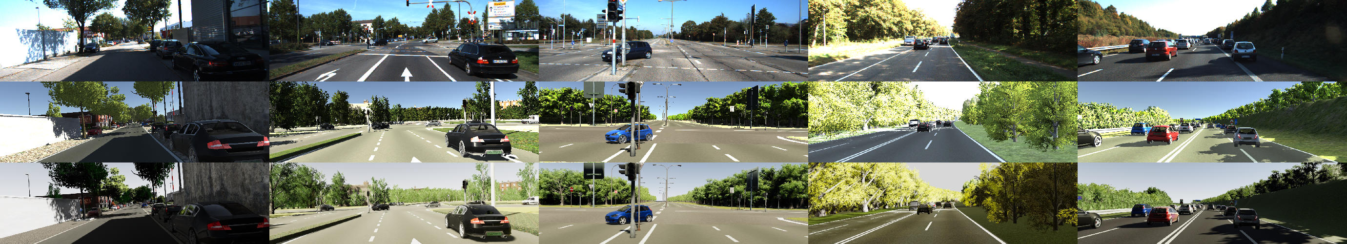
Figure 1: Top row: KITTI images. Middle row: Virtual KITTI 1.3.1 images. Bottom row: Virtual KITTI 2.0 images.

2 Changelog

The original Virtual KITTI dataset was built using the Unity game engine. It used version 5.3 at time of release then 5.5 for updated versions. It mostly used standard shaders to render objects and no post-processing of any kind was applied to the rendered images.

In Virtual KITTI 2, the scenes were upgraded to Unity 2018.4 LTS and all the materials to HDRP/Lit in order to leverage the visual improvements of the High Definition Render Pipeline. The geometry and trajectories were not altered in any way. To increase the application and research field, we added a stereo camera.

To generate the modalities of Virtual KITTI 2, we reused the code we wrote to generate the Virtual Gallery Dataset [6] which includes handling of multiple cameras and post-processing of RGB images (supports custom anti-aliasing and the game engine’s post processing package). We extended it by adding Virtual KITTI’s optical flow implementation.

In all, Virtual KITTI 2 contains the same 5 sequence clones as Virtual KITTI but now provides images from a stereo camera (new). Camera 0 is identical to the Virtual KITTI camera, and camera 1 is 0.532725m to its right. Each camera renders RGB, class segmentation, instance segmentation, depth, forward and backward optical flow (new), and forward and backward scene flow images (new). For each sequence, cameras parameters, vehicle color, pose and bounding boxes are provided.

3 Related datasets

In recent years multiple large-scale datasets have been released that focus on furthering appearance and geometry understanding in road scenes. The widely-used Cityscapes [7] dataset contains more than 25k images along with ground-truth semantic segmentation annotations and has been widely used to train and test segmentation models. The SYNTHIA dataset [4, 8, 9] is a synthetic dataset that, similar to Virtual KITTI, was generated using a video game engine. SYNTHIA annotations are focused on semantic segmentation [4] and have been successfully used, in combination with real-world data, to improve segmentation model performance. DrivingStereo [3] is a large-scale real-world dataset designed for the stereo matching problem. Playing for Benchmarks [10] is another synthetically generated dataset which provides a rich selection of data modalities. Virtual Gallery [6] is a synthetic dataset generated to target specific challenges of visual localization such as illumination changes or occlusions. An interesting collection of datasets can be found here. In a complementary line of work, a method was proposed for validating that a selected dataset is relevant for a given task and contains sufficient variability  [11, 12].

Virtual KITTI is unique in that it can be applied to the union of problems addressable by each of the datasets cited above. More importantly, Virtual KITTI is a reproduction of camera sequences captured in real environments which additionally enables research on domain adaptation, both from sim2real and between different camera angles, filming conditions, and environments [13].

4 Experiments

4.1 Multi-Object Tracking

In a first set of experiments, we attempted to reproduce the conclusion in [1], which is that in the context of multi-object tracking performance the gap between real and virtual data is small.

In [1], transferability was tested by comparing multi-object tracking metrics between real and virtual worlds. In particular, a pre-trained Fast-RCNN [14] model was used as a detector and combined with edge boxes proposals [15]. Two trackers were then evaluated, the dynamic programming min-cost flow (DP-MCF) algorithm of Pirsiavash et al. [16] and the Markov Decision Process (MDP) method of Xiang et al. [17]. They used Bayesian hyperparameter optimization [18] to find fixed tracker hyperparameters for each pair of real and clone videos with the sum of the multi-object tracking accuracies [19] as the objective function.

In this paper, real KITTI videos are compared to Virtual KITTI 1.3.1 and Virtual KITTI 2. Faster-RCNN [20] (PyTorch implementation [21]) replaces Fast-RCNN/Edge Boxes proposals. ResNet-50 FPN[22][23] was used as the backbone. Similar to the original experiment, the network was first trained on imagenet, then fine-tuned on pascal voc 2007 [24] and finally on the KITTI object detection benchmark  [5].

The results are reported in table 1. In this experiment, we show that for every pair there exists a set of DP-MCF parameters for which the MOTA metrics are high and similar between real and virtual data. The conclusions of the original paper therefore still apply.

Table 1: DP-MCF MOT results on original real-world KITTI train videos and virtual world video “clones” (prefixed by a “v”). real vs 1.31 (left) and real vs 2.0 (right). AVG (resp. v-AVG) is the average over real (resp. virtual) sequences. We report the CLEAR MOT metrics [19] – including MOT Accuracy (MOTA), MOT Precision (MOTP), ID Switches (I), and Fragmentation (F) – complemented by the Mostly Tracked (MT) and Mostly Lost (ML) ratios, precision (P) and recall (R).

DPMCF	MOTA$\uparrow$	MOTP$\uparrow$	MT$\uparrow$	ML$\uparrow$	I$\downarrow$	F$\downarrow$	P$\uparrow$	R$\uparrow$
real 0001	86.3%	90.7%	92.0%	1.3%	22	43	93.6%	95.8%
v1.31 0001	86.5%	81.8%	78.9%	2.8%	10	45	99.5%	89.8%
real 0002	87.3%	88.3%	90.9%	0.0%	0	6	95.6%	92.4%
v1.31 0002	87.4%	81.7%	90.0%	0.0%	1	9	98.5%	89.9%
real 0006	97.3%	90.6%	100.0%	0.0%	4	5	99.7%	98.9%
v1.31 0006	97.2%	88.3%	100.0%	0.0%	2	7	99.7%	98.2%
real 0018	88.6%	92.5%	47.1%	23.5%	0	2	96.5%	92.9%
v1.31 0018	88.5%	69.6%	50.0%	33.3%	0	6	99.8%	89.9%
real 0020	90.9%	91.3%	87.2%	4.7%	28	45	97.3%	95.0%
v1.31 0020	90.9%	79.0%	73.4%	7.4%	5	27	99.3%	92.5%
real AVG	90.1%	90.7%	83.4%	5.9%	11	20	96.5%	95.0%
v1.31-AVG	90.1%	80.1%	78.5%	8.7%	4	19	99.4%	92.1%

DPMCF	MOTA$\uparrow$	MOTP$\uparrow$	MT$\uparrow$	ML$\uparrow$	I$\downarrow$	F$\downarrow$	P$\uparrow$	R$\uparrow$
real 0001	89.9%	90.7%	93.3%	2.7%	26	44	95.0%	97.1%
v2.03 0001	89.1%	84.9%	83.1%	1.3%	12	40	99.9%	91.4%
real 0002	89.8%	88.2%	90.9%	0.0%	2	7	96.5%	94.5%
v2.03 0002	89.8%	82.7%	90.0%	0.0%	1	9	100.0%	90.9%
real 0006	97.3%	90.7%	100.0%	0.0%	2	3	100.0%	98.1%
v2.03 0006	97.3%	86.7%	100.0%	0.0%	3	4	100.0%	98.4%
real 0018	90.9%	92.3%	88.2%	0.0%	3	4	93.4%	99.0%
v2.03 0018	90.8%	75.4%	55.6%	0.0%	4	17	99.4%	92.7%
real 0020	89.4%	91.3%	86.0%	5.8%	40	69	96.7%	94.5%
v2.03 0020	89.1%	83.4%	70.0%	7.0%	19	51	99.5%	91.1%
real AVG	91.5%	90.6%	91.7%	1.7%	15	25	96.3%	96.6%
v2.03-AVG	91.2%	82.6%	79.7%	1.7%	8	24	99.8%	92.9%

For completeness, we also include the results of the variation experiment in table 2. It is noteworthy that the lighting condition changes in Virtual KITTI 2 have a smaller impact on the results. The significantly different implementations of the condition changes make them difficult to compare.

Table 2: Impact of variations on DP-MCF MOT performance in virtual KITTI for the v1.31 (left) and v2.0 (right) versions.

v1.31	MOTA$\uparrow$	MOTP$\uparrow$	MT$\uparrow$	ML$\uparrow$	I$\downarrow$	F$\downarrow$	P$\uparrow$	R$\uparrow$
+15deg	-1.3%	-0.3%	-2.9%	1.5%	-1	-3	-0.3%	-0.7%
+30deg	-3.1%	-1.5%	-12.5%	4.1%	-3	-9	0.3%	-2.4%
-15deg	-0.5%	-0.2%	-2.3%	-1.7%	1	2	-0.3%	-0.3%
-30deg	-3.2%	-0.6%	-6.5%	1.9%	1	-1	-1.2%	-1.8%
morning	-6.4%	-1.3%	-7.0%	5.0%	1	0	-0.2%	-5.5%
sunset	-7.5%	-2.8%	-9.2%	7.2%	0	2	-0.9%	-6.0%
overcast	-4.5%	-2.4%	-5.8%	4.5%	1	1	0.1%	-4.0%
fog	-72.8%	3.1%	-73.8%	63.1%	-3	-13	0.6%	-66.7%
rain	-29.8%	-0.8%	-46.7%	17.8%	0	4	0.3%	-6.0%

v2.0	MOTA$\uparrow$	MOTP$\uparrow$	MT$\uparrow$	ML$\uparrow$	I$\downarrow$	F$\downarrow$	P$\uparrow$	R$\uparrow$
+15deg	-1.1%	-0.1%	-6.8%	1.7%	0	-4	0.0%	-0.7%
+30deg	-1.3%	-1.7%	-13.3%	3.7%	-5	-10	-0.1%	-0.9%
-15deg	-1.1%	0.1%	-0.5%	-0.3%	4	5	-0.7%	0.5%
-30deg	-2.7%	-0.7%	-0.6%	0.7%	3	6	1.3%	-1.4%
morning	-0.9%	-0.3%	-4.5%	0.7%	1	4	0.1%	-0.9%
sunset	-2.5%	-0.5%	-1.7%	1.8%	3	6	0.0%	-2.2%
overcast	-0.3%	-0.6%	2.4%	1.2%	0	3	0.0%	-0.3%
fog	-79.6%	3.5%	-78.6%	75.5%	-7	-22	0.2%	-73.5%
rain	-16.5%	-0.8%	-33.0%	5.7%	-2	13	0.2%	-15.2%

In the next experiment, we evaluated the training performance of the three datasets. We finetuned the pre-trained imagenet model on the 5 cloned KITTI sequences then tuned the detector on 5 short videos (0,3,10,12,14) and finally evaluated the performance on a test set of 7 long diverse videos (4,5,7,8,9,11,15). All three models converged very rapidly (with very few epochs), as shown in Figure 2. Detailed metrics are reported in table 3. In this experiment, the improved RGB seems to have a larger effect closing the gap by 50%.

Table 3: DP-MCF results on seven long diverse real-world KITTI videos (4,5,7,8,9,11,15) by training the models on the five cloned KITTI videos (1,2,6,18,20). Reported results correspond to epoch 13.

	MOTA$\uparrow$	MOTP$\uparrow$	MT$\uparrow$	ML$\uparrow$	I$\downarrow$	F$\downarrow$	P$\uparrow$	R$\uparrow$
real	83.9%	84.3%	67.4%	15.3%	12	24	98.3%	88.3%
v1.31	60.6%	82.1%	30.7%	30.4%	2	8	98.9%	64.3%
v2.0	71.5%	82.9%	43.1%	18.7%	4	20	99.8%	75.1%

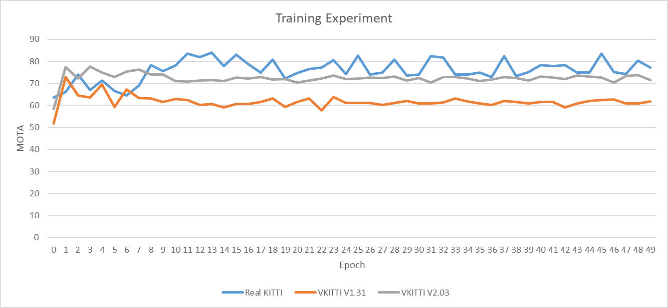
Figure 2: Per epoch MOTA results for the training experiment.

4.2 GANet

Since Virtual KITTI 2 also provides stereo image pairs (contrary to the original version), we conducted experiments with a dense deep learning-based stereo matching method, namely GANet [25]. One of the main advantages of Virtual KITTI 1 & 2 is the ability to test algorithms under different conditions. In detail, we can test algorithms with a configuration as close as possible to the real KITTI dataset (clone) as well as with artificial rain, fog or even with slight changes of camera configurations (e.g. rotated 15 degree left). In order to show these new capabilities, we ran GANet [25] on Virtual KITTI 2 as well as on the real KITTI sequences (KITTI tracking benchmark [5]) using the provided pre-trained models. Figure 3 shows one example disparity map (inverse depth) generated using GANet and Virtual KITTI 2. The ground-truth (the reference data provided with our dataset) can be found in the middle and the synthetic camera image can be found at the top. Tables 4 and 5 show qualitative results of GANet on the real KITTI sequence (real) and Virtual KITTI 2 (all others). There are two main findings: (i) Our clone of the real sequence performs similarly to the real sequence. (ii) Only fog and rain significantly decrease the stereo matching results using this algorithm. Since the original Virtual KITTI does not provide stereo images, we could not run GANet for comparison.

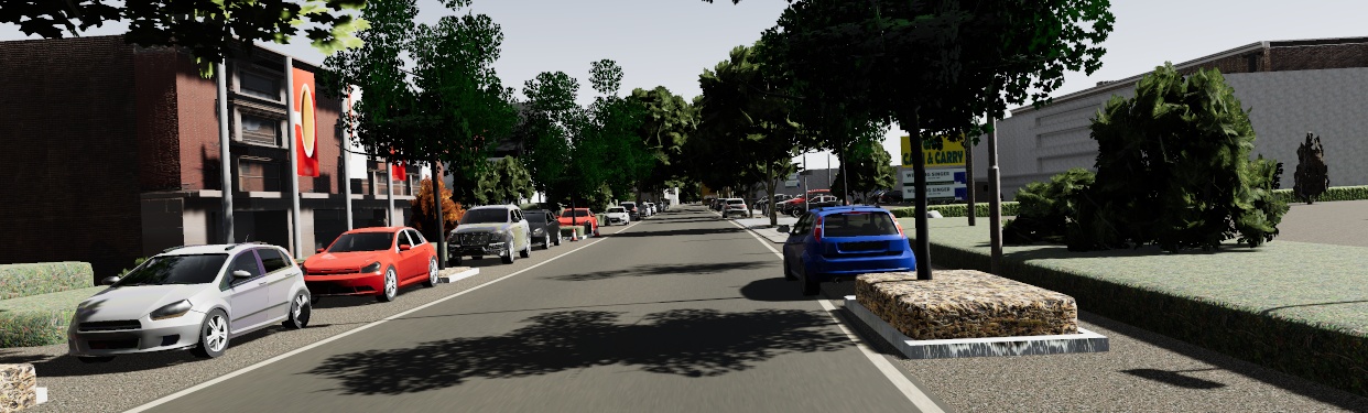
(a)

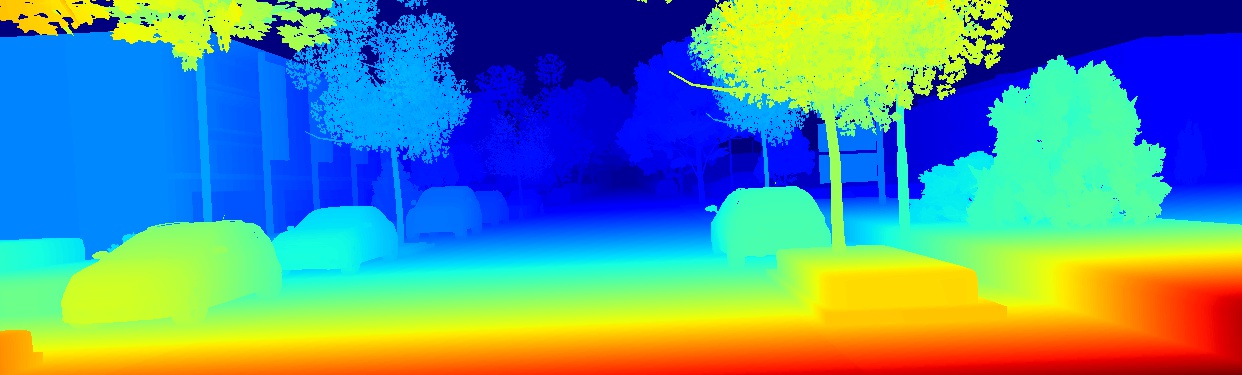
(b)

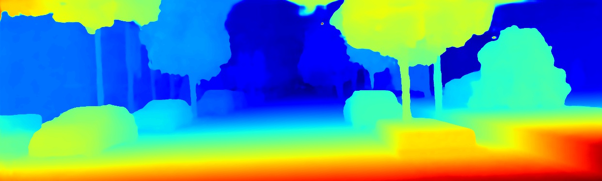
(c)

Figure 3: Example image from scene 01: a) RGB image, b) ground-truth disparity map, c) disparity map from GANet (using pre-trained model).

Table 4: Average error in pixels using the GANet model kitti2015_final and an error threshold of 1 pixel.

condition	scene01	scene02	scene06	scene18	scene20
real	1.6421	0.7552	1.2111	2.4188	1.5800
clone	0.9915	0.8674	0.9201	1.7671	1.0145
fog	1.4277	1.0595	1.0789	2.0343	1.5217
morning	1.0374	0.8401	0.9568	1.7454	1.3149
overcast	0.9615	0.7892	0.9634	1.8469	1.0638
rain	1.4500	1.2255	1.2010	1.9652	1.3850
sunset	1.0077	0.8336	0.9836	1.7923	1.2003
15-deg-left	0.9118	0.9677	0.8344	1.4555	1.2785
15-deg-right	1.0643	0.9232	1.0183	2.2778	0.7809
30-deg-left	0.9811	0.9439	0.8409	1.2944	1.6015
30-deg-right	1.2312	0.9529	0.9061	3.0761	0.6355

Table 5: Error rate in percent using the GANet model kitti2015_final.

condition	scene01	scene02	scene06	scene18	scene20
real	0.1579	0.1041	0.0853	0.2336	0.2228
clone	0.1259	0.1420	0.1058	0.2831	0.1427
fog	0.2010	0.2028	0.1442	0.3257	0.2271
morning	0.1407	0.1354	0.1048	0.2809	0.1457
overcast	0.1208	0.1129	0.1038	0.3027	0.1415
rain	0.1851	0.1818	0.1806	0.3303	0.1878
sunset	0.1324	0.1336	0.1140	0.2871	0.1381
15-deg-left	0.1298	0.1448	0.0948	0.2718	0.1675
15-deg-right	0.1271	0.1386	0.1096	0.3051	0.1171
30-deg-left	0.1436	0.1392	0.0896	0.2717	0.1927
30-deg-right	0.1334	0.1426	0.1177	0.3599	0.0964

4.3 SfmLearner

In this experiment, we ran a deep learning-based monocular depth and camera pose estimation algorithm on Virtual KITTI 1 and 2 as well as on the real sequences which were used to generate Virtual KITTI (KITTI tracking benchmark [5]). We selected a method called SfmLearner [26] (PyTorch implementation) and used the pre-trained model provided by the authors for all experiments. Tables 6 - 9 show the results on depth estimation using SfmLearner on both versions of Virtual KITTI as well as real KITTI (real) on scene 01 and scene 02.

Table 6: Results of depth/disparity estimation using the SfmLearner model kitti_orig on scene 01 of Virtual KITTI 1.3.1.

configuration	abs_diff$\downarrow$	abs_rel$\downarrow$	sq_rel$\downarrow$	rms$\downarrow$	log_rms$\downarrow$	abs_log$\downarrow$	a1$\uparrow$	a2$\uparrow$	a3$\uparrow$
real	4.1299	0.1871	1.6941	7.6553	0.2969	0.1997	0.7110	0.8765	0.9333
clone	4.3969	0.1978	1.9045	8.5235	0.3056	0.2086	0.6953	0.8606	0.9453
fog	7.3598	0.3156	4.2483	13.3553	0.5175	0.3755	0.4597	0.7190	0.8245
morning	4.9541	0.2196	2.2166	9.2157	0.3326	0.2349	0.6496	0.8322	0.9270
overcast	4.9401	0.2216	2.1929	9.2519	0.3331	0.2363	0.6346	0.8355	0.9304
rain	5.3665	0.2327	2.5394	10.2340	0.3656	0.2554	0.6239	0.8116	0.9097
sunset	5.0265	0.2239	2.2690	9.4546	0.3463	0.2430	0.6377	0.8308	0.9248
15-deg-left	5.5871	0.2962	3.4072	10.0035	0.4023	0.2855	0.5704	0.7752	0.8869
15-deg-right	5.2487	0.2539	2.6596	9.6428	0.3728	0.2622	0.6079	0.8035	0.9111
30-deg-left	6.3031	0.3538	4.4495	10.9083	0.4579	0.3333	0.5120	0.7367	0.8495
30-deg-right	6.2300	0.3182	3.7206	11.1724	0.4436	0.3209	0.5131	0.7553	0.8674

Table 7: Results of depth/disparity estimation using the SfmLearner model kitti_orig on scene 01 of Virtual KITTI 2.

configuration	abs_diff$\downarrow$	abs_rel$\downarrow$	sq_rel$\downarrow$	rms$\downarrow$	log_rms$\downarrow$	abs_log$\downarrow$	a1$\uparrow$	a2$\uparrow$	a3$\uparrow$
real	4.1299	0.1871	1.6941	7.6553	0.2969	0.1997	0.7110	0.8765	0.9333
clone	4.1806	0.2006	1.8738	8.0914	0.2987	0.2048	0.7053	0.8827	0.9502
fog	7.6199	0.3590	4.6061	13.3686	0.5464	0.4074	0.4120	0.6748	0.8048
morning	4.7793	0.2510	2.2305	8.3154	0.3333	0.2479	0.5803	0.8410	0.9386
overcast	4.8226	0.2312	2.2000	8.9075	0.3222	0.2352	0.6343	0.8489	0.9336
rain	6.0536	0.2788	3.1175	10.9652	0.4119	0.3037	0.5267	0.7786	0.8813
sunset	4.5673	0.2380	2.0761	8.3144	0.3275	0.2371	0.6190	0.8517	0.9397
15-deg-left	4.1439	0.1881	1.8862	8.0820	0.2901	0.1933	0.7233	0.8871	0.9478
15-deg-right	4.5730	0.2352	2.2298	8.7058	0.3312	0.2348	0.6383	0.8428	0.9311
30-deg-left	4.2628	0.2027	2.1297	8.4016	0.3053	0.2038	0.7037	0.8733	0.9411
30-deg-right	4.9444	0.2829	2.7174	9.5778	0.3784	0.2747	0.5799	0.7915	0.8969

Table 8: Results of depth/disparity estimation using the SfmLearner model kitti_orig on scene 02 of Virtual KITTI 1.3.1.

configuration	abs_diff$\downarrow$	abs_rel$\downarrow$	sq_rel$\downarrow$	rms$\downarrow$	log_rms$\downarrow$	abs_log$\downarrow$	a1$\uparrow$	a2$\uparrow$	a3$\uparrow$
real	2.8982	0.1080	0.9600	6.3456	0.1931	0.1151	0.8665	0.9522	0.9834
clone	5.1034	0.1574	2.1665	10.6132	0.2861	0.1800	0.7687	0.8747	0.9415
fog	8.2950	0.2741	4.8755	15.8891	0.5288	0.3545	0.5552	0.7586	0.8290
morning	5.7313	0.1835	2.6022	11.3875	0.3225	0.2104	0.7188	0.8452	0.9223
overcast	5.7112	0.1867	2.6115	11.3082	0.3241	0.2124	0.7156	0.8454	0.9290
rain	7.2143	0.2311	3.7951	14.0354	0.4290	0.2856	0.6303	0.7837	0.8638
sunset	6.0525	0.1892	2.9137	12.2815	0.3568	0.2260	0.7211	0.8368	0.8997
15-deg-left	5.9324	0.1918	2.9228	11.8774	0.3470	0.2179	0.7144	0.8304	0.9073
15-deg-right	5.7166	0.1994	2.7859	11.0579	0.3299	0.2159	0.7149	0.8458	0.9230
30-deg-left	6.4106	0.1955	3.3892	13.1429	0.3873	0.2349	0.7074	0.8243	0.8826
30-deg-right	5.7453	0.2084	2.8659	10.9117	0.3291	0.2195	0.6997	0.8424	0.9266

Table 9: Results of depth/disparity estimation using the SfmLearner model kitti_orig on scene 02 of Virtual KITTI 2.

configuration	abs_diff$\downarrow$	abs_rel$\downarrow$	sq_rel$\downarrow$	rms$\downarrow$	log_rms$\downarrow$	abs_log$\downarrow$	a1$\uparrow$	a2$\uparrow$	a3$\uparrow$
real	2.8982	0.1080	0.9600	6.3456	0.1931	0.1151	0.8665	0.9522	0.9834
clone	6.9450	0.2261	3.6433	13.6930	0.4249	0.2818	0.6278	0.7979	0.8717
fog	8.1171	0.2749	4.7223	15.6484	0.5196	0.3496	0.5383	0.7695	0.8380
morning	7.0506	0.2129	3.8568	14.3007	0.4326	0.2720	0.6737	0.7971	0.8675
overcast	4.9188	0.1694	2.0306	9.8010	0.2762	0.1839	0.7433	0.8855	0.9570
rain	6.5200	0.2155	3.1826	12.8214	0.3815	0.2567	0.6521	0.8159	0.8910
sunset	5.2766	0.1623	2.5095	11.0582	0.3116	0.1864	0.7549	0.8585	0.9246
15-deg-left	6.1858	0.2070	2.9970	12.2804	0.3737	0.2495	0.6721	0.8199	0.8980
15-deg-right	7.3299	0.2577	4.1986	14.3245	0.4733	0.3194	0.5724	0.7482	0.8411
30-deg-left	5.7392	0.1957	2.6946	11.5449	0.3479	0.2294	0.7038	0.8309	0.9204
30-deg-right	6.0436	0.2476	3.3457	12.1962	0.4322	0.2896	0.6127	0.7747	0.8635

Tables 10 and 11 show the results of camera pose estimation using the metric absolute translation error (ATE) for Virtual KITTI 1.3.1 and 2. The rotation error (RE) for both Virtual KITTI versions is given in tables 12 and 13.

Table 10: Results of camera pose estimation (ATE, absolute translation error, mean (std)) using the SfmLearner model kitti_orig on all scenes of Virtual KITTI 1.3.1.

condition	scene01	scene02	scene06	scene18	scene20
real	0.0211 (0.0136)	0.0124 (0.0117)	0.0045 (0.0064)	0.0143 (0.0081)	0.0184 (0.0086)
clone	0.0207 (0.0130)	0.0125 (0.0118)	0.0067 (0.0108)	0.0148 (0.0086)	0.0204 (0.0118)
fog	0.0263 (0.0170)	0.0180 (0.0213)	0.0081 (0.0169)	0.0213 (0.0165)	0.0227 (0.0157)
morning	0.0217 (0.0131)	0.0119 (0.0109)	0.0062 (0.0093)	0.0155 (0.0099)	0.0181 (0.0110)
overcast	0.0215 (0.0133)	0.0131 (0.0121)	0.0062 (0.0091)	0.0160 (0.0108)	0.0186 (0.0105)
rain	0.0223 (0.0135)	0.0141 (0.0134)	0.0059 (0.0093)	0.0167 (0.0103)	0.0214 (0.0117)
sunset	0.0212 (0.0127)	0.0135 (0.0123)	0.0056 (0.0080)	0.0155 (0.0096)	0.0180 (0.0092)
15-deg-left	0.2063 (0.1145)	0.1377 (0.1438)	0.0480 (0.0814)	0.2019 (0.1282)	0.2315 (0.1167)
15-deg-right	0.1856 (0.0953)	0.1240 (0.1265)	0.0532 (0.0885)	0.1954 (0.1142)	0.2228 (0.1090)
30-deg-left	0.3832 (0.2078)	0.2561 (0.2667)	0.0960 (0.1624)	0.3810 (0.2315)	0.4423 (0.2175)
30-deg-right	0.3611 (0.1879)	0.2464 (0.2541)	0.0991 (0.1661)	0.3688 (0.2154)	0.4309 (0.2115)

Table 11: Results of camera pose estimation (ATE, absolute translation error, mean (std)) using the SfmLearner model kitti_orig on all scenes of Virtual KITTI 2.

condition	scene01	scene02	scene06	scene18	scene20
real	0.0211 (0.0136)	0.0124 (0.0117)	0.0045 (0.0064)	0.0143 (0.0081)	0.0184 (0.0086)
clone	0.0212 (0.0130)	0.0123 (0.0112)	0.0066 (0.0107)	0.0146 (0.0091)	0.0197 (0.0114)
fog	0.0253 (0.0163)	0.0147 (0.0147)	0.0060 (0.0101)	0.0204 (0.0151)	0.0222 (0.0124)
morning	0.0220 (0.0133)	0.0110 (0.0093)	0.0056 (0.0082)	0.0162 (0.0102)	0.0183 (0.0109)
overcast	0.0216 (0.0129)	0.0119 (0.0111)	0.0051 (0.0074)	0.0168 (0.0106)	0.0194 (0.0111)
rain	0.0233 (0.0141)	0.0134 (0.0123)	0.0058 (0.0087)	0.0173 (0.0120)	0.0219 (0.0118)
sunset	0.0207 (0.0128)	0.0123 (0.0114)	0.0049 (0.0070)	0.0163 (0.0111)	0.0189 (0.0094)
15-deg-left	0.2060 (0.1143)	0.1368 (0.1424)	0.0478 (0.0807)	0.2029 (0.1284)	0.2309 (0.1169)
15-deg-right	0.1857 (0.0950)	0.1241 (0.1266)	0.0531 (0.0885)	0.1937 (0.1148)	0.2266 (0.1092)
30-deg-left	0.3826 (0.2075)	0.2557 (0.2663)	0.0956 (0.1616)	0.3829 (0.2313)	0.4422 (0.2177)
30-deg-right	0.3616 (0.1878)	0.2454 (0.2531)	0.0987 (0.1654)	0.3695 (0.2152)	0.4358 (0.2133)

Table 12: Results of camera pose estimation (RE, rotation error, mean (std)) using the SfmLearner model kitti_orig on all scenes of Virtual KITTI 1.3.1.

condition	scene01	scene02	scene06	scene18	scene20
real	0.0028 (0.0017)	0.0016 (0.0011)	0.0026 (0.0037)	0.0018 (0.0009)	0.0028 (0.0021)
clone	0.0027 (0.0018)	0.0017 (0.0008)	0.0026 (0.0026)	0.0026 (0.0010)	0.0024 (0.0013)
fog	0.0076 (0.0102)	0.0141 (0.0152)	0.0151 (0.0157)	0.0050 (0.0041)	0.0083 (0.0066)
morning	0.0028 (0.0018)	0.0021 (0.0008)	0.0027 (0.0034)	0.0017 (0.0007)	0.0025 (0.0017)
overcast	0.0029 (0.0020)	0.0019 (0.0008)	0.0027 (0.0029)	0.0022 (0.0010)	0.0021 (0.0015)
rain	0.0035 (0.0029)	0.0058 (0.0046)	0.0081 (0.0078)	0.0022 (0.0011)	0.0057 (0.0035)
sunset	0.0033 (0.0033)	0.0020 (0.0008)	0.0030 (0.0030)	0.0019 (0.0007)	0.0023 (0.0015)
15-deg-left	0.0084 (0.0047)	0.0045 (0.0044)	0.0036 (0.0044)	0.0056 (0.0031)	0.0057 (0.0049)
15-deg-right	0.0086 (0.0059)	0.0045 (0.0041)	0.0035 (0.0044)	0.0072 (0.0023)	0.0061 (0.0033)
30-deg-left	0.0212 (0.0130)	0.0105 (0.0117)	0.0053 (0.0081)	0.0169 (0.0102)	0.0123 (0.0116)
30-deg-right	0.0205 (0.0126)	0.0085 (0.0093)	0.0070 (0.0083)	0.0210 (0.0094)	0.0160 (0.0082)

Table 13: Results of camera pose estimation (RE, rotation error, mean (std)) using the SfmLearner model kitti_orig on all scenes of Virtual KITTI 2.

condition	scene01	scene02	scene06	scene18	scene20
real	0.0028 (0.0017)	0.0016 (0.0011)	0.0026 (0.0037)	0.0018 (0.0009)	0.0028 (0.0021)
clone	0.0027 (0.0018)	0.0017 (0.0008)	0.0030 (0.0036)	0.0020 (0.0008)	0.0020 (0.0010)
fog	0.0069 (0.0077)	0.0099 (0.0089)	0.0110 (0.0100)	0.0040 (0.0030)	0.0082 (0.0067)
morning	0.0032 (0.0023)	0.0019 (0.0009)	0.0028 (0.0029)	0.0018 (0.0008)	0.0023 (0.0020)
overcast	0.0029 (0.0020)	0.0019 (0.0008)	0.0027 (0.0023)	0.0017 (0.0008)	0.0024 (0.0016)
rain	0.0037 (0.0028)	0.0064 (0.0058)	0.0064 (0.0047)	0.0032 (0.0022)	0.0060 (0.0032)
sunset	0.0036 (0.0046)	0.0018 (0.0008)	0.0025 (0.0027)	0.0018 (0.0007)	0.0020 (0.0012)
15-deg-left	0.0086 (0.0051)	0.0044 (0.0042)	0.0040 (0.0055)	0.0055 (0.0027)	0.0062 (0.0046)
15-deg-right	0.0089 (0.0059)	0.0046 (0.0045)	0.0034 (0.0042)	0.0064 (0.0023)	0.0054 (0.0033)
30-deg-left	0.0219 (0.0133)	0.0105 (0.0120)	0.0056 (0.0088)	0.0167 (0.0102)	0.0134 (0.0115)
30-deg-right	0.0214 (0.0139)	0.0090 (0.0101)	0.0062 (0.0073)	0.0204 (0.0102)	0.0134 (0.0082)

4.4 Semantic segmentation

In this section we use Virtual KITTI 2’s ground-truth semantic segmentation annotations to evaluate a state-of-the-art urban scene segmentation method, Adapnet++ [27], under Virtual KITTI 2 variations. We use the pre-trained models provided by the authors. These models were trained using the CityScapes [7] dataset. The models were trained on 11 semantic categories from CityScapes. We evaluated on the following 7 classes (in addition to background) which were the classes common to both Virtual KITTI 2 and CityScapes: sky, building, road, vegetation, pole, car/truck/bus, and traffic sign. We evaluate on both RGB and depth input settings. While we would have ideally liked to have used models trained on real KITTI data, there currently exists only a small set of 200 KITTI images with segmentation data. Further, because these 200 images do not correspond to an image sequence, we do not have a cloned virtual sequence with which to compare.

Table 14 shows mAP of the Adapnet++ model trained on RGB images and tested on Virtual KITTI 2. One sees similar performance variations as for the earlier problems addressed. In particular, performance is relatively stable for small and moderate changes in the camera angle (15 and 30 degrees respectively) but degrades significantly in the presence of fog and rain. Table 15 shows results for Adapnet++ model trained on depth images. We first note that semantic segmentation performance is in general poorer when using depth images rather than RGB images, which is consistent with [27]. Further, because Virtual KITTI 2’s ground-truth depth is not affected by meteorological conditions or lighting, the depth images for the fog, morning, overcast, rain and sunset variations are identical, and therefore so is the performance of the model. As a point of comparison to real-world data, we evaluated the Adapnet++ RGB model on the 200 KITTI images with segmentation ground-truth. The mAP of 58.07 is in line with the average mAP across the 5 cloned scenes of 58.22. This indicates that Virtual KITTI 2 may be a good proxy dataset for evaluating segmentation algorithms on KITTI. Figure 4 shows examples of segmentation results for both RGB and depth frames. We can see that the RGB model performs well overall while the depth model often confuses the sky and building classes.

Table 14: RGB semantic segmentation mAP results for different variations of Virtual KITTI 2.

condition	scene01	scene02	scene06	scene18	scene20
clone	75.47	53.28	61.46	29.71	71.20
fog	44.89	34.75	43.39	46.80	48.11
morning	64.41	24.08	47.01	20.10	58.03
overcast	68.36	60.19	58.95	32.49	71.55
rain	48.77	44.74	45.15	39.56	52.47
sunset	59.59	47.90	55.22	30.95	51.37
15-deg-left	70.64	59.06	68.13	28.98	69.94
15-deg-right	74.05	46.73	60.37	31.61	71.63
30-deg-left	68.82	55.22	69.46	28.83	66.20
30-deg-right	70.49	44.63	57.11	30.72	71.03

Table 15: Depth semantic segmentation mAP results for different variations of Virtual KITTI 2.

condition	scene01	scene02	scene06	scene18	scene20
clone	44.57	34.75	40.84	37.56	34.24
fog	44.57	34.38	40.84	37.56	34.24
morning	44.57	34.75	40.84	37.56	34.24
overcast	44.57	34.38	40.84	37.56	34.24
rain	44.57	34.38	40.84	37.56	34.24
sunset	44.57	34.75	40.84	37.56	34.24
15-deg-left	42.86	32.99	43.40	40.40	30.82
15-deg-right	44.36	33.60	38.60	35.45	34.13
30-deg-left	37.82	30.97	40.07	39.32	26.18
30-deg-right	43.60	29.73	35.50	27.66	33.21

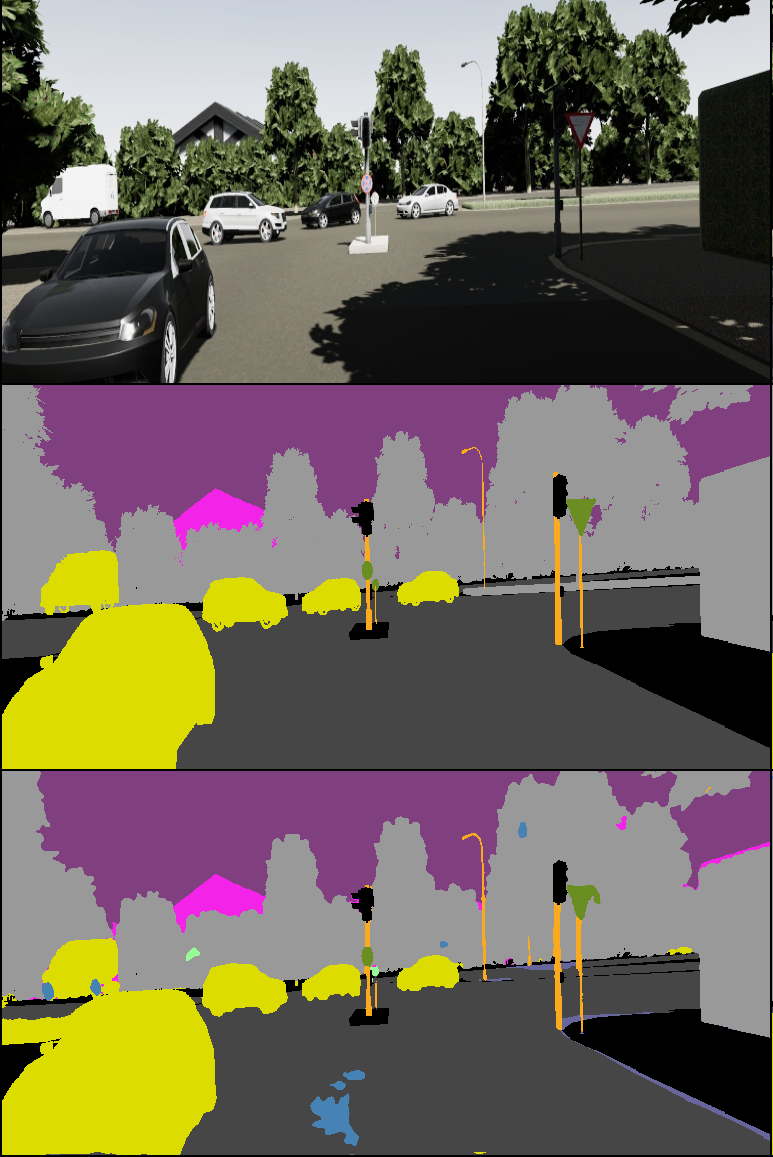
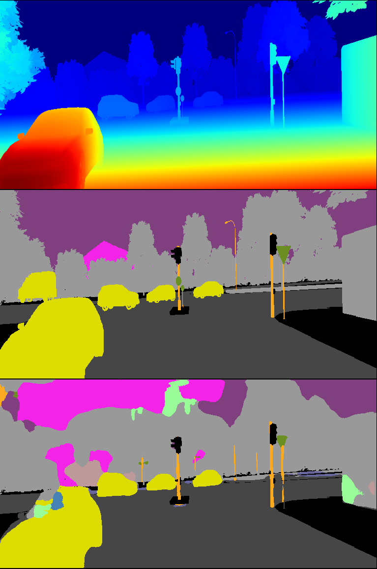
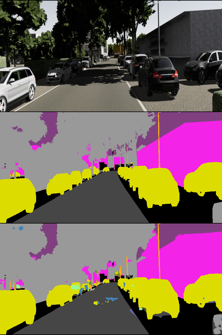
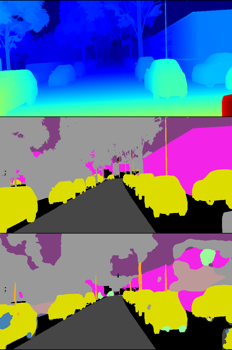
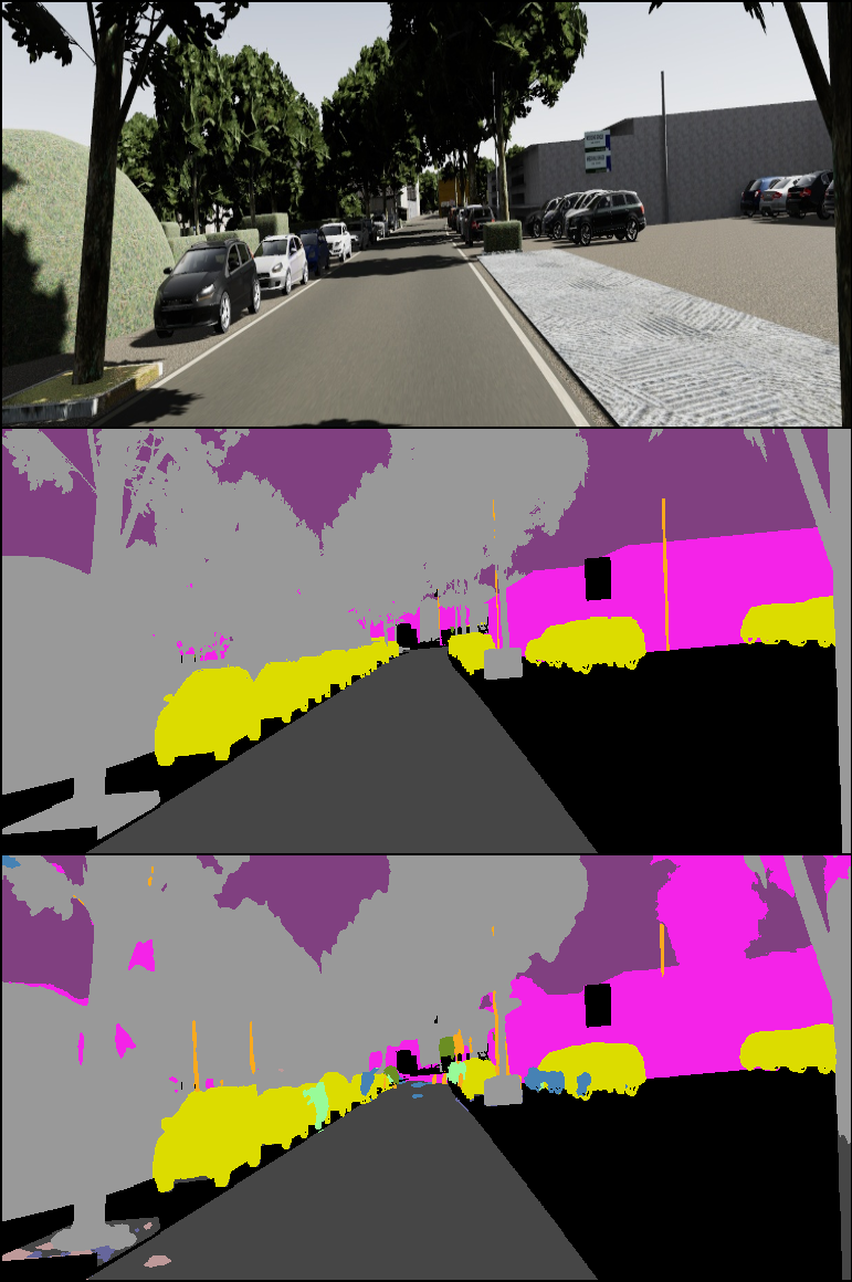
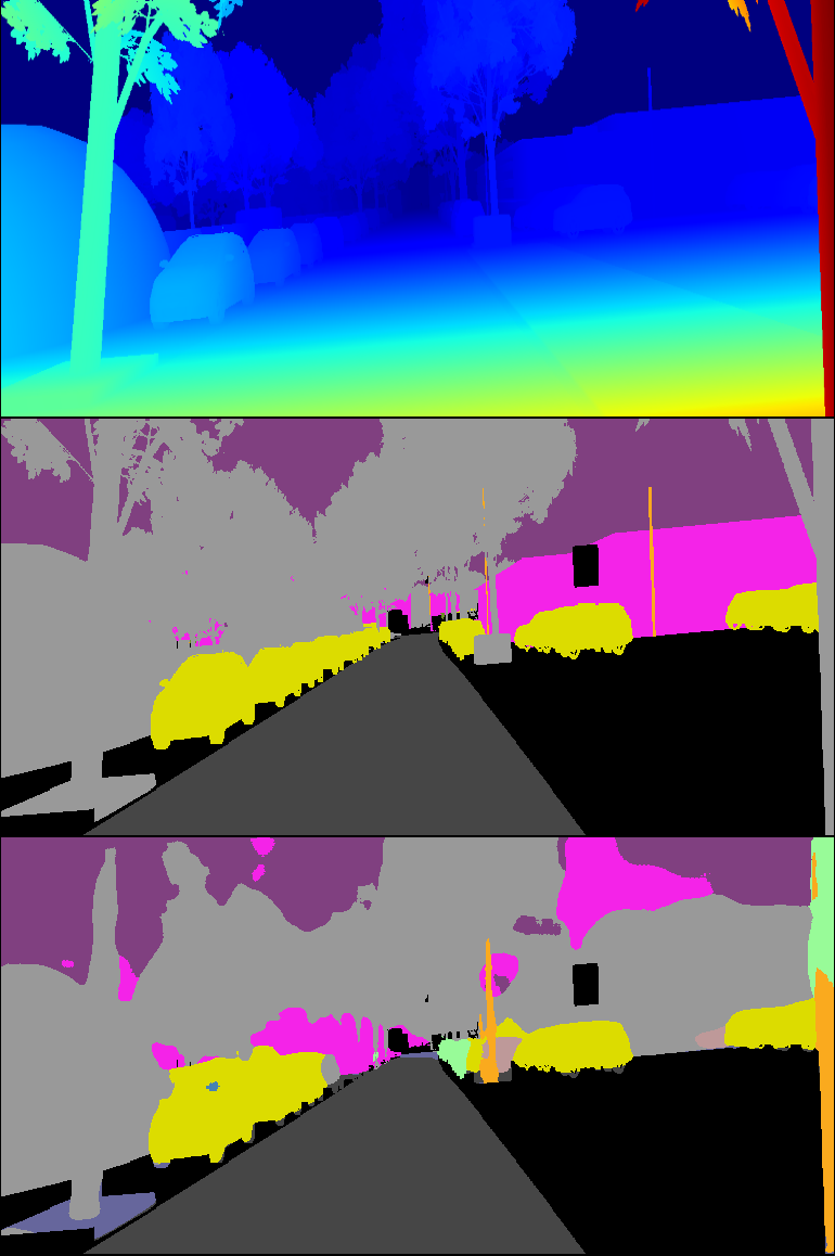
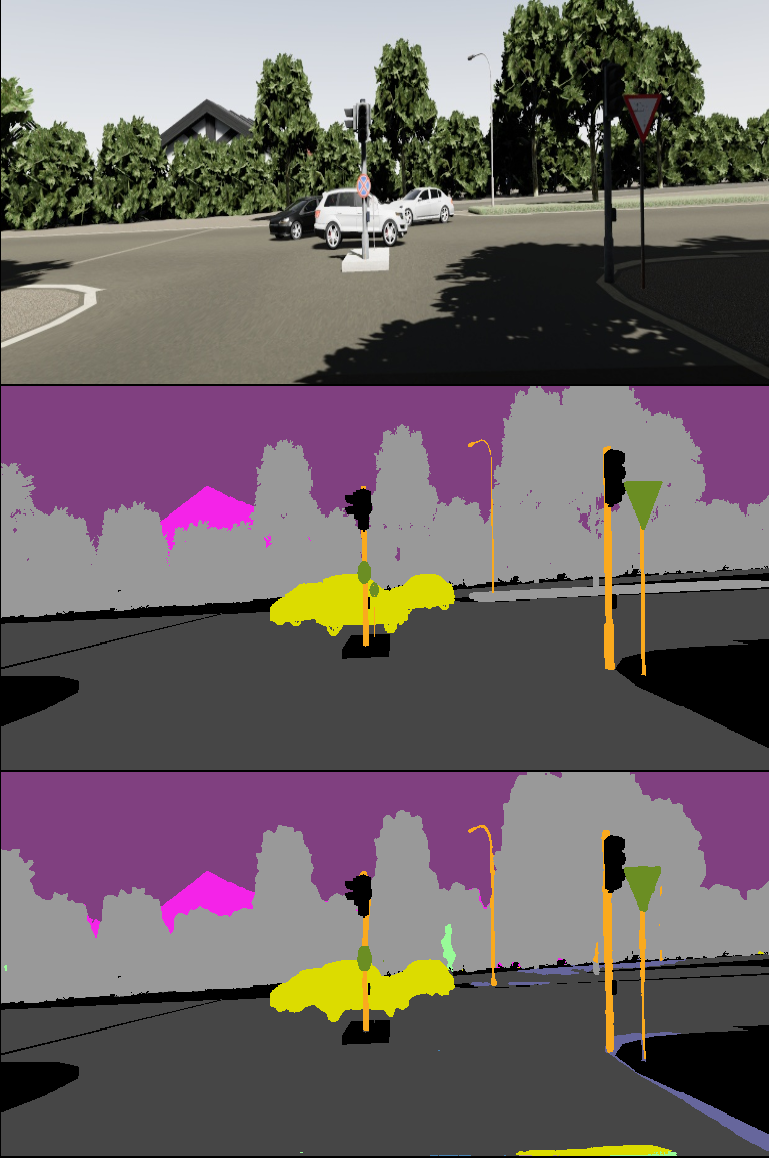
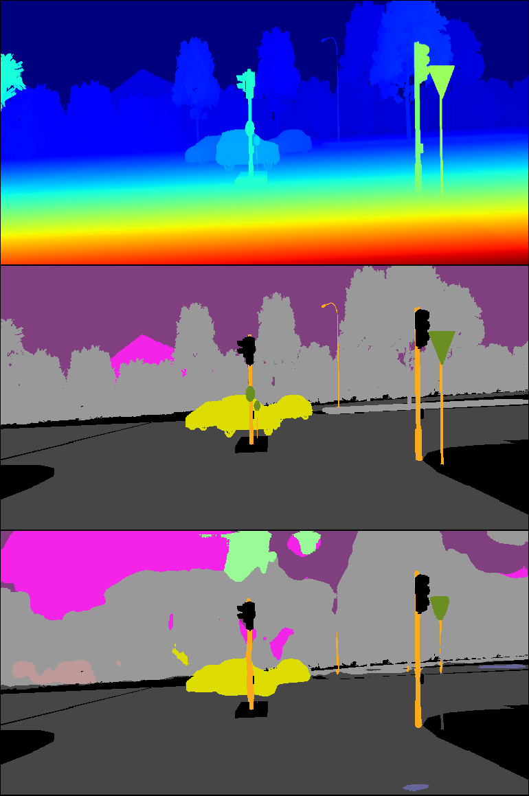
Figure 4: Example RGB-depth pairs and segmentation results. Each image block shows (i) top: input frame (either RGB or depth); (ii) ground-truth; and (iii) predicted segmentation.

References

- [1] A Gaidon, Q Wang, Y Cabon, and E Vig. Virtual worlds as proxy for multi-object tracking analysis. In CVPR, 2016.
- [2] C R De Souza, A Gaidon, Y Cabon, and A M Lopez Pena. Procedural generation of videos to train deep action recognition networks. In CVPR, 2017.
- [3] Guorun Yang, Xiao Song, Chaoqin Huang, Zhidong Deng, Jianping Shi, and Bolei Zhou. Drivingstereo: A large-scale dataset for stereo matching in autonomous driving scenarios. In CVPR, 2019.
- [4] German Ros, Laura Sellart, Joanna Materzynska, David Vazquez, and Antonio M. Lopez. The synthia dataset: A large collection of synthetic images for semantic segmentation of urban scenes. In CVPR, June 2016.
- [5] Andreas Geiger, Philip Lenz, and Raquel Urtasun. Are we ready for autonomous driving? the kitti vision benchmark suite. In Conference on Computer Vision and Pattern Recognition (CVPR), 2012.
- [6] Philippe Weinzaepfel, Gabriela Csurka, Yohann Cabon, and Martin Humenberger. Visual localization by learning objects-of-interest dense match regression. In CVPR, 2019.
- [7] Marius Cordts, Mohamed Omran, Sebastian Ramos, Timo Rehfeld, Markus Enzweiler, Rodrigo Benenson, Uwe Franke, Stefan Roth, and Bernt Schiele. The cityscapes dataset for semantic urban scene understanding. In CVPR, 2016.
- [8] Daniel Hernandez-Juarez, Lukas Schneider, Antonio Espinosa, David Vazquez, Antonio M. Lopez, Uwe Franke, Marc Pollefeys, and Juan Carlos Moure. Slanted stixels: Representing san francisco’s steepest streets. In BMVC, 2017.
- [9] Javad Zolfaghari Bengar, Abel Gonzalez-Garcia, Gabriel Villalonga, Bogdan Raducanu, Hamed H Aghdam, Mikhail Mozerov, Antonio M Lopez, and Joost van de Weijer. Temporal coherence for active learning in videos. In ICCV Workshops, 2019.
- [10] Stephan R Richter, Zeeshan Hayder, and Vladlen Koltun. Playing for benchmarks. In ICCV, pages 2213–2222, 2017.
- [11] Oliver Zendel, Katrin Honauer, Markus Murschitz, Martin Humenberger, and Gustavo Fernandez Dominguez. Analyzing computer vision data-the good, the bad and the ugly. In CVPR, 2017.
- [12] Oliver Zendel, Markus Murschitz, Martin Humenberger, and Wolfgang Herzner. How good is my test data? introducing safety analysis for computer vision. International Journal of Computer Vision, 125(1-3):95–109, 2017.
- [13] Gabriela Csurka. Domain adaptation in computer vision applications. Springer, 2017.
- [14] Ross Girshick. Fast r-cnn. In Proceedings of the IEEE international conference on computer vision, pages 1440–1448, 2015.
- [15] C Lawrence Zitnick and Piotr Dollár. Edge boxes: Locating object proposals from edges. In European conference on computer vision, pages 391–405. Springer, 2014.
- [16] Hamed Pirsiavash, Deva Ramanan, and Charless C Fowlkes. Globally-optimal greedy algorithms for tracking a variable number of objects. In CVPR 2011, pages 1201–1208. IEEE, 2011.
- [17] Yu Xiang, Alexandre Alahi, and Silvio Savarese. Learning to track: Online multi-object tracking by decision making. In Proceedings of the IEEE international conference on computer vision, pages 4705–4713, 2015.
- [18] James Bergstra, Daniel Yamins, and David Daniel Cox. Making a science of model search: Hyperparameter optimization in hundreds of dimensions for vision architectures. 2013.
- [19] Keni Bernardin and Rainer Stiefelhagen. Evaluating multiple object tracking performance: the clear mot metrics. Journal on Image and Video Processing, 2008:1, 2008.
- [20] Shaoqing Ren, Kaiming He, Ross B. Girshick, and Jian Sun. Faster R-CNN: towards real-time object detection with region proposal networks. CoRR, abs/1506.01497, 2015.
- [21] Adam Paszke, Sam Gross, Soumith Chintala, Gregory Chanan, Edward Yang, Zachary DeVito, Zeming Lin, Alban Desmaison, Luca Antiga, and Adam Lerer. Automatic differentiation in PyTorch. In NIPS Autodiff Workshop, 2017.
- [22] Kaiming He, Xiangyu Zhang, Shaoqing Ren, and Jian Sun. Deep residual learning for image recognition. CoRR, abs/1512.03385, 2015.
- [23] Tsung-Yi Lin, Piotr Dollár, Ross B. Girshick, Kaiming He, Bharath Hariharan, and Serge J. Belongie. Feature pyramid networks for object detection. CoRR, abs/1612.03144, 2016.
- [24] M. Everingham, L. Van Gool, C. K. I. Williams, J. Winn, and A. Zisserman. The PASCAL Visual Object Classes Challenge 2007 (VOC2007) Results. http://www.pascal-network.org/challenges/VOC/voc2007/workshop/index.html.
- [25] Feihu Zhang, Victor Prisacariu, Ruigang Yang, and Philip HS Torr. Ga-net: Guided aggregation net for end-to-end stereo matching. In CVPR, 2019.
- [26] Tinghui Zhou, Matthew Brown, Noah Snavely, and David G Lowe. Unsupervised learning of depth and ego-motion from video. In CVPR, 2017.
- [27] Abhinav Valada, Rohit Mohan, and Wolfram Burgard. Self-supervised model adaptation for multimodal semantic segmentation. International Journal of Computer Vision (IJCV), jul 2019. Special Issue: Deep Learning for Robotic Vision.