Confronting Experimental Data with Heavy-Ion Models
Rivet for Heavy Ions

Abstract

The Rivet library is an important toolkit in particle physics, and serves as a repository for analysis data and code. It allows for comparisons between data and theoretical calculations of the final state of collision events. This paper outlines several recent additions and improvements to the framework to include support for analysis of heavy ion collision simulated data. The paper also presents examples of these recent developments and their applicability in implementing concrete physics analyses.

I Introduction

High energy collisions of hadrons have, with access to data from colliders at the energy frontier over the past 20 years, been the main avenue for precision studies of the phenomenology of the strong nuclear force (QCD). Since such collisions involve a vast amount of different phenomena — some calculable from first principles, other relying on models — development has tended towards large calculation packages, which attempt to include as many effects as possible, with the aim of simulating full “events” resembling the collisions observed by experiments. While such event generators are very useful, their individual model components are difficult to validate in a systematic way. This is because adding new model components may compromise existing agreement with some results while improving agreement with other results. To overcome this challenge, mass comparison with current and past data is needed. Such comparisons are, for the most widespread proton–proton (pp) event generators, facilitated by the software package Rivet Buckley:2010ar .

Heavy-ion physics has entered the precision era and quantitative and comprehensive model comparisons have become crucial Schukraft:2017nbn . Technical difficulties — similar to those faced earlier for collisions of protons — now also surface in this area of research. Inclusion of several new model components on the theoretical side, for example in the Jetscape generator package Putschke:2019yrg , introduces similar difficulties of validation, well known from hadron collisions. Furthermore, the discovery of QGP–like behaviour in collisions of small systems, i.e. pp and proton–ion (pA) Khachatryan:2010gv ; ALICE:2017jyt , suggests that similar physics is at play in these collisions. These points strengthen the need for a generalized and common method of performing systematic comparisons of theoretical models to data for proton–proton, nucleon–nucleus, and ion–ion (AA) collisions. Such a method will not only be practically useful but would also enable new avenues for discovering similarities between two previously quite detached fields of subatomic physics Citron:2018lsq .

This paper introduces the new features of the Rivet framework to allow one to obtain a direct comparison between Monte–Carlo event generators and experimental results from pA and AA collisions. In Section II a brief introduction to the framework is given, along with additions which are motivated by requirements of heavy ion analyses, but are of more general nature. In Section III two further additions, more specialized to specific heavy ion analyses are introduced: 1) estimation of centrality in Section III.1) and 2) the Generic Framework for flow observables in Section III.2. In Section IV, a simple analysis example is given, with guidelines for the user to run the analysis and obtain a simple comparison. For the two latter additions, Section V presents use-cases where the need for calculating final-state observables in the same way as the experiment are obvious. For centrality estimation (in Section V.1) we show how different centrality estimators on final state and initial state level change results on basic quantities like multiplicity at mid-rapidity, in particular in pA, but to some degree also in AA. For flow observables (in Section V.2) we show how important non-flow contributions are captured using the generic framework implementation, as opposed to a simple calculation based on the initial state event plane.

II The Rivet framework and new features of general nature

Rivet is a computational framework, written as a C++ shared library supplying core functionality, and a large number (949 at the time of writing) of C++ plugin libraries implementing collider analysis routines.

Figure 1: Outline of how Rivet connects experimental analyses to theory and validation, with the typical workflow of a physics program shown. On the top row, a typical theoretical workflow is depicted, where physics theory informs a phenomenological model implemented in an event generator. On the bottom row, the experimental workflow is shown in a similar fashion.

In Figure 1, the Rivet frameworks’ connection to experiment and theory is outlined. The figure illustrates how comparison of experimental results to results from event generators provide a feed-back loop to the phenomenological models and the concrete event generator development. This type of feedback loop is widely used for development of Monte–Carlo event generators Sjostrand:2014zea ; Bellm:2015jjp ; Biro:2019ijx , as well as their validation and tuning Skands:2014pea ; Khachatryan:2015pea ; ATLAS:2012uec .

Rivet analyses are performed as comparisons to data unfolded to “particle level”, meaning that the experimental data should be processed to a level where it is directly comparable to Monte–Carlo output, as a list of stable or unstable particles.

After a short technical introduction in Section II.1, the following sections present additions to Rivet motivated by heavy ion development, but of a general nature. In Section II.3 an example of implementing experimental particle definitions is shown. In Section II.4 the ability to generate cross-system observables by running the same analysis on Monte–Carlo for both AA/pA and pp, followed by the ability to run analyses in different “modes” specified by analysis options in Section II.5. Finally, the possibility to perform event mixing is presented in Section II.6.

II.1 Technical introduction

The core Rivet library provides tools to process simulated events in the HepMC format Dobbs:2001ck with the aim of calculating observable quantities. The Projection paradigm is one of the key Rivet concepts. Each projection calculates a specific observable from the full, generated event. This can, for example, be all charged particles in a certain fiducial volume, all possible reconstructed $Z$-bosons decaying leptonically, event shapes, or, as introduced in the Section III, event centralities or $Q$-vectors. There are two key advantages to projections. The first is computational. Since a projection can be reused across analyses, several analyses can be run simultaneously without the need to repeat a “particle loop” for each analysis. Secondly, and most importantly, projections serve as convenient shorthands when implementing an experimental analysis. There is no need to repeat the implementation to select stable particles, or of a certain experimental trigger definition if it already exists as a pre-defined projection.

Figure 2: Execution flow of an Analysis class.

A Rivet analyses is split into three parts, implemented as separate member functions of an analysis class, inheriting from the Analysis base class

Initialization

: The init() method is called once in the beginning of the analysis, and is intented for the user to initialize (or “book”) objects such as projections or histograms used throughout the analysis.

Analysis

: The analyze(const Rivet::Event&) method is called once per event, and is intended for the user to implement calculation of single event quantities, and fill histograms.

Finalization

: The finalize() method is called once at the end of the analysis, and is intended for the user to apply the correct normalization of histograms, compute all-event averages and possibly construct ratios of aggregated quantities. In Section II.4 the possibility to run this method for a merged sample is outlined.

II.2 The HepMC heavy ion container

A Rivet analysis has access to heavy-ion specific generator information, through the heavy-ion container of a HepMC input event, provided that it is filled by the event generator. The heavy-ion container contains several data members, which in general are model dependent generation information, in most cases linked to the Glauber model Glauber:1955qq ; Miller:2007ri , such as number of wounded nucleons, number of hard sub-collisions and number of spectator neutrons/protons. The heavy-ion record also holds more general information, such as the impact parameter, the event plane angle, and from HepMC version 2.6.10 onward, it is possible to set a value for generator-level centrality. Detailed information about data members available in Rivet, and for implementing a HepMC heavy-ion container in an event generator, is provided in the projects’ respective online documentation. It is important to note the following for analyses implemented using information from the HepMC heavy-ion container:

• There is no guarantee that an event generator implements the heavy-ion container, and one should perform appropriate tests to avoid code failure.

• There is no guarantee that the generator definition of a certain model dependent quantity is equivalent to the same as used in the experimental analysis.

II.3 Implementing experimental primary-particle definitions

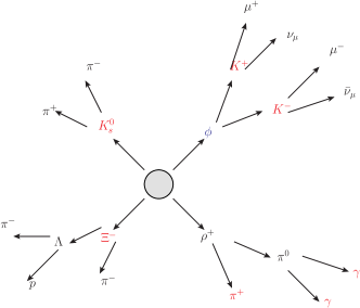
The full event record of the Monte–Carlo event generator cannot be compared directly to experimental results as these are often corrected to a certain definition of primary particles, illustrated in Figure 3. In the context of the heavy-ion developments, pre-defined Projections have been developed for the primary-particle definitions of various experiments. As an example, the definition by the ALICE experiment ALICE-PUBLIC-2017-005 has been implemented in the projection ALICE::PrimaryParticles, where a particle is considered primary if it:

1. has a proper lifetime of $\tau\geq 1\,\mathrm{cm}/c$, and

2. is either produced directly in the interaction;

3. or through the decay of a particle with mean proper lifetime $\tau<1\,\mathrm{cm}/c$.

This provides a reusable selection of primary particles for the analysis of a given experiment. In addition, this approach allows one to clearly identify cases where a requirement has been relaxed for a specific analysis. For example, in Ref. Acharya:2018orn , the $\phi$ as well as its kaon decay daughters have been considered primary.

Figure 3: Visualization of the experimental primary particle definition by Alice ALICE-PUBLIC-2017-005 , with primary particles in red, particles not considered primary in black and resonances which can possibly be added in addition to primary particles in blue.

II.4 Support for multiple runs through reentrant finalize

In order to produce statistically significant results with Rivet analyses, it is often desirable to parallelize the Monte–Carlo generation step over multiple computational units, and merge the individual results into a whole. If the final result includes anything but simple objects such as distributions represented as histograms or mean values, a simple merging will not yield the correct result if the finalize method (see Section II.1) has already been executed. Furthermore, a large number of heavy-ion analyses requires a cross-system merging, to construct, for example, the nuclear-modification factors (see Section IV), which are ratios of distributions obtained in AA to the same distribution in pp, scaled by an appropriate factor.

For this version of Rivet, both of these requirements have been addressed. This solution is called re-entrant finalize, and is implemented in the script rivet-merge. The procedure for re-entrant finalization is as follows:

1. Before finalize, all output objects are saved in raw (un-normalized) form.

2. Finalize is run as always, and both finalized and raw objects are saved in the normal output. Note that raw objects are written before finalize is executed, and any modifications done in finalize will thus not affect the raw objects.

3. By running rivet-merge on one or more produced output files, all used analyses are loaded and all raw objects will be initialized with summed content of all runs to be merged, and finalize will be run again.

For this procedure to work, it is important that all information needed for finalizing the analysis is properly booked in the analysis setup. This implies that only Yoda objects booked in the analysis init method can be used in the analysis’ finalize, thus excluding plain C++ member objects (e.g., int or std::string) as these cannot be made persistent by the framework.

It is worth mentioning that rivet-merge can be run in two different modes. If the files to be merged contain different processes (e.g. one with pp events and another one with AA events for an ${R_{AA}}$ analysis) the program is run in default mode. If, on the other hand, the files contain the result from several identical runs, the weight handling is different and the flag -e or ----equiv should be given to indicate this.

II.5 Analysis options

Normally, the implementation of a Rivet analysis is done such that the user is left with no possibility to influence or modify analysis logic. In some cases, for example when selecting centrality (see Section III.1), this dogma would severely restrict the usability of the framework: A specific combination of analysis and Monte–Carlo event generator may require a user to inform the analysis about the nature of the generated events. For that purpose, the possibility to implement analysis options has been implemented. The value of an analysis option is specified for each individual analysis at run-time, and is then used throughout the analysis pass. Analysis options can have any type that can be constructed from a string.

In practice, the options are given as one or more suffixes to the analysis name, as in

rivet -a $\left\langle\text{analysis name}\right\rangle$:$\left\langle\text{option 1}\right\rangle$=$\left\langle\text{value 1}\right\rangle$:$\left\langle\text{option 2}\right\rangle$=$\left\langle\text{value 2}\right\rangle$

and the corresponding values for a given option is then available in the analysis class by calling the std::string getOption(std::string) function. It is possible to load the same analysis several times, with different option values, and each instance will then be executed with the corresponding optional values. If analysis options are given to an analysis, the output histogram title(s) will be postfixed with a string [Opt=Val] to allow the user to distinguish between histograms generated with different settings.

II.6 Event mixing

The technique of event mixing is often used when studying correlations of two (or more) particles. By mixing data from distinct events, one can correct for acceptance and efficiency effects in a data-driven fashion. Data which is compared by Rivet should already be efficiency corrected. However, the effect of limited acceptance on observables needs to be estimated and is dependent on the distributions of particles and therefore on the Monte–Carlo generator used. A simple example is a rectangular acceptance cut (e.g. $|\eta|<1$). Sampling two particles from a uniform distribution in this region and calculating their pseudorapidity difference, leads to a triangular shape, which has no relation to the underlying physics. While this particular case can be analytically calculated, the distribution has a non-trivial shape as soon as particle production as a function of $\eta$ is not uniform. Nature, and all state-of-the-art MC generators, falls into the latter category.

The implementation of event mixing in Rivet is based on the usual strategy at Lhc experiments CMS:2012qk . In this approach the studied observable is not only built from pairs of particles from a given event, but also from pairs where the particles are from different events. In these mixed events all physical correlations are presumably not present while those originating from the detector effects remain and are thus estimated in a data-driven way.

One way to illustrate event-mixing analyses is to consider some $n$-particle correlation measurement $\Delta$

$$\Delta(E)=\text{Correlation of $n$ particles in $E$}\quad.$$ (1)

The signal is then defined as the event-averaged measurement

$$S=\langle\Delta(E_{i})\rangle_{E}\quad,$$ (2)

while the background is defined as the average over mixed events

$$B=\langle\Delta(E_{i}\cap E_{j})\rangle_{E}\quad,$$ (3)

where $E_{i}\cap E_{j}$ is the random mixture of events $E_{i}$ and $E_{j}$. In the final result

$$R=\frac{S}{B}\quad,$$ (4)

the random correlations are factored out.

The Rivet implementation allows for booking a projection which supplies the mixed event sample, by storing events in memory. The mixed event sample can be divided into bins based on any event property such that the mixed event sample is taken from events which are similar to the signal event in question. Common use cases are centrality and multiplicity, but it is possible to use other properties, for example event shapes (such as eg. transverse spherocity), should the need be.

Finally the possibility that the Monte–Carlo event generator supplies weighted events is considered. If a sample contains weighted events, the particle content of the mixed sample will be weighted as well, with particles being selected to the mixed sample with a probability given by $w_{e}/\sum_{i}w_{i}$, where $w_{e}$ is the weight of the event containing the signal, and $w_{i}$ are the weights off all events in the ensemble of events that form the mixed event.

III Specialized features for heavy-ion collisions

Heavy-ion analyses commonly make use of concepts often not considered relevant for high energy particle physics and, thus, has been not available in Rivet. In this section two new features motivated by physics requirements are outlined. In Section III.1 the framework for centrality is described, and in Section III.2 the generic framework for flow measurements is briefly introduced, and the implementation outlined.

III.1 Centrality framework

The impact parameter ($b$) is the distance between the centers of the colliding nuclei. Its value determines on average the size and the transverse shape of the interaction region of a heavy-ion collision. Observables’ dependence on the geometry of the interaction region, provides insight into the effect of the size and geometry on the underlying physical mechanisms.

Experimentally, centrality classifies collisions on the basis of some measurement (or measurements) which is assumed to depend monotonically on the impact parameter $b$ of a given collision. For a single measurement $X$ which is assumed large for small $b$ and small for large $b$, we can define

$$c_{\mathrm{exp}}=\frac{1}{\sigma_{\mathrm{vis}}}\int_{X}^{\infty}\mathrm{d}X\,\frac{\mathrm{d}\sigma_{\mathrm{vis}}}{\mathrm{dX^{\prime}}}=\frac{1}{N}\int_{X}^{\infty}\mathrm{d}X^{\prime}\frac{\mathrm{d}N}{\mathrm{d}X^{\prime}}\quad,$$ (5)

where $\mathrm{d}\sigma_{\mathrm{vis}}/\mathrm{d}X$ is the full measured distribution of $X$ over the visible cross-section $\sigma_{\mathrm{vis}}$ (typically defined in terms of minimum-bias trigger conditions) of the experiment, and $X$ is the single collision measurement. From a theoretical point of view, the centrality of a single collision can be defined as

$$c_{b}=\frac{1}{\sigma_{\mathrm{inel}}}\int_{0}^{b}\mathrm{d}b^{\prime}\,\frac{\mathrm{d}\sigma_{\mathrm{inel}}}{\mathrm{d}b^{\prime}}\quad.$$ (6)

If $\sigma_{\mathrm{vis}}\approx\sigma_{\mathrm{inel}}$ and $X(b)$ is reasonably well behaved (smooth, positive, monotonically decreasing, with appropriate limiting behaviour) Das:2017ned , $c_{b}\approx c_{\mathrm{exp}}$.

Different experiments use different observables for $X$. In Rivet, several experimental definitions are available, corresponding to different definitions listed in the following. The Alice collaboration Abelev:2013qoq uses the integrated signal in the V0 scintillator systems covering $-3.7<\eta<-1.7$ and $2.8<\eta<5.1$. The Star collaboration Abelev:2006cs uses the number of charged tracks in the central pseudorapidity interval spanning $-0.5<\eta<0.5$, while Brahms used the charged-particle multiplicity at mid-rapidity Bearden:2004yx ; Adamczyk:2003sq . The Atlas collaboration ATLAS:2011ah uses transverse energy deposited in the forward calorimeters located at $4.9<|\eta|<3.2$.

In central heavy ion collisions $c_{b}=c_{\mathrm{exp}}$ to good precision Das:2017ned . In peripheral collisions, or in pA and pp collisions the correspondence is less obvious Bierlich:2018xfw . Moreover, biases introduced by experimental trigger conditions for measurements of $X$, are by construction not included in equation (6). When possible, it should therefore always be preferred to use equation (5) (with appropriate trigger conditions) for estimation of centrality in a simulated event, essentially comparing experimentally obtained $X$ directly to $X$ obtained in a Monte–Carlo. By construction, such an approach also includes biases not related to the detector used, but to the definition of $X$ Adam:2014qja .

Figure 4: Comparison of generated centrality measure generated by Herwig+Pista, Epos-lhc and Pythia 8.2/Angantyr to V0M Amplititude from ALICE. To the left a direct comparison, and to the right a rescaled one (see text).

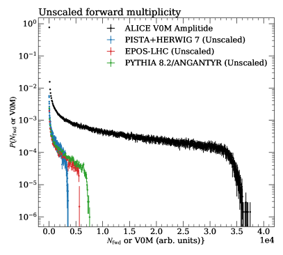
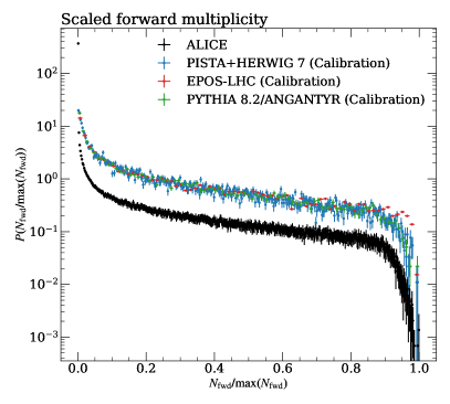
In some cases, neither using equation (6) nor equation (5), is an option. For example, the event generator Jewel Zapp:2013vla does not calculate the underlying event, but considers only a jet quenched in a medium at a certain impact parameter. Other generators, for example Herwig+Pista Bellm:2018sjt ; Bellm:2015jjp attempt to generate the forward-going particle multiplicity but do not obtain good agreement with experimental results. In other cases still, it is not possible to compare to the experimentally measured $X$ without taking into account the detector response. This is for example the case for Alice, where $X$ is defined as a detector response (affected by secondary particles), not unfolded to particle level. This latter case is illustrated in Figure 4, where three soft inclusive approaches (Herwig+Pista, Epos-lhc and Pythia 8.2/Angantyr) are shown together with centrality data from ALICE. In Figure 4 (left) the raw detector response is overlaid with the centrality measure implemented in Rivet, and in Figure 4 (right), a rescaled, normalized version of the centrality measure is shown, comparing to the three MCs. It is clear that direct comparison of MC to experimentally obtained measure (as in Figure 4 (left)) has no physical meaning at all, since the scale of the compared quantities are different, and in order to refrain from potential errors, this should be avoided in analyses. In such cases, a better choice is to use equation 5 on Monte–Carlo and compare the extracted $c_{\mathrm{exp}}$. Note, however, that it is important then to implement the appropriate criteria for $\sigma_{\mathrm{vis}}$ in an equivalent fashion to the experiment compared to. The large excess of experimental measurements at low $X$ are due to contamination from electromagnetic interactions. However, as the analyses often ignore this region, it is less of a problem in direct comparisons to Monte–Carlo results. Remnant contributions from such electromagnetic interactions in more central events, are accounted for by appropriate systematic uncertainties on the experimental results.

In consequence, the slicing from data cannot be naively applied to Monte–Carlo, making the calibration step necessary. In total, four possibilities for centrality estimation can be used:

1. Direct comparison to, and binning in, measured $X$. This, to some extend, circumvents the notion of centrality altogether, but requires that the simulated and measured $X$ are roughly equally distributed. In Rivet, this is selected by the analysis option cent=REF.

2. Comparison to a user-implemented $X$, which should be a particle level, final state observable to get generator calibrated centrality. As noted above, it is important to impose the same requirements as used by the experiment to determine $\sigma_{\mathrm{vis}}$. In Rivet, this is selected by the analysis option cent=GEN.

3. Centrality binning of Monte–Carlo according to equation (6) — $b$ centrality. In Rivet, this is selected by the analysis option cent=IMP.

4. Provide a centrality percentile number in the HepMC heavy-ion record (available from HepMC 3.0). In Rivet, this is selected by the analysis option cent=RAW.

Possibilities 2 and 3 require the user to perform a calibration run, to generate the distribution of either $X$ or $b$ and then evaluate the integrals in equations (6) or (5). The result of the calibration pass can then be used in subsequent passes with the analysis calculating the desired centrality-dependent observable. Concrete examples of how to perform such tasks using Rivet, are given in Section IV.

III.2 Flow measurements

In heavy-ion collisions, the study of azimuthal anisotropy of particle production is used to understand the transport properties of the produced medium, as well as the geometry of the initial state Ollitrault:1992bk . This is quantified in flow coefficients $v_{n}$’s, obtained by a Fourier expansion of the particle yield with respect to the reaction plane $\Psi_{n}$

$$E\frac{\mathrm{d}^{3}N}{\mathrm{d}^{3}p}=\frac{1}{2\pi}\frac{\mathrm{d}^{2}N}{{p_{\mathrm{T}}}\mathrm{d}{p_{\mathrm{T}}}\mathrm{d}y}\left(1+2\sum_{n=1}^{\infty}v_{n}\cos([n(\phi-\Psi_{n})])\right)\quad,$$ (7)

where $E$ is the energy of the particle, ${p_{\mathrm{T}}}$ is the transverse momentum, $\phi$ is the azimuthal angle and $y$ is the rapidity. As indicated, the coefficients are in general dependent on $y$ and ${p_{\mathrm{T}}}$. The present Rivet implementation allows one to perform a simple calculation of coefficients differentially with respect to ${p_{\mathrm{T}}}$, as well as integrated coefficents.

Since the reaction plane cannot be determined experimentally, flow coefficients are estimated from two- or multi-particle correlations. For example, using two-particle correlations:

$$\langle v^{2}_{n}\rangle\approx\langle\cos(n(\phi_{1}-\phi_{2})))\rangle=\langle\exp(in(\phi_{1}-\phi_{2}))\rangle\quad,$$ (8)

where $\phi_{1}=\phi_{2}$ is excluded from the average. A more advanced technique – with several benefits, which are introduced in the following – calculates multi-particle cumulants from $Q$-vectors Bilandzic:2010jr ($Q_{n}=\sum_{k=1}^{M}w_{k}\exp(in\phi_{k})$ for an event with $M$ particles), which are combined into $m$-particle correlators denoted $\langle m\rangle_{n_{1},n_{2},...,n_{m}}$. Expressing $m$-particle correlators in terms of $Q$-vectors follows the Generic Framework Bilandzic:2013kga , where the formula for any $m$-particle correlator is written as:

$$\langle m\rangle_{n_{1},n_{2},...n_{m}} =\frac{N\langle m\rangle_{n_{1},n_{2},\ldots,n_{m}}}{N\langle m\rangle_{0,0,\ldots,0}}\quad\text{with}$$ (9)

$$N\langle m\rangle_{n_{1},n_{2},\ldots,n_{m}} =\sum_{\begin{subarray}{c}k_{1},k_{2},\ldots,k_{m}=1\\ k_{1}\neq k_{2}\neq\ldots k_{m}\end{subarray}}^{M}\exp(i(n_{1}\phi_{k_{1}}+n_{2}\phi_{k_{2}}+\cdots+n_{m}\phi_{k_{m}}))\quad.$$ (10)

This expression allows one to easily calculate any correlator, since $N\langle m\rangle_{n_{1},n_{2},...,n_{m}}$ can be calculated from $Q$-vectors, with the concrete expressions obtained using a recursion relation Bilandzic:2013kga , for any values of $m$ and $n_{i}$. As an example, for $m=2$, one obtains:

$$N\langle 2\rangle_{n_{1},n_{2}}=Q_{n_{1}}Q_{n_{2}}-Q_{n_{1}+n_{2}}\quad.$$ (11)

For the special case of $n_{1}=n_{2}=n$, the two-particle correlator directly becomes:

$$\langle 2\rangle_{n}=\frac{|Q_{n}|^{2}-M}{M(M-1)}\quad.$$ (12)

Evaluation of the product in the numerator $|Q_{n}|^{2}=\sum_{k,l}\exp(in(\phi_{k}-\phi_{l}))$ reveals that the correlator reduces to equation (8). However, when evaluating using $Q$-vectors, the process requires only a single pass over data, as opposed to nested passes. Without the use of $Q$-vectors, the complexity of an $m$-particle correlator is obviously $O\left(M^{m}\right)$ while the above approach is at most $O\left(M\log M\right)$. In a heavy-ion event where $M$ can be 10 000 tracks, this is absolutely crucial. From the correlators, a large number of flow observables can be defined. In most analyses, cumulants $c_{n}\{m\}$ (where curly braces represent the order of the $m$-particle correlation) are calculated from correlators with $n_{1}=n_{2}=...=n_{m}=n$. The most common use cases are implemented along with uncertainty estimation (see below):

$$c_{n}\{2\}= \langle\langle 2\rangle\rangle_{n,-n}$$

$$c_{n}\{4\}= \langle\langle 4\rangle\rangle_{n,n,-n,-n}-2\langle\langle 2\rangle\rangle^{2}_{n,-n}$$

$$c_{n}\{6\}= \langle\langle 6\rangle\rangle_{n,n,n,-n,-n,-n}-9\langle\langle 2\rangle\rangle_{n,-n}\langle\langle 4\rangle\rangle_{n,n,-n,-n}+12\langle\langle 2\rangle\rangle^{3}_{n,-n}$$

$$c_{n}\{8\}= \langle\langle 8\rangle\rangle_{n,n,n,n,-n,-n,-n}-16\langle\langle 6\rangle\rangle_{n,n,n,-n,-n,-n}\langle\langle 2\rangle\rangle_{n,-n}-18\langle\langle 4\rangle\rangle^{2}_{n,n,-n,-n}$$

$${}+144\langle\langle 4\rangle\rangle_{n,n,-n,-n}\langle\langle 2\rangle\rangle^{2}_{n,-n}-144\langle\langle 2\rangle\rangle^{4}_{n,-n}\quad.$$ (13)

The double averages denote an all-event average of event averages. Even higher-order cumulants, or other combinations of correlators, such as Symmetric Cumulants ALICE:2016kpq can be easily added by the user, as the framework allows the user to fully access the correlators. The cumulants are finally transformed into flow coefficients

$$v_{n}\{m\}=\left(k_{m/2}c_{n}\{m\}\right)^{\frac{1}{m}}\quad,$$ (14)

where the coefficient $k_{m}$ is written here for convenience for $m<4$:

$$k_{m}=\left\{1,-1,\frac{1}{4},-\frac{1}{33}\right\}\quad.$$ (15)

Differential flow observables are constructed using an additional correlator, limited to a certain phase space. In the case of the implementation in Rivet, this is restricted to observables differential in ${p_{\mathrm{T}}}$. The differential correlator can be constructed in a similar fashion Bilandzic:2013kga as the integrated ones in equation (9), but the transformation to differential flow coefficients differs. Denoting the differential $m$-particle correlator $\langle m^{\prime}\rangle$, the differential two-particle cumulant and the corresponding differential flow coefficient are given by:

$$d_{n}\{2\}=\langle\langle 2^{\prime}\rangle\rangle\quad\text{and}\quad v^{\prime}_{n}\{2\}=\frac{d_{n}\{2\}}{\sqrt{c_{n}\{2\}}}\quad,$$ (16)

where $c_{n}\{2\}$ is a reference cumulant calculated for the full phase space as above. In the same way, the differential four-particle cumulant and the corresponding differential flow coeffiecient are:

$$d_{n}\{4\}=\langle\langle 4^{\prime}\rangle\rangle-2\langle\langle 2\rangle\rangle\langle\langle 2^{\prime}\rangle\rangle\quad\text{and}\quad v^{\prime}_{n}\{4\}=-\frac{d_{n}\{4\}}{(-c_{n}\{4\})^{3/4}}\quad.$$ (17)

The statistical uncertainty on cumulants and flow coefficients is calculated by a simple variance method, often denoted as bootstrap LWasserman method in experimental literature. Instead of propagating the sampling uncertainty on the individual correlators through the (long) expressions for cumulants and flow coefficients, the calculation is internally split up into sub-samples. The default behaviour is to display the square root of the sample variance as statistical uncertainty, but the user can choose to use the envelope instead.

III.2.1 Suppressing non-flow with an $\eta$-gap

The approximate equality in equation (8) becomes a full equality in the absence of non-flow effects, which are correlations arising from other sources than typically attributed to collective expansion Voloshin:2008dg . Non-flow effects can arise from several sources, such as jet production or resonance decay, and are few-particle correlations as opposed to flow which is correlation of all particles to a common symmetry plane. The idea behind the $\eta$-gap or sub-event method is to suppress sources of non-flow which are local in (pseudo)rapidity. The non-flow is then suppressed by requiring that particle measurements contributing to a correlator must come from different parts of the detector acceptance, usually separated in pseudorapidity. Using equation (8), an $\eta$-gap can be implemented simply by requiring that the two particles come from two different sub-events, here labeled $A$ and $B$:

$$\langle v^{2}_{n}\rangle\approx\langle\exp(in(\phi^{A}_{1}-\phi^{B}_{2}))\rangle\quad.$$ (18)

Translating to $Q$-vectors, it is first noted that $\phi_{1}=\phi_{2}$ does not need to be excluded from the average in this case, as it is excluded by construction. Equation (11) reduces to $N\langle 2\rangle_{n_{1},n_{2}}=Q^{A}_{n_{1}}Q^{A}_{n_{2}}$, where superscripts $A$ and $B$ indicates that $Q$-vectors are calculated in that specific sub-event only, as $Q^{X}_{n}=\sum^{M_{X}}_{k=1}\exp(in\phi^{X}_{k})$. This procedure is generalized to multi-particle correlations, by removing terms from the correlator where cross-terms do not share a common sub-event.

In Rivet, correlators with two sub-events are implemented, with the possibility of calculating both integrated and differential flow.

Figure 5: Centrality observables from the analyses BRAHMS_2004_AUAUCentrality with Pythia 8.2/Angantyr model Bierlich:2018xfw displaying the generated calibration curve (left) and the impact parameter calibration curve (right).

IV Examples of implemented heavy-ion analyses

In this section, some of the implemented Rivet analyses using new features are presented, along with detailed instructions for a user to run the analyses and plot the resulting figures.

The centrality framework introduced in Section III.1 is used by many analyses, each one implementing the centrality estimator of the respective experiment. In these cases the analysis implementation relies on an analysis for centrality calibration, called e.g., ALICE_2015_PBPBCentrality, BRAHMS_2004_AUAUCentrality, and STAR_BES_CALIB. These can be reused by many analyses sharing the same centrality estimator.

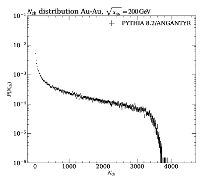
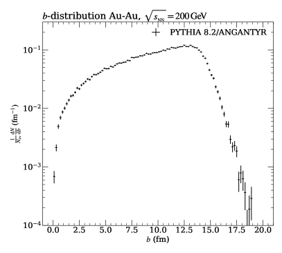
Executing the centrality calibration analysis fills histograms for each defined centrality estimator, for example the impact parameter and the number of charged particles or their energy in the rapidity region where the relevant detector is situated. Figure 5 exemplifies the calibration for Brahms, for which an unfolded measure does not exist, and the options 2 or 3 (GEN and IMP) must be used.

In order to use the generated calibration histograms in the actual analyses, they must be pre-loaded when running the analysis code. The analysis will then calculate the percentile of the calibration curve for the value determined in the newly generated event and, thus, allow the user to retrieve the centrality for the current event.

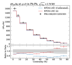
Figure 6 presents results from Brahms, Star and Alice, using separate centrality calibrations. Comparison to Pythia 8.2/Angantyr and Epos-lhc is performed. In the considered analysis by Brahms (BRAHMS_2004_I647076 Bearden:2004yx ), only the $0-5\%$ centrality bin is used, meaning that all other events are vetoed by the analysis code. The centrality definition is selected at runtime using, in this case, either the analysis option (see Section II.5) GEN (for generator calibrated) or IMP (for impact parameter). In the Star analysis STAR_2017_I1510593 Adamczyk:2017iwn , several centrality bins are analysed. The Alice analysis ALICE_2010_I880049 Aamodt:2010cz calibrates using the centrality analyses presented in Section III.1 (cf. Figure 4).

Figure 6: Results from the analyses BRAHMS_2004_I647076 (left; invariant ${p_{\mathrm{T}}}$ of $\pi^{-}$ in $0<y<0.1$), STAR_2017_I151059 (middle; invariant ${p_{\mathrm{T}}}$ for $K^{+}$ in $|y|<0.1$) and ALICE_2010_I880049 (right; $\mathrm{d}N_{\mathrm{ch}}/\mathrm{d}\eta$ vs. centrality) utilizing centrality calibration.

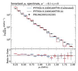
To reproduce those results based on a HepMC file containing AA collisions generated by the considered generators, the following steps need to be followed for the example of the Brahms analysis:

1. Run the calibration analysis

   rivet events.hepmc -a BRAHMS_2004_AUAUCentrality -o calibration.yoda
   

2. Plot the calibration results from Figure 5

   rivet-mkhtml calibration.yoda
   

3. Run the analysis with the calibration file pre-loaded, for both centrality selections:

   rivet events.hepmc -p calibration.yoda  \
         -a BRAHMS_2004_I647076:cent=IMP \
         -a BRAHMS_2004_I647076:cent=GEN -o result
   

4. Plot the analysis result from Figure 6

   rivet-mkhtml result.yoda
   

Note that in this case (and in fact in all currently implemented heavy ion analyses), the calibration and analysis steps are carried out on the same event sample. This would not be the case for a signal analysis considering a signal process (eg. $Z$-production). Here the calibration step would be carried out on a minimum bias sample, and the signal step on a signal sample.

The real power of Rivet analyses is, however, not to compare a single generator at a time, but the ability to compare several generators to the same experimental data at once. This use case is shown in Figure 6 (middle), where both Epos-lhc and Pythia 8.2/Angantyr are compared to Au–Au data at ${{\sqrt{s_{\scriptscriptstyle\mathrm{NN}}}}=27.6\,\mathrm{{\mathrm{Ge\kern-0.70007ptV}}}}$ obtained by Star Adamczyk:2017iwn . In this case, the calibration must be run for both generators, as the output will in general be different. The shown figure can thus be obtained by slightly extending the workflow outlined above:

rivet epos-events.hepmc -a STAR_BES_CALIB -o epos-calib
rivet pythia-events.hepmc -a STAR_BES_CALIB -o pythia-calib
rivet epos-events.hepmc -p epos-calib.yoda -a STAR_2017_I1510593 \
  -o epos-result
rivet pythia-events.hepmc -p pythia-calib.yoda -a STAR_2017_I1510593 \
  -o pythia-result
rivet-mkhtml epos-result.yoda pythia-result.yoda

Note from the last line that comparison plots can be produced directly by the rivet-mkhtml script. Such comparisons are performed using large scale volountary computing resources as part of the MCplots project Karneyeu:2013aha . MCplots is currently being updated and extented to include heavy-ion results and Monte–Carlo by members of the ALICE collaboration.

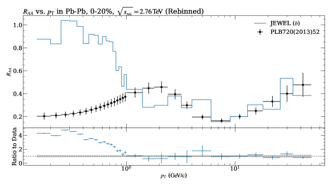
The feature reentrant finalize introduced in Section II.4, is for example used in the analysis ALICE_2012_I1127497. The main observable is the nuclear-modification factor ${R_{AA}}$ defined as the ratio of the yield in AA collisions over pp collisions scaled by an appropriate factor $N_{\mathrm{coll}}$ to accommodate for the trivial scaling of binary collisions Miller:2007ri :

$${R_{AA}}=\frac{\left.\mathrm{d}^{2}N_{\mathrm{ch}}/\mathrm{d}{p_{\mathrm{T}}}\mathrm{d}y\right|_{AA}}{N_{\mathrm{coll}}\left.\mathrm{d}^{2}N_{\mathrm{ch}}/\mathrm{d}{p_{\mathrm{T}}}\mathrm{d}y\right|_{pp}}$$ (19)

In order to compute this quantity, Rivet is executed three times, first for a generator with AA settings, second with pp settings, and a third and final time to compute the ratio. A comparison of this observable to a calculation with the Jewel generator is shown in Figure 7, and can be performed with the following steps, given generated HepMC files of pp and AA events by Jewel.

Figure 7: Nuclear-modification factor ${R_{AA}}$ measured by ALICE Abelev:2012hxa compared to Jewel model calculations. The region below $1\,{{\mathrm{Ge\kern-0.70007ptV}}\kern-1.99997pt/\kern-0.50003pt\mathrm{c}}$ is not attempted to be modelled correctly in Jewel resulting in the large discrepancy. Note, that data and MC have been rebinned to allow a reasonable comparison.

1. The desired centrality range is set when events are generated in Jewel. The centrality value as well as the impact parameter are saved in the HepMC output. The usage of the raw centrality values is supported only from HepMC 3.0 onwards (see Section III.1), therefore the impact parameter centrality calibration is needed to be applied after events have been generated in the full centrality interval (0–100%):

   rivet aa-sample.hepmc --ignore-beams -a ALICE_2015_PBPBCentrality
       -o calibration.yoda
   

2. The Rivet analysis is run on the pp sample:

   rivet pp-sample.hepmc --ignore-beams -a ALICE_2012_I1127497
       -o jewel-pp.yoda
   

3. Next the Rivet analysis is run on the AA sample. Note the beam option signifying that this is an AA run. Since the Jewel event generator does not supply this information in the HepMC file, but denotes all beams as pp beams, the analysis requires this additional information:

   rivet aa-sample.hepmc --ignore-beams -p calibration.yoda
       -a ALICE_2012_I1127497:beam=HI:cent=IMP -o jewel-aa.yoda
   

4. The two samples must be merged, and the ratio plots constructed, with rivet-merge, which loads histograms from the two runs above, and runs finalize on the preloaded histograms:

   rivet-merge --merge-option beam --merge-option cent
       jewel-pp.yoda jewel-aa.yoda -o jewel-merged.yoda
   

   The optional argument merge-option removes the analysis options beam and cent from the heavy ion sample.

5. The merged sample can be plotted. There is no need to plot the unmerged histograms, as all histograms are contained in the merged file.

   rivet-mkhtml jewel-merged.yoda
   

V Understanding biases in simulation and data

Apart from direct validation of a given Monte–Carlo event generator, the analysis capabilities of Rivet are useful as tools to reveal inherent biases in representation of data. In this section the use of the physics motivated extensions presented in Section III are exemplified by presenting short analyses of centrality biases introduced by using different centrality observables for theory and data (Section V.1) and from inclusion of non-flow effects in flow measurements (Section V.2). These two effects are well known, and chosen to show the capabilities of the framework, rather than presenting an independent physics point.

V.1 Centrality observables

In pA collisions, such as those performed at the Lhc with p–Pb collisions at ${{\sqrt{s_{\scriptscriptstyle\mathrm{NN}}}}=5.02\,\mathrm{{\mathrm{T\kern-0.50003pte\kern-0.70007ptV}}{}}}$, and recorded by the Atlas experiment Aad:2015zza , the notion of centrality is used as in AA collisions, shown in Section IV, but without the clear relation to the physical impact parameter. Since the physical impact parameter is well defined and useful from a theoretical point of view (as it can be used to infer properties of a created QGP phase), the correlation between modelled impact parameter and measured centrality is worth having direct access to, as the effects of possible differences between the two in a measurement is important to understand.

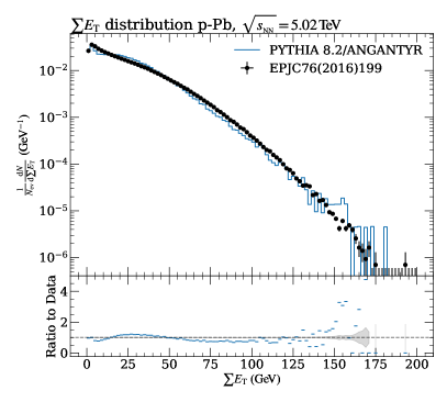
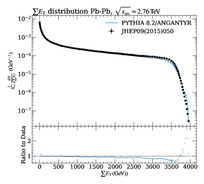
The Rivet centrality implementation offers the possibility to study such effects directly in specific simulations, by comparing results from measured centrality to Monte–Carlo using different centrality definitions. Consider the centrality measure used by Atlas, shown in Figure 8, which is the $\sum{E_{\mathrm{T}}}$ in the forward (lead) going direction Aad:2015zza , overlaid with a comparison to Pythia 8.2/Angantyr. This can be contrasted with the similar centrality measure used by Atlas in Pb–Pb collisions at ${{\sqrt{s_{\scriptscriptstyle\mathrm{NN}}}}=2.76\,\mathrm{{\mathrm{T\kern-0.50003pte\kern-0.70007ptV}}{}}}$ Aad:2015wga , which is $\sum{E_{\mathrm{T}}}$ in both forward and backward directions. For both centrality measures, it should be noted that data points are read-off from the paper. Furthermore the distributions are not unfolded. This adds an unknown source of uncertainty to the direct comparison to the centrality, as well as to all derived results, when the experimental centrality estimate is used.

Figure 8: Centrality measure by Atlas for p–Pb at ${{\sqrt{s_{\scriptscriptstyle\mathrm{NN}}}}=5.02\,\mathrm{{\mathrm{T\kern-0.50003pte\kern-0.70007ptV}}{}}}$ Aad:2015zza (left) and Pb–Pb at ${{\sqrt{s_{\scriptscriptstyle\mathrm{NN}}}}=2.76\,\mathrm{{\mathrm{T\kern-0.50003pte\kern-0.70007ptV}}{}}}$ Aad:2015wga (right), compared to Pythia 8.2. Note that data points are not unfolded, and taken from the figures in the paper.

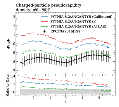
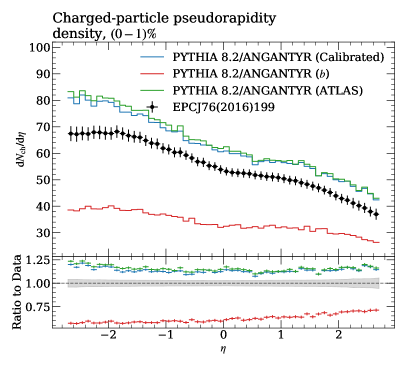
In Figure 9, the $\mathrm{d}N_{\mathrm{ch}}/\mathrm{d}\eta$ distributions for the three different centrality selections, experimental reference calibration (Experiment, option REF), generator calibrated (Calibrated, option GEN), and impact parameter ($b$, option IMP) in p–Pb are shown for peripheral (60-90%) (left) and central (0-1%) (right) events Aad:2015zza . We see a small, but systematic, overestimate of the charged-particle pseudorapidity density when using either generator or experimentally calibrated centrality estimators. The impact parameter based centrality estimator has overall larger deviations from experimental results (also in centrality classes not shown here, see ref. Bierlich:2018xfw for more comparisons), but without any clear systematics in the deviations.

Figure 9: Charged-particle pseudorapidity density as a function of pseudorapidity in p–Pb at ${{\sqrt{s_{\scriptscriptstyle\mathrm{NN}}}}=5.02\,\mathrm{{\mathrm{T\kern-0.50003pte\kern-0.70007ptV}}{}}}$ for peripheral (60-90%) (left) and central (0-1%) (right) events Aad:2015wga , compared to Pythia 8.2.

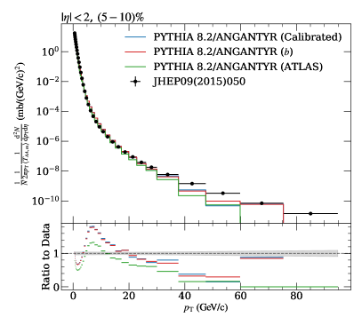
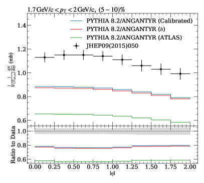
In Figure 10 the charged-particle multiplicity in Pb–Pb differential in ${p_{\mathrm{T}}}$ (left) and $\eta$ for $1.7\,{{\mathrm{Ge\kern-0.70007ptV}}\kern-1.99997pt/\kern-0.50003pt\mathrm{c}}<{p_{\mathrm{T}}}<2.0\,{{\mathrm{Ge\kern-0.70007ptV}}\kern-1.99997pt/\kern-0.50003pt\mathrm{c}}$ (right) in the 5-10% centrality bin are shown Aad:2015wga , again for the three different centrality estimators. Here, the results from the generated and impact parameter centrality estimators fully coincides, thus in agreement with the assumption that the measured centrality (equation (5)) coincides with theoretical centrality (equation (6)) in AA collisions. It is also seen that comparison using the measured experimental centrality measure, deviates from the two others, as expected.

Figure 10: Charged-particle multiplicity as function of ${p_{\mathrm{T}}}$ (left) and $\eta$ for $1.7\,{{\mathrm{Ge\kern-0.70007ptV}}\kern-1.99997pt/\kern-0.50003pt\mathrm{c}}{}<{p_{\mathrm{T}}}<2.0\,{{\mathrm{Ge\kern-0.70007ptV}}\kern-1.99997pt/\kern-0.50003pt\mathrm{c}}$ (right) in Pb–Pb at ${{\sqrt{s_{\scriptscriptstyle\mathrm{NN}}}}=2.76\,\mathrm{{\mathrm{T\kern-0.50003pte\kern-0.70007ptV}}{}}}$, in the 5-10% centrality bin Aad:2015wga , compared to Pythia 8.2.

V.2 Non-flow effects

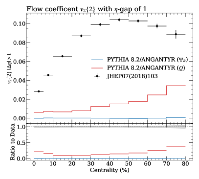
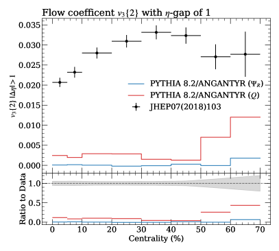
The $v_{2}$ and $v_{3}$ measured by Alice in Pb–Pb collisions, at ${{\sqrt{s_{\scriptscriptstyle\mathrm{NN}}}}=2.76\,\mathrm{{\mathrm{T\kern-0.50003pte\kern-0.70007ptV}}{}}}$ as a function of centrality, is shown in Figure 11 together with comparisons to Pythia 8.2/Angantyr simulations Acharya:2018lmh . The simulations were obtained using two different approaches. First the event plane method, where equation (7) is evaluated directly, giving $\langle v_{n}\rangle=\langle\cos\left(n\left(\phi-\Psi\right)\right)\rangle$. The used value for the event plane angle $\Psi$ can be evaluated in simulations, but not in data. Secondly the Generic Framework (GF) implementation in Rivet, described in Section III.2, is used to estimate $v_{2}$ and $v_{3}$ with two-particle correlations as it is done in the experiment. In the former case, the Pythia 8.2 simulations are consistent with 0. This is expected, as the typical mechanisms associated with the non-flow (jets, resonance decays) are not correlated with the event plane, and thus any coincidental correlations are averaged out. On the other hand, this is not true for the simplest case of two-particle correlations. In particular, back-to-back jets give rise to strong correlations that are unrelated to the hydrodynamical evolution of the system. As a result, Pythia 8.2 predicts non-zero $v_{2}$ and $v_{3}$ values calculated with two-particle correlations, as seen in Figure 11. We note that the non-flow effects are more pronounced for $v_{2}$ and increase for peripheral Pb–Pb collisions, where the $\mathrm{d}N_{\mathrm{ch}}/\mathrm{d}\eta$ is lower and therefore the different non-flow sources get less averaged out. It is noted that the non-flow contribution is here shown to be sizeable for $v_{2}\{2\}$ even with a required minimum separation in $\eta$ between the two correlated particles.

Figure 11: Flow coefficients $v_{2}\{2\}$ (left) and $v_{3}\{2\}$ (right) in Pb–Pb collisions, at ${{\sqrt{s_{\scriptscriptstyle\mathrm{NN}}}}=2.76\,\mathrm{{\mathrm{T\kern-0.50003pte\kern-0.70007ptV}}{}}}$ as a function of centrality, evaluated with the event plane method ($\Psi_{R}$) and the Generic Framework ($Q$) implementation in Rivet. Data from Alice Acharya:2018lmh compared to Pythia 8.2.

VI Collective effects in pp collisions

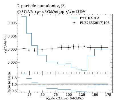
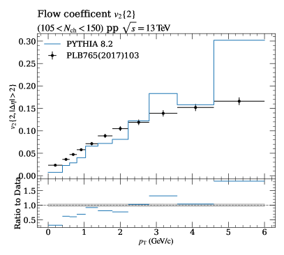
The discovery of heavy-ion-like effects in pp collisions has spurred a lot of interest from the proton-proton Monte–Carlo authors to introduce models for such effects Bierlich:2017vhg ; Gieseke:2017clv ; Duncan:2018gfk ; Gieseke:2018gff ; Bierlich:2015rha ; Bierlich:2014xba ; Christiansen:2015yqa ; Fischer:2016zzs . The inclusion of heavy-ion features in Rivet will aid this development, as such features can be used directly in new analyses for pp as well. As an example, the seminal results from the Cms experiment on two- and multi-particle correlations Khachatryan:2016txc and from the Alice experiment on strangeness enhancement ALICE:2017jyt has been implemented in Rivet analyses CMS_2017_I1471287 and ALICE_2016_I1471838. Results from the former shown in Figure 12.

Figure 12: Example flow observables from pp collisions Khachatryan:2016txc , compared to simulation with Pythia 8.2. Analysis performed with the implementation of the Generic Framework for flow measurements Bilandzic:2013kga presented in Section III.2.

The analysis is implemented with the flow framework presented in Section III.2. In Figure 12 the cumulant $c_{2}\{2\}$ as a function of charged-particle multiplicity (left, equation (III.2)), and the corresponding flow coefficient as a function of transverse momentum (right) are shown.

VII Conclusion and future work

Extensions to the Rivet framework to facilitate comparisons between Monte–Carlo event generators and data have been presented. The Rivet framework is a standard tool for preservation of Lhc analyses of proton–proton collisions, and with the presented extensions, the framework is ready to start taking a similar role for heavy-ion physics.

There are, however, areas where the updated framework is foreseen to be further extended in order to allow for better comparisons to jet physics studies, reproduction of global fits of QGP properties, as well as allowing for comparison of simulation tools developed for heavy-ion physics.

One avenue of further development is jet observables. Rivet includes an interface to the popular FastJet package Cacciari:2011ma for jet reconstruction, which already includes some functionality for sub-jet observables geared towards heavy-ion collisions Andrews:2018jcm . A more substantial problem for preservation of jet analyses is that of handling the large “underlying event” of a heavy-ion collision. A preliminary Rivet implementation to perform background subtraction and QGP back-reactions for specific models is available KunnawalkamElayavalli:2017hxo , but no truly model independent prescription exist. Due to large differences between models, it may even be such that experimental background subtraction cannot be fully reproduced for models unless the model also attempts to describe the full underlying event. In such case a better option might be to publish data without background subtraction for model comparisons.

Another future direction involves expanding the possibility for post-processing beyond what re-entrant finalization allows. Specifically to add the possibility to perform fits used in experimental analyses, such as for example reinterpretation in terms of simple thermal models like Boltzmann–Gibbs Blast Wave for AA Schnedermann:1993ws or Lévy–Tsallis for pp Tsallis:1987eu ; Abelev:2006cs . A technically similar development for high energy physics is realized in the Contur package Butterworth:2016sqg , which constrains BSM physics using Standard Model measurements implemented in Rivet. Reinterpretation of heavy-ion analyses could be performed in a technically similar way, possibly also as an additional software package. Such an extension could also cater to theoretical models not suitable for direct event-by-event analysis.

VIII Acknowledgements

We thank the Discovery Center at the Niels Bohr Institute for hosting a successful workshop in August 2018, consolidating the efforts described in this paper, and in particular the NBI Alice group for providing organizational support. The workshop was further supported by the Marie Skłodowska-Curie Innovative Training Network MCnetITN3 (grant agreement 722104).

The authors would further like to acknowledge support from individual funding bodies:

• CB was supported by the Swedish Research Council, contract number 2017-003.

• AB was supported by The Royal Society via University Research Fellowship grant UF160548.

• COR and LL were supported in part by the European Research Council (ERC) under the European Union’s Horizon 2020 research and innovation program (grant agreement No 668679), and in part by the Swedish Research Council, contract number 2016-05996.

• LL was supported in part by the Swedish Research Council, contract number 2016-03291, and the Knut and Alice Wallenberg foundation, contract no 2017.0036.

• PaKi acknowledges support by the BMBF under grant number 05H18VKCC1.

Appendix A Analyses with heavy ion features

This appendix contains a list of all Rivet analyses implementing one or more heavy ion features, or heavy ion beams, at the time of writing, shown in table 1. It includes a mention of features used, as a handy guide to anyone looking for inspiration to implement a specific feature into their analyses. An up-to-date list of all Rivet analyses can be found at https://rivet.hepforge.org/.

Table 1: All Rivet analyses implementing one or more heavy ion features, or heavy ion beams. An up-to-date list can be found at https://rivet.hepforge.org.

Analysis name System ${\sqrt{s_{\scriptscriptstyle\mathrm{NN}}}}{}$ Heavy ion features Reference ALICE_2010_I880049 Pb–Pb $2.76\,{\mathrm{T\kern-0.50003pte\kern-0.70007ptV}}$ centrality, primary particles, heavy ion container Aamodt:2010cz ALICE_2012_I930312 Pb–Pb $2.76\,{\mathrm{T\kern-0.50003pte\kern-0.70007ptV}}$ centrality, heavy ion container, re-entrant finalize Aamodt:2011vg ALICE_2012_I1127497 Pb–Pb $2.76\,{\mathrm{T\kern-0.50003pte\kern-0.70007ptV}}$ centrality, heavy ion container, re-entrant finalize Abelev:2012hxa ALICE_2012_I1126966 Pb–Pb $2.76\,{\mathrm{T\kern-0.50003pte\kern-0.70007ptV}}$ centrality, primary particles Abelev:2012wca ALICE_2013_I1225979 Pb–Pb $2.76\,{\mathrm{T\kern-0.50003pte\kern-0.70007ptV}}$ centrality, primary particles Abbas:2013bpa ALICE_2014_I1243865 Pb–Pb $2.76\,{\mathrm{T\kern-0.50003pte\kern-0.70007ptV}}$ centrality, primary particles ABELEV:2013zaa ALICE_2014_I1244523 p–Pb $5.02\,{\mathrm{T\kern-0.50003pte\kern-0.70007ptV}}$ centrality, primary particles Abelev:2013haa ALICE_2016_I1394676 Pb–Pb $2.76\,{\mathrm{T\kern-0.50003pte\kern-0.70007ptV}}$ centrality, primary particles Adam:2015kda ALICE_2016_I1419244 Pb–Pb $5.02\,{\mathrm{T\kern-0.50003pte\kern-0.70007ptV}}$ centrality, generic framework Adam:2016izf ALICE_2016_I1507090 Pb–Pb $5.02\,{\mathrm{T\kern-0.50003pte\kern-0.70007ptV}}$ centrality, primary particles Adam:2016ddh ALICE_2016_I1507157 pp $7\,{\mathrm{T\kern-0.50003pte\kern-0.70007ptV}}$ event mixing Adam:2016iwf ATLAS_2015_I1360290 Pb–Pb $2.76\,{\mathrm{T\kern-0.50003pte\kern-0.70007ptV}}$ centrality Aad:2015wga ATLAS_2015_I1386475 p–Pb $5.02\,{\mathrm{T\kern-0.50003pte\kern-0.70007ptV}}$ centrality Aad:2015zza ATLAS_PBPB_CENTRALITY Pb–Pb $2.76\,{\mathrm{T\kern-0.50003pte\kern-0.70007ptV}}$ centrality Aad:2015wga ATLAS_pPb_Calib p–Pb $5.02\,{\mathrm{T\kern-0.50003pte\kern-0.70007ptV}}$ centrality Aad:2015zza BRAHMS_2004_I647076 Au–Au $200\,{\mathrm{Ge\kern-0.70007ptV}}$ centrality, primary particles Bearden:2004yx CMS_2017_I1471287 pp $13\,{\mathrm{T\kern-0.50003pte\kern-0.70007ptV}}$ generic framework Khachatryan:2016txc LHCF_2016_I138587 p–Pb $5.02\,{\mathrm{T\kern-0.50003pte\kern-0.70007ptV}}$ - Adriani:2015iwv STAR_2016_I1414638 Au–Au $7.7-200\,{\mathrm{Ge\kern-0.70007ptV}}$ centrality Adamczyk:2016exq STAR_2017_I1510593 Au–Au $7.7-39\,{\mathrm{Ge\kern-0.70007ptV}}$ centrality Adamczyk:2017iwn

References

- (1) Buckley A, Butterworth J, Lonnblad L, Grellscheid D, Hoeth H, Monk J, Schulz H and Siegert F 2013 Comput. Phys. Commun. 184 2803–2819 (Preprint eprint 1003.0694)
- (2) Schukraft J 2017 Nucl. Phys. A967 1–10 (Preprint eprint 1705.02646)
- (3) Putschke J H et al. 2019 (Preprint eprint 1903.07706)
- (4) Khachatryan V et al. (CMS) 2010 JHEP 09 091 (Preprint eprint 1009.4122)
- (5) Adam J et al. (ALICE) 2017 Nature Phys. 13 535–539 (Preprint eprint 1606.07424)
- (6) Citron Z et al. 2019 Report from Working Group 5 Report on the Physics at the HL-LHC,and Perspectives for the HE-LHC ed Dainese A, Mangano M, Meyer A B, Nisati A, Salam G and Vesterinen M A pp 1159–1410 (Preprint eprint 1812.06772)
- (7) A brief review of the framework, with emphasis on functionality necessary for later sections, is given here. For a full description of the Rivet framework, the reader is referred to the original manual Buckley:2010ar or the manual of Rivet version 3 Bierlich:2019rhm.
- (8) Sjöstrand T, Ask S, Christiansen J R, Corke R, Desai N, Ilten P, Mrenna S, Prestel S, Rasmussen C O and Skands P Z 2015 Comput. Phys. Commun. 191 159–177 (Preprint eprint 1410.3012)
- (9) Bellm J et al. 2016 Eur. Phys. J. C76 196 (Preprint eprint 1512.01178)
- (10) Bíró G, Barnaföldi G G, Papp G, Gyulassy M, Lévai P, Wang X N and Zhang B W 2019 PoS HardProbes2018 045 (Preprint eprint 1901.04220)
- (11) Skands P, Carrazza S and Rojo J 2014 Eur. Phys. J. C74 3024 (Preprint eprint 1404.5630)
- (12) Khachatryan V et al. (CMS) 2016 Eur. Phys. J. C76 155 (Preprint eprint 1512.00815)
- (13) 2012
- (14) Dobbs M and Hansen J B 2001 Comput. Phys. Commun. 134 41–46
- (15) Glauber R J 1955 Phys. Rev. 100 242–248
- (16) Miller M L, Reygers K, Sanders S J and Steinberg P 2007 Ann. Rev. Nucl. Part. Sci. 57 205–243 (Preprint eprint nucl-ex/0701025)
- (17) Acharya S et al. (ALICE) 2017 The ALICE definition of primary particles URL https://cds.cern.ch/record/2270008
- (18) Acharya S et al. (ALICE) 2019 Phys. Rev. C99 024906 (Preprint eprint 1807.11321)
- (19) The raw (un-normalized) histograms are prefaced with the string RAW in the output file.
- (20) Chatrchyan S et al. (CMS) 2013 Phys. Lett. B718 795–814 (Preprint eprint 1210.5482)
- (21) The monotonic dependence may be over a limited range, for example in zero-degree calorimeters.
- (22) Das S J, Giacalone G, Monard P A and Ollitrault J Y 2018 Phys. Rev. C97 014905 (Preprint eprint 1708.00081)
- (23) Abelev B et al. (ALICE) 2013 Phys. Rev. C88 044909 (Preprint eprint 1301.4361)
- (24) Abelev B I et al. (STAR) 2007 Phys. Rev. C75 064901 (Preprint eprint nucl-ex/0607033)
- (25) Bearden I G et al. (BRAHMS) 2005 Phys. Rev. Lett. 94 162301 (Preprint eprint nucl-ex/0403050)
- (26) Adamczyk M et al. (BRAHMS) 2003 Nucl. Instrum. Meth. A499 437–468
- (27) Aad G et al. (ATLAS) 2012 Phys. Lett. B707 330–348 (Preprint eprint 1108.6018)
- (28) Bierlich C, Gustafson G, Lönnblad L and Shah H 2018 JHEP 10 134 (Preprint eprint 1806.10820)
- (29) Adam J et al. (ALICE) 2015 Phys. Rev. C91 064905 (Preprint eprint 1412.6828)
- (30) Zapp K C 2014 Eur. Phys. J. C74 2762 (Preprint eprint 1311.0048)
- (31) Bellm J and Bierlich C 2018 (Preprint eprint 1807.01291)
- (32) For example, the projection ALICE::V0AndTrigger selects the Alice .
- (33) Ollitrault J Y 1992 Phys. Rev. D46 229–245
- (34) Bilandzic A, Snellings R and Voloshin S 2011 Phys. Rev. C83 044913 (Preprint eprint 1010.0233)
- (35) In most experimental treatments, the -vectors, and following the correlators are introduced with a particle weight, to correct for detector inefficiencies. Since Rivet compares Monte–Carlo, which suffers no detector inefficiencies, to corrected data, the weight is left out in this summary. The implementation does, however, allow for weights.
- (36) Bilandzic A, Christensen C H, Gulbrandsen K, Hansen A and Zhou Y 2014 Phys. Rev. C89 064904 (Preprint eprint 1312.3572)
- (37) Note, however, that the evaluation of the -vectors themselves are generally , and considerable computing time is spent building the event -vectors.
- (38) Adam J et al. (ALICE) 2016 Phys. Rev. Lett. 117 182301 (Preprint eprint 1604.07663)
- (39) Wasserman L 2004 All of Statistics 1st ed Springer Texts in Statistics (New York: Springer-Verlag)
- (40) An alternative to the experimental practise of using “bootstrap” could be replaced by error propagation as outlined in ref. Bilandzic:2013kga , and its reference implementation. In Rivet, the choice is taken to stay as close to the performed experimental analyses as possible.
- (41) Voloshin S A, Poskanzer A M and Snellings R 2010 Landolt-Bornstein 23 293–333 (Preprint eprint 0809.2949)
- (42) Adamczyk L et al. (STAR) 2017 Phys. Rev. C96 044904 (Preprint eprint 1701.07065)
- (43) Aamodt K et al. (ALICE) 2011 Phys. Rev. Lett. 106 032301 (Preprint eprint 1012.1657)
- (44) Note that the figures in this paper are produced using Python/Matplotlib, to allow for rebinning and rescaling of results for illustrative purposes. Equivalent figures (apart from those requiring such steps) can be produced using rivet-mkhtml.
- (45) Karneyeu A, Mijovic L, Prestel S and Skands P Z 2014 Eur. Phys. J. C74 2714 (Preprint eprint 1306.3436)
- (46) The original MCplots can be found at http://mcplots.cern.ch, and a preview of the heavy-ion update at http://mcplots-alice.cern.ch.
- (47) Abelev B et al. (ALICE) 2013 Phys. Lett. B720 52–62 (Preprint eprint 1208.2711)
- (48) Note, that Jewel produces a single nucleon–nucleon collision instead of a full AA collision, and therefore the events are marked as being pp, np, or nn collisions. As the Rivet routine expects pp or AA events, the ignore-beams flag needs to be used.
- (49) Aad G et al. (ATLAS) 2016 Eur. Phys. J. C76 199 (Preprint eprint 1508.00848)
- (50) Aad G et al. (ATLAS) 2015 JHEP 09 050 (Preprint eprint 1504.04337)
- (51) Acharya S et al. (ALICE) 2018 JHEP 07 103 (Preprint eprint 1804.02944)
- (52) is the the angle between the impact parameter vector and the beam axis
- (53) Bierlich C, Gustafson G and Lönnblad L 2018 Phys. Lett. B779 58–63 (Preprint eprint 1710.09725)
- (54) Gieseke S, Kirchgaeßer P and Plätzer S 2018 Eur. Phys. J. C78 99 (Preprint eprint 1710.10906)
- (55) Duncan C B and Kirchgaeßer P 2019 Eur. Phys. J. C79 61 (Preprint eprint 1811.10336)
- (56) Gieseke S, Kirchgaeßer P, Plätzer S and Siodmok A 2018 JHEP 11 149 (Preprint eprint 1808.06770)
- (57) Bierlich C and Christiansen J R 2015 Phys. Rev. D92 094010 (Preprint eprint 1507.02091)
- (58) Bierlich C, Gustafson G, Lönnblad L and Tarasov A 2015 JHEP 03 148 (Preprint eprint 1412.6259)
- (59) Christiansen J R and Skands P Z 2015 JHEP 08 003 (Preprint eprint 1505.01681)
- (60) Fischer N and Sjöstrand T 2017 JHEP 01 140 (Preprint eprint 1610.09818)
- (61) Khachatryan V et al. (CMS) 2017 Phys. Lett. B765 193–220 (Preprint eprint 1606.06198)
- (62) Cacciari M, Salam G P and Soyez G 2012 Eur. Phys. J. C72 1896 (Preprint eprint 1111.6097)
- (63) Andrews H A et al. 2018 (Preprint eprint 1808.03689)
- (64) Kunnawalkam Elayavalli R and Zapp K C 2017 JHEP 07 141 (Preprint eprint 1707.01539)
- (65) Schnedermann E, Sollfrank J and Heinz U W 1993 Phys. Rev. C48 2462–2475 (Preprint eprint nucl-th/9307020)
- (66) Tsallis C 1988 J. Statist. Phys. 52 479–487
- (67) Butterworth J M, Grellscheid D, Krämer M, Sarrazin B and Yallup D 2017 JHEP 03 078 (Preprint eprint 1606.05296)
- (68) Aamodt K et al. (ALICE) 2012 Phys. Rev. Lett. 108 092301 (Preprint eprint 1110.0121)
- (69) Abelev B et al. (ALICE) 2012 Phys. Rev. Lett. 109 252301 (Preprint eprint 1208.1974)
- (70) Abbas E et al. (ALICE) 2013 Phys. Lett. B726 610–622 (Preprint eprint 1304.0347)
- (71) Abelev B B et al. (ALICE) 2014 Phys. Lett. B728 216–227 [Erratum: Phys. Lett.B734,409(2014)] (Preprint eprint 1307.5543)
- (72) Abelev B B et al. (ALICE) 2014 Phys. Lett. B728 25–38 (Preprint eprint 1307.6796)
- (73) Adam J et al. (ALICE) 2016 Phys. Lett. B754 373–385 (Preprint eprint 1509.07299)
- (74) Adam J et al. (ALICE) 2016 Phys. Rev. Lett. 116 132302 (Preprint eprint 1602.01119)
- (75) Adam J et al. (ALICE) 2017 Phys. Lett. B772 567–577 (Preprint eprint 1612.08966)
- (76) Adam J et al. (ALICE) 2017 Eur. Phys. J. C77 569 [Erratum: Eur. Phys. J.C79,no.12,998(2019)] (Preprint eprint 1612.08975)
- (77) Adriani O et al. (LHCf) 2016 Phys. Rev. D94 032007 (Preprint eprint 1507.08764)
- (78) Adamczyk L et al. (STAR) 2016 Phys. Rev. Lett. 116 112302 (Preprint eprint 1601.01999)