Schwinger Boson mean field theory of kagome Heisenberg antiferromagnet with Dzyaloshinskii-Moriya interaction

Abstract

We have studied the effect of the Dzyaloshinskii-Moriya interaction on kagome Heisenberg antiferromagnet using Schwinger boson mean field theory(SBMFT). Within SBMFT framework, Messio et al had argued that the ground state of kagome antiferromagnet is possibly a chiral topological spin liquid(Phys. Rev. Lett. 108, 207204 (2012)). Thus, we have computed zero-temperature ground state phase diagram considering the time-reversal breaking states as well as fully symmetric Ansätze. We discuss the relevance of these results in experiments and other studies. Finally, we have computed the static and dynamic spin structure factors in relevant phases.

I Introduction

Quantum spin liquids (QSL) Anderson (1973) are the exotic states of matter without any broken symmetries even at $T=0$, the states of matter which cannot be explained in the paradigm of Landaus’s symmetry breaking theory Lhuillier and Misguich (2011); Mila (2000); Balents (2010, 2010); Savary and Balents (2016). The most promising candidate to posses spin liquid ground states is spin-1/2 kagome Heisenberg antiferromagnet (KHAF) due to its low-dimension, small-spin, and strong geometrical frustration Leung and Elser (1993); Yan et al. (2011); Jiang et al. (2008); Ran et al. (2007). One of the challenges of the search for QSL among materials is the presence of anisotropies like Dzyaloshinskii-Moriya (DM) interaction. Such interactions reduce symmetry and quantum fluctuations, and lead to magnetic ordering. The Dzyaloshinskii-Moriya interaction  Dzyaloshinskii (1957); Moriya (1960), arises when there is lack inversion symmetry in the lattice.

The mineral, Herbertsmithite, is an example where the spin-1/2 copper atoms form a kagome lattice. No magnetic order has been found down to 50 mK with the exchange coupling being 170K Helton et al. (2007); Lee (2008). To explain the spin susceptibility enhancement of Herbertsmithite Levi (2007)at low temperature, a small value of Dzyaloshinskii-Moriya interaction has to be considered. Presence of DM interaction is also confirmed by paramagnetic resonance Zorko et al. (2008) where the DM interaction of strength of $0.08J$ is needed to explain the line width. Small values of DM interaction can produce long range order in a spin system, specially in spin liquid ground states. So it was not clear why spins do not freeze in Herbertsmithite at low temperatures.

The effect of DM interaction on the kagome Heisenberg antiferromagnet has been studied by several groups Rigol and Singh (2007); Rousochatzakis et al. (2009); Cépas et al. (2008); Tovar et al. (2009); Hermele et al. (2008); Messio et al. (2010). From exact diagonalization(ED) Cepas et. al Cépas et al. (2008), they found that there is a critical point at $D_{c}=0.1J$, where there is moment free phase at the lower side and Neel phase on the other. This result is consistent with experiments since estimated DM interaction strength is about $0.08J$ in Herbertsmithite. Sachdev has proposed a quantum critical theory Huh et al. (2010) about the critical point suggested by Cepas. Messio et al, Messio et al. (2010) using Schwinger-boson mean field theory (SBMFT), have calculated the phase diagram and showed that the results are qualitatively similar to the ED studies in small boson density region.

The purpose of this paper is two-fold. In 2013, Messio et al. Messio et al. (2012) showed that in SBMFT framework, that the ground state of the Kagome Heisenberg antiferromagnet is chiral $\mathbb{Z}_{2}$ spin liquid. In their study of DM interaction, they had not considered the time-reversal breaking Ansätze Messio et al. (2010). This would change the phase diagram for small strength of DM interaction. Secondly, they have considered only bond creation mean field $\mathcal{A}$. However, the inclusion of a second boson hopping mean field, $\mathcal{B}$ field improves the quantitative agreement of the band width in the excitation spectrum of the Heisenberg model on triangular lattice Mezio et al. (2011). Flint and Coleman showed that these two fields together give the better description of these frustrated systems Flint and Coleman (2009). Thus, we, in this paper have considered chiral spin liquid Ansatz and also included the hopping mean field.

In Sec.II we present the model and the brief of Schwinger boson mean field theory with two bond operators. In Sec.III we have described the detailed algorithm for the numerical search of the optimum points. In the Sec.IV we present the zero temperature ground state phase diagram with properties associated with it and effect of DM interaction on the QSL ground state. We have discussed the connection between the prediction of our model with experimental results. We have also calculated the dynamical structure factor of the different Ansätze in relevant phases in the Sec.V.

II Model And Formalism

The Hamiltonian for nearest neighbour Heisenberg model with Dzyaloshinskii-Moriya interaction is given by

$$H=\sum_{\langle ij\rangle}\big{[}J\vec{S_{i}}\cdot{\vec{S_{j}}}+\vec{D}_{ij}\cdot(\vec{S_{i}}\times{\vec{S_{j}}})\big{]}$$ (1)

with $\langle ij\rangle$ stands for a pair of neighbouring sites $i$ and $j$. The pairs are directed due to the DM interaction and the directions are shown in Fig. 1. The Heisenberg coupling is assumed to be antiferromagnetic ( $J>0$ ). The DM vector is taken to be perpendicular to the plane of the lattice as shown in the figure with constant magnitude $D$. The planar component of DM vector can be taken care of by rotating the spins appropriately as long as the planar component is small Cépas et al. (2008). Introduction of the DM interaction reduces the global symmetry of the Heisenberg hamiltonian from $SU(2)$ to $U(1)$. However, the wallpaper group remains $P6m$.

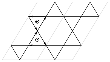
Figure 1: Bond directions for Dzyaloshinskii-Moriya interaction where the DM vector $\vec{D}$ (shown at the center of triangle) is staggered between up to down triangles.

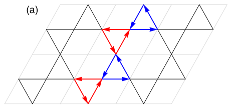
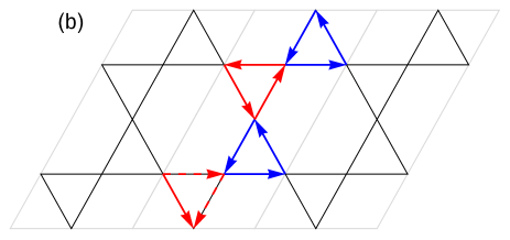
Figure 2: Grey lines mark the three-site unit cell for the $(0,0)$,$(\pi,0)$ Ansatz in the Fig. (a) and six-site unit cell for cuboc1 Ansatz in Fig. (b). The mean fields are defined as $\langle\mathcal{A}_{ij}\rangle=|\mathcal{A}|e^{i\phi_{\mathcal{A}}}$ and $\langle\mathcal{B}_{ij}\rangle=|\mathcal{B}|e^{i\phi_{\mathcal{B}}}$. In the Fig. (a), for $(0,0)$ Ansatz $\phi_{\mathcal{A}}=0$ for both the red (down) triangles and blue (up) triangles. For $(\pi,0)$ Ansatz $\phi_{\mathcal{A}}=0$ for red triangles and $\phi_{\mathcal{A}}=\pi$ for blue triangles. For both the Ansätze $\phi_{\mathcal{B}}=\pi$ for all bonds. In the Fig. (b), for $cuboc1$ Ansatz, $(\phi_{A},\phi_{B})=(\phi,\pi)$ for blue triangles where $\phi$ is arbitrary. For red triangles, for undashed lines $(\phi_{A},\phi_{B})=(0,\pi)$ and for dashed lines $(\phi_{A},\phi_{B})=(\pi,0)$ .

It is expected that the DM interaction will induce long range order and hence using SBMFT approach is appropriate since it elegantly treats both ordered and spin liquid phases. In Schwinger boson representation the spin operators are mapped to the bosonic operators as follows,

$$S^{\alpha}_{i} = \frac{1}{2}\begin{pmatrix}a_{i}^{\dagger}&b_{i}^{\dagger}\end{pmatrix}\sigma^{\alpha}\begin{pmatrix}a_{i}\\ b_{i}\end{pmatrix}$$ (2)

where $i$ is the site index and $\alpha={x,y,z}$. $\sigma^{\alpha}$ are the Pauli matrices. This mapping is faithful only when the number of bosons is equal to $2S$, that is, $(a_{i}^{\dagger}a_{i}+b_{i}^{\dagger}b_{i})=2S$. This constraint, in principle, must be satisfied at each site. However, it is interesting to study the properties of the bosonic system by implementing this constraint on average basis by treating $2S$ as a parameter. Let $\kappa=\braket{n_{i}}/2$ be the boson density per flavor. The spin wave function is then obtained by applying appropriate projection operator.

We define bond creation operators as $\hat{A}_{ij}^{\dagger}=\frac{1}{2}(e^{i\theta_{ij}}a_{i}^{\dagger}b_{j}^{\dagger}-e^{-i\theta_{ij}}b_{i}^{\dagger}a_{j}^{\dagger})$ and $\hat{B}^{\dagger}_{ij}=\frac{1}{2}(a_{i}a^{\dagger}_{j}+b_{i}b^{\dagger}_{j})$ with $\theta_{ij}=D_{ij}/J$. The operator $A^{\dagger}_{ij}$ creates a mixture of a singlet and a triplet on the bond, while $B^{\dagger}_{ij}$ is represents coherent hopping of the bosons between the sites. These definitions are slightly different from those used by Manuel et al Manuel et al. (1996). We can rewrite the Hamiltonian in terms of these bond operators with an approximation that $D/J$ is very small as,

$$H=\sum_{\langle ij\rangle}J\big{[}:\hat{B}_{ij}^{\dagger}\hat{B}_{ij}:-\hat{A}_{ij}^{\dagger}\hat{A}_{ij}\big{]}$$ (3)

where $::$ means normal order. We decouple the quartic term by introducing mean fields ${\cal{A}}_{ij}=\left\langle\hat{A}_{ij}\right\rangle$ and ${\cal{B}}_{ij}=\left\langle\hat{B}_{ij}\right\rangle$. Then the mean field hamiltonian is given by

$$H_{\text{MF}}=\sum_{\langle ij\rangle}J\big{[}\mathcal{B}_{ij}\hat{B}_{ij}^{\dagger}-\mathcal{A}_{ij}\hat{A}_{ij}^{\dagger}\big{]}+\text{H.C.}-\sum_{i}\lambda_{i}\hat{n}_{i}+\epsilon_{0}$$ (4)

where $\epsilon_{0}=\sum_{\langle ij\rangle}J(\mathcal{A}_{ij}|^{2}-|\mathcal{B}_{ij}|^{2})+2S\sum_{i}\lambda_{i}$. The Lagrange’s multiplier $\lambda_{i}$ has been added to constrain the mean boson number at each site.

The PSG analysis of $\mathbb{Z}_{2}$ spin liquids on kagome lattice was carried out by Wang and Vishwanath and they have shown that there are only four symmetric Ansätze possible Wang and Vishwanath (2006). They have labeled these Ansätze as $(0,0),(\pi,0),(0,\pi)$ and $(\pi,\pi)$, based on the fluxes through the hexagon and the rhombus. These Ansätze respect time reversal symmetry and lead to planar long range order. However, Messio et al have shown that ground state of Heisenberg antiferromagnet on kagome lattice is possibly a chiral spin liquid which is termed as cuboc1 Messio et al. (2012). A systematic enumeration of weakly symmetric spin liquids shows that there are 20 families of spin liquid Ansätze on kagome lattice Messio et al. (2013). We restrict our choices to the four symmetric spin liquids since DM interaction prefers planar LRO and cuboc1 spin liquid since it energetically most favorable in absence of DM interaction. In all Ansätze, the magnitudes of $\mathcal{A}_{ij}$ and $\mathcal{B}_{ij}$ are same on all bonds, that is, $\left|\mathcal{A}_{ij}\right|=\mathcal{A}$ and $\left|\mathcal{B}_{ij}\right|=\mathcal{B}$. $\mathcal{A}$ and $\mathcal{B}$ are complex numbers and their phases are summarized in the caption of the Fig. 2 below. It is also assumed that the Lagrange’s multiplier is independent of sites and is equal to $\lambda$. Using Fourier transformation, the Hamiltonian can be written as

$$H_{\text{MF}}=\sum_{q}\phi_{q}^{\dagger}N_{q}\phi_{q}+N\big{[}\lambda(2S+1)+2(\mathcal{A}^{2}-\mathcal{B}^{2})\big{]}$$ (5)

where $N$ is the number of sites and $\phi^{\dagger}_{q}=\big{[}a_{1q}^{\dagger},......a_{mq}^{\dagger},b_{1,-q},......b_{m,-q}\big{]}$. The first index $\mu$ in $a_{\mu q}$ and $b_{\mu q}$ is the sublattice index. $\mu$ can have values 1 to $m$ where $m$ is the number of sites per unit cell ($m=3$ for the $(0,0),(\pi,0)$ Ansätze and $m=6$ for cuboc1 Ansatz) and $N_{q}$ is a $2m\times 2m$ matrix.

This $N_{q}$ matrix can be diagonalised by Bogoliubov transformation $\phi_{q}=M_{q}\xi_{q}$, where $\xi^{\dagger}_{q}=\big{[}\alpha_{1q}^{\dagger},......\alpha_{mq}^{\dagger},\beta_{1,-q},......\beta_{m,-q}\big{]}$. The transformation matrix must satisfy $M_{q}\tau M_{q}^{\dagger}=\tau$ where $\tau=\sigma_{3}\otimes I_{m}$. We must find $M_{q}$ such that $M_{q}^{\dagger}N_{q}M_{q}=\Omega_{q}$ where $\Omega_{q}=\text{diag}(\omega^{\alpha}_{\mu q}..........,\omega^{\beta}_{\mu,-q})$. The form of the $M_{q}$-matrix is given by $M_{q}=\begin{bmatrix}U_{q}&X_{q}\\ V_{q}&Y_{q}\end{bmatrix}$ where $U_{q},V_{q},X_{q}$ and $Y_{q}$ are the $m\times m$ matrix.

The diagonalised hamiltonian is given by

$$H_{\text{MF}} = \sum_{q}\sum_{\mu}\big{(}\omega_{\mu q}^{\alpha}\alpha_{\mu q}^{\dagger}\alpha_{\mu q}+\omega_{\mu q}^{\beta}\beta_{\mu q}\beta_{\mu q}^{\dagger}\big{)}$$ (6)

$$+ N\big{[}\lambda(2S+1)+2(\mathcal{A}^{2}-\mathcal{B}^{2})\big{]}$$

where $\omega^{\alpha}_{\mu q}$ and $\omega^{\beta}_{\mu q}$ are the excitation energies of $2m$ spinon modes. Note that for chiral Ansatz $\omega_{\mu q}^{\alpha}\neq\omega_{\mu q}^{\beta}$. The ground state energy is given by

$$E=\sum_{q,\mu}\omega_{\mu q}^{\beta}+N\big{[}\lambda(2S+1)+2(\mathcal{A}^{2}-\mathcal{B}^{2})\big{]}$$ (7)

Bogolioubov matrix is computed using the procedure outlined in ref Colpa (1978). The mean field parameters $\mathcal{A},\mathcal{B},\lambda$, and $\phi$ are found by extremizing the ground state energy $E$. The positive definiteness of the Hamiltonian puts several conditions on the domain of these parameters. The method used for searching the saddle points is outlined in the next section. The complex link variables $\mathcal{A}_{ij}$ and $\mathcal{B}_{ij}$ satisfies the self consistency equations

$$\mathcal{A}_{ij}=\braket{\hat{\mathcal{A}}_{ij}}\hskip 14.22636pt\text{\&}\hskip 14.22636pt\mathcal{B}_{ij}=\langle\hat{\mathcal{B}}_{ij}\rangle$$ (8)

which are equivalent to extremization of free energy as

$$\frac{\partial E}{\partial\mathcal{A}}=\frac{\partial E}{\partial\mathcal{B}}=\frac{\partial E}{\partial\mathcal{\phi}}=\frac{\partial E}{\partial\lambda}=0$$ (9)

III Numerical search for saddle points

The bosonic mean field Hamiltonian is diagonalizable if $N_{q}$ is positive definite for all $q$. We begin the search by finding the valid domain in parameter space $\{\mathcal{A},\mathcal{B},\lambda\}$ where this conditions is true. The gapless LRO phases emerge as the corresponding saddle point approaches the boundaries, thus closing the gap in the spinon spectrum. These points are difficult to find since the eigenvalues of the Hessian has drastic varying magnitudes at the saddle point. As an example we have given the Hessian matrix of Ansatz $(\pi,0)$ at $S=0.366,\theta=0.21$ and $N=20$

$$h=\left(\begin{array}[]{ccc}0.9230&-0.5794&-1.0186\\ -0.5794&-3.6344&-0.3558\\ -1.0186&-0.3558&-9.9997\times 10^{11}\\ \end{array}\right)$$

The eigenvalues of $h$ are given by $\{-9.9997\times 10^{11},-3.7069,0.9955\}$. Thus in LRO phases, we rotate co-ordinate axes which are nearly parallel to the eigenvectors of the Hessian, two of which are parallel to the boundary surface. The main hurdle in this procedure is to finding boundary surfaces. However these can be guessed by examining the classical orders. Thus analyzing eigenvalues of $N_{q}$ at few high symmetry points in reciprocal lattice is enough. For $\sqrt{3}\times\sqrt{3}$ phase, the boundary plane is given by

$$\sqrt{3}|\cos\theta|\mathcal{A}+\mathcal{B}+\lambda=0$$ (10)

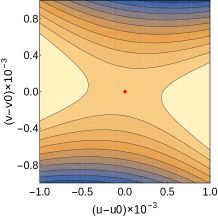
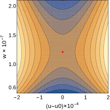
Figure 3: Optimum points $(u0,v0,w0)$ in the rotated frame $(u,v,w)$ for Ansatz $(\pi,0)$ at $S=0.366$ and $\theta=0.21$

The boundary surfaces in cuboc1 state are not planner but then it is still possible to search for saddle point along the surfaces and then perpendicular direction. This way we have been able to achieve much better accuracy where the sum of squares of gradients is of the order of $10^{-14}$

IV PROPERTIES AND THE PHASE DIAGRAM

We have computed energies for various values of $\kappa\,(0\text{ to }0.5)$ and $\theta\,(0\text{ to }\pi/6)$ for all Ansätze. Based on the energy and the gap in the spinon spectrum, our proposed ground state phase diagram is shown in the Fig. 4. As expected, for low values of $\kappa$ and also small strengths of DM interaction, the phases are gapped spin liquids. For $\theta\lesssim 0.5$, the gap in the spinon spectrum closes at about $\kappa=0.39$ indicating a second ordered transition from gapped liquid phase to gap-less cuboctahedral LRO. For large strength of DM interaction, that is for $\theta>0.2$, the system enters $\mathbf{Q}=0$ LRO phase at $\theta\gtrsim 0.2$. Fig. 5 shows that the gap closes at $\kappa=0.18$ for $\theta=0.3$.

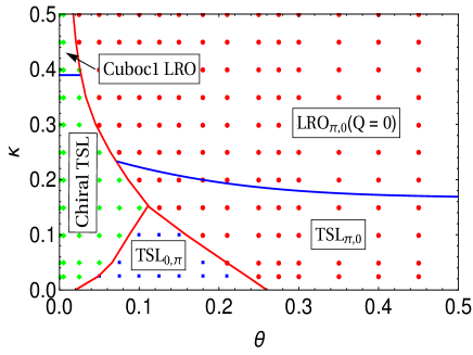
Figure 4: Ground State phase diagram at $T=0$. In the phase diagram indicate second ordered phase transitions are shown in blue and the first ordered transitions by red lines.

To illustrate the nature of various phases we also have calculated static spin structure factor

$$S^{\alpha\alpha}(\textbf{Q})=\frac{3}{4N}\sum_{i,j}q^{i\textbf{Q}\cdot(\textbf{R}_{i}-\textbf{R}_{j})}\langle 0|S_{i}^{\alpha}S_{j}^{\alpha}|0\rangle$$

where $\alpha={x,y,z}$, $\textbf{R}_{i}$ and $\textbf{R}_{j}$ are the positions of the site $i$ and $j$. Due to DM interaction, the global spin rotation symmetry is reduced to $U(1)$, and hence one must calculate both $S^{xx}$ and $S^{zz}$. The expressions for the structure factor in terms of Bogoliubov matrices is given in appendix.

IV.1 Spin Liquid Phases

The phases of the isotropic Heisenberg model ($\theta=0$) have been studied by Messio and our results are matching with them. For $\kappa>0.39$, the spinon spectrum is gap-less at $\mathbf{Q}=\frac{3}{2}\mathbf{K}$. At $\kappa\leq 0.39$, the gap opens up and the system enters chiral spin liquid phase and remains in this phase down to $\kappa=0$. Fig. 5 shows the variation of energy gap as a function of $\kappa$. However it is interesting to note that the short range correlations are cuboctahedral near the phase transition but as $\kappa$ is decreased the peak in static structure factor becomes broad but also shift towards $\mathbf{K}$ point (Fig. 6(a)) before flattening out at $\kappa=0.1$. Thus the short range correlations become more like $\sqrt{3}\times\sqrt{3}$ type as $\kappa$ is decreased which is consistent with $q_{1}=-q_{2}$ spin liquid state obtained by Sachdev Huh et al. (2010).

Figure 5: Variation of energy gap with $\kappa$ for cuboc1 Ansatz at $\theta=0$ and $(0,\pi)$ Ansatz at $\theta=0.30$

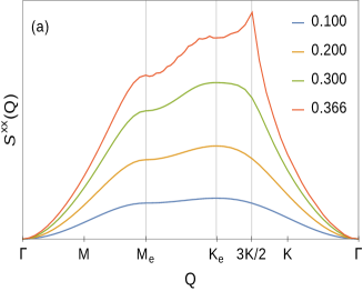
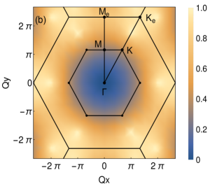
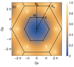
Figure 6: (a) XX-component of static structure factor along the high symmetry line $\bf{\Gamma}-M_{e}-K_{e}-\Gamma$ for cuboc1 Ansatz for different values of $\kappa$ at $\theta=0$. XX-component of static structure factor for cuboc1 Ansatz at (b) $S=0.366$ and $\theta=0$ (c) $S=0.5$ and $\theta=0$

For small values of boson density, $\kappa(<0.15)$, the quantum fluctuations prevent any sort of long range order in the system even in presence of strong DM interaction. For very small values of $\theta$, the system persists in cuboc1 spin liquid phase before making a first order transition to $(0,\pi)$ spin liquid phase. In this phase, the static structure factor again shows a very broad peak at $\mathbf{K}$ point. As the strength of the DM interaction is further increased the system enters $(\pi,0)$ spin liquid phase with the short range correlations of type $\boldsymbol{Q}=0$ showing a broad peak in spin structure factor at $\mathbf{M}_{e}$ point. Comparison with the phase diagram obtained by Messio, this transition occurs at much smaller values of DM interaction. This indicates the inclusion of $\mathcal{B}$ fields helps stabilizing $(\pi,0)$ spin liquid against $(0,\pi)$ phase.

IV.2 Neel Ordered Phases

For very small values of DM interaction and $\kappa>0.39$, all three Ansätze $\left(0,0\right)$, $\left(0,\pi\right)$ and cuboc1 are all in gapless phases corresponding to classical orders $\sqrt{3}\times\sqrt{3}$ , $\boldsymbol{Q}=0$ and cuboctahedral respectively Messio et al. (2011). However the lowest energy in cuboc1 Ansatz. In this phase, the soft modes in spinon spectrum are at $\frac{3}{4}\mathbf{K}$ points in extended Brillouin zone. Even though the Ansatz is still symmetric, the mechanism of symmetry breaking leading to emergence long range order through bose condensation is well understood and is described in Sachdev Sachdev (1992) and Messio Messio et al. (2013). The spin structure factor in this phase shows strong peaks at $\frac{3}{2}\mathbf{K}$ point which confirms the cuboc1 LRO phase (Fig. 6(c)). At $\kappa=\frac{1}{2}$, the system is in cuboc1 LRO phase for $\theta<0.0173$ and then enters $\boldsymbol{Q}=0$ phase with a first order phase transition. This width of cuboc1 LRO decreases as $\kappa\to\infty$ where even infinitesimal DM interaction immediately orders the system in planar configuration.

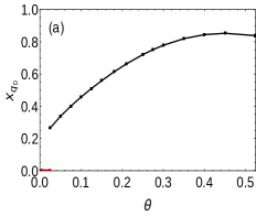
Figure 7: Condensate fraction $x_{q_{0}}$ as a function of $\theta$ (a) in the ground state at $\kappa=0.366$ where the red points shows cuboc1 Ansatz and black points shows $(\pi,0)$ Ansatz (b) for $\left(\pi,0\right)$ Ansatz at $S=0.2$

For $\theta>0.1$, the $\left(\pi,0\right)$ spin liquid shares a phase boundary with the $\mathbf{Q}=0$ phase, which is favored by DM interaction. Across this boundary, the gap closes at $Q=0$. The signature sharp peaks in static structure factor at $\mathbf{M}_{e}$ point. The condensate fraction $x_{0}$ in soft mode at $q_{0}$ can be computed using

$$\frac{1}{2S}\sum_{i}\langle n_{i}\rangle=x_{q_{0}}N+\sum_{\begin{subarray}{c}j,i\neq i_{0}{}\\ q\neq q_{0}\end{subarray}}\frac{|V_{ij}(q)|^{2}}{S}.$$

Fig. 7(a) shows the emergence of the condensate fraction as a function of $\theta$ along the $\kappa=0.366$ horizontal line in the phase diagram. condensate fraction is zero in the cuboc1 Ansatz and becomes nonzero for the $(\pi,0)$ Ansatz via first order phase transition at $\theta\approx 0.03$. In the Fig. 7(b), for $S=0.2$ the second order phase transition occurs near $\theta=0.15$ for $(\pi,0)$ Ansatz.

IV.3 Discussion

The ground state phase diagram obtained here is qualitatively similar to that of Messio Messio et al. (2010) except that the cuboc1 Ansatz replaces the $\left(0,0\right)$ Ansatz in the phase diagram. The results obtained at $\kappa=1/2$ however are not in agreement with earlier studies for spin 1/2 system Cépas et al. (2008); Laeuchli and Lhuillier (2009); Huh et al. (2010) which predict a moment-free phase for small values of $\theta$ and a second ordered phase transition to $\mathbf{Q}=0$ phase. However the nature of the short range correlations in liquid phase is unclear. Cepas et al argue that short range corrleations of type $\mathbf{Q}=0$, whereas Huh et al showed it to be of $\sqrt{3}\times\sqrt{3}$ type. However, Messio Messio et al. (2012) have argued that, in SBMFT, since $n_{i}=2S$ constraint is implemented only in an average sense, spin $1/2$ system may not be correctly represented by $\kappa=1/2$. Due to the fluctuations in $n_{i}$, the $\left\langle\boldsymbol{S}_{i}^{2}\right\rangle$ is overestimated to be $\frac{3}{2}S(S+1)$ at $\theta=0$. If we treat $\left\langle\boldsymbol{S}_{i}^{2}\right\rangle$ to be a good quantum number, then the spin $1/2$ system is approximated by the bosonic system at $\kappa=0.366$. At this value of $\kappa$, our proposal shows that the system is $\mathbb{Z}_{2}$ chiral spin liquid till $\theta<0.03$ with short range correlations of cuboctahedral kind. For $\theta>0.03$, the DM interaction forces the spins to be in planar arrangement with $\boldsymbol{Q}=0$ long range order.

It is also possible that the best representation may be at smaller values of $\kappa$, where we have noted that the short range correlations tend to be more like $\sqrt{3}\times\sqrt{3}$ type as argued by Messio et al. Even though at $\kappa=0.366$ shows a first order transition from spin liquid to $\mathbf{Q}=0$ LRO, it may not be adequate in reconciling with the experimental results. The strength of the DM interaction is estimated to be $0.08J$ in $\mathrm{ZnCu}_{3}(\mathrm{OH})_{6}\mathrm{Cl}_{3}$. This compound does not exhibit freezing of magnetic moments to very low temperatures Helton et al. (2007). In the present mean field theory, at $\kappa=0.366$, the critical $D_{c}=0.03J$. The optimized value of mean field parameters and energy for $S=0.366$ is as given in the table below.

Ansatz	$\theta$	$\mathcal{A}$	$\mathcal{B}$	$\lambda$	$\phi$	energy
cuboc1	0	0.4036	0.1185	-0.5803	1.9847	-0.2976
$(\pi,0)$	0.21	0.4226	0.1340	-0.6700	-	-0.3213

Table 1: Optimized values and energies for different Ansätze

V Dynamical spin structure factor

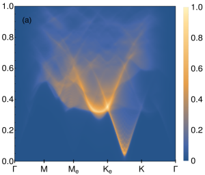
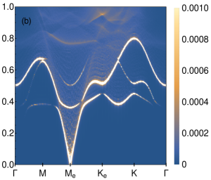
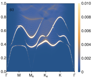
Figure 8: XX-component of dynamical structure factor for (a) $cuboc1$ Ansatz at $S=0.366$ and $\theta=0$ (b) $(\pi,0)$ Ansatz at $S=0.366$ with $\theta=0.21$ (c) ZZ-component of dynamical structure factor for $(\pi,0)$ Ansatz at $S=0.366$ and $\theta=0.21$. In LRO phase we choose scale to be very small such that the spinon continuum is visible.

Since in neutron scattering experiment the inelastic neutron scattering cross section is proportional to the dynamical spin structure factor, we have calculated the dynamical spin structure factor defined by

$$S^{\alpha\alpha}(\textbf{Q},\omega)=\int_{-\infty}^{\infty}\langle 0|S_{-\textbf{Q}}^{\alpha}(t)S_{\textbf{Q}}^{\alpha}(0)|0\rangle e^{i\omega t}dt$$ (11)

where $\alpha={x,y,z}$ and $|0\rangle$ is the ground state of the system . The expressions for ZZ and XX component of dynamical structure factor in terms of Bogoliubov matrices are given in the appendix. For numerical purpose, the delta function is approximated by Lorentzian function. The results are qualitatively similar to the results obtained by Messio.

In the figure, we illustrate the evolution of the dynamical structure factor across the phase transition from spin liquid to LRO phase for $\kappa=0.366$. The dynamical structure factor is shown along the high symmetry line $\mathbf{\Gamma}-\mathbf{M}_{e}-\mathbf{K}_{e}-\mathbf{\Gamma}$. The dynamical structure factor of cuboc1 Ansatz at $\theta=0$ in Fig. 8(a) shows sharp onset of spinon continum at $\frac{3}{2}\mathbf{K}$ with very small gap. This is due to the proximity of critical point at $\kappa=0.39$ beyond which there is cuboc1 long range order.

Since the DM interaction reduces the global spin rotation symmetry from $SU(2)$ to $U(1)$, there is notable difference between XX and ZZ component of dynamical structure factor. In Fig. 8(b) and Fig. 8(c), we show the dynamical structure factor of Ansatz $(0,\pi)$ at $\theta=0.21$ which is $\mathbf{Q}=0$ LRO phase.

In the XX-component of dynamical structure factor, the magnon branches are quite strong and in the the density plot, it is visible as three lines of bright dots corresponding to three magnon branches. These magnon branches are obtained by considering the pair of spinons, one in the soft modes and other one from the excited state. The elastic peak (along $\omega=0$ line) appears with largest intensity at $\mathbf{M}_{e}$ point which is the $\mathbf{\Gamma}$ point of the next wigner- seitz cell.

In the ZZ-component of dynamical structure factor the magnon branches are of very low intensity and suppressed, as the spins are forced to lie in the XY plane due to the DM interaction.

VI Conclusion

We have computed the ground state phase diagram of Heisenberg Kagome antiferromagnet with DM interaction using SBMFT approach. We have included the time reversal symmetry breaking chiral Ansatz proposed by Messio Messio et al. (2012)and also considered hopping mean field $\mathcal{B}$. For large $S$, even with small DM interaction, the spins are forced to in plane and in $\mathbf{Q}=0$ long range order. For small $S$, the quantum fluctuations induce series of spin liquid phases with increasing DM interaction. In this region, the inclusion of the hopping field seems to stabilize $(\pi,0)$ spin liquid phase over $(0,\pi)$ spin liquid.

Since the constraint of boson density is implemented strictly, $\braket{\mathbf{S}_{i}^{2}}=\frac{1}{2}$ at $\kappa=0.366$ due to the fluctuations in boson density. We find that, at $\kappa=0.366$, the model shows a first ordered phase transition from chiral cuboc1 spin liquid to $\mathbf{Q}=0$ Neel phase at $D=0.03J$. Even though, this result is qualitatively in agreement with other studies, it is not adequate in explaining the moment free phase of Herbertsmithite Helton et al. (2007) since the estimated DM strength is $0.08J$. Probably, one may need to consider even smaller values of $\kappa$ to obtain better numerical agreement with other studies and experiment. We, have also calculated static and dynamical structure factor at the representative $\kappa=0.366$ point.

VII APPENDIX

VII.1 Static spin structure factor

The expression for XX-component of static spin structure factor is given by

$$S^{xx}(\mathbf{Q}) = \frac{3}{16N}\sum_{q,\mu\nu}\Big{[}[X_{\mathbf{Q}+q}^{*}Y_{\mathbf{Q}+q}^{T}]_{\mu\nu}[Y_{-q}^{*}X_{-q}^{T}]_{\mu\nu}$$ (12)

$$+ [X_{\mathbf{Q}+q}^{*}X_{\mathbf{Q}+q}^{T}]_{\mu\nu}[Y_{-q}^{*}Y_{-q}^{T}]_{\mu\nu}$$

$$+ [V_{q}U_{q}^{\dagger}]_{\mu\nu}[U_{-\mathbf{Q}-q}V_{-\mathbf{Q}-q}^{\dagger}]_{\mu\nu}$$

$$+ [V_{-\mathbf{Q}-q}V_{-\mathbf{Q}-q}^{\dagger}]_{\mu\nu}[U_{q}U_{q}^{\dagger}]_{\mu\nu}\Big{]}$$

The ZZ- component of structure factor has the form

$$S^{zz}(\textbf{Q}) = \frac{3}{16N}\sum_{q,\mu,\nu}\Big{[}[X_{{\textbf{Q}}+q}^{*}X_{{\textbf{Q}}+q}^{T}]_{\mu\nu}[U_{q}U_{q}^{\dagger}]_{\mu\nu}\Big{]}$$ (13)

$$+ [V_{-{\textbf{Q}}-q}V_{-{\textbf{Q}}-q}^{\dagger}]_{\mu\nu}[X_{-q}^{*}X_{-q}^{T}]_{\mu\nu}$$

$$- [X_{{\textbf{Q}}+q}^{*}Y_{{\textbf{Q}}+q}^{T}]_{\mu\nu}[U_{q}V_{q}^{\dagger}]_{\mu\nu}$$

$$- [V_{-{\textbf{Q}}-q}U_{-{\textbf{Q}}-q}^{\dagger}]_{\mu\nu}[Y_{-q}^{*}X_{-q}^{T}]_{\mu\nu}$$

VII.2 Dynamical spin structure factor

The expression for XX-component of dynamical spin structure factor is given by

$$S^{xx}(\textbf{Q},\omega) = 2\pi\sum_{q}\sum_{\mu\nu}\Big{[}|[U_{q}^{\dagger}V_{-q-{\textbf{Q}}}^{*}]_{\mu\nu}+[U_{-q-{\textbf{Q}}}^{\dagger}V^{*}_{q}]_{\nu\mu}|^{2}$$ (14)

$$+ |[Y_{-q}^{T}X_{q+{\textbf{Q}}}]_{\mu\nu}+[Y_{{\textbf{Q}}+q}^{T}X_{-q}]_{\nu\mu}|^{2}\Big{]}$$

$$\times \delta(\omega-\omega_{p})$$

where $\mu,\nu$ are the sublattice index. The expression for ZZ-component of dynamical spin structure factor reduces to

$$S^{zz}(\textbf{Q},\omega) = 2\pi\sum_{q}\sum_{\mu\nu}|\big{[}U_{q}^{\dagger}X_{{\textbf{Q}}+q}\big{]}_{\mu\nu}-\big{[}V_{q}^{\dagger}Y_{{\textbf{Q}}+q}\big{]}_{\mu\nu}|^{2}$$ (15)

$$\times \delta(\omega-\omega_{p})$$

where $\omega_{p}=\omega_{q}+\omega_{-{\textbf{Q}}-q}$. At ${\textbf{Q}}=0$ the $zz$-component will straight way will give zero because it is just the dot product of the two columns of the M matrix(para orthogonalization), consistent with the figure.

References

- Anderson (1973) P. Anderson, Materials Research Bulletin 8, 153 (1973).
- Lhuillier and Misguich (2011) C. Lhuillier and G. Misguich, in Introduction to Frustrated Magnetism (Springer, 2011) pp. 23–41.
- Mila (2000) F. Mila, European Journal of Physics 21, 499 (2000).
- Balents (2010) L. Balents, Nature 464, 199 (2010).
- Savary and Balents (2016) L. Savary and L. Balents, Reports on Progress in Physics 80, 016502 (2016).
- Leung and Elser (1993) P. W. Leung and V. Elser, Phys. Rev. B 47, 5459 (1993).
- Yan et al. (2011) S. Yan, D. A. Huse, and S. R. White, Science 332, 1173 (2011).
- Jiang et al. (2008) H. C. Jiang, Z. Y. Weng, and D. N. Sheng, Phys. Rev. Lett. 101, 117203 (2008).
- Ran et al. (2007) Y. Ran, M. Hermele, P. A. Lee, and X.-G. Wen, Phys. Rev. Lett. 98, 117205 (2007).
- Dzyaloshinskii (1957) I. Dzyaloshinskii, Sov. Phys. JETP 5 (1957).
- Moriya (1960) T. Moriya, Physical Review 120, 91 (1960).
- Helton et al. (2007) J. Helton, K. Matan, M. Shores, E. Nytko, B. Bartlett, Y. Yoshida, Y. Takano, A. Suslov, Y. Qiu, J.-H. Chung, et al., Phys. Rev. Lett. 98, 107204 (2007).
- Lee (2008) P. A. Lee, Science 321, 1306 (2008).
- Levi (2007) B. G. Levi, Physics today 60, 16 (2007).
- Zorko et al. (2008) A. Zorko, S. Nellutla, J. Van Tol, L. Brunel, F. Bert, F. Duc, J.-C. Trombe, M. De Vries, A. Harrison, and P. Mendels, Phys. Rev. Lett. 101, 026405 (2008).
- Rigol and Singh (2007) M. Rigol and R. R. Singh, Phys. Rev. Lett. 98, 207204 (2007).
- Rousochatzakis et al. (2009) I. Rousochatzakis, S. R. Manmana, A. M. Läuchli, B. Normand, and F. Mila, Physical Review B 79, 214415 (2009).
- Cépas et al. (2008) O. Cépas, C. Fong, P. W. Leung, and C. Lhuillier, Phys. Rev. B 78, 140405 (2008).
- Tovar et al. (2009) M. Tovar, K. S. Raman, and K. Shtengel, Physical Review B 79, 024405 (2009).
- Hermele et al. (2008) M. Hermele, Y. Ran, P. A. Lee, and X.-G. Wen, Physical Review B 77, 224413 (2008).
- Messio et al. (2010) L. Messio, O. Cépas, and C. Lhuillier, Phys. Rev. B 81, 064428 (2010).
- Huh et al. (2010) Y. Huh, L. Fritz, and S. Sachdev, Phys. Rev. B 81, 144432 (2010).
- Messio et al. (2012) L. Messio, B. Bernu, and C. Lhuillier, Phys. Rev. Lett. 108, 207204 (2012).
- Mezio et al. (2011) A. Mezio, C. Sposetti, L. Manuel, and A. Trumper, Europhys. Lett.) 94, 47001 (2011).
- Flint and Coleman (2009) R. Flint and P. Coleman, Physical Review B 79, 014424 (2009).
- Manuel et al. (1996) L. Manuel, C. Gazza, A. Trumper, and H. Ceccatto, Phys. Rev. B 54, 12946 (1996).
- Wang and Vishwanath (2006) F. Wang and A. Vishwanath, Phys. Rev. B 74, 174423 (2006).
- Messio et al. (2013) L. Messio, C. Lhuillier, and G. Misguich, Phys. Rev. B 87, 125127 (2013).
- Colpa (1978) J. Colpa, Physica A: Statistical Mechanics and its Applications 93, 327 (1978).
- Messio et al. (2011) L. Messio, C. Lhuillier, and G. Misguich, Phys. Rev. B 83, 184401 (2011).
- Sachdev (1992) S. Sachdev, Phys. Rev. B 45, 12377 (1992).
- Laeuchli and Lhuillier (2009) A. Laeuchli and C. Lhuillier, (2009), 0901.1065 .