Clues to the origin and properties of magnetic white dwarfs

Abstract

A significant fraction of white dwarfs possess a magnetic field with strengths ranging from a few kG up to about 1000 MG. However, the incidence of magnetism varies when the white dwarf population is broken down into different spectral types providing clues on the formation of magnetic fields in white dwarfs. Several scenarios for the origin of magnetic fields have been proposed from a fossil field origin to dynamo generation at various stages of evolution. Offset dipoles are often assumed sufficient to model the field structure, however time-resolved spectropolarimetric observations have revealed more complex structures such as magnetic spots or multipoles. Surface mapping of these field structures combined with measured rotation rates help distinguish scenarios involving single star evolution from other scenarios involving binary interactions. I describe key observational properties of magnetic white dwarfs such as age, mass, and field strength, and confront proposed formation scenarios with these properties.

1 Introduction

Following the discovery of a magnetic field in 78 Virginis ([Babcock (1947), Babcock 1947]), [Blackett (1947), Blackett (1947)] contemplated the presence of stronger magnetic fields in white dwarfs assuming magnetic flux conservation throughout evolution. The strong circular polarization spectrum of the first known magnetic white dwarf, Grw+70^∘ 8247 ([kem1970, Kemp et al. 1970]), implied a longitudinal field measurement of $\approx 10^{7}$ G, which was nearly a thousand times the field strength observed in Ap stars at the time. Following the original discovery, many more magnetic white dwarfs were found with strong magnetic fields ($B\gtrsim 10^{7}$ G) including G195-19 as the prototype for the cool, continuum-like, helium-rich magnetic white dwarfs (DCP, [Angel & Landstreet (1971), Angel & Landstreet 1971]) and G99-37 as the prototype for carbon-enriched magnetic white dwarfs (DQP but originally classified as DGp, [Greenstein (1969), Greenstein 1969], [Landstreet & Angel (1971), Landstreet & Angel 1971]). Early observations already demonstrated that magnetic fields are present across all spectral types. Although a search for lower strength magnetic fields ($\lesssim 5$ MG) carried out by [Angel, Borra & Landstreet (1981), Angel, Borra & Landstreet (1981)] proved negative, the number of white dwarfs with magnetic fields greater than 1 MG steadily grew by 1995 to 40 objects (see [Schmidt & Smith (1995), Schmidt & Smith 1995]). Spectropolarimetric measurements proved capable of reaching below 1 MG field strength with the discovery of two low-field white dwarfs (0.1 MG) in a large survey of 170 objects ([Schmidt & Smith (1994), Schmidt & Smith (1995), Schmidt & Smith 1994,1995]). With even larger surveys, such as the Sloan Digital Sky Survey (SDSS) and with larger telescopes and more sensitive instruments, the number of magnetic white dwarfs has grown to over 600 (see, e.g., [Ferrario, de Martino & Gänsicke (2015), Ferrario, de Martino & Gänsicke 2015]) but still including only 18 objects with fields below 1 MG ([Kawka & Vennes (2012), Kawka & Vennes 2012], [Landstreet, et al. (2017), Landstreet, et al. 2017]).

This paper aims to summarise our current understanding of the magnetic white dwarf population and the methods used to detect and determine magnetic fields in white dwarfs (Section 2). The properties of the magnetic white dwarf population are presented in Section 3 and the various models for the origin of magnetic fields in white dwarfs are presented in Section 4. Finally, Section 5 exposes current challenges in modelling magnetic atmospheres in particular the effect of magnetic fields on convective motion and the atmospheric structure.

2 Measuring magnetic field strengths

There are two complementary ways to detect and measure magnetic fields. The most straight forward follows the detection of Zeeman splitted lines. Depending on the atomic structure and magnetic field strength, the Zeeman effect can be calculated using distinct methods. Fig. 1 shows examples of the different classes of magnetic white dwarfs. The magnetic DC white dwarfs, which have featureless spectra, are not included in the plot. The magnetic DQ shown is WD 2154-512 which exhibits CH molecular bands in its spectrum (shown in the left panel of Fig. 1 and centred at 4330 Å) and which were used in measuring its magnetic field strength from spectropolarimetry ([Berdyugina, Berdyugin & Piirola (2007), Berdyugina et al. 2007]). The figure also shows the different regimes of the Zeeman effect on various elements.

Figure 1: Example spectra showing the different spectral classes for which magnetism has been detected. The left panel shows the optical spectra. The left panel highlights a particular feature that is representative of the spectral type which is centred on the given wavelength. The absorption line at 5120 Å, marked with a star, in SDSSJ1018$+$0111 is an example of a stationary feature. In this case it is a Zeeman component of H$\beta$.

The normal Zeeman effect occurs when a spectral line of an atom with zero spin ($S=0$) splits into three components when immersed in a magnetic field. In this case, we can calculate the magnetic field strength using:

$$\Delta\lambda=\frac{eB\lambda^{2}}{4\pi m_{e}c^{2}}\approx 4.67\times 10^{-7}\lambda^{2}B$$ (1)

where $\lambda$ is the wavelength in Å, $B$ is the magnetic field in MG, $e$ is the electron charge (e.s.u.), $m_{e}$ is the electron rest mass, and $c$ is the speed of light.

The anomalous Zeeman effect depends on the electron spin and occurs in atoms with non-zero spin. The splitting in this regime can be complex and is observed at lower field strength where the spin and orbital angular momenta remain coupled. In general, the energy level of an electron can be described by three quantum numbers, $J$ which is the total angular momentum, $L$ which is the orbital angular momentum, and $S$ which is the spin orbital momentum. When an atom is placed in a magnetic field its levels split into $2J+1$ components. These are defined by the magnetic quantum number $m=-J,-J+1,...,J-1,J$ and the Zeeman shifted lines can be calculated using:

$$\Delta\lambda=\frac{eB\lambda^{2}}{4\pi m_{e}c^{2}}(g_{l}m_{l}-g_{u}m_{u})\approx 4.67\times 10^{-7}\lambda^{2}B(g_{l}m_{l}-g_{u}m_{u})$$ (2)

where $m_{u}$ and $m_{l}$ are the magnetic quantum numbers of the upper and lower levels, respectively. The permitted transitions are defined by $\Delta m=0,\pm 1$. Here, $\Delta m=0$ defines the $\pi$ components and $\Delta m=\pm 1$ the $\sigma$ components. The Landé factors for the upper and lower levels are $g_{u}$ and $g_{l}$, respectively and they can be calculated assuming LS coupling:

$$g=1+\frac{J(J+1)-L(L-1)+S(S+1)}{2J(J+1)},$$ (3)

The LS coupling is generally valid for lighter atoms such as sodium, magnesium, aluminium and calcium. For heavier atoms like iron LS coupling is no longer valid and other coupling needs to be applied. The Vienna Atomic Line Database provides atomic data including Landé factors for light and heavy elements.

The Paschen-Back effect occurs when the $m_{l}$ degeneracy is removed. In this regime the spin and orbital angular momenta decouple and the anomalous Zeeman effect reverts to the normal or linear Zeeman effect and Eqn. 1 can be used. The linear Zeeman splitting of hydrogen atoms falls into this regime.

As the magnetic field strength increases, the quadratic effect begins to take over. In this regime, the $l$ degeneracy is also removed and shifts in the $\pi$ components and asymmetry in the line profiles are observed. Increasing the field strength will cause even more complex Zeeman patterns and for more detail on these higher field regimes see [Ferrario, Wickramasinghe & Kawka (2019), Ferrario et al. (2019)]. [Landi Degl’Innocenti & Landolfi (2004), Landi Degl’Innocenti & Landolfi (2004)] present conveniently written Zeeman splitting formulae for the low field regime and quadratic effect. For further reading consult [Herzberg (1945), Herzberg (1945)]. Table 1 lists references to available calculations of line shifts and transition probabilities for hydrogen and helium at stronger magnetic fields, as well as some heavier elements such as sodium, calcium and carbon. For helium, the calculations of [Becken & Schmelcher (2001), Becken & Schmelcher (2001)] and [Al-Hujaj & Schmelcher (2003), Al-Hujaj & Schmelcher (2003)] supersede the calculations of [Kemic (1974), Kemic (1974)] and allowed the measurement of magnetic field strengths of strongly magnetic DB white dwarfs ([Jordan, et al. (1998), Wickramasinghe, et al. (2002), Jordan et al. 1998, Wickramasinghe et al. 2002]). Measuring magnetic field strengths at high fields ($\gtrsim 100$ MG) can be difficult due to the complexity of the Zeeman pattern. Also, the magnetic field on a white dwarf surface is not uniform and can vary significantly, up to a factor of two even if a simple dipole is assumed. This can smear out most of the absorption features, however some line components become stationary where the wavelength goes through a minimum or maximum as a function of the field strength. These stationary components can be observed in spectra even when the field varies considerably (see Fig 1).

Table 1: Calculations of Zeeman splitted lines.

Element	$B$ Range (G)	Spectral range	Reference
Hydrogen	$0-5\times 10^{12}$	Lyman, Balmer, Paschen, Brackett	[Schimeczek & Wunner (2014), Schimeczek & Wunner (2014)]
Helium	$0-2.35\times 10^{11}$	HeI	[Becken & Schmelcher (2001), Becken & Schmelcher (2001)]
Helium	$2.35\times 10^{11}-2.35\times 10^{13}$	HeI	[Al-Hujaj & Schmelcher (2003), Al-Hujaj & Schmelcher (2003)]
Sodium	$0-4.7\times 10^{7}$	$n=3-7$	[González-Férez & Schmelcher (2003), González-Férez & Schmelcher (2003)]
Calcium	$10^{6}-10^{8}$	CaII H&K	[Kemic (1975), Kemic (1975)]

Spectropolarimetric measurements add additional geometric information following a magnetic field detection. To date, most spectropolarimetric observations have measured the circular polarization, the Stokes parameter $V$. The longitudinal field strength ($B_{l}$ in G) can be determined using:

$$v=\frac{V}{I}=\frac{dI}{d\lambda}\frac{4.67\times 10^{-13}\lambda^{2}B_{l}}{I}$$ (4)

This equation provides for a determination of the longitudinal field strength from the measured polarization $V$ and the intensity spectrum $I$ for stars where the Zeeman splitting is smaller than the width of the line profile. Several low field DA white dwarfs have been recently detected using this technique ([Kawka & Vennes (2012), Landstreet & Bagnulo (2019), Landstreet & Bagnulo (2019), e.g., Kawka & Vennes 2012, Landstreet & Bagnulo 2019]). Fig. 2 shows the H$\beta$ line profile of the weakly magnetic NLTT 2219 as well as the circular polarization spectrum showing the polarized $\sigma$ components.

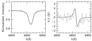
Figure 2: Flux (left) and circular polarization (right) spectra of NLTT 2219. The flux spectrum (grey) is compared to the best-fitting H$\beta$ line profile (black). The circular polarization spectrum is compared to a model polarization spectrum at $B_{l}=-97$ kG ([Kawka & Vennes (2012), Kawka & Vennes 2012]).

Spectropolarimetry has also been used to detect and measure magnetic fields in the carbon polluted DQ white dwarfs. The first DQ white dwarf that showed circular polarization was G99-37 ([Angel & Landstreet (1974), Angel & Landstreet 1974]) followed by LP 790-29 ([Liebert, et al. (1978), Liebert et al. 1978]). Estimating a magnetic field strength is still difficult for DQ white dwarfs because of their relatively broad molecular carbon bands. However, [Angel & Landstreet (1974), Angel & Landstreet (1974)] were able to obtain an estimate of the magnetic field of G99-37 using CH molecular bands, a rare feature among DQ white dwarfs. [Berdyugina, Berdyugin & Piirola (2007), Berdyugina et al. (2007)] and [Vornanen, et al. (2010), Vornanen et al. (2010)] further developed the method involving CH molecular bands to measure magnetic fields and determined a longitudinal field strength of $7.3\pm 0.3$ MG for G99-37. The same method enabled them to identify the second magnetic DQ with CH bands (GJ 841B) with a field strength $B_{l}=1.3\pm 0.5$ MG.

Currently, there are several instruments capable of spectropolarimetry. These include the FOcal Reducer and low dispersion Spectrograph (FORS2) at the European Southern Observatory ([Appenzeller, et al. (1998), Appenzeller, et al. 1998]) located at the Paranal Observatory in Chile, the Echelle SpectroPolarimetric Device for the Observation of Stars ([Donati, et al. (2006), ESPaDOnS: Donati et al. 2006)]) on the Canada-France-Hawaii Telescope (CFHT) located on Mauna Kea in Hawaii, the Intermediate-dispersion Spectrograph and Imaging System (ISIS) on the William Herschel Telescope (WHT) located on La Palma in the Canary islands, Spain and the Robert Stobie Prime Focus Imaging Spectrograph (RSS) on the South African Large Telescope near Sutherland in South Africa.

3 Population properties

To investigate the properties of magnetic white dwarfs as a population, the sample of known magnetic DA white dwarfs was cross-correlated with SDSS DR12 photometric measurements ([Alam, et al. (2015), Alam et al. 2015]) and Gaia DR2 parallax measurements ([Lindegren, et al. (2018), Lindegren et al. 2018]). The effective temperature and mass were determined by fitting the SDSS photometric measurements with synthetic magnitudes that were set to the stellar distance using Gaia parallaxes and the stellar radius $R$ by applying mass-radius relations from [Benvenuto & Althaus (1999), Benvenuto & Althaus (1999)]. Fig. 3 shows the distribution of temperature and magnetic field strength versus mass for a sample of known magnetic white dwarfs with available SDSS photometric measurements and Gaia parallaxes. The mass distribution shows that there are two peaks with the main one at $\sim 0.8\,M_{\odot}$ and the second broader one at $\sim 1.1\,M_{\odot}$. The average mass of these magnetic white dwarfs is $0.87\,M_{\odot}$, which is higher than the average mass of $0.6\,M_{\odot}$ for non-magnetic white dwarfs ([Tremblay, et al. (2019), Tremblay et al. 2019]). A higher incidence of magnetism in hot massive white dwarfs discovered by the Extreme Ultraviolet Explorer (EUVE) had already been reported by [Vennes (1999), Vennes (1999)]. There appears to be a lack of cool magnetic white dwarfs with a high mass, which is most likely due to their intrinsic faintness and a shortage of cool white dwarfs in past SDSS colour selections.

Figure 3: Mass versus temperature distribution (left) and mass versus magnetic field strength distribution (right) of magnetic DA white dwarfs from SDSS DR12.

A relationship appears to exist between the mass and magnetic field strength, with more massive white dwarfs having stronger magnetic fields, however the correlation coefficient is only 0.43 and therefore should be viewed with caution. Using population synthesis calculations under the merger scenario for the generation of fields (see Section 4), [Briggs, et al. (2015), Briggs et al. (2018)] predicted that more massive magnetic white dwarfs should have weaker fields than less massive magnetic white dwarfs, which contradicts the weak correlation observed in Fig. 3. In their simulations they show that when an asymptotic giant branch (AGB) star merges with a late stage star, it produces stronger fields than when an AGB star merges with an earlier main-sequence star. However, they also note that double degenerate mergers would not follow this trend and instead would result in more massive white dwarfs with stronger field strengths and faster rotation than magnetic white dwarfs that merged in a common envelope phase.

Using the SDSS DR2/Gaia sample of magnetic white dwarfs, we can investigate potential correlations between the cooling age of the white dwarf and the magnetic field strength and find out if there is any evidence for magnetic field decay or evolution. Fig. 4 shows no obvious correlation between the cooling age versus the magnetic field strength. The cross-correlation coefficient is only 0.14 indicating that the two properties are not correlated. [Ferrario, de Martino & Gänsicke (2015), Ferrario et al. (2015)] reached the same conclusions when they compared the magnetic field strength with the effective temperature.

Figure 4: Cooling age versus magnetic field strength distribution of the magnetic DA white dwarfs from SDSS DR12.

Many magnetic white dwarfs are faster rotators than their non-magnetic counterparts. Most rotational periods in magnetic white dwarfs were determined from photometric time series (e.g., [Brinkworth, et al. (2013), Brinkworth et al. 2013]), although some were discovered using polarimetry or spectropolarimetry. Photometric and spectropolarimetric measurements revealed that the massive, high field white dwarf RE J0317-853 (EUVE J0317-85.5) to be a very fast rotator with a period of 725 seconds ([Barstow, et al. (1995), Ferrario, et al. (1997), Vennes, et al. (2003), Barstow et al. 1995, Ferrario et al. 1997, Vennes et al. 2003]). It remained the fastest rotating white dwarf until photometric timeseries of hot DQs revealed them to have rotational periods as short as 5 minutes ([Dunlap, Barlow & Clemens (2010), Dufour, et al. (2011), e.g., Dunlap et al. 2010, Dufour et al. 2011]). Fig. 5 shows that most of the magnetic white dwarfs have rotation periods shorter than 10 hours with a distribution peaking at 2 - 3 hours. This can be compared to the rotational period distribution for non-magnetic white dwarfs determined from pulsation studies showing a mean rotation period of 35 hours ([Hermes, et al. (2017), Hermes et al. 2017]).

Figure 5: Rotational velocity versus magnetic field strength distribution for known magnetic white dwarfs for which a rotational period was measured.

Availability of photometric and astrometric data from large scale surveys has finally allowed us to better understand the properties of the magnetic white dwarf population. Detailed, case by case, spectropolarimetric investigations remain essential to understand the diverse properties of individual magnetic white dwarfs.

4 Origin of magnetic fields

The fossil field origin for the existence of magnetic white dwarfs remains a viable model because the magnetic flux of Ap/Bp stars is similar to that of magnetic white dwarfs. Assuming flux conservation ($B_{\rm WD}/B_{\rm MS}=(R_{\rm MS}/R_{\rm WD})^{2}$) the magnetic fields of Ap/Bp star can evolve into the strongest fields observed in white dwarfs ([Tout, Wickramasinghe & Ferrario (2004), Tout et al. 2004]). [Angel, Borra & Landstreet (1981), Angel et al. (1981)] compared the space density of magnetic white dwarfs to the space density of magnetic Ap/Bp stars and proposed that there is a sufficient number of Ap/Bp stars to generate all known magnetic white dwarfs. [Kawka & Vennes (2004), Kawka & Vennes (2004)] revisited this comparison and showed that if Ap/Bp stars evolve to high field magnetic white dwarfs ($B\gtrsim 10$ MG), additional progenitors are required for white dwarfs with lower field strengths. [Wickramasinghe & Ferrario (2005), Wickramasinghe & Ferrario (2005)] proposed that white dwarfs with $B\lesssim$ a few ten MG could form from main-sequence stars with $M\gtrsim 4.5\,M_{\odot}$ and low fields of $\approx 10-100$ G. However, [Aurière, et al. (2007), Aurière et al. (2007)] showed that a magnetic desert exists below 300 G for A and B type stars, which eliminates that possibility.

One of the main difficulties with the fossil field origin is that there are no known close, detached magnetic white dwarfs paired with a main-sequence star ([Liebert, et al. (2015), Liebert et al. 2015]), although thousands of close, detached but non-magnetic white dwarf plus M dwarf spectroscopic binaries have been identified in SDSS [Rebassa-Mansergas, et al. (2016), (Rebassa-Mansergas et al. 2016)].

To address this conundrum, [Tout, et al. (2008), Tout et al. (2008)] and [Wickramasinghe, Tout & Ferrario (2014), Wickramasinghe et al. (2014)] proposed that magnetic fields in isolated white dwarfs are created during a common envelope phase experienced by the progenitor close binary system. There are likely variations on the magnetic field generation model proposed by [Tout, et al. (2008), Tout et al. (2008)]. [Potter & Tout (2010), Potter & Tout (2010)] and [Wickramasinghe, Tout & Ferrario (2014), Wickramasinghe et al. (2014)] showed that a dynamo mechanism within the common envelope can generate magnetic fields with the strongest fields arising in mergers that are differentially rotating near break-up.

[Nordhaus, et al. (2011), Nordhaus et al. (2011)] also proposed a variation on the model, where the low mass star is tidally disrupted by the pre-white dwarf during the common envelope phase, resulting in the formation of an accretion disc. A dynamo is then generated in the disc creating the magnetic field which is then transferred to the degenerate core via accretion.

[García-Berro, et al. (2012), García-Berro et al. (2012)] showed that magnetic fields can also be created during the merger of two white dwarfs. When the white dwarfs merge a hot, convective and differentially rotating corona is created which produces a dynamo and, thus, the magnetic field. However, using a population synthesis of binary stars, [Briggs, et al.(2015), Briggs et al. (2015)] showed that the majority of magnetic fields in white dwarfs would have formed within a common envelope with less than 1% being formed during the merger of two white dwarfs.

[Isern, et al. (2017), Isern et al. (2017)] proposed a model where low magnetic fields ($B\lesssim 0.1$ MG) are generated by phase separation when the white dwarf begins to crystallize. They showed that when white dwarfs reach sufficiently low temperatures that the core begins crystallizing, phase separation of the main elements occurs. This leads to an unstable, convective liquid mantle on top of a solid core producing a dynamo which creates a magnetic field.

It is possible that the range of observed magnetic fields stem from several distinct processes. By studying the various classes of magnetic white dwarfs, we may be able to place constraints on the specific processes that could lead to a particular class of magnetic white dwarfs.

4.1 Double degenerate mergers

Evidence of magnetic fields being formed in double degenerate mergers has been found in common proper motion binaries. EUVE J0317-85.5 is a hot ($T_{\rm eff}=33\,000$ K), strongly magnetic ($B=450$ MG) and massive white dwarf ($M=1.3\,M_{\odot}$) in common proper motion with the non-magnetic white dwarf LB 9802 ([Barstow, et al. (1995), Ferrario, et al. (1997), Vennes, et al. (2003), Barstow et al. 1995, Ferrario et al. 1997, Vennes et al. 2003]). EUVE J0317-85.5 being significantly more massive than LB 9802 would have had a more massive main-sequence progenitor and therefore it should have a much longer cooling age compared to LB 9802. However, EUVE J0317-85.5 is much hotter than LB 9802, and therefore its cooling age is also shorter. This strongly suggests that EUVE J0317-85.5 is the result of a merger ([Ferrario, et al. (1997), Ferrario et al. 1997]). Another possible example is the common proper motion binary SDSS J150746.49+521002.1 plus SDSS J150746.80+520958.0. SDSS J1507+5209 is magnetic and more massive than SDSS J1507+5210, however their effective temperatures are similar ([Dobbie, et al. (2012), Dobbie et al. 2012]). Since they are in a common proper motion binary, their total ages should be the same, however the total age of the magnetic white dwarf is much shorter than the total age of the non-magnetic companion. Therefore SDSS J1507+5209 is most likely the product of a merger and thus the original system was a triple system.

A small number of common proper motion binaries provide evidence to support that some magnetic fields in white dwarfs are formed through mergers. The key property is the discrepancy in the total ages of the magnetic white dwarf and non-magnetic white dwarf if single star evolution is assumed for both stars.

Spectroscopic follow-up of newly identified common proper motion white dwarf pairs may add additional cases and shed more light on the origin of magnetic fields.

4.2 Incidence of magnetism

Table 2: Incidence of magnetism among different classes of white dwarfs.

Spectral Type	Prototype	Reference	Fraction (%)	Reference
DAH	Grw+70∘8247	[kem1970, Kemp et al. (1970)]	$4\pm 1.4$	[Schmidt & Smith (1995), Schmidt & Smith (1995)]
DAZH (cool)	G77$-$50	[Farihi et al. (2011), Farihi et al. (2011)]	$\sim 50$	[Kawka, et al. (2019), Kawka et al. (2019)]
DBH	GD229	[Swedlund, et al. (1974), Swedlund et al. (1974)]	$\sim 1.5$	[Kawka (2018), Kawka (2018)]
DCP	G195$-$19	[Angel & Landstreet (1971), Angel & Landstreet (1971)]	$\sim 5$	[Putney (1997), Putney (1997)]
DZH (cool)	LHS2534	[Reid, Liebert & Schmidt (2001), Reid et al. (2001)]	$21.6\pm 3.3$	[Hollands (2017), Hollands (2017)]
DQH (hot)	SDSS J1337$+$0026	[Dufour, et al. (2007), Dufour et al. (2007)]	$\sim 70$	[Dufour, et al. (2013), Dufour et al. (2013)]
DQH (cool)	G99$-$37	[Landstreet & Angel (1971), Landstreet & Angel (1971)]	$\sim 4$	[Vornanen, Berdyugina & Berdyugin (2013), Vornanen et al. (2013)]

The incidence of magnetism varies between different spectral classes, but it is also affected by the population sampling criteria. Taking the population of magnetic white dwarfs as a whole, then in magnitude limited surveys such as those of Palomar-Green or SDSS ([Schmidt & Smith (1995), Kepler, et al.(2013), Schmidt & Smith 1995, Kepler et al. 2013]) the incidence is as low as $\sim 5$%, while in volume limited surveys, the incidence is much higher at $13-20$% ([Kawka, et al. (2007), Kawka et al. 2007]). Table 2 lists the many classes of magnetic white dwarfs including the individual prototypes and the incidence within specific spectral classes.

4.2.1 Common proper motion binaries

It was already mentioned that there are no close, detached magnetic white dwarfs paired with a main sequence star, however there are a few magnetic white dwarfs in common proper motion with a main sequence star. In these systems the stars are assumed to have been born at the same time and remain distant enough from each other to avoid interaction and thereby follow single star evolution. An examination of the incidence of magnetic white dwarfs in such systems within the Solar neighbourhood ($d<20$ pc) reveals that magnetic white dwarfs in wide binaries are not that rare. [Holberg, et al. (2013), Holberg et al. (2013)] identified 11 so-called Sirius-like systems within 20 pc of the Sun. These are systems where the white dwarf is paired with a main sequence star with a spectral type of K or earlier. Of these 11 binary systems, one has a magnetic white dwarf: WD 1009$-$184 is a cool, polluted helium rich white dwarf with a weak surface averaged field of $\approx 300$ kG ([Bagnulo & Landstreet (2019), Bagnulo & Landstreet 2019]). Therefore, this sets an incidence of $\sim 9$%, comparable to the incidence of single magnetic white dwarfs. More recently, [Hollands, et al. (2018), Hollands et al. (2018)] revisited the 20 pc sample with Gaia and identified a total of 30 white dwarfs that are in a wide binary system with a main sequence companion (including M dwarfs) and 3 of these are magnetic. These include WD 1009$-$184, along with the cool DA WD2150$+$591 ([Landstreet & Bagnulo (2019), Landstreet & Bagnulo 2019]) and the cool DQ WD2153$-$512 ([Vornanen, et al. (2010), Vornanen et al. 2010]). This corresponds to an incidence of $\sim 10$%. If we exclude systems that are likely to interact or have already interacted, then this incidence would be higher. The formation of magnetic fields in white dwarfs that are in wide binaries can be assumed to follow the same paths as those followed by isolated magnetic white dwarfs.

4.2.2 Polluted white dwarfs

Magnetic fields have been detected in all spectral classes of white dwarfs. Most of the known magnetic white dwarfs have hydrogen-rich atmospheres, similar to non-magnetic white dwarfs. Some spectral classes of white dwarfs display significantly higher incidence of magnetism than the general white dwarf population. Cool, polluted white dwarfs show an enhanced incidence of magnetism. [Kawka & Vennes (2014), Kawka & Vennes (2014)] and [Kawka, et al. (2019), Kawka et al. (2019)] showed that $\approx 50\%$ of cool ($T_{\rm eff}<6000$ K), polluted hydrogen-rich DAZ white dwarfs are magnetic with field strengths below 1 MG. Similarly, [Hollands, et al. (2015), Hollands et al. (2015)] and [Hollands (2017), Hollands (2017)] showed that $21.6\pm 3.3$% of cool ($T_{\rm eff}<8000$ K) polluted helium-rich DZ white dwarfs are magnetic with field strengths ranging from $\approx 0.3$ MG up to $\approx 30$ MG. Only two DAZ white dwarfs with an effective temperature above 6000 K have magnetic fields, NLTT 53908 which is only slightly warmer at 6250 K ([Kawka & Vennes (2014), Kawka & Vennes 2014]) and WD 2105-820 which is much hotter at $T_{\rm eff}=10800$ K ([Landstreet, et al. (2012), Landstreet et al. 2012]). In the case of DZ white dwarfs, [Hollands (2017), Hollands (2017)] found that there are no known magnetic DZ white dwarfs warmer than 8000 K. The lack of warmer counterparts to the magnetic, polluted white dwarfs provides constraints on the origin of the magnetic field in these stars. Some of these possibilities are discussed below.

One possible scenario which may explain the presence of magnetic fields in this particular class involves a gaseous planet colliding with an older white dwarf creating differential rotation which would generate a relatively weak magnetic field ([Farihi et al. (2011), Kawka, et al. (2019), Farihi et al. 2011, Kawka et al. 2019]). The time-scale for a post main sequence planetary system to dynamically stabilize is relatively short at about 100 Myr ([deb2002, Debes & Sigurdsson 2002]). Therefore, at the old ages encountered in cool DAZs and DZs ($>1$ Gyr) a destabilizing agent is required to create a planetary or asteroidal debris disc causing atmospheric pollution and contributing to the creation of a magnetic field. [Farihi et al. (2011), Farihi et al. (2011)] proposed that planets and asteroids could be destabilized by a close encounter with another star. These cool white dwarfs have been orbiting the Galaxy for billions of years and [Farihi et al. (2011), Farihi et al. (2011)] estimated that a stellar encounter has a 50% probability of occurring every 0.5 Gyr. Therefore, the older the white dwarf, the more likely it will encounter a star that is close enough to perturb the orbit of the outer planets. If one of these planets is a gaseous type then this would create the magnetic field while the perturbed rocky planets and asteroids would pollute the white dwarf. The pairing of these events would explain the dual nature of polluted, magnetic white dwarfs.

[Hollands (2017), Hollands (2017)] suggested that cool, polluted and magnetic white dwarfs could have been generated in the cores of giant stars following [Kissin & Thompson (2015), Kissin & Thomson (2015)]. In this scenario, a dynamo is generated within the giant core during the shell burning phases. They showed that angular momentum pumped inward in combination with the absorption of a planet or a binary companion could generate a dynamo at the boundary between the radiative and convective envelopes. This could create magnetic fields of up to about $10^{7}$ G. However this magnetic field could remain buried below a non-magnetized envelope for up to about 1 - 2 Gyr. Since the creation of the magnetic field is aided by the engulfment of a planet, it is likely that other planets or asteroids could survive and with time migrate closer toward the white dwarf and be accreted polluting the white dwarf atmosphere.

4.2.3 Hot DQ white dwarfs

The class of hot DQs shows the highest incidence of magnetism among the various classes of white dwarfs. Approximately 70% of hot DQs are magnetic ([Dufour, et al. (2013), Dufour et al. 2013]). Hot DQs have temperatures ranging from 18 000 K up to 24 000 K and have an atmosphere dominated by carbon ([Dufour, et al. (2008), Dufour et al. 2008]). [Coutu, et al. (2019), Coutu et al (2019)] showed that they are all massive ($0.8-1.2$ M_⊙) and about half of these stars have been found to be photometrically variable with periods ranging from about 5 minutes up to 2.1 days. These variations have been attributed to the rotation of the white dwarfs ([Dunlap & Clemens (2015), Williams, et al. (2016), Dunlap & Clemens 2015, Williams et al. 2016]). These properties point toward hot DQ white dwarfs being the outcome of mergers of white dwarfs. [Coutu, et al. (2019), Coutu et al. (2019)] showed that the hot DQ sequence extends toward lower temperatures. These cooler objects are also massive and they can be distinguished from normal mass ($\sim 0.6$ M_⊙) DQ white dwarfs by having a higher carbon abundance. [Coutu, et al. (2019), Coutu et al. (2019)] also showed that the distribution of transverse velocities of these objects is larger than for other classes of objects with similar temperatures, suggesting that they must come from an older population. If these massive DQs formed in a double degenerate merger, this would provide the necessary delay to make these stars appear younger than they really are. One star where we clearly see a discrepancy between the total age assuming single star evolution and the age based on kinematics is LP 93-21, which is a massive DQ with halo like orbit ([Kawka, Vennes & Ferrario (2020), Kawka et al. 2020]) and is thus highly unlikely to be the unburnt remnant of a subluminous Type Ia supernova explosion ([Vennes, et al. (2017), e.g., Vennes et al. 2017]) as proposed by [Ruffini & Casey (2019), Ruffini & Casey (2019)]. It is likely that the majority of these cooler massive DQs will also harbour a magnetic field and be fast rotators. The number of these massive DQs is small compared to other classes of white dwarfs, however it is in agreement with the conclusion of [Briggs, et al.(2015), Briggs et al. (2015)] who predicted that less than about one in four hundred mergers involve double degenerate mergers.

The different properties of the various classes of magnetic white dwarfs, along with their respective incidences of magnetism allows links to be established with potential formation scenarios.

5 Structure of magnetic atmospheres

Magnetic fields have the potential to affect the transport of energy within a stellar atmosphere, and therefore the atmospheric structure as well. Field variations across the stellar surface add more complexities to this problem.

5.1 Convective energy transport

As white dwarfs cool, they develop convection zones with a depth increasing with age ([Fontaine, et al. (2013), Fontaine et al. 2013]). White dwarfs with hydrogen-rich atmospheres begin to develop a convection zone at about 14 000 K, whereas white dwarfs with helium-rich atmospheres develop convective zones much earlier at about 30 000 K. As white dwarfs cool, these convection zones become the main energy transport mechanism, however it is possible that if a magnetic field is present, this transport of energy can be affected. Suppression of convection by magnetic fields was first investigated by [D’Antona & Mazzitelli (1975), D’Antona & Mazzitelli (1975)]. Furthermore, [Wickramasinghe & Martin (1986), Wickramasinghe & Martin (1986)] assumed that magnetic fields can provide resistance to large scale motions and therefore convective energy transport was suppressed in their atmospheric models.

Recently, [Valyavin, et al. (2014), Valyavin et al. (2014)] revisited the idea that magnetic fields can suppress convection to explain the higher incidence of magnetism among cool white dwarfs ([Liebert & Sion (1979), Valyavin & Fabrika (1999), Liebert & Sion 1979, Valyavin & Fabrika 1999]). They argued that suppression of convection causes a slow down in white dwarf cooling for white dwarfs below 12 000 to 14 000 K. [Tremblay, et al. (2015), Tremblay et al. (2015)] conducted radiation magnetohydrodynamic simulations and showed that convection can be inhibited in a white dwarf atmosphere by magnetic fields as low as 50 kG, but that the cooling age is not affected until the convective zone couples with the degenerate core. This occurs at about 6000 K for higher mass white dwarfs ($M\sim 1\,M_{\odot}$) and at lower temperatures for lower mass white dwarfs.

Empirical support for suppression of convection was provided by [Bédard, Bergeron & Fontaine (2017), Bédard, Bergeron & Fontaine (2017)] and [Gentile Fusillo, et al. (2018), Gentile Fusillo et al. (2018)] using the weakly magnetic white dwarf WD 2105$-$820 ([Landstreet, et al. (2012), Landstreet et al. 2012]). The effective temperature of WD 2105$-$820 is about 10 000 K and, therefore, it is cool enough to develop a shallow convective zone. [Bédard, Bergeron & Fontaine (2017), Bédard, et al. (2017)] showed that using radiative models they were able to match the photometrically and spectroscopically derived effective temperatures, as well as match the spectroscopically determined distance with the measured parallax. However, convective models showed discrepancies between the spectroscopically and photometrically determined temperatures, as well as the distance obtained from the spectroscopic solutions and the measured parallax. Non-magnetic white dwarfs with similar temperature to WD 2105$-$820 show good agreement between spectroscopically and photometrically determined temperatures when using convective models. Additional support for the inhibition of convection was presented by [Gentile Fusillo, et al. (2018), Gentile Fusillo et al. (2018)], who showed that consistent results were obtained from fitting ultraviolet and optical spectra when using purely radiative models, whilst fitting with convective models resulted in inconsistent results. Again, non-magnetic white dwarfs with similar temperatures show consistent results when convective models are used.

Cooler magnetic white dwarfs have deeper and thicker convection zones. [Kawka, et al. (2019), Kawka et al. (2019)] analyzed the cool ($\approx 5200$ K), magnetic white dwarf NLTT 7547 using convective and radiative models. Their analysis showed that the convective models provide a better fit to the Balmer lines compared to radiative models. They also showed that by suppressing convection in the model atmospheres, the temperature gradient steepens sharply at larger optical depths and higher pressure. The model atmospheres also show a downturn in the density at higher pressure which would give rise to a Rayleigh-Taylor instability. They concluded that convective models are preferred in cool and magnetic white dwarfs. [Bédard, Bergeron & Fontaine (2017), Bédard et al. (2017)] also analyzed a sample of cool (6600 - 8510 K) and magnetic white dwarfs and showed that in these white dwarfs, consistent results between spectroscopic and photometric solutions, as well as distances inferred from spectroscopy and parallax were achieved with convective models. As a result, they concluded that it may become more difficult to suppress convection in cooler white dwarfs where convective energy transport becomes more important.

A small number of cool, average mass and magnetic DQs are known ([Schmidt, et al. (1999), Vornanen, et al. (2010), e.g., Schmidt et al. 1999, Vornanen et al. 2010]). The carbon in the atmospheres of these DQs is dredged up from the core by the deep convection zone ([Pelletier, et al. (1986), Pelletier et al. 1986]). If convection is suppressed by the magnetic field, then we should not find any magnetic DQ white dwarfs since there is no convective motion to bring up the carbon to the surface. There are two possibilities to explain the existence of these cool and magnetic DQs. The first is that the carbon is not dredged up but it has been present in the atmosphere from the outset and as such they could be the descendants of hot DQs. In this case, they should also be massive. The two prototypical magnetic DQs, LHS2229 and LP 790-29, have $T_{\rm eff}<5000$ K and $M\lesssim 0.7\,M_{\odot}$ ([Blouin, et al. (2019), Blouin et al. 2019]). They are also not known to vary rapidly. The second explanation is the same as for the cool magnetic DA white dwarfs, that is the convection zone is too deep and therefore the magnetic field cannot suppress it.

5.2 Magnetic field structure

The magnetic field structure in a white dwarf can provide clues to how the magnetic field was created. Complex magnetic fields are predicted for white dwarfs that formed in a merger ([García-Berro, et al. (2012), García-Berro, et al. 2012]). Simpler fields that are approximately dipolar maybe an attribute of white dwarfs that are descendants of Ap or Bp stars ([Braithwaite & Spruit (2004), Braithwaite & Spruit 2004]). When modelling the magnetic field geometry in white dwarfs, a centred or offset dipole is often assumed. However, rotating white dwarfs provide the means to study the field structure and reveal a diversity in the field geometry. Depending on the magnetic field structure the Zeeman splitted lines may vary as a function of the rotational phase and reveal how the magnetic field strength varies on the white dwarf surface. In addition to measuring the strength of the magnetic field, circular and linear polarization can provide the direction of the magnetic field. With a series of circular polarization spectra covering the rotation period of 0.243 days, [Landstreet, et al. (2017), Landstreet et al. (2017)] showed that WD 2047$+$372 can be modelled by a simple dipole with a weak field of $91.8\pm 0.8$ kG. However, their analysis of WD 2359$-$434 revealed a more complex field structure, which required a combination of a dipolar field and a non-aligned quadrupolar field.

Detailed modelling of rotating white dwarfs with stronger fields has resulted in even more complex structures. The high field, massive and hot white dwarf EUVE J0317$-$855 has a field of 185 MG with a magnetic spot of 425 MG ([Burleigh, Jordan & Schweizer (1999), Vennes, et al. (2003), Burleigh et al. 1999, Vennes et al. 2003]). Another white dwarf with a magnetic spot is WD 1953-011 ([Maxted, et al. (2000), Valyavin, et al. (2008), Maxted et al. 2000, Valyavin et al. 2008]) which was revealed over its rotational period of 1.4418 days ([Brinkworth, et al. (2005), Brinkworth et al. 2005]). [Euchner, et al. (2006), Euchner et al. (2006)] used Zeeman tomography to show that the magnetic field of PG 1015$+$014 is a combination of three individually offset non-aligned dipoles.

Our study of the structure of magnetic white dwarf atmospheres offers computational challenges. Complete suppression of the convection zone appears unlikely at lower temperatures. Complex surface field distributions are observed in several white dwarfs but such observations are challenging and impractical in most cases.

6 Summary

With the growth of large scale photometric, spectroscopic and astrometric surveys we have been able to study the magnetic white dwarf population as a whole in greater detail. The growing sample of white dwarfs has revealed that the incidence of magnetism varies across the spectral classes, with the class of hot DQs showing the highest incidence at about 70%. There is evidence that these objects are a result of double degenerate mergers, which is one of the proposed scenarios for the creation of magnetic fields.

There are several proposed scenarios for the creation of magnetic fields in white dwarfs, with the merging scenario being favoured, although many challenges remain. It is also likely that magnetic fields in white dwarfs may be created by several distinct processes.

The magnetic field structure across the surface can be complex. We have some observational evidence that shows that the white dwarf atmospheric structure is affected by the presence of a magnetic field, such as the suppression of convection. This provides computational challenges in modelling white dwarf atmospheres in the presence of complex magnetic fields.

Acknowledgements

AK thanks S. Vennes, L. Ferrario and D.T. Wickramasinghe for stimulating discussions and the Science Organizing Committee for the kind invitation to present this review. The International Centre for Radio Astronomy Research is a joint venture between Curtin University and the University of Western Australia, funded by the state government of Western Australia and the joint venture partners.

References

- [Alam, et al. (2015)] Alam, S., et al. 2015, ApJS, 219, 12
- [Al-Hujaj & Schmelcher (2003)] Al-Hujaj, O.-A., Schmelcher, P. 2003, PhRvA, 68, 053403
- [Angel, Borra & Landstreet (1981)] Angel, J. R. P., Borra, E. F., Landstreet, J. D. 1981, ApJS, 45, 457
- [Angel & Landstreet (1971)] Angel, J. R. P., Landstreet, J. D. 1971, ApJ Letters, 164, L15
- [Angel & Landstreet (1974)] Angel, J. R. P., Landstreet, J. D. 1974, ApJ, 191, 457
- [Appenzeller, et al. (1998)] Appenzeller, I., et al. 1998, Msngr, 94, 1
- [Aurière, et al. (2007)] Aurière M., et al. 2007, A&A, 475, 1053
- [Babcock (1947)] Babcock, H. W. 1947, ApJ, 105 105
- [Bagnulo & Landstreet (2019)] Bagnulo, S., Landstreet, J. D. 2019, A&A, 630, A65
- [Barstow, et al. (1995)] Barstow, M. A., Jordan, S., O’Donoghue, D., Burleigh, M. R., Napiwotzki, R., Harrop-Allin, M. K. 1995, MNRAS, 277, 971
- [Becken & Schmelcher (2001)] Becken, W., Schmelcher, P. 2001, PhRvA, 63, 053412
- [Bédard, Bergeron & Fontaine (2017)] Bédard, A., Bergeron, P., Fontaine, G. 2017, ApJ, 848, 11
- [Benvenuto & Althaus (1999)] Benvenuto, O. G., Althaus, L. G. 1999, MNRAS, 303, 30
- [Berdyugina, Berdyugin & Piirola (2007)] Berdyugina, S. V., Berdyugin, A. V., Piirola, V. 2007, PhRvL, 99, 091101
- [Blackett (1947)] Blackett, P. M. S. 1947, Nature, 159, 658
- [Blouin, et al. (2019)] Blouin, S., Dufour, P., Thibeault, C., Allard, N. F. 2019, ApJ, 878, 63
- [Braithwaite & Spruit (2004)] Braithwaite, J., Spruit, H. C. 2004, Nature, 431, 819
- [Briggs, et al.(2015)] Briggs, G. P., Ferrario, L., Tout, C. A., Wickramasinghe, D. T., Hurley, J. R. 2015, MNRAS, 447, 1713
- [Briggs, et al. (2015)] Briggs, G. P., Ferrario, L., Tout, C. A., Wickramasinghe, D. T. 2018, MNRAS, 478, 899
- [Brinkworth, et al. (2013)] Brinkworth, C. S., Burleigh, M. R., Lawrie, K., Marsh, T. R., Knigge, C. 2013, ApJ, 773, 47
- [Brinkworth, et al. (2005)] Brinkworth, C. S., Marsh, T. R., Morales-Rueda, L., Maxted, P. F. L., Burleigh, M. R., Good, S. A. 2005, MNRAS, 357, 333
- [Burleigh, Jordan & Schweizer (1999)] Burleigh, M. R., Jordan, S., Schweizer, W. 1999, ApJ Letters, 510, L37
- [Coutu, et al. (2019)] Coutu, S., Dufour, P., Bergeron, P., Blouin, S., Loranger, E., Allard, N. F., Dunlap, B. H. 2019, ApJ, 885, 74
- [D’Antona & Mazzitelli (1975)] D’Antona, F., Mazzitelli, I. 1975, A&A, 42, 127
- [Dobbie, et al. (2012)] Dobbie, P. D., et al. 2012, MNRAS, 421, 202
- [Donati, et al. (2006)] Donati, J.-F., Catala, C., Landstreet, J. D., Petit, P. 2006, ASP Conf. Ser. Vol. 358, 362
- [Dufour, et al. (2007)] Dufour, P., Liebert, J., Fontaine, G., Behara, N. 2007, Nature, 450, 522
- [Dufour, et al. (2011)] Dufour, P., Béland, S., Fontaine, G., Chayer, P., Bergeron, P. 2011, ApJ Letters, 733, L19
- [Dufour, et al. (2008)] Dufour, P., Fontaine, G., Liebert, J., Schmidt, G. D., Behara, N. 2008, ApJ, 683, 978
- [Dufour, et al. (2013)] Dufour, P., Vornanen, T., Bergeron, P., Fontaine, G., Berdyugin, A. 2013, ASP Conf. Ser. Vol. 469, 167
- [Dunlap, Barlow & Clemens (2010)] Dunlap, B. H., Barlow, B. N., Clemens, J. C. 2010, ApJ Letters, 720, L159
- [Dunlap & Clemens (2015)] Dunlap, B. H., Clemens, J. C. 2015, ASP Conf. Ser., Vol. 493, 547
- [Euchner, et al. (2006)] Euchner, F., Jordan, S., Beuermann, K., Reinsch, K., Gänsicke, B. T. 2006, A&A, 451, 671
- [Farihi et al. (2011)] Farihi, J., Dufour, P., Napiwotzki, R., Koester, D. 2011, MNRAS, 413, 2559
- [Ferrario, de Martino & Gänsicke (2015)] Ferrario, L., de Martino, D., Gänsicke, B. T. 2015, SSRv, 191, 111
- [Ferrario, et al. (1997)] Ferrario, L., Vennes, S., Wickramasinghe, D. T., Bailey, J. A., Christian, D. J. 1997, MNRAS, 292, 205
- [Ferrario, Wickramasinghe & Kawka (2019)] Ferrario, L., Wickramasinghe, D., Kawka, A. 2019, AdSpR, in press
- [Fontaine, et al. (2013)] Fontaine, G., Brassard, P., Charpinet, S., Randall, S. K., Van Grootel, V. 2013, ASP Conf. Ser. Vol. 479, 211