Constructing a subgradient from directional derivatives for functions of two variables

Abstract

For any scalar-valued bivariate function that is locally Lipschitz continuous and directionally differentiable, it is shown that a subgradient may always be constructed from the function’s directional derivatives in the four compass directions, arranged in a so-called “compass difference”. When the original function is nonconvex, the obtained subgradient is an element of Clarke’s generalized gradient, but the result appears to be novel even for convex functions. The function is not required to be represented in any particular form, and no further assumptions are required, though the result is strengthened when the function is additionally L-smooth in the sense of Nesterov. For certain optimal-value functions and certain parametric solutions of differential equation systems, these new results appear to provide the only known way to compute a subgradient. These results also imply that centered finite differences will converge to a subgradient for bivariate nonsmooth functions. As a dual result, we find that any compact convex set in two dimensions contains the midpoint of its interval hull. Examples are included for illustration, and it is demonstrated that these results do not extend directly to functions of more than two variables or sets in higher dimensions.

Keywords: subgradients, directional derivatives, support functions, Clarke’s generalized gradient, interval hull

1 Introduction

Subgradient methods [40, 2] and bundle methods [26, 28, 29, 2] for nonsmooth optimization typically use a subgradient at each iteration to provide local sensitivity information that is ultimately useful enough to infer descent. For convex problems, these subgradients are elements of the convex subdifferential; for nonconvex problems, the subgradients must typically be elements of either Clarke’s generalized gradient [6] or other established generalized subdifferentials [32, 31, 27]. Evaluating a subgradient directly, however, may be a challenging task; this difficulty has motivated the development of numerous subdifferential approximations [2, 11, 34].

Nevertheless, there are several settings in which evaluating directional derivatives is much simpler than evaluating a subgradient using established methods. For finite compositions of simple smooth and nonsmooth functions, directional derivatives may be evaluated efficiently [12] by extending the standard forward/tangent mode of algorithmic differentiation [13], while extensions to efficient subgradient evaluation methods require more care [24, 21]. Directional derivatives of implicit functions and inverse functions may be obtained by solving auxiliary equation systems [39], whereas subgradient results in this setting assume either special structure [39, 25] or a series of recursive equation-solves [25]. For solutions of parametric ordinary differential equations (ODEs) with nonsmooth right-hand sides, directional derivatives may be evaluated by solving an auxiliary ODE system [34, Theorem 7] using a standard ODE solver, whereas the only general method for subgradient evaluation involves solving a series of ODEs punctuated by discrete jumps that must be handled carefully [23, 19]. In parametric optimization, Danskin’s classical result [8, 17] describes directional derivatives for optimal-value functions as the solutions of related optimization problems in a general setting, while subgradient results such as [43, Theorem 5.1] tend to additionally require unique solutions for the embedded optimization problem.

Moreover, directional derivatives and subdifferentials of convex functions are essentially duals [15]. Hence, this article examines the question of whether, given a directional-derivative evaluation oracle for a function and little else, this oracle may be used to compute a subgradient at each iteration of a typical nonsmooth optimization method. This is clearly true for univariate functions, for example; in this case, the entire subdifferential may be constructed from directional derivatives in the positive and negative directions.

To address this question, this article defines a function’s compass differences to be vectors obtained by arranging directional derivatives in the coordinate directions and negative coordinate directions in a certain way. Thus, for a bivariate function, a compass difference involves directional derivatives in the four compass directions. For a bivariate function that is locally Lipschitz continuous and directionally differentiable, it is shown that the compass difference at any domain point is a subgradient, with this subgradient understood to be an element of Clarke’s generalized gradient in the nonconvex case. Surprisingly, while this result is simple to state, it appears to be previously unknown even for convex functions, and does not require any additional assumptions. It is also shown that this result does not extend directly to functions of more than two variables. As a related result, this article shows that a compact convex set in $\mathbb{R}^{2}$ must always contain the midpoint of its interval hull, though this does not extend directly to sets in $\mathbb{R}^{n}$ for $n>2$. Hence, four calls to a directional-derivative evaluation oracle are sufficient to compute a subgradient for a nonsmooth bivariate function, and centered finite differences for these functions are useful approximations of a subgradient. In several cases, the approach of this article appears to be the only way known thus far to evaluate a subgradient correctly.

Audet and Hare [1] studied a similar problem involving the similar setup, in the field of geometric probing [41]. Unlike our work, Audet and Hare additionally assume that: (a) their oracle $\mathsf{D}$ is convex (as a set’s support function), (b) the bivariate function’s regular subdifferential is polyhedral, and (c) the oracle $\mathsf{D}$ evaluates the function’s directional derivative. These assumptions are evidently satisfied, for example, by any function that is both convex and piecewise-differentiable in the sense of Scholtes [39]. Under these assumptions, Audet and Hare present a method to use finitely many directional derivative evaluations to construct the whole regular subdifferential at a given domain point. This method proceeds by deducing each vertex of the subdifferential, and depends heavily on the assumption of subdifferential polyhedrality; its complexity scales linearly with the number of subdifferential vertices. It is readily verified, for example, that their Algorithm 1 will run forever without locating any subgradients when applied to the convex Euclidean norm function:

$$f:\mathbb{R}^{2}\to\mathbb{R}:x\mapsto\sqrt{x_{1}^{2}+x_{2}^{2}}$$

at $x=0$. Indeed, their algorithm is not intended to work in this case. Unlike the work of [1], we do not assume that subdifferentials are polyhedral, do not require the subdifferential’s support function to be available in the nonconvex case, and do not assume directional derivatives to be convex with respect to direction. Our goal is only to identify one subgradient rather than a whole subdifferential; characterizing a whole subdifferential in closed form may be difficult or impossible when we do not know a priori that it is polyhedral. As mentioned above, in the nonconvex case, we evaluate an element of Clarke’s generalized gradient [6] instead of a subgradient.

The remainder of this article is structured as follows. Section 2 summarizes relevant established constructions in nonsmooth analysis, Section 3 defines compass differences in terms of directional derivatives and shows that they are valid subgradients, and Section 4 presents several examples for illustration.

2 Mathematical background

The Euclidean norm $\|\cdot\|$ and inner product $\langle\cdot,\cdot\rangle$ are used throughout this article. The ${i}^{\text{th}}$ unit coordinate vector in $\mathbb{R}^{n}$ is denoted as ${e}_{(i)}$, and components of vectors are indicated using subscripts, e.g. $x_{i}\coloneqq\langle{e}_{(i)},x\rangle$. The convex hull and the closure of a set $S\subset\mathbb{R}^{n}$ are denoted as $\mathrm{conv}\,S$ and $\mathrm{cl}\,S$, respectively.

2.1 Directional derivatives and convex subgradients

Definition 2.1.

Consider an open set $X\subset\mathbb{R}^{n}$ and a function $f:X\to\mathbb{R}$. The following limit, if it exists, is the (one-sided) directional derivative of $f$ at $x\in X$ in the direction $d\in\mathbb{R}^{n}$:

$${f}^{\prime}(x;d)\coloneqq\lim_{t\to{0}^{+}}\frac{f(x+td)-f(x)}{t}.$$

If ${f}^{\prime}(x;d)$ exists in $\mathbb{R}$ for each $d\in\mathbb{R}^{n}$, then $f$ is directionally differentiable at $x$.

This article primarily considers situations where directional derivatives are available via a black-box oracle. For example, this oracle could represent symbolic calculation, the situation-specific directional derivatives described in Section 1, algorithmic differentiation [13], or even finite difference approximation if some error is tolerable.

The primary goal of this article is to use directional derivatives to evaluate a subgradient, defined for convex functions as follows, and generalized to nonconvex functions as in Section 2.2 below. Individual subgradients are used at each iteration of subgradient methods for convex minimization [40] and bundle methods for nonconvex minimization [16]. They are also used to build useful affine outer approximations for nonconvex sets [38, 22]. In each of these applications, only a single subgradient is needed at each visited domain point.

Definition 2.2.

Given a convex set $X\subset\mathbb{R}^{n}$ and a convex function $f:X\to\mathbb{R}$, $s\in\mathbb{R}^{n}$ is a subgradient of $f$ at $x\in X$ if

(1) $$f(y)\geq f(x)+\langle s,y-x\rangle,\qquad\forall y\in X.$$

The set of all subgradients of $f$ at $x$ is the (convex) subdifferential $\partial f(x)$.

In this definition, if $X$ is open, then $\partial f(x)$ is convex, compact, and nonempty [15]. The directional derivative and subdifferentials of $f$ at $x$ are related as follows [15]. For each $d\in\mathbb{R}^{n}$,

(2) $${f}^{\prime}(x;d)=\max\{\langle s,d\rangle:\,\,s\in\partial f(x)\}\quad\text{and}\quad\partial f(x)=\{s\in\mathbb{R}^{n}:{f}^{\prime}(x;d)\geq\langle s,d\rangle,\,\,\forall d\in\mathbb{R}^{n}\}.$$

Thus, the subdifferential characterizes the local behavior of convex functions via (2), and characterizes the global behavior of convex functions via (1). Moreover, (2) shows that directional derivatives and subgradients of convex functions are essentially duals of each other.

2.2 Nonsmooth analysis

The following constructions by Clarke [6] extend certain subgradient properties to nonconvex functions, and are used in methods for equation-solving [36, 10] and optimization [40, 26, 30].

Definition 2.3.

Consider an open set $X\subset\mathbb{R}^{n}$ and a locally Lipschitz continuous function $f:X\to\mathbb{R}$. The (Clarke–)generalized directional derivative of $f$ at $x\in X$ in the direction $d\in\mathbb{R}^{n}$ is:

$$f^{\circ}(x;d)\coloneqq\limsup_{\begin{subarray}{c}y\to x\\ t\to{0}^{+}\end{subarray}}\frac{f(y+td)-f(y)}{t}.$$

Clarke’s generalized gradient of $f$ at $x$ is then:

$$\partial f(x)\coloneqq\{s\in\mathbb{R}^{n}:f^{\circ}(x;d)\geq\langle s,d\rangle,\quad\forall d\in\mathbb{R}^{n}\}.$$

Elements of Clarke’s generalized gradient will be called Clarke subgradients.

With $f$ as in the above definition, and for any $x\in X$, $\partial f(x)$ is guaranteed to be nonempty, convex, and compact in $\mathbb{R}^{n}$. As suggested by its notation, Clarke’s generalized gradient does indeed coincide with the convex subdifferential when $f$ is convex [6]. When $f$ is nonconvex, (2) is no longer guaranteed to hold with Clarke’s generalized gradient in place of the convex subdifferential. The following result for univariate functions is easily demonstrated, and is summarized in [1].

Proposition 2.4.

Consider an open set $X\subset\mathbb{R}$ and a univariate function $f:X\to\mathbb{R}$ that is locally Lipschitz continuous and directionally differentiable. For each $x\in X$,

(3) $$\partial f(x)=\mathrm{conv}\,\{{f}^{\prime}(x;1),-{f}^{\prime}(x;-1)\}.$$

Hence, one call to an oracle that evaluates directional derivatives is sufficient to obtain a single Clarke subgradient for such a univariate function $f$. It will be shown in this article that, for bivariate functions $f:\mathbb{R}^{2}\to\mathbb{R}$ that are locally Lipcshitz continuous and directionally differentiable, four directional derivative evaluations are sufficient to evaluate a single Clarke subgradient.

The following definition by Nesterov [32] will be used to specialize this result in a useful way. Nesterov’s definition is based on repeated directional differentiation, and permits certain extensions of calculus rules for smooth functions to nonsmooth functions.

Definition 2.5.

Consider an open set $X\subset\mathbb{R}^{n}$ and a locally Lipschitz continuous function $f:X\to\mathbb{R}$. The function $f$ is lexicographically (L–)smooth at $x\in X$ if the following conditions are satisfied:

• $f$ is directionally differentiable at $x$,

• with $f^{(0)}\coloneqq{f}^{\prime}(x;\cdot)$, for any collection of vectors $m_{(1)},\ldots,m_{(n)}\in\mathbb{R}^{n}$, the following inductive sequence of higher-order directional derivatives is well-defined:

  $$f^{(k)}\coloneqq{[f^{(k-1)}]}^{\prime}(m_{(k)};\cdot),\qquad\text{for each }k\in\{1,2,\ldots,n\}.$$

If these vectors $m_{(i)}$ are linearly independent, then $f^{(n)}$ is linear, and its constant gradient is called a lexicographic subgradient of $f$ at $x$. The lexicographic subdifferential $\partial_{\mathrm{L}}f(x)$ is the set of all lexicographic subgradients of $f$ at $x$.

All convex functions on open domains in $\mathbb{R}^{n}$ are L-smooth [32], as are differentiable functions, functions that are piecewise differentiable in the sense of Scholtes [39, 24], and functions that are well-defined finite compositions of other L-smooth functions [32]. Further characterizations of L-smoothness have been developed for certain optimal-value functions [43], and for parametric systems of ordinary differential equations or differential-algebraic equations [23, 42].

3 Constructing a subgradient from directional derivatives

This section defines compass differences for functions in terms of directional derivatives, and shows that a compass difference of a bivariate function is a subgradient. As a corollary, it is also shown that any compact convex set in $\mathbb{R}^{2}$ contains the midpoint of its interval hull. As there is nothing particularly special about the compass directions in this context, other choices of directions are also considered.

3.1 Compass differences

Definition 3.1.

Consider an open set $X\subset\mathbb{R}^{n}$ and a function $f:X\to\mathbb{R}$ that is directionally differentiable at $x\in X$. The compass difference of $f$ at $x$ is a vector $\Delta^{\!\oplus}f(x)\coloneqq(\Delta^{\!\oplus}_{1}f(x),\ldots,\Delta^{\!\oplus}_{n}f(x))\in\mathbb{R}^{n}$ for which, for each $i\in\{1,\ldots,n\}$,

$${\Delta^{\!\oplus}_{i}f(x)}\coloneqq\frac{1}{2}({f}^{\prime}(x;{e}_{(i)})-{f}^{\prime}(x;-{e}_{(i)})).$$

The compass difference is so named because it considers how $f$ behaves when its argument is varied in each of the compass directions. This metaphor works best when $n=2$; this case is also the focus of this article.

Evaluating $\Delta^{\!\oplus}f(x)$ ostensibly requires $2n$ directional derivative evaluations. However, if directional derivative values are not available, compass differences may instead be approximated using finite differences. Observe that the compass difference of a function is a centered finite difference of the directional derivative mapping ${f}^{\prime}(x;\cdot)$ at $0$. From the definition of the directional derivative, we have, for each $i\in\{1,\ldots,n\}$,

$${\Delta^{\!\oplus}_{i}f(x)}=\lim_{\delta\to{0}^{+}}\frac{f(x+\delta{e}_{(i)})-f(x-\delta{e}_{(i)})}{2\delta}.$$

So, if numerical evaluations of $f:\mathbb{R}^{n}\to\mathbb{R}$ are viable but evaluations of ${f}^{\prime}(x;\cdot)$ are not, then $2n$ evaluations of $f$ may be used to approximate $\Delta^{\!\oplus}f(x)$ using the argument of the above limit. That is, for sufficiently small $\delta>0$,

(4) $$\Delta^{\!\oplus}f(x)\approx\frac{1}{2\delta}\begin{bmatrix}f(x+\delta{e}_{(1)})-f(x-\delta{e}_{(1)})\\ f(x+\delta{e}_{(2)})-f(x-\delta{e}_{(2)})\\ \vdots\\ f(x+\delta{e}_{(n)})-f(x-\delta{e}_{(n)})\end{bmatrix},$$

which is incidentally the centered simplex gradient of $f$ at $x$ with a sampling set comprising the coordinate vectors (c.f. [7]). However, if $f$ is evaluated here using a numerical method, and if $\delta$ is too small, then the subtraction operations in this approximation may introduce unacceptable numerical error. This drawback is typical of finite difference approximations.

3.2 Nonconvex functions of two variables

As in [11], let us say that a function $\mathbb{R}^{n}\to\mathbb{R}$ is B-differentiable if it is both directionally differentiable and locally Lipschitz continuous. This section presents the main result of this article: that any compass difference of a B-differentiable function of two variables is a Clarke subgradient. This result is strengthened somewhat when the considered function is L-smooth, and is also specialized to convex functions and convex sets in the subsequent sections.

To our knowledge, the main result in this section is the first general closed-form description of a Clarke subgradient for a nonconvex bivariate function in terms of that function’s directional derivatives (in the sense of Definition 2.1). Moreover, the result shows that four calls to a directional derivative oracle are sufficient to evaluate a Clarke subgradient for a bivariate B-differentiable function, without any further structural knowledge of the function at all. Unlike established characterizations of generalized subgradients such as [39, Proposition 4.3.1] and [21, Theorem 3.5], this result does not require $f$ to be represented in any particular format.

The following mean-value theorem will be useful in this development.

Lemma 3.2.

Consider a function $\psi:\mathbb{R}^{n}\to\mathbb{R}$ that is positively homogeneous and locally Lipschitz continuous. For any $x,y\in\mathbb{R}^{n}$, there exists $s\in\partial\psi(0)$ for which

(5) $$\psi(y)-\psi(x)=\langle s,y-x\rangle.$$

If $\psi$ is also L-smooth, then there exists $s\in\mathrm{conv}\,\partial_{\mathrm{L}}\psi(0)\subset\partial\psi(0)$ satisfying (5).

Proof 3.3.

We first proceed without the L-smoothness assumption. According to Lebourg’s mean-value theorem [6, Theorem 2.3.7], the equation (5) holds for some $z\in\mathrm{conv}\,\{x,y\}$ and some $s\in\partial\psi(z)$. Since $\psi$ is positively homogeneous and locally Lipschitz continuous, [23, Lemma 3.1] implies that $\partial\psi(z)\subset\partial\psi(0)$, and so $s\in\partial\psi(0)$, as required.

Next, if $\psi$ is additionally assumed to be L-smooth, then the final claimed result is obtained by a similar argument, applying Nesterov’s mean-value theorem [32, Theorem 12] instead of Lebourg’s, applying [20, Lemma 4] instead of [23, Lemma 3.1], and applying [32, Theorem 11] to establish the inclusion $\mathrm{conv}\,\partial_{\mathrm{L}}\psi(0)\subset\partial\psi(0)$.

The following theorem is the main result of this article, and rests heavily on Lemma 3.2. It shows that any compass difference of a B-differentiable function is a Clarke subgradient, and specializes this result to L-smooth functions.

Theorem 3.4.

Consider an open set $X\subset\mathbb{R}^{2}$ and a locally Lipschitz continuous function $f:X\to\mathbb{R}$. If $f$ is directionally differentiable at some $x\in X$, then $\Delta^{\!\oplus}f(x)\in\partial f(x)$. Moreover, if $f$ is L-smooth at $x\in X$, then $\Delta^{\!\oplus}f(x)\in\mathrm{cl}\,\mathrm{conv}\,\partial_{\mathrm{L}}f(x)\subset\partial f(x)$.

Proof 3.5.

Suppose that $f$ is directionally differentiable at $x\in X$. Consider the auxiliary mapping:

$$\psi:y\mapsto{f}^{\prime}(x;y)-\langle\Delta^{\!\oplus}f(x),y\rangle,$$

and observe that $\psi$ is Lipschitz continuous [39], and that ${f}^{\prime}(x;y)=\psi(y)+\langle\Delta^{\!\oplus}f(x),y\rangle$ for each $y\in\mathbb{R}^{2}$. Thus, Clarke’s calculus rule for addition [6, Corollary 1 to Proposition 2.3.3] implies:

$$\partial[{f}^{\prime}(x;\cdot)](0)=\{a+\Delta^{\!\oplus}f(x):a\in\partial\psi(0)\}.$$

Moreover, [23, Corollary 3.1] and [18] imply $\partial[{f}^{\prime}(x;\cdot)](0)\subset\partial f(x)$, and so

$$\{a+\Delta^{\!\oplus}f(x):a\in\partial\psi(0)\}\subset\partial f(x).$$

It therefore suffices to show that $0\in\partial\psi(0)$.

Now, observe that $\psi$ is positively homogeneous, and so $\psi$ is equivalent to ${\psi}^{\prime}(0;\cdot)$. Thus, for each $i\in\{1,2\}$,

$$\Delta^{\!\oplus}_{i}\psi(0) =\tfrac{1}{2}(\psi(e_{(i)})-\psi(-e_{(i)}))$$

$$=\tfrac{1}{2}\left[({f}^{\prime}(x;e_{(i)})-\langle\Delta^{\!\oplus}f(x),e_{(i)}\rangle)-({f}^{\prime}(x;-e_{(i)})-\langle\Delta^{\!\oplus}f(x),-e_{(i)}\rangle)\right]$$

$$=\Delta^{\!\oplus}_{i}f(x)-\langle\Delta^{\!\oplus}f(x),e_{(i)}\rangle$$

$$=0.$$

Hence $\Delta^{\!\oplus}\psi(0)=0$.

To obtain a contradiction, suppose that $0\notin\partial\psi(0)$. Then, since $\partial\psi(0)$ is convex and closed, there must exist a strictly separating hyperplane between $0$ and $\partial\psi(0)$. That is, there exist a nonzero vector $p\coloneqq(p_{1},p_{2})\in\mathbb{R}^{2}$ and a scalar $a>0$ for which $\langle p,s\rangle\geq a$ for each $s\in\partial\psi(0)$.

Since $\Delta^{\!\oplus}\psi(0)=0$, we have $\psi(1,0)=\psi(-1,0)$ and $\psi(0,1)=\psi(0,-1)$. Since $\psi$ is positively homogeneous, we then have $\psi(p_{1},0)=\psi(-p_{1},0)$ and $\psi(0,p_{2})=\psi(0,-p_{2})$ (regardless of the signs of $p_{1}$ and $p_{2}$). Subtraction then yields:

(6) $$\psi(p_{1},0)-\psi(0,-p_{2})=\psi(-p_{1},0)-\psi(0,p_{2}).$$

Now, according to Lemma 3.2, there exist vectors $\eta,\sigma\in\partial\psi(0)$ for which

$$\psi(p_{1},0)-\psi(0,-p_{2})=\langle p,\eta\rangle\qquad\text{and}\qquad\psi(-p_{1},0)-\psi(0,p_{2})=-\langle p,\sigma\rangle.$$

Hence, since $\langle p,s\rangle\geq a$ for each $s\in\partial\psi(0)$, we have

$$\psi(p_{1},0)-\psi(0,-p_{2})\geq a>0>-a\geq\psi(-p_{1},0)-\psi(0,p_{2}),$$

which contradicts (6). Thus, $0\in\partial\psi(0)$ as required.

Next, suppose that $f$ is L-smooth at $x\in X$. The inclusion $\partial_{\mathrm{L}}f(x)\subset\partial f(x)$ was shown by Nesterov [32, Theorem 11]; since $\partial f(x)$ is closed and convex, it follows that $\mathrm{cl}\,\mathrm{conv}\,\partial_{\mathrm{L}}f(x)\subset\partial f(x)$. Consider the auxiliary mapping $\psi$ as above, and note that (6) still holds. The calculus rules of the lexicographic subdifferential [32, Theorem 5 and Definitions 1 and 5] imply that both ${f}^{\prime}(x;\cdot)$ and $\psi$ are L-smooth at $0$, and that

$$\partial_{\mathrm{L}}f(x)=\partial_{\mathrm{L}}[{f}^{\prime}(x;\cdot)](0)=\{a+\Delta^{\!\oplus}f(x):a\in\partial_{\mathrm{L}}\psi(0)\}.$$

From here, a similar argument to the previous case shows that $\Delta^{\!\oplus}f(x)\in\mathrm{cl}\,\mathrm{conv}\,\partial_{\mathrm{L}}f(x)$.

Intuitively, there is nothing special about the coordinate directions used to construct a compass difference, and a change of basis in Theorem 3.4 may be carried out as follows.

Corollary 3.6.

Consider an open set $X\subset\mathbb{R}^{2}$, a locally Lipschitz continuous function $f:X\to\mathbb{R}$, and a nonsingular matrix $V\in\mathbb{R}^{2\times 2}$. If $f$ is directionally differentiable at some $x\in X$, and if $v_{(i)}$ denotes the ${i}^{\text{th}}$ column of $V$, then

$$\frac{1}{2}(V^{\mathrm{T}})^{-1}\begin{bmatrix}{f}^{\prime}(x;v_{(1)})-{f}^{\prime}(x;-v_{(1)})\\ {f}^{\prime}(x;v_{(2)})-{f}^{\prime}(x;-v_{(2)})\end{bmatrix}\in\partial f(x).$$

Proof 3.7.

Consider auxiliary mappings:

$$g:\mathbb{R}^{2}\to\mathbb{R}^{2}:y\mapsto x+V(y-x)$$

and $h\coloneqq f\circ g$. Let

$$z\coloneqq\frac{1}{2}\begin{bmatrix}{f}^{\prime}(x;v_{(1)})-{f}^{\prime}(x;-v_{(1)})\\ {f}^{\prime}(x;v_{(2)})-{f}^{\prime}(x;-v_{(2)})\end{bmatrix}.$$

The chain rule for directional derivatives [39, Theorem 3.1.1] implies that $\Delta^{\!\oplus}h(x)=z$, and so Theorem 3.4 shows that $z\in\partial h(x)$. Since $V$ is nonsingular, $g$ is surjective, in which case [6, Theorem 2.3.10] implies that:

$$\partial h(x)=\{V^{\mathrm{T}}s:s\in\partial f(x)\}.$$

Thus, $z=V^{\mathrm{T}}s$ for some $s\in\partial f(x)$, and so $(V^{\mathrm{T}})^{-1}z\in\partial f(x)$ as claimed.

The particular Clarke subgradients identified by Theorem 3.4 and Corollary 3.6 do not necessarily coincide.

We may remove the directional differentiability requirement of Theorem 3.4 as follows, by employing Clarke’s generalized directional derivative $f^{\circ}$ from Definition 2.3. We note, however, that the generalized directional derivative is typically inaccessible in practice.

Corollary 3.8.

Given an open set $X\subset\mathbb{R}^{2}$, a locally Lipschitz continuous function $f:X\to\mathbb{R}$, and some $x\in X$,

$$\Delta^{\!\oplus}[f^{\circ}(x;\cdot)](0)=\frac{1}{2}\begin{bmatrix}f^{\circ}(x;(1,0))-f^{\circ}(x;(-1,0))\\ f^{\circ}(x;(0,1))-f^{\circ}(x;(0,-1))\end{bmatrix}\in\partial[f^{\circ}(x;\cdot)](0)=\partial f(x).$$

Proof 3.9.

Established results [15, Section V, Proposition 2.1.2] and [6, Proposition 2.1.2] imply that $f^{\circ}(x;\cdot)$ is convex and positively homogeneous (as the support function of $\partial f(x)$), and has the subdifferential $\partial f(x)$ at $0$. Moreover, as a convex function on an open domain, $f^{\circ}(x;\cdot)$ is locally Lipschitz continuous and directionally differentiable [15]. Hence, Theorem 3.4 implies the claimed result.

3.3 Convex functions of two variables

This section specializes Theorem 3.4 to convex functions; this specialization appears to be a novel result in convex analysis and is simpler to state. Namely, any compass difference of a bivariate convex function is in fact a subgradient in the traditional sense. Hence, four directional derivative evaluations are sufficient to construct a subgradient of a bivariate convex function.

Corollary 3.10.

Consider an open convex set $X\subset\mathbb{R}^{2}$ and a convex function $f:X\to\mathbb{R}$. For each $x\in X$, $\Delta^{\!\oplus}f(x)\in\partial f(x)$.

Proof 3.11.

Since $f$ is convex and $X$ is open, $f$ is locally Lipschitz continuous and directionally differentiable [15]. The claimed result then follows immediately from Theorem 3.4.

Corollary 3.12.

Consider an open convex set $X\subset\mathbb{R}^{2}$, a convex function $f:X\to\mathbb{R}$, and a nonsingular matrix $V\in\mathbb{R}^{2\times 2}$. For any $x\in X$, with $v_{(i)}$ denoting the ${i}^{\text{th}}$ column of $V$,

$$\frac{1}{2}(V^{\mathrm{T}})^{-1}\begin{bmatrix}{f}^{\prime}(x;v_{(1)})-{f}^{\prime}(x;-v_{(1)})\\ {f}^{\prime}(x;v_{(2)})-{f}^{\prime}(x;-v_{(2)})\end{bmatrix}\in\partial f(x).$$

Proof 3.13.

Again, since $f$ is locally Lipschitz continuous and directionally differentiable, the claimed corollary is a special case of Corollary 3.6.

3.4 Compact convex sets in $\mathbb{R}^{2}$

This section applies Corollary 3.10 to show that any nonempty compact convex set in $\mathbb{R}^{2}$ contains the center of its smallest enclosing box (or interval). These notions are formalized in the following classical definitions (summarized in [33]), followed by the claimed result.

Definition 3.14.

An interval in $\mathbb{R}^{n}$ is a nonempty set of the form $\{x\in\mathbb{R}^{n}:a\leq x\leq b\}$, where $a,b\in\mathbb{R}^{n}$, and where each inequality is to be interpreted componentwise. The midpoint of an interval $\{x\in\mathbb{R}^{n}:a\leq x\leq b\}$ is $\frac{1}{2}(a+b)\in\mathbb{R}^{n}$.

Given a bounded set $B\subset\mathbb{R}^{n}$, the interval hull of $B$ is the intersection in $\mathbb{R}^{n}$ of all interval supersets of $B$.

The interval hull of a bounded set $B\subset\mathbb{R}^{n}$ is itself an interval, and is, intuitively, the smallest interval superset of $B$. Support functions of convex sets, defined as follows and discussed at length in [15], are useful when relating convex sets to properties of subdifferentials of convex functions.

Definition 3.15.

Given a set $C\subset\mathbb{R}^{n}$, the support function of $C$ is the mapping:

$$\sigma_{C}:\mathbb{R}^{n}\to\mathbb{R}\cup\{\pm\infty\}:d\mapsto\sup\{\langle d,x\rangle:x\in C\}.$$

The following corollary uses support functions to extend Corollary 3.10 to the problem of locating an element of a closed convex set in $\mathbb{R}^{2}$.

Corollary 3.16.

Any nonempty compact convex set $C\subset\mathbb{R}^{2}$ contains the midpoint of its interval hull.

Proof 3.17.

The interval hull of $C$ may be expressed in terms of the support function $\sigma_{C}$ as:

$$\{x\in\mathbb{R}^{2}:\quad-\sigma_{C}(-1,0)\leq x_{1}\leq\sigma_{C}(1,0),\quad-\sigma_{C}(0,-1)\leq x_{2}\leq\sigma_{C}(0,1)\};$$

the midpoint of this interval hull is then

$$z\coloneqq\frac{1}{2}\begin{bmatrix}\sigma_{C}(1,0)-\sigma_{C}(-1,0)\\ \sigma_{C}(0,1)-\sigma_{C}(0,-1)\end{bmatrix}.$$

As shown in [15, Section VI, Example 3.1], $\sigma_{C}$ is directionally differentiable at $0$, with ${(\sigma_{C})}^{\prime}(0;d)=\sigma_{C}(d)$ for each $d\in\mathbb{R}^{2}$. Thus, $\Delta^{\!\oplus}\sigma_{C}(0)=z$.

Next, [15, Section VI, Example 3.1] also shows that $\sigma_{C}$ is convex, with $\partial\sigma_{C}(0)=C$. Combining these observations with Corollary 3.10 yields $z=\Delta^{\!\oplus}\sigma_{C}(0)\in\partial\sigma_{C}(0)=C$, as claimed.

4 Examples

This section illustrates the main results of this article. Section 4.1 motivates the assumptions of Corollary 3.10 and Corollary 3.16 by showing how these results could fail if their assumptions were weakened. Section 4.2 uses compass differences to compute individual subgradients in cases where this was previously difficult or impossible.

4.1 Counterexamples for related claims

The following example shows that, for functions mapping $\mathbb{R}^{2}$ into $\mathbb{R}$, compass differences are not necessarily elements of either the regular subdifferential [37], the lexicographic subdifferential [32], the B-subdifferential [39, 35], or the Mordukhovich upper subdifferential [31].

Example 4.1.

Consider the concave piecewise-linear function:

$$f:\mathbb{R}^{2}\to\mathbb{R}:x\mapsto-|x_{1}|.$$

Direct computation yields $\Delta^{\!\oplus}f(0,0)=(0,0)$, which is indeed an element of $\partial f(0,0)=\{(\lambda,0):-1\leq\lambda\leq 1\}$. However, the lexicographic subdifferential, the B-subdifferential, and the Mordukhovich upper subdifferential of $f$ at $(0,0)$ are each equal to $\{(-1,0),(1,0)\}$, which does not contain $(0,0)$. The regular subdifferential of $f$ at $(0,0)$ is empty.

The following example shows that Theorem 3.4, Corollary 3.10, and Corollary 3.16 are minimal in the sense that, under the respective assumptions of these results, three support function evaluations are generally not sufficient to infer a set element, and three directional derivative evaluations are generally not sufficient to infer a function’s subgradient.

Example 4.2.

Suppose that $C\subset\mathbb{R}^{2}$ is the unit ball $\{x\in\mathbb{R}^{2}:\|x\|\leq 1\}$, which has the constant support function $\sigma_{C}:d\mapsto 1$. Consider three nonzero points $u,v,w\in\mathbb{R}^{2}$ in general position. From the support function’s definition, if we did not know the set $C$ but did know that $\sigma_{C}(u)=\sigma_{C}(v)=\sigma_{C}(w)=1$, then we could infer that $C$ is a subset of the triangle:

$$T\coloneqq\{x\in\mathbb{R}^{2}:\langle u,x\rangle\leq 1,\quad\langle v,x\rangle\leq 1,\quad\langle w,x\rangle\leq 1\}.$$

Denote the three vertices of $T$ as $a,b,c\in\mathbb{R}^{2}$, and denote the three edges of $T$ as

$$T_{1}\coloneqq\mathrm{conv}\,\{a,b\},\qquad T_{2}\coloneqq\mathrm{conv}\,\{b,c\},\qquad\text{and}\quad T_{3}\coloneqq\mathrm{conv}\,\{a,c\}.$$

Since $\{a,b\}\subset T_{1}\subset T$, observe that

$$\sigma_{C}(u)=1=\sigma_{T}(u)\geq\sigma_{T_{1}}(u)\geq\langle u,x\rangle\qquad\forall x\in\{a,b\}.$$

But, since $a,b,c$ are the vertices of the triangle $T$, and since one edge of $T$ lies on the line $\langle u,x\rangle=1$, it cannot be that $\langle u,a\rangle$ and $\langle u,b\rangle$ are both less than 1. Hence $\sigma_{T_{1}}(u)\geq 1$, and so $\sigma_{C}(u)=\sigma_{T_{1}}(u)$.

Similar logic shows that $\sigma_{T_{i}}(u)=\sigma_{C}(u)$, $\sigma_{T_{i}}(v)=\sigma_{C}(v)$, and $\sigma_{T_{i}}(w)=\sigma_{C}(w)$ for each $i\in\{1,2,3\}$. Each $T_{i}$ is compact and convex, and the intersection $T_{1}\cap T_{2}\cap T_{3}$ is empty. Hence, there is no way to infer an element of $C$ from the support function evaluations $\sigma_{C}(u)$, $\sigma_{C}(v)$, and $\sigma_{C}(w)$ and the knowledge that $C$ is compact and convex; these support function evaluations are consistent with the incorrect hypotheses $C=T_{1}$, $C=T_{2}$, and $C=T_{3}$, yet these guesses have no point in common.

Similarly, considering the convex Euclidean norm function

$$f:\mathbb{R}^{2}\to\mathbb{R}:x\mapsto\|x\|,$$

it is readily verified that $\partial f(0)=C$. Suppose we know nothing about $f$ other than its convexity and the fact that ${f}^{\prime}(0;u)={f}^{\prime}(0;v)={f}^{\prime}(0;w)=1$. In this case, there is no way to infer an element of $\partial f(0)$ from these three directional derivatives alone, since for each $i\in\{1,2,3\}$, the functions

$$\phi_{i}:\mathbb{R}^{2}\to\mathbb{R}:d\mapsto\max\{\langle s,d\rangle:s\in T_{i}\}$$

all have the same directional derivatives as $f$ at $0$ in the directions $u$, $v$, and $w$. However, their subdifferentials at $0$ are the sets $T_{i}$, which have no point in common.

The following example shows that the results of this article do not extend directly to functions of more than two variables or sets in more than two dimensions.

Example 4.3.

Figure 1: The disjoint convex compact sets $C_{1}$ (red) and $C_{2}$ (blue) in $\mathbb{R}^{3}$ described in Example 4.3, and the common midpoint (black dot) of their interval hulls.

Consider the following convex compact sets in $\mathbb{R}^{3}$:

$$C_{1} \coloneqq\mathrm{conv}\,\{(1,1,-1),(-1,1,1),(1,-1,1),(1,1,1)\},$$

$$\text{and}\quad C_{2} \coloneqq\mathrm{conv}\,\{(1,-1,-1),(-1,1,-1),(-1,-1,1),(-1,-1,-1)\}.$$

These sets are illustrated in Fig. 1. They are disjoint; for any $x\in C_{1}$ and $y\in C_{2}$, and with $e\coloneqq(1,1,1)\in\mathbb{R}^{3}$, observe that

$$\langle e,x\rangle\geq 1>-1\geq\langle e,y\rangle.$$

However, it is readily verified that both $C_{1}$ and $C_{2}$ have the interval hull $[-1,1]^{3}$, whose midpoint is $(0,0,0)$, which is in neither $C_{1}$ nor $C_{2}$. Thus, Corollary 3.16 does not extend immediately to $\mathbb{R}^{3}$.

Similarly, consider the following two convex piecewise-linear functions:

$$f:\mathbb{R}^{3}\to\mathbb{R}:x \mapsto\max\{x_{1}+x_{2}-x_{3},\quad x_{2}+x_{3}-x_{1},\quad x_{3}+x_{1}-x_{2}\},$$

$$\phi:\mathbb{R}^{3}\to\mathbb{R}:x \mapsto\max\{x_{1}-x_{2}-x_{3},\quad x_{2}-x_{3}-x_{1},\quad x_{3}-x_{1}-x_{2}\}.$$

According to [39, Proposition 4.3.1], $\partial f(0)\subset\mathrm{conv}\,\{(1,1,-1),(-1,1,1),(1,-1,1)\}\subset C_{1}$, and $\partial\phi(0)\subset\mathrm{conv}\,\{(1,-1,-1),(-1,1,-1),(-1,-1,1)\}\subset C_{2}$. Thus, the subdifferentials $\partial f(0)$ and $\partial\phi(0)$ are disjoint. Moreover, it is readily verified that:

$$1={f}^{\prime}(0;s{e}_{(i)})={\phi}^{\prime}(0;s{e}_{(i)}),\qquad\forall s\in\{-1,+1\},\quad\forall i\in\{1,2,3\}.$$

Thus, the functions $f$ and $\phi$ cannot be distinguished based on their directional derivatives at $0$ in any coordinate direction or negative coordinate direction, and $\Delta^{\!\oplus}f(0)=\Delta^{\!\oplus}\phi(0)=0$, but the two functions’ subdifferentials at $0$ are disjoint. This shows that Theorem 3.4 and Corollary 3.10 do not extend immediately to functions of three variables.

The following example illustrates that the assumption in Corollary 3.16 that $C$ is closed is crucial.

Example 4.4.

Consider the convex set:

$$C\coloneqq\{x\in\mathbb{R}^{2}:-1<x_{1},\quad x_{2}<1,\quad x_{1}<x_{2}\}.$$

Observe that $C$ is not closed, and that the interval hull of $C$ is $[-1,1]^{2}$. The midpoint of this hull is $(0,0)$, which is not an element of $C$.

4.2 Applications

4.2.1 Solutions of parametric differential equations

This section applies Theorem 3.4 to describe correct single subgradients for solutions of parametric ordinary differential equations (ODEs) with parameters in $\mathbb{R}^{2}$. This approach reduces to the classical ODE sensitivity approach of [14, Section V, Theorem 3.1] when the original ODE is defined in terms of smooth functions. Unlike existing methods [23] for generalized derivative evaluation for these systems, the approach of this article describes a subgradient in terms of auxiliary ODE systems that can be integrated numerically using off-the-shelf ODE solvers, but is of course restricted to systems with two parameters.

We consider the following setup, which is readily adapted to other ODE representations.

Assumption 4.5.

Consider functions $f:\mathbb{R}^{n}\to\mathbb{R}^{n}$, $x_{0}:\mathbb{R}^{2}\to\mathbb{R}^{n}$, and $g:\mathbb{R}^{2}\times\mathbb{R}^{n}\to\mathbb{R}$ that are locally Lipschitz continuous and directionally differentiable. For some scalar $t_{f}>0$, let $x:[0,t_{f}]\times\mathbb{R}^{2}$ be defined so that, for each $p\in\mathbb{R}^{2}$, $x(\cdot,p)$ solves the following ODE system uniquely:

$$\frac{dx}{dt}(t,p)=f(x(t,p)),\quad x(0,p)=x_{0}(p).$$

Define $\phi:\mathbb{R}^{2}\to\mathbb{R}$ to be the cost function:

$$\phi:p\mapsto g(p,x(t_{f},p)).$$

Under this assumption, a subgradient for $\phi$ may be computed by combining the results of this article with directional derivatives described by [34, Theorem 7] as follows. If it is desired for the ODE right-hand-side to depend explicitly on $t$, then an alternative directional derivative result [23, Theorem 4.1] may be used instead.

Proposition 4.6.

Suppose that 4.5 holds, and consider some particular $p\in\mathbb{R}^{2}$. For each $d\in\mathbb{R}^{2}$, let $y(\cdot,d)$ denote a solution on $[0,t_{f}]$ of the following ODE:

(7) $$\frac{dy}{dt}(t,d)=f^{\prime}(x(t,p);y(t,d))\quad y(0,d)=x_{0}^{\prime}(p;d).$$

Then $y(\cdot,d)$ is in fact the unique solution of this ODE for each $d\in\mathbb{R}^{2}$. Moreover, if we define

$$\psi(d)\coloneqq{g}^{\prime}((p,x(t_{f},p));(d,y(t_{f},d)))$$

for each $d\in\mathbb{R}^{2}$, then

$$\frac{1}{2}\begin{bmatrix}\psi(1,0)-\psi(-1,0)\\ \psi(0,1)-\psi(0,-1)\end{bmatrix}$$

is an element of $\partial\phi(p)$.

Proof 4.7.

According to [34, Theorem 7], $y(t,d)$ is the directional derivative ${x}^{\prime}((t,p);(0,d))$ for each $t\in[0,t_{f}]$ and $d\in\mathbb{R}^{2}$. The result then follows immediately from Corollary 3.6 and the chain rule [39, Theorem 3.1.1].

If lexicographic derivatives are unavailable for the functions in 4.5 or do not exist, then Proposition 4.6 is, to our knowledge, the first method for describing a subgradient of $\phi$. The following numerical example illustrates this proposition.

Example 4.8.

Consider a function $x_{0}:\mathbb{R}^{2}\to\mathbb{R}^{3}:p\mapsto(p_{1},p_{2},p_{1})$. For each $p\in\mathbb{R}^{2}$, let $x(\cdot,p)$ denote the unique solution on $[0,1]$ of the following parametric ODE system. Here dotted variables denote derivatives with respect to $t$.

$$\dot{x}_{1} =|x_{1}|+|x_{2}|+x_{3},$$

$$\dot{x}_{2} =|x_{2}|,$$

$$\dot{x}_{3} =x_{3},$$

$$x(0,p) =x_{0}(p).$$

Consider a cost function $\phi:p\mapsto x_{1}(1,p)$. In this case, for each $d\in\mathbb{R}^{2}$ the ODE (7) becomes:

$$\dot{y}_{1} =\begin{cases}-y_{1}-y_{2}+y_{3},&\text{if}\ x_{1}<0,\ x_{2}<0,\\ -y_{1}+y_{2}+y_{3},&\text{if}\ x_{1}<0,\ x_{2}>0,\\ -y_{1}+|y_{2}|+y_{3},&\text{if}\ x_{1}<0,\ x_{2}=0,\\ y_{1}-y_{2}+y_{3},&\text{if}\ x_{1}>0,\ x_{2}<0,\\ y_{1}+y_{2}+y_{3},&\text{if}\ x_{1}>0,\ x_{2}>0,\\ y_{1}+|y_{2}|+y_{3},&\text{if}\ x_{1}>0,\ x_{2}=0,\\ |y_{1}|-y_{2}+y_{3},&\text{if}\ x_{1}=0,\ x_{2}<0,\\ |y_{1}|+y_{2}+y_{3},&\text{if}\ x_{1}=0,\ x_{2}>0,\\ |y_{1}|+|y_{2}|+y_{3},&\text{if}\ x_{1}=0,\ x_{2}=0,\\ \end{cases}$$

$$\dot{y}_{2} =\begin{cases}y_{2},&\text{if}\ x_{2}>0,\\ |y_{2}|,&\text{if}\ x_{2}=0,\\ -y_{2},&\text{if}\ x_{2}<0,\\ \end{cases}$$

$$\dot{y}_{3} =y_{3},$$

with $y(0,d)\equiv(d_{1},d_{2},d_{1})$. In this case $\phi$ is convex. To evaluate a compass difference of $\phi$, the numerical variable-step variable-order ODE solver ode15s was used in Matlab to evaluate $y$ numerically, using Matlab’s default precision (on the order of 16 significant digits) for arithmetic, and using respective local absolute and relative tolerances of $10^{-6}$ and $10^{-3}$ for each integration step. Thus, to within the corresponding computational error, we obtained $\Delta^{\!\oplus}\phi(0)\approx(3.490,0.772)=:s$, and Proposition 4.6 yields $\Delta^{\!\oplus}\phi(0)\in\partial\phi(0)$. Fig. 2 shows that $s$ does indeed appear to satisfy (1), and does thereby appear to be a subgradient of $\phi$ at $0$ to within numerical precision.

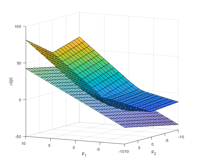
Figure 2: Plot of the function $\phi$ (top) described in Example 4.8, which appears to dominate the approximation $p\mapsto\phi(0)+\langle s,p\rangle$ (bottom) based on the computed compass difference $s$ of $\phi$ at $0$.

4.2.2 Optimal-value functions

A well-known result by Danskin [8, Theorem 1] describes directional derivatives for certain optimal-value functions, and has been extended to a variety of settings (e.g. [17, 3]). The following proposition and its proof are intended to show how any of these results may be combined with Theorem 3.4 or Corollary 3.10 to describe a subgradient in each case.

Proposition 4.9.

Consider a compact set $C\subset\mathbb{R}^{n}$, some open superset $Z$ of $C$, and a continuously differentiable function $f:\mathbb{R}^{2}\times Z\to\mathbb{R}$. Define an optimal-value function $\phi:\mathbb{R}^{2}\to\mathbb{R}$ for which

$$\phi:x\mapsto\min\{f(x,y):y\in C\}.$$

For some particular $\hat{x}\in\mathbb{R}^{2}$, define the following:

• a set $Y\coloneqq\{\hat{y}\in C:f(\hat{x},\hat{y})\leq f(\hat{x},y),\quad\forall y\in C\}$,

• for each $d\in\mathbb{R}^{2}$, a point $\psi(d)\coloneqq\min\{\langle d,\nabla_{x}f(\hat{x},y)\rangle:y\in Y\}$.

Then $\phi$ is locally Lipschitz continuous and directionally differentiable, and

$$\frac{1}{2}\begin{bmatrix}\psi(1,0)-\psi(-1,0)\\ \psi(0,1)-\psi(0,-1)\end{bmatrix}$$

is an element of $\partial\phi(\hat{x})$.

Proof 4.10.

The optimal-value function $\phi$ has already been established to be locally Lipschitz continuous [9, Theorem 2.1] and directionally differentiable [8], with directional derivatives given by ${\phi}^{\prime}(\hat{x};d)=\psi(d)$ for each $d\in\mathbb{R}^{2}$. The claimed result then follows immediately from Theorem 3.4.

Observe that, unlike several established sensitivity results for optimal-value functions [4, 5], the above result does not require second-order sufficient optimality conditions to hold, and does not require unique solutions of the optimization problems defining $\phi$. An analogous approach describes subgradients of the Tsoukalas-Mitsos convex relaxations [44] of composite functions of two variables; the Tsoukalas-Mitsos approach is based entirely on analogous optimal-value functions.

5 Conclusion

For a bivariate nonsmooth function under minimal assumptions, the compass difference introduced in this article is guaranteed to be a subgradient and may be computed using four calls to a directional-derivative evaluation oracle. This remains true for nonconvex functions, with the “subgradient” understood in this case to be an element of Clarke’s generalized gradient. Thus, for such functions, centered finite differences will necessarily converge to a subgradient as the perturbation width tends to zero. The presented examples show that this new relationship between directional derivatives and subgradients may be useful for functions of two variables, and may in some cases provide the only known way to evaluate a subgradient, but does not extend directly to functions of three or more variables. Such a nontrivial extension represents a possible avenue for future work.

References

- [1] C.Audet and W.Hare, Algorithmic construction of the subdifferential from directional derivatives, Set-Valued Var. Anal. 26 (2018), 431–447.
- [2] A.Bagirov, N.Karmitsa, and M. M.Mäkelä, Introduction to Nonsmooth Optimization: Theory, Practice, and Software, Springer, Cham, 2014.
- [3] D. P.Bertsekas, Nonlinear Programming, Athena Scientific, Nashua, 2nd edition, 1999.
- [4] J. F.Bonnans and A.Shapiro, Optimization problems with perturbations: A guided tour, SIAM Rev. 40 (1998), 228–264.
- [5] J. F.Bonnans and A.Shapiro, Perturbation Analysis of Optimization Problems, Springer Series in Operations Research, Springer, New York, 2000.
- [6] F. H.Clarke, Optimization and Nonsmooth Analysis, SIAM, Philadelphia, PA, 1990.
- [7] A. R.Conn, K.Scheinberg, and L. N.Vicente, Introduction to Derivative-Free Optimization, SIAM, Philadelphia, 2009.
- [8] J. M.Danskin, The theory of Max–Min, with applications, J. SIAM Appl. Math. 14 (1966), 641–664.
- [9] S.Dempe, B. S.Mordukhovich, and A. B.Zemkoho, Sensitivity analysis for two-level value functions with applications to bilevel programming, SIAM J. Optim. 22 (2012), 1309–1343.
- [10] F.Facchinei, A.Fischer, and M.Herrich, An LP-Newton method: nonsmooth equations, KKT systems, and nonisolated solutions, Math. Program., Ser. A 146 (2014), 1–36.
- [11] F.Facchinei and J. S.Pang, Finite-Dimensional Variational Inequalities and Complementarity Problems, Springer-Verlag New York, Inc., New York, NY, 2003.
- [12] A.Griewank, Automatic directional differentiation of nonsmooth composite functions, in Recent Developments in Optimization, French-German Conference on Optimization, Springer, Dijon, 1994.
- [13] A.Griewank and A.Walther, Evaluating Derivatives: Principles and Techniques of Algorithmic Differentiation, Other Titles in Applied Mathematics, SIAM, Philadelphia, PA, 2nd edition, 2008.
- [14] P.Hartman, Ordinary Differential Equations (2nd ed.), Classics in Applied Mathematics, SIAM, 2002.
- [15] J. B.Hiriart-Urruty and C.Lemaréchal, Convex Analysis and Minimization Algorithms I: Fundamentals, A Series of Comprehensive Studies in Mathematics, Springer-Verlag, Berlin, 1993.
- [16] J. B.Hiriart-Urruty and C.Lemaréchal, Convex Analysis and Minimization Algorithms II: Advanced Theory and Bundle Methods, A Series of Comprehensive Studies in Mathematics, Springer-Verlag, Berlin, 1993.
- [17] W.Hogan, Directional derivatives for extremal-value functions with applications to the completely convex case, Oper. Res. 21 (1973), 188–209.
- [18] C.Imbert, Support functions of the Clarke generalized Jacobian and of its plenary hull, Nonlinear Anal.-Theor. 49 (2002), 1111–1125.
- [19] K. A.Khan, Sensitivity analysis for nonsmooth dynamic systems, PhD thesis, Massachusetts Institute of Technology, 2015.
- [20] K. A.Khan, Relating lexicographic smoothness and directed subdifferentiability, Set-Valued Var. Anal. 25 (2017), 233–244.
- [21] K. A.Khan, Branch-locking AD techniques for nonsmooth composite functions and nonsmooth implicit funcitons, Optim. Method Softw. 33 (2018), 1127–1155.
- [22] K. A.Khan, Subtangent-based approaches for dynamic set propagation, in 2018 IEEE Conference on Decision and Control, IEEE, Miami Beach, 2018.
- [23] K. A.Khan and P. I.Barton, Generalized derivatives for solutions of parametric ordinary differential equations with non-differentiable right-hand sides, J. Optimiz. Theory App. 163 (2014), 355–386.
- [24] K. A.Khan and P. I.Barton, A vector forward mode of automatic differentiation for generalized derivative evaluation, Optim. Method Softw. 30 (2015), 1185–1212.
- [25] K. A.Khan and P. I.Barton, Generalized derivatives for hybrid systems, IEEE T. Automat. Contr. 62 (2017), 3193–3208.
- [26] K. C.Kiwiel, Methods of Descent for Nondifferentiable Optimization, Lecture Notes in Mathematics, Springer-Verlag, Berlin, 1985.
- [27] A. Y.Kruger, On Fréchet subdifferentials, J. Math. Sci. 116 (2003), 3325–3358.
- [28] C.Lemaréchal, J. J.Strodiot, and A.Bihain, On a bundle algorithm for nonsmooth optimization, in Nonlinear Programming 4, O. L.Mangasarian, R. R.Meyer, and S. M.Robinson (eds.), Academic Press, New York, NY, 1981.
- [29] L.Lukšan and J.Vlček, A bundle-Newton method for nonsmooth unconstrained minimization, Math. Program. 83 (1998), 373–391.
- [30] M. M.Mäkelä, Survey of bundle methods for nonsmooth optimization, Optim. Method. Softw. 17 (2002), 1–29.
- [31] B. S.Mordukhovich, Variational analysis and generalized differentiation I: Basic theory, Springer, Berlin, 2006.
- [32] Y.Nesterov, Lexicographic differentiation of nonsmooth functions, Math. Program. B 104 (2005), 669–700.
- [33] A.Neumaier, Interval Methods for Systems of Equations, Cambridge University Press, Cambridge, 1990.
- [34] J. S.Pang and D. E.Stewart, Solution dependence on initial conditions in differential variational inequalities, Math. Program. B 116 (2009), 429–460.
- [35] L.Qi, Convergence analysis of some algorithms for solving nonsmooth equations, Math. Oper. Res. 18 (1993), 227–244.
- [36] L.Qi and J.Sun, A nonsmooth version of Newton’s method, Math. Program. 58 (1993), 353–367.
- [37] R. T.Rockafellar and R. J. B.Wets, Variational Analysis, A Series of Comprehensive Studies in Mathematics, Springer, Berlin, 1998.
- [38] G.Rote, The convergence rate of the sandwich algorithm for approximating convex functions, Computing 48 (1992), 337–361.
- [39] S.Scholtes, Introduction to Piecewise Differentiable Equations, SpringerBriefs in Optimization, Springer, New York, NY, 2012.
- [40] N. Z.Shor, Minimization Methods for Non-Differentiable Functions, Springer Series in Computational Mathematics, Springer-Verlag, Berlin, 1985.
- [41] S. S.Skiena, Problems in geometric probing, Algorithmica 4 (1989), 599–605.
- [42] P. G.Stechlinski and P. I.Barton, Generalized derivatives of differential-algebraic equations, J. Optim. Theory App. 171 (2016), 1–26.
- [43] P. G.Stechlinski, K. A.Khan, and P. I.Barton, Generalized sensitivity analysis of nonlinear programs, SIAM J. Optim. 28 (2018), 272–301.
- [44] A.Tsoukalas and A.Mitsos, Multivariate McCormick relaxations, J. Glob. Optim. 59 (2014), 633–662.