The Formation Height of Millimeter-wavelength Emission in the Solar Chromosphere

Abstract

In the past few years, the ALMA radio telescope has become available for solar observations. ALMA diagnostics of the solar atmosphere are of high interest because of the theoretically expected linear relationship between the brightness temperature at mm wavelengths and the local gas temperature in the solar atmosphere. Key for the interpretation of solar ALMA observations is understanding where in the solar atmosphere the ALMA emission originates. Recent theoretical studies have suggested that ALMA bands at 1.2 (band 6) and 3 mm (band 3) form in the middle and upper chromosphere at significantly different heights. We study the formation of ALMA diagnostics using a 2.5D radiative MHD model that includes the effects of ion-neutral interactions (ambipolar diffusion) and non-equilibrium ionization of hydrogen and helium. Our results suggest that in active regions and network regions, observations at both wavelengths most often originate from similar heights in the upper chromosphere, contrary to previous results. Non-equilibrium ionization increases the opacity in the chromosphere so that ALMA mostly observe spicules and fibrils along the canopy fields. We combine these modeling results with observations from IRIS, SDO and ALMA to suggest a new interpretation for the recently reported “dark chromospheric holes”, regions of very low temperatures in the chromosphere.

1 Introduction

To better understand the origin of heating and dynamics in the solar chromosphere, it is important to reliably diagnose thermodynamic and magnetic field conditions in this important region in the solar atmosphere (for a review Carlsson et al., 2019). Typically, observational constraints in the chromosphere are derived from spectral lines that are optically thick and formed under conditions of non Local Thermodynamic Equilibrium (non-LTE), such as Ca II 8542Å  (Cauzzi et al., 2009), H$\alpha$ (Rutten, 2008; Leenaarts et al., 2012) or Mg II h 2803Å and k 2796Å  (Schmit et al., 2015). The interpretation of these diagnostics can be complicated, as the line formation depends on complex radiative transfer effects such as partial frequency redistribution (PRD) and 3D scattering (e.g., Leenaarts et al., 2012), as well as on time dependent ionization (at least for Ca II and H$\alpha$, Wedemeyer-Böhm & Carlsson, 2011; Leenaarts et al., 2007, 2013). ALMA observations potentially offer an attractive alternative (or rather complement, given the paucity of ALMA solar observations), as they do not suffer from some of these effects.

The advent of solar observations at ALMA has led to several recent publications that summarize the potential of radio observations to provide direct measurements of the plasma temperature for a wide range of heights in the chromosphere (see Wedemeyer et al., 2016, review). Such measurements would provide novel diagnostics of chromospheric physical processes and direct constraints on state-of-the-art numerical models of the chromosphere. However, for a proper interpretation of ALMA observations, it is important to understand where the diagnostics originate, especially given the highly dynamic state of the chromosphere (which is strongly impacted by, e.g., magneto-acoustic shocks Carlsson et al., 1997).

Current best estimates of the formation height of ALMA diagnostics and the relationship between observed brightness temperature and local gas temperature (Wedemeyer et al., 2016) are based on 3D radiative MHD (rMHD) models of relatively quiet regions (Carlsson et al., 2016) in which hydrogen is treated in non-equilibrium ionization (NEI) (Loukitcheva et al., 2015a). These models suggest that there is a good relationship between brightness temperature and local temperature, and that the various ALMA bands are formed at different heights in the low to upper chromosphere. Such models have also been used to analyze the benefits of combining ALMA and NUV observations from the Interface Region Imaging Spectrograph (IRIS, see De Pontieu et al., 2014) in order to derive semiempirical models from the inversion of the observed intensities (da Silva Santos et al., 2018). Similarly, Loukitcheva et al. (2015a) used a 3D rMHD simulation to assess the potential of using ALMA observations to study chromospheric magnetic fields. However, the numerical simulations utilized in those publications were only representative of quiet Sun conditions. In addition, these models have not simultaneously included the effects of ion-neutral interactions in the partially ionized chromosphere, time-dependent ionization and/or missing physical processes such as the formation of type II spicules.

For the first time, we analyze the formation of ALMA intensities from a very high spatial resolution simulation that is representative of the dynamics, magnetic field configuration and fine structuring of plage and strong network regions on the Sun. The simulations utilized in the present study include time-dependent ionization of both hydrogen and helium, interactions between neutral and ionized particles, and the full stratification of the atmosphere from the upper convection zone to the corona. To better understand the effects of time dependent ionization, we use two simulations, one with and one without NEI. We describe briefly the numerical simulations (Section 2) and ALMA synthetic calculations (Section 3). In Section 4 we describe our results and show that the formation height and the integration along the line-of-sight (LOS) of the brightness temperature are highly dependent on the electron density which is drastically increased in the upper chromosphere as a result of time dependent ionization and the increased mass loading resulting from spicular flows. These results dramatically change the interpretation of ALMA observations, indicating that in many regions these are dominated by fibrils and spicules along the magnetic canopy, bringing them more in line with expectations from theoretical approaches inspired by H$\alpha$ observations (Rutten, 2017). We also discuss how our results offer a new interpretation for the recently discovered “chromospheric holes” (Loukitcheva et al., 2019) and finish with conclusions (Section 5).

2 Numerical simulations

We use the two different 2.5D rMHD numerical simulations analyzed in Martinez-Sykora et al. (2019). These simulations have been calculated with the 3D rMHD Bifrost code (Gudiksen et al., 2011) including scattering (Skartlien, 2000; Hayek et al., 2010; Carlsson & Leenaarts, 2012), thermal conduction along the magnetic field, and ion-neutral effects, i.e., ambipolar diffusion and Hall term (Martínez-Sykora et al., 2012, 2017; Nóbrega-Siverio et al., 2019). The simulations differ in their treatment of the ionization balance: the gol_lte simulation is in LTE, while the gol_nei simulation computes the ionization balance in non-equilibrium for hydrogen and helium (Leenaarts et al., 2007; Golding et al., 2014).

In both simulations, the numerical domain covers a region that is $90$ Mm wide and that covers a height range from 3 Mm below to 40 Mm above the photosphere. The horizontal resolution is uniform with a $14$ km grid spacing, while the vertical resolution is non-uniform with the largest resolution in the photosphere, chromosphere and transition region ($\sim 12$ km grid spacing). The magnetic field configuration includes two plage regions of opposite polarity with an unsigned mean magnetic field of $\sim 190$ G, and loops connecting both polarities (Figure 1A).

The boundary conditions are periodic in the horizontal direction and open in the vertical direction, allowing waves and plasma to go through. In addition, the bottom boundary has a constant entropy in regions of inflow to maintain the solar convective motions with $\sim 5780$ K effective temperature at the photosphere. Further details on the setup and analysis of these two simulations can be found in Martinez-Sykora et al. (2019) and in Martínez-Sykora et al. (2017) for the gol_lte simulation.

3 Synthesis of ALMA observations

To compute synthetic observations from our simulations in the ALMA observations at 1.2 (ALMA band 6) and 3 mm (ALMA band 3), we used the LTE module in the Stockholm inversion code (STiC) code (de la Cruz Rodríguez et al., 2016, 2019). STiC utilizes the electron densities and gas pressure stratifications from the simulations to compute the partial densities of all species that are involved in the calculations. Continuum opacities are calculated using routines ported from the ATLAS code (Kurucz, 1970), which include the main opacity source at mm wavelengths (free-free hydrogen absorption, see Wedemeyer et al. 2016). The emergent intensity is calculated using a formal solver of the unpolarized radiative transfer equation based on cubic-Bezier splines (Auer, 2003; de la Cruz Rodríguez & Piskunov, 2013).

4 Results

4.1 Formation height of ALMA observations

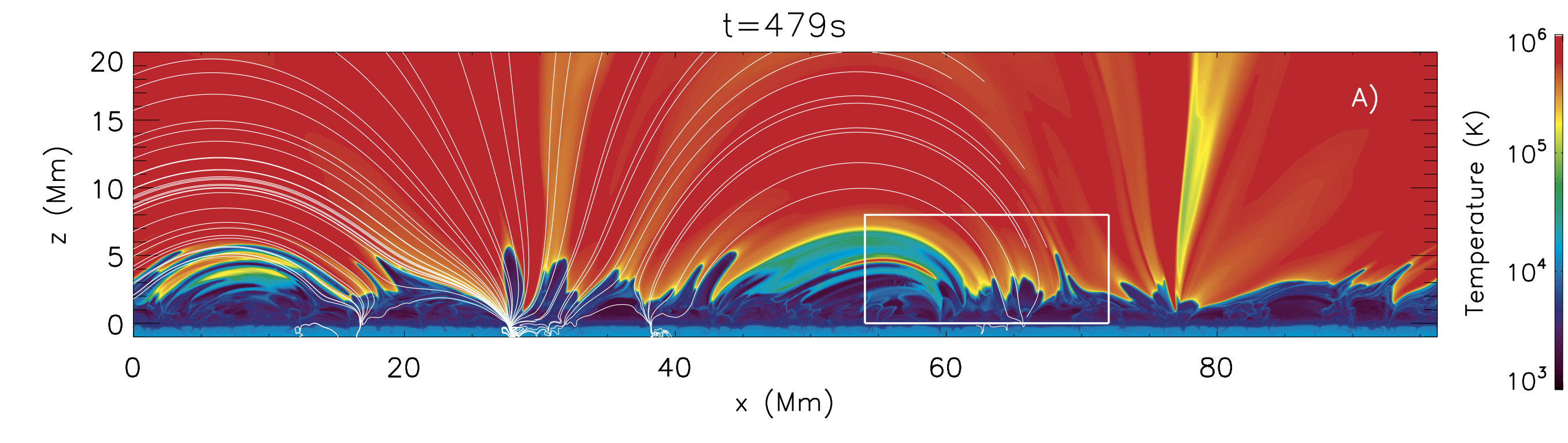
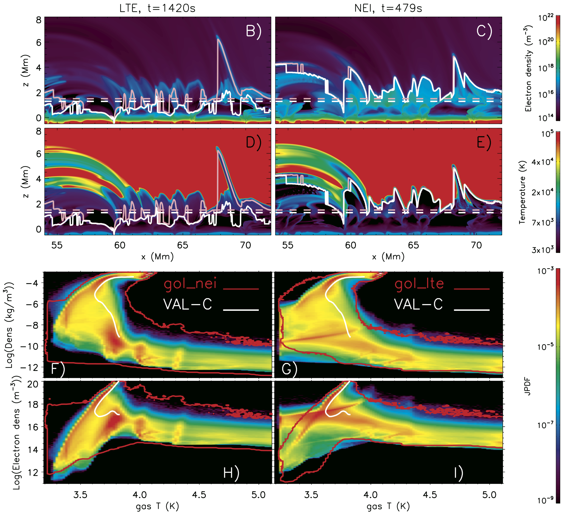
Figure 1: The formation height of ALMA passbands depends on the thermodynamic state of the chromosphere which is impacted significantly by ion-neutral interactions and NEI. Panel A shows the temperature in the gol_nei  simulation. For clarity, magnetic field lines are shown only in the left half of the numerical domain. Panels B-E zoom in on the white box in panel A, with maps of electron density (B, C) and temperature (D, E) for the gol_lte (left), and gol_nei (right) simulations. Formation height ($\tau=1$) of observations at 3 and 1.2mm are shown with pink and white lines, respectively. The dashed lines correspond to $\tau=1$ for the VAL-C model for the corresponding mm observations. Panels F-I show joint probability density functions (JPDF) of temperature and density (F, G) and of temperature and electron number density (H, I), each computed from a time series of 12 minutes of solar time. For comparison between both simulations, we include the red contours which correspond to the temperature and density regime (of the whole simulation) at JPDF$=5\times 10^{-5}$ for the other simulation (see labels). The white line corresponds to the VAL-C model.

In order to address the typical formation height of ALMA observations, we computed the optical depth ($\tau$) at 1.2 and 3mm wavelengths (ALMA bands 6 and 3, respectively). Figure 1 shows maps of electron number density (panels B and C) and temperature (panels D and E) for the gol_lte (left), and gol_nei (right) simulations. Overplotted are white and pink solid lines which show the heights for which $\tau=1$ for observations at 3 and 1.2mm, respectively. Under LTE conditions, the $\tau=1$ heights at 3mm are well separated from $\tau=1$ heights at 1.2mm. The latter typically occur within $0.5-2$ Mm above the photosphere, i.e., lower-mid chromosphere and often form within the cold expanding bubbles produced in the wake of magneto-acoustic shocks. Averaged over 12 minutes in the numerical simulation, the average formation height at wavelengths of 1.2mm is 0.9 Mm (with a standard deviation of 0.7 Mm). Observations at 3mm are formed at significantly greater heights and often forms along type II spicules. As a result, the average formation height at 3mm is 1.8 Mm (standard deviation of 1 Mm). The mean difference of the formation heights at these wavelengths is 0.92 ($\pm 0.85$ Mm).

Under NEI conditions, the electron density (panels C and I) is much higher within the chromosphere than in LTE (panels B and H). On average the 1.2mm emission is formed at a height of $2.67\pm 1.08$ Mm, while the 3mm emission is formed at a mean height of $2.78\pm 1.09$ Mm. The difference in average formation heights of these wavelengths is thus $0.11\pm 0.3$ Mm.This can be explained as follows. In NEI, the recombination timescales are much longer than the MHD timescales. This means that during the passage of shocks (a key constituent of chromospheric dynamics), the cooling from expanding bubbles in the wake of shocks leads to a decrease of the plasma temperature instead of the recombination that would occur under LTE conditions. Consequently, the formation height for both wavelengths is moved to significantly greater heights in the upper-chromosphere, near the transition region. In fact, most of the time and almost everywhere these two wavelengths observe very similar regions: low-lying loops, fibrils or/and spicules. The impact of NEI on the formation height is thus significant and fundamentally alters the interpretation of the ALMA observations.

For comparison we add, for both ALMA wavelengths, the height at which the optical depth is unity for a VAL-C (Vernazza et al., 1981) atmosphere (dashed horizontal lines in Figure 1B-E). It is clear that the large variability of the formation height of these two wavelengths in a rMHD model is not captured by the VAL-C model.

It is important to note that the chromosphere is highly structured, with large temperature and density (or electron density) variations. This is clearly shown with the Joint Probability Distributions Functions (JPDF) of temperature and density, and temperature and electron number density shown in Figure 1F-I. Note that the JDPF’s axes are in logarithmic scale. We refer the reader to Martinez-Sykora et al. (2019) for details on the differences of these thermal properties between the gol_lte and gol_nei simulations.

The temperature variations within the chromosphere are greatest in the gol_nei simulation because any heating or cooling due to various entropy sources (e.g., ambipolar heating or work) change the temperature instead of recombining or ionizing the plasma. The VAL-C model cannot reveal these variations (white line in Figure 1F-I). The three preferred temperatures at $\log(T/K)=3.8$, 4 and 4.3 in the LTE case (panels F-G) correspond to the ionization temperatures of hydrogen and helium (Leenaarts et al., 2007; Golding et al., 2016). In NEI, these three bands smear out (panels H-I). In addition, in NEI, plasma seems to follow an adiabatic relation ($T=[10^{3.2},10^{4}]$ K, $\rho=[10^{-10},10^{-8}]$ kg m^-3, and $n_{e}=[10^{17},10^{18}]$ m^-3). This is due to fact that the cooling from the expansion in the wake of acoustic shocks (in the low chromosphere, along spicules, and along low-lying loops) will not lead to recombination (because of the long timescales involved in NEI). As mentioned above, this leads to a much larger electron density and opacities in NEI than in LTE (up to 4 orders of magnitude). So, the NEI changes completely the electron density distribution within the chromosphere and therefor the formation height at 3 and 1.2mm as shown in panels B-E.

4.2 Relationship between ALMA brightness temperature and plasma temperature

Given that NEI changes the formation height of ALMA observations, we now consider the diagnostic capability of ALMA in our models. In particular, we want to address whether the observed brightness temperature ($Tb$) is correlated with the local gas temperature at $\tau=1$. The left column of Figure 2 shows the synthetic $Tb$ at 3 and 1.2mm (red) and the gas temperature at their corresponding $\tau=1$ (black). Observations at 3mm show greater variability in space than at 1.2mm, both in LTE and NEI. One can see that there is some correlation between the two temperatures. However, in several locations the discrepancy between the two temperatures, in both LTE and NEI, can reach up to a few $10^{3}$ K.

To further illustrate this, we calculated the JPDF of the gas temperature at $\tau=1$ and $Tb$ (right column in Figure 2). The JPDFs show some correlation between the two temperatures, which visually appears to be somewhat better for the NEI case. However, the standard deviation of the difference between $Tb$ and the gas temperature ($\sigma$, bottom-right labels in the right column of Figure 2) is larger in NEI than in LTE. Observations at 1.2mm provide a better match with the gas temperature than at 3mm. Still, the correlation is far from perfect and limits the degree to which ALMA observations can constrain numerical models. The discrepancy between the two temperatures is caused by the LOS integration as detailed below.

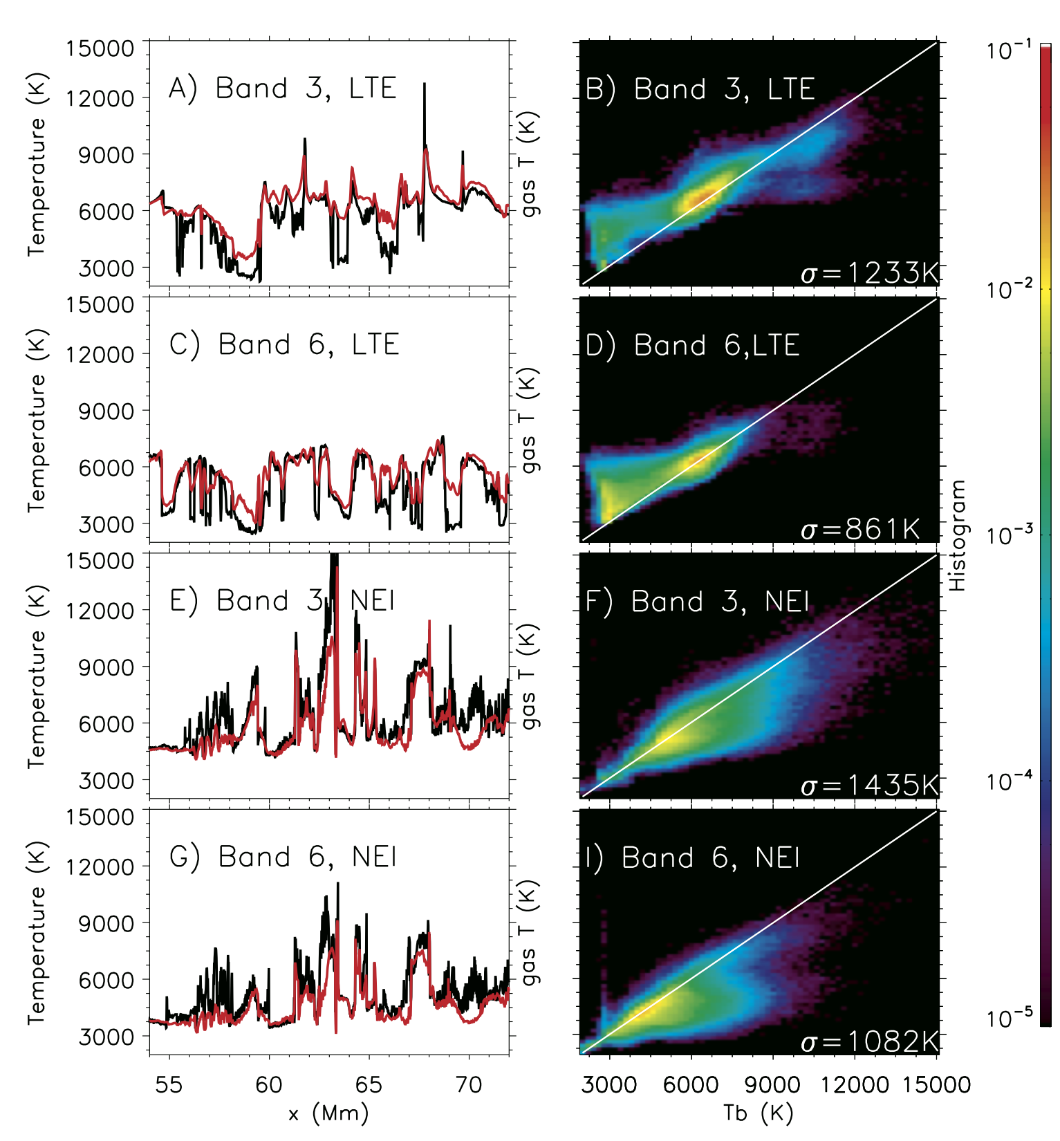
Figure 2: Synthetic ALMA observations (red) can differ from the gas temperature at $\tau=1$ (black) by several $10^{3}$ K. Synthetic ALMA observations at 3mm (odd rows) and at 1.2mm (even rows) are shown for for gol_lte (top two rows) and gol_nei (bottom two rows). Left column shows the JPDF between the synthetic ALMA observations (x-axis) and gas temperature at $\tau=1$ (y-axis).

To investigate the LOS effects, we calculated the contribution function and the source function for both wavelengths (Figure 3). In LTE, the contributions to the total intensity are formed over a wide range of heights, often with parcels at very different heights equally contributing. As we know, the ionization in LTE is highly underestimated because, in NEI, the recombination time-scales are larger than the timescales related to magneto-acoustic evolution or associated with other entropy sources (e.g., ambipolar heating, Martinez-Sykora et al., 2019). The fact that in LTE very different packets of plasma along the LOS contribute to the brightness temperature leads to the lower degree of correlation between these two temperatures (as compared to the NEI case).

In contrast, the contribution function for the NEI case is more confined to a narrow region along the LOS: $\tau=1$ occurs at much greater heights, which significantly reduces the number of plasma elements above that height that can contribute. Despite the general visual impression of a somewhat better overall correlation between brightness and plasma temperature for the NEI case, we nevertheless find a larger standard deviation $\sigma$ (i.e., worse correlation). This is because in the gol_nei simulation extremely sharp and large variations arise in the source functions in comparison to the gol_lte simulation (right column of Figure 3). These are caused by the stronger temperature gradients within the chromosphere in the gol_nei simulation (see Martinez-Sykora et al., 2019, for details). These in turn are caused by the fact that any heating or cooling changes the gas temperature instead of ionizing or recombining the plasma. This results in large temperature variations rather than preferentially keeping the plasma around the ionization temperatures (Figure 1F-I).

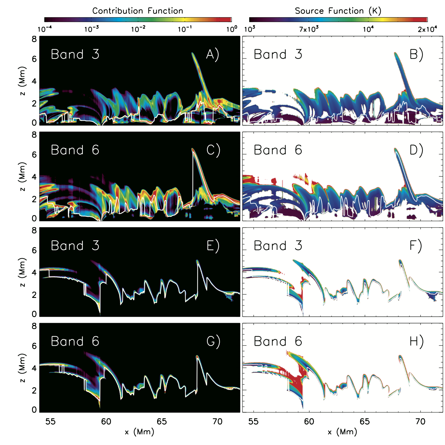
Figure 3: The impact from LOS integration on the synthetic observations at 1.2 (even rows) and 3mm (odd rows) for the gol_lte (two top rows) and gol_nei simulations (two bottom rows). Left column shows the contribution function normalized to the highest values along the LOS ($CF$). Right column is the source function where we masked regions with $CF<10^{-4}$. The formation height ($\tau=1$) of the corresponding observations are shown with white lines.

In summary, since the formation height of the ALMA observations occurs at greater heights in NEI than in LTE, the LOS superposition is much smaller for the former. However, this is counteracted by the fact that the gol_nei simulation has sharper transitions in temperature. As a result, even if the LOS is integrated over a narrower region, the LOS effects become more important.

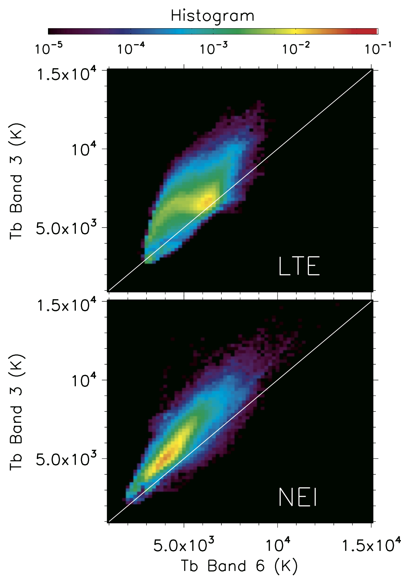
Figure 4: The JPDF between the brightness temperatures at 3 and 1.2mm show a good correlation for the NEI case (bottom), in contrast to the LTE case (top).

Given the close proximity of the typical formation heights, the question arises whether these different wavelengths have significantly different diagnostic capability for the NEI case. Panels F and H in Figure 3 show that the source function is very similar for both wavelengths. It is then not surprising that the JPDF between at 3 and 1.2mm (Figure 4) shows a strong correlation for the gol_nei simulation (contrary to the LTE case). The lack of correlation in the LTE case is expected (top panel), as these wavelengths are formed in very different regions. However, in NEI, the correlation between 3 and 1.2mm is actually better than the correlation between $Tb$ and gas temperatures shown in Figure 2F and I. We find a significant difference in average temperatures between 3 and 1.2mm, as the former is formed at slightly greater heights, essentially in the same structures. The mean brightness temperature difference between the two wavelengths is $1280$ K. This results from strong temperature gradients within the structures (e.g, perpendicular to the magnetic field direction in low-lying loops or inclined spicules). If these findings are borne out by comparisons between 3 and 1.2mm observations (hampered by the lack of simultaneity between wavelengths), our findings suggest that observations at 1.2mm might be preferred, given the higher spatial resolution that can be obtained using ALMA and the slightly better correlation with gas temperature at $\tau=1$ (Figure 2). If 3 and 1.2mm observations were close to simultaneously possible, they might help identify locations of sharp temperature gradients.

4.3 Alternative observational interpretations

Our results can also be used to provide a new interpretation of recent ALMA observations by Loukitcheva et al. (2019) who reported regions of low brightness temperature and named these “chromospheric holes”, suggesting a possible link to previous observations of low-lying cool gas deduced from molecular CO lines.

Here we present a different possible scenario using our simulations and combining with observations using SDO/AIA (Lemen et al., 2012), IRIS and ALMA band3 observations. Both ALMA and IRIS observed the same region through a coordinated ALMA/IRIS campaign (Figure 5). The IRIS observing program was centered at heliocentric coordinates of 170″, -210″, with a medium (i.e., 60″ FOV along the slit), coarse (i.e., 2″ steps), 16-step raster with an exposure time per slit position of 2s and a raster cadence of 32s. The ALMA interferometric data were acquired on 2017/04/27 in Band 3 (at 3mm, i.e., 100 GHz) in configuration C40-3 (see Loukitcheva et al., 2019, for further details). ALMA obtained 10.5 minute scans separated by 2min calibration scans, with 2s integration time, for a total of 37min within 16:00-16:45 UT (45 minutes). The ALMA data we show here is averaged over that time interval. ALMA solar observations are detailed in Shimojo et al. (2017); White et al. (2017).

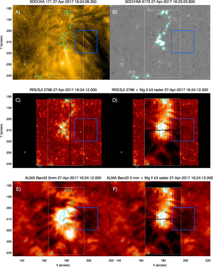
Figure 5: Analysis of IRIS spectroheliograms, SDO/AIA-HMI and ALMA observations suggests that low-lying fibrils occur in the same region as where Loukitcheva et al. (2019) (in their Figure 1) reported the presence of a “chromospheric hole” region of low brightness temperature using ALMA observations. Panel A shows an SDO/AIA 171 Å image; panel B shows an SDO/HMI magnetogram (scaled to $\pm 200$ G); panel C shows an IRIS 2796 slit-jaw image, while panel D shows a spectroheliogram (averaged over the same 45 minute time period as the ALMA observations) at the core of the Mg II k line (superimposed on top of the IRIS 2796 slit-jaw image); panel E shows the time-averaged relative brightness temperature in ALMA band3, while panel F includes the time-integrated Mg II 2796 Å k3 spectroheliogram. Green contours correspond to $100$ G in panel B and the blue box outlines the region of low ALMA brightness temperature from Loukitcheva et al. (2019) (see their Figure 1).

While it is difficult to determine the morphology of the chromospheric hole region from the 2796 SJI images, the IRIS spectroheliogram at the core of the Mg II 2796 Å k3 line shows clear evidence of long fibrils, commonly seen outlining low-lying canopy fields originating from stronger field regions. The SDO/HMI magnetograms (panel B and green contours) confirm that these fibrils do indeed connect to a strong magnetic field region with significant magnetic field strength ($>100~{}$G), i.e., a decayed plage or enhanced network region. In addition, timeseries of SDO/AIA 171Å images similarly reveal a mix of dark and bright features compatible with low-lying fibrils in the “chromospheric hole” region (blue box). Detailed inspection of ALMA band3, the integrated-in-time IRIS Mg II 2796 Å k3 spectroheliogram, and SDO/AIA 171 observations shows fibril-like features with similar morphology in all three observations. Further details of the ALMA observational analysis can be found in Loukitcheva et al. (2019).

Given this observational context, our simulations indicate that such areas of “low-lying loops outlining the canopy that originates from strong field regions” should have low brightness temperatures. For example, the region between 55 and 60 Mm (in x) in Figure 1 shows that the low-lying loops are sites of very high electron density (i.e., high opacity in ALMA) with low temperatures, as low as 3,500-4,500K (Figure 2). This is very similar to what is reported for “chromospheric holes” by Loukitcheva et al. (2019). In our simulations, the ALMA observations of low temperatures arise from low-temperature sub-threads in low-lying loops, a natural consequence of the chromospheric dynamics when taking into account mass loading from spicules, heating from shocks and ambipolar diffusion, and NEI effects. For details on these structures, we refer the reader to Martinez-Sykora et al. (2019).

We also note that the high ALMA $Tb$ near the footpoints of the fibrils (Figure 1A in Loukitcheva et al., 2019) matches the shape of the bright region in the Mg II 2796 Å k3 spectroheliogram (panel D). Our simulations suggest that these high temperatures may be caused by the spicules and associated heating at the footpoints of the low-lying fibrils.

5 Conclusions and discussion

We have used two different state-of-the-art 2.5D rMHD simulations (one assuming LTE ionization, one assuming NEI), both including ion-neutral interaction effects, to investigate the formation height and diagnostic capability of the ALMA bands 3 (3mm) and 6 (1.2mm) observations. Our results show that NEI, and the strong mass loading in the upper chromosphere (arising from heating caused by ambipolar diffusion, as well as spicules and shocks), both have a significant impact on the interpretation of ALMA observations.

In our NEI model, the formation height of ALMA at both wavelengths occurs at greater heights than in LTE models. In addition, both wavelengths observe roughly the same features and region.

Previous studies (e.g., Loukitcheva et al., 2015b) focused on understanding ALMA observations using numerical models that did not include spicular mass loading or ambipolar diffusion/heating (Carlsson et al., 2016). They also typically did not compare LTE versus NEI with the exception of Leenaarts & Wedemeyer-Böhm (2006). However, our results seem to be contrary to Leenaarts & Wedemeyer-Böhm (2006): it is unclear in their results if the ALMA formation height in NEI is at greater heights than in LTE. This is most likely because their model is much shallower (only up to the lower chromosphere) and did not include the greater densities in the upper chromosphere seen in our 2.5D rMHD models that include ambipolar diffusion. As a result, their model did not show the large electron density and opacities at greater heights that appears in NEI, and it did not couple the NEI effects to the hydrodynamics.

Our 2.5D rMHD model including NEI differs from previous work (e.g., Wedemeyer-Böhm et al., 2007; Loukitcheva et al., 2015b) in several ways: 1) our model includes more physical processes, i.e., non-equilibrium hydrogen and helium ionization, as well as ambipolar diffusion; 2) our magnetic field configuration mimics a plage or strong network region, while previous models typically mimicked very quiet Sun and/or smaller numerical domains; 3) our model has higher densities and opacities in the upper atmosphere due to the presence of low-lying loops and spicules, 4) our model has higher spatial resolution, e.g, more than four times better resolution than the simulation used in Loukitcheva et al. (2015b).

Our models show that due to the high opacities in the upper chromosphere from the presence of type II spicules, low lying loops and large-scale magnetic field configuration, and taking into account the NEI effects, the formation height of both wavelengths is located in the upper chromosphere. Due to the hydrogen and helium NEI and the ambipolar diffusion, the plasma has very large temperature variations along the LOS.

Our results are well aligned with predictions from Rutten (2017) who theorizes that ALMA mm observations will show opacities that are similar or larger than H$\alpha$. Consequently, he predicts that ALMA will mostly observe fibrils along the canopy, while anything below will be masked by these fibrils. Molnar et al. (2019) found that ALMA band 3 correlates nicely with H$\alpha$ core width. Our gol_nei simulation which includes NEI, also shows large ALMA opacities in the upper chromosphere which mask anything below. Consequently, contributions at 1.2 and 3mm are confined to the upper chromosphere, i.e., low-lying loops (canopy fibrils), and spicules, instead of the acoustic shocks in the lower atmosphere (Wedemeyer et al., 2016).

Although the contribution functions for both wavelengths are confined to a very narrow region in the gol_nei simulation, our NEI results show that care must be taken when interpreting ALMA brightness temperatures as a local gas temperature. Not only is there a large spread in the correlation between these quantities, the plasma also shows very large temperature gradients along the LOS since any cooling or heating will change the plasma temperature instead of being amortized by ionization or recombination. In addition, spicules and low-lying loops may contain thin threads of very different temperatures (Martinez-Sykora et al., 2019). Our results suggest that emission at 1.2mm and 3mm is formed at similar (but not identical) heights in the solar atmosphere. Consequently, the comparison between emission at these two wavelengths can provide information about temperature gradients (e.g., within the same feature). Our NEI model of active region and enhanced network shows a mean brightness temperature difference of 1280 K between the two wavelengths. This is similar to the difference in mean brightness temperature between the two ALMA bands of 1400 K in the averaged over the whole Sun White et al. (2017). Note that these observations include both AR and QS, although the latter dominates in terms of areal coverage.

One main reason for the different results in the current work (compared to previous work) is the fact that our simulations show large opacities in the upper chromosphere. Analysis has shown that this is caused by several factors: the inclusion of ambipolar diffusion, as well as the inclusion of both large-scale and small-scale magnetic field structures. In previous work, due to the small numerical domain, typically, the magnetic field expands drastically with height, diluting shocks and other drivers of mass flows, so that it has been very difficult to reach high densities in the upper chromosphere (Martínez-Sykora et al., 2013; Carlsson et al., 2016).

As with any numerical model, care should be taken when applying it to the real Sun. We note that our model is limited to two dimensions, and it is crucial to expand this model into 3D. Nevertheless, we expect that in plage and strong network regions the field will not suffer as much expansion with height as quiet Sun models in 3D. One should also keep in mind that models tend to simplify the magnetic structure and may limit the LOS superposition compared to what happens on the Sun.

Nevertheless and in conclusion, our results indicate that state-of-the-art inversions and/or synthetic observations from rMHD models need to take into account NEI effects for a proper interpretation of ALMA observations.

References

- Auer (2003) Auer, L. 2003, Astronomical Society of the Pacific Conference Series, Vol. 288, Formal Solution: EXPLICIT Answers, ed. I. Hubeny, D. Mihalas, & K. Werner, 3
- Carlsson et al. (2019) Carlsson, M., De Pontieu, B., & Hansteen, V. H. 2019, ARA&A, 57, 189, doi: 10.1146/annurev-astro-081817-052044
- Carlsson et al. (2016) Carlsson, M., Hansteen, V. H., Gudiksen, B. V., Leenaarts, J., & De Pontieu, B. 2016, A&A, 585, A4, doi: 10.1051/0004-6361/201527226
- Carlsson et al. (1997) Carlsson, M., Judge, P. G., & Wilhelm, K. 1997, ApJ, 486, L63, doi: 10.1086/310836
- Carlsson & Leenaarts (2012) Carlsson, M., & Leenaarts, J. 2012, A&A, 539, A39, doi: 10.1051/0004-6361/201118366
- Cauzzi et al. (2009) Cauzzi, G., Reardon, K., Rutten, R. J., Tritschler, A., & Uitenbroek, H. 2009, A&A, 503, 577, doi: 10.1051/0004-6361/200811595
- da Silva Santos et al. (2018) da Silva Santos, J. M., de la Cruz Rodríguez, J., & Leenaarts, J. 2018, A&A, 620, A124, doi: 10.1051/0004-6361/201833664
- de la Cruz Rodríguez et al. (2016) de la Cruz Rodríguez, J., Leenaarts, J., & Asensio Ramos, A. 2016, ApJ, 830, L30, doi: 10.3847/2041-8205/830/2/L30
- de la Cruz Rodríguez et al. (2019) de la Cruz Rodríguez, J., Leenaarts, J., Danilovic, S., & Uitenbroek, H. 2019, A&A, 623, A74, doi: 10.1051/0004-6361/201834464
- de la Cruz Rodríguez & Piskunov (2013) de la Cruz Rodríguez, J., & Piskunov, N. 2013, ApJ, 764, 33, doi: 10.1088/0004-637X/764/1/33
- De Pontieu et al. (2014) De Pontieu, B., Title, A. M., Lemen, J. R., et al. 2014, Sol. Phys., 289, 2733, doi: 10.1007/s11207-014-0485-y
- Golding et al. (2014) Golding, T. P., Carlsson, M., & Leenaarts, J. 2014, ApJ, 784, 30, doi: 10.1088/0004-637X/784/1/30
- Golding et al. (2016) Golding, T. P., Leenaarts, J., & Carlsson, M. 2016, ApJ, 817, 125, doi: 10.3847/0004-637X/817/2/125
- Gudiksen et al. (2011) Gudiksen, B. V., Carlsson, M., Hansteen, V. H., et al. 2011, A&A, 531, A154+, doi: 10.1051/0004-6361/201116520
- Hayek et al. (2010) Hayek, W., Asplund, M., Carlsson, M., et al. 2010, A&A, 517, A49+, doi: 10.1051/0004-6361/201014210
- Kurucz (1970) Kurucz, R. L. 1970, SAO Special Report, 309
- Leenaarts et al. (2007) Leenaarts, J., Carlsson, M., Hansteen, V., & Rutten, R. J. 2007, A&A, 473, 625, doi: 10.1051/0004-6361:20078161
- Leenaarts et al. (2012) Leenaarts, J., Carlsson, M., & Rouppe van der Voort, L. 2012, ApJ, 749, 136, doi: 10.1088/0004-637X/749/2/136
- Leenaarts et al. (2013) Leenaarts, J., Pereira, T. M. D., Carlsson, M., Uitenbroek, H., & De Pontieu, B. 2013, ApJ, 772, 89, doi: 10.1088/0004-637X/772/2/89
- Leenaarts & Wedemeyer-Böhm (2006) Leenaarts, J., & Wedemeyer-Böhm, S. 2006, in Astronomical Society of the Pacific Conference Series, Vol. 354, Solar MHD Theory and Observations: A High Spatial Resolution Perspective, ed. J. Leibacher, R. F. Stein, & H. Uitenbroek, 306
- Lemen et al. (2012) Lemen, J. R., Title, A. M., Akin, D. J., et al. 2012, Sol. Phys., 275, 17, doi: 10.1007/s11207-011-9776-8
- Loukitcheva et al. (2015a) Loukitcheva, M., Solanki, S. K., Carlsson, M., & White, S. M. 2015a, A&A, 575, A15, doi: 10.1051/0004-6361/201425238
- Loukitcheva et al. (2015b) Loukitcheva, M., Solanki, S. K., White, S. M., & Carlsson, M. 2015b, in Astronomical Society of the Pacific Conference Series, Vol. 499, Revolution in Astronomy with ALMA: The Third Year, ed. D. Iono, K. Tatematsu, A. Wootten, & L. Testi, 349. https://arxiv.org/abs/1508.05686
- Loukitcheva et al. (2019) Loukitcheva, M. A., White, S. M., & Solanki, S. K. 2019, ApJ, 877, L26, doi: 10.3847/2041-8213/ab2191
- Martínez-Sykora et al. (2017) Martínez-Sykora, J., De Pontieu, B., Carlsson, M., et al. 2017, ApJ, 847, 36, doi: 10.3847/1538-4357/aa8866
- Martínez-Sykora et al. (2012) Martínez-Sykora, J., De Pontieu, B., & Hansteen, V. 2012, ApJ, 753, 161, doi: 10.1088/0004-637X/753/2/161
- Martinez-Sykora et al. (2019) Martinez-Sykora, J., Leenaarts, J., De Pontieu, B., et al. 2019, arXiv e-prints, arXiv:1912.06682. https://arxiv.org/abs/1912.06682
- Martínez-Sykora et al. (2013) Martínez-Sykora, J., De Pontieu, B., Leenaarts, J., et al. 2013, ApJ, 771, 66, doi: 10.1088/0004-637X/771/1/66
- Molnar et al. (2019) Molnar, M. E., Reardon, K. P., Chai, Y., et al. 2019, ApJ, 881, 99, doi: 10.3847/1538-4357/ab2ba3
- Nóbrega-Siverio et al. (2019) Nóbrega-Siverio, D., Martínez-Sykora, J., Moreno-Insertis, F., & Carlsson, M. 2019, in preparation
- Rutten (2008) Rutten, R. J. 2008, Astronomical Society of the Pacific Conference Series, Vol. 397, H as a Chromospheric Diagnostic, ed. S. A. Matthews, J. M. Davis, & L. K. Harra, 54
- Rutten (2017) —. 2017, A&A, 598, A89, doi: 10.1051/0004-6361/201629238
- Schmit et al. (2015) Schmit, D., Bryans, P., De Pontieu, B., et al. 2015, ApJ, 811, 127, doi: 10.1088/0004-637X/811/2/127
- Shimojo et al. (2017) Shimojo, M., Bastian, T. S., Hales, A. S., et al. 2017, Sol. Phys., 292, 87, doi: 10.1007/s11207-017-1095-2
- Skartlien (2000) Skartlien, R. 2000, ApJ, 536, 465, doi: 10.1086/308934
- Vernazza et al. (1981) Vernazza, J. E., Avrett, E. H., & Loeser, R. 1981, ApJS, 45, 635, doi: 10.1086/190731
- Wedemeyer et al. (2016) Wedemeyer, S., Bastian, T., Brajša, R., et al. 2016, Space Sci. Rev., 200, 1, doi: 10.1007/s11214-015-0229-9
- Wedemeyer-Böhm & Carlsson (2011) Wedemeyer-Böhm, S., & Carlsson, M. 2011, A&A, 528, A1, doi: 10.1051/0004-6361/201016186
- Wedemeyer-Böhm et al. (2007) Wedemeyer-Böhm, S., Ludwig, H. G., Steffen, M., Leenaarts, J., & Freytag, B. 2007, A&A, 471, 977, doi: 10.1051/0004-6361:20077588
- White et al. (2017) White, S. M., Iwai, K., Phillips, N. M., et al. 2017, Sol. Phys., 292, 88, doi: 10.1007/s11207-017-1123-2