Binary Classification from Positive Data with Skewed Confidence

Abstract

Positive-confidence (Pconf) classification [Ishida et al., 2018] is a promising weakly-supervised learning method which trains a binary classifier only from positive data equipped with confidence. However, in practice, the confidence may be skewed by bias arising in an annotation process. The Pconf classifier cannot be properly learned with skewed confidence, and consequently, the classification performance might be deteriorated. In this paper, we introduce the parameterized model of the skewed confidence, and propose the method for selecting the hyperparameter which cancels out the negative impact of skewed confidence under the assumption that we have the misclassification rate of positive samples as a prior knowledge. We demonstrate the effectiveness of the proposed method through a synthetic experiment with simple linear models and benchmark problems with neural network models. We also apply our method to drivers’ drowsiness prediction to show that it works well with a real-world problem where confidence is obtained based on manual annotation.

1 Introduction

Predicting human behaviour and mental states is a key technology to promote well-being society [Matthews et al., 2014, Lane et al., 2014]. Some previous studies trained a predictor by utilizing labeled data collected in laboratory experiments with a relatively small number of subjects [AlHanai and Ghassemi, 2017, Shinoda et al., 2019]. On the other hand, large-scale data related to users’ physical and physiological activities have been available as IoT devices and smartphones have been widely adopted these days [Weiss et al., 2016, Liu et al., 2018]. However, the data collection and annotation processes are still highly expensive when the fully-supervised method is employed. The cost reduction is therefore a mandatory for the success of real-world applications [Bao and Intille, 2004, Kaji et al., 2019].

For instance, prediction of drowsy driving is one of the important industrial applications [Hachisuka et al., 2011]. A drowsy driving predictor is usually trained with datasets which include both Alert and Drowsy states collected in experiments using a driving simulator [Vural et al., 2007]. However, driving until drivers feel strong drowsiness is extremely time-consuming because they generally put much effort into staying awake to avoid accidents [Horne and Reyner, 1999]. The manual annotation of drivers’ states also takes a lot of time and effort since human mental states are ambiguous, and it is hard even for experts to accurately distinguish different states. Hence, it is quite helpful in saving the cost of data collection and annotation if a drowsiness predictor can be constructed only from Alert samples.

Weakly-supervised classification [Zhou, 2018] is an essential approach to drastically reduce the annotation costs. Various problem formulations have been considered so far depending on what types of information is available as weakly-labeled data, which are less informative but less expensive than fully-labeled data [Mintz et al., 2009, Bao et al., 2018]. Semi-supervised classification [Chapelle et al., 2010, Zhu et al., 2003, Chapelle and Zien, 2005, Sakai et al., 2017], positive-unlabeled (PU) classification [Elkan and Noto, 2008, du Plessis et al., 2014], and unlabeled-unlabeled classification [Lu et al., 2019, du Plessis and Sugiyama, 2013] are the typical examples of weakly-supervised classification to utilize unlabeled data. There have also been studies in the other problem settings including multiple instance classification [Dietterich et al., 1997], partial label classification [Cour et al., 2011], complementary classification [Ishida et al., 2017], and similar-unlabeled classification [Bao et al., 2018]. In addition, noisy-label classification [Liu and Tao, 2016, Natarajan et al., 2013] and PU classification with selection bias [Kato et al., 2019] are methods for dealing with uncertainties in classification, which is an important research topic from a practical viewpoint.

In this paper, we pay special attention to positive-confidence (Pconf) classification [Ishida et al., 2018], which is a unique weakly-supervised binary classification method that can learn only from positive data and the confidence. Compared with anomaly detection methods such as the one-class support vector machine [Scholkopf and Smola, 2001], Pconf classification can practically achieve high classification accuracy and has a theoretical guarantee in the framework of empirical risk minimization. However, the performance of the Pconf classifier may be deteriorated when the confidence is skewed. We will use the term skew henceforth in this paper to indicate that the distribution of the positive confidence is deformed due to bias, which often occurs in an annotation process.

In practice, the confidence of positive samples may be obtained based on a tacit knowledge learned from past experience. The confidence can easily be skewed in this situation when there is bias caused by a lack of experience (the sample size experienced in the past was small) or imbalanced experience (abundant knowledge on a positive class but little knowledge on a negative class) for example.

[Ishida et al., 2018] has demonstrated that the Pconf classification was robust against noisy confidence. However, to the best of our knowledge, the more general case of skewed confidence has not been considered for Pconf classification. The purpose of this paper is to extend Pconf classification to be able to cope with skewed confidence, which will significantly enhance its practicality.

The challenge of this paper is to give a practical method to address the problem of skewed confidence in the Pconf classification setting. In order to correct the skewed confidence, we introduce a parameterized model of the confidence. However, we may not be able to directly optimize the confidence model since we only have positive samples. Our key idea to overcome this difficulty is to assume a prior knowledge, the misclassification rate of positive samples, and optimize the confidence model through the minimization of the squared difference between the misclassification rate and empirical validation error. Is this assumption reasonable? As typified by the examples below, some real-world problems fit well with our assumption:

Example 1

Store managers want to predict whether their customers will continue to come to their stores or not based on the customers’ attributes data and loyalty score. They cannot employ fully-supervised methods since they do not have data of rival stores while Pconf classification is available by using the loyalty score as the positive confidence. However, the evaluation of the loyalty score tends to be too optimistic because the store managers do not have the information on non-customers. On the other hand, they empirically know the overall churn rate.

Example 2

Engineers want to predict whether a person is sleepy or not from her physiological information. The self-report score of drowsiness can be used as the ground truth [Shinoda et al., 2019] to train a Pconf classifier. They empirically know the ratio of drowsiness in daytime, but the person may underreport the score because of embarrassment when she feels the strong drowsiness.

Then we experimentally demonstrate the effectiveness of the proposed method through synthetic toy problems with linear-in-input models and benchmark problems with neural network models. Finally, we apply our method to a real-world problem of drivers’ drowsiness prediction to show the practical usefulness.

2 Problem Formulation

In this section, we review the original problem setting of Pconf classification [Ishida et al., 2018].

Let $\bm{x}\in\mathbb{R}^{d}$ be a $d$-dimensional pattern and $y\in\{+1,-1\}$ be its class label. Consider a situation where positive samples and the confidence are only available for training a classifier:

$$\mathcal{X}:=\{(\bm{x}_{i},r_{i})\}_{i=1}^{n},$$

where $\bm{x}_{i}$ is a positive sample independently drawn from $p(\bm{x}|y=+1)$, and $r_{i}=p(y=+1|\bm{x}_{i})$ is the confidence. Because we do not have negative samples under this problem setting, the classification risk minimization represented by the following formulation cannot be directly executed:

$$R(g)=\mathbb{E}_{p(\bm{x},y)}[\ell(yg(\bm{x}))],$$

where $p(x,y)$ is the joint density that test data follows, $g(\bm{x}):\mathbb{R}^{d}\rightarrow\mathbb{R}$ is a binary classifier, and $\ell(z)$ is a loss function. Let $\pi_{+}=p(y=+1)$ and $r(\bm{x})=p(y=+1|\bm{x})$, and let $\mathbb{E}_{+}$ denote the expectation over $p(\bm{x}|y=+1)$. Then the classification risk $R(g)$ is written as follows [Ishida et al., 2018]:

$$R(g)=\pi_{+}\mathbb{E}_{+}\left[\ell\left(g(\bm{x})\right)+\frac{1-r(\bm{x})}{r(\bm{x})}\ell\left(-g(\bm{x})\right)\right].$$

When minimizing $R(g)$ with respect to $g$, $\pi_{+}$ can be neglected since it is a proportional constant. Therefore, empirical risk minimization can be executed by using positive samples and the confidence as follows:

$$\min_{g}\sum_{i=1}^{n}\left[\ell\left(g(\bm{x}_{i})\right)+\frac{1-r_{i}}{r_{i}}\ell\left(-g(\bm{x}_{i})\right)\right].$$

3 Adjusted Pconf Classification

We then introduce our problem setting, that is, Pconf classification with skewed confidence, and propose the method for alleviating the negative impact of skew.

In order to correct skewed confidence $\hat{r}$, we employ the following formulation with adjusted confidence $r_{i}^{k}$ for $0<k<\infty$:

$$\min_{g}\sum_{i=1}^{n}\left[\ell\left(g(\bm{x}_{i})\right)+\frac{1-r_{i}^{k}}{r_{i}^{k}}\ell\left(-g(\bm{x}_{i})\right)\right].$$

Note that $r_{i}^{k}\in(0,1]$ and $r_{i}\leq r_{j}\Leftrightarrow r_{i}^{k}\leq r_{j}^{k}$. In this model, the skewed confidence is supposed as $\hat{r}=r^{-k}$ .

The hyperparameter $k$ may be selected via cross validation if we have a validation set which includes both positive and negative samples. However, we cannot optimize $k$ since we only have positive samples in the current setup. Thus it may not be possible to figure out the presence of skew in confidence and its magnitude only from positive samples.

To overcome this difficulty, we assume that we know the misclassification rate of positive samples $\phi$ as a prior knowledge:

$$\phi=\int_{\{\bm{x}:g(\bm{x})<0\}}p(\bm{x}|y=+1)d\bm{x}.$$

Under this assumption, optimal hyper-parameter $k^{*}$ may be selected by minimizing the squared error between the empirical classification error and $\phi$:

$$k^{*}=\arg\min_{k}\left(\frac{1}{n}\sum_{i=1}^{n}\ell_{01}\left(g(\bm{x}_{i})\right)-\phi\right)^{2},$$

where $\ell_{01}(z)=(1-\mathrm{sign}(z))/2$ is the zero-one loss. Finally, the adjusted Pconf classifier is obtained via the following optimization problem:

$$\min_{g}\sum_{i=1}^{n}\left[\ell\left(g(\bm{x}_{i})\right)+\frac{1-r_{i}^{k^{*}}}{r_{i}^{k^{*}}}\ell\left(-g(\bm{x}_{i})\right)\right].$$

4 Experiments

We examine the behaviour of our proposed method on simple synthetic data, and demonstrate the performance of our method on benchmark image datasets. We implemented the experiments on Python using Optuna [Akiba et al., 2019], PyTorch , and Scikit-learn [Pedregosa et al., 2011].

4.1 Synthetic Experiments

In this toy experiment, a training set, a validation set, a test set, and a dataset for estimating confidence were created from positive and negative samples drawn independently from two-dimensional Gaussian distributions. All the dataset except the validation set consisted of 1,000 positive samples and 1,000 negative samples. The validation set included only 1,000 positive samples. We computed the probabilistic output of $\ell_{2}$-regularized linear logistic regression as positive confidence, and transforming it to skewed confidence by taking the $b$-th power ($b\in\left\{0.3,0.5,2.0,4.0\right\}$). Confidence lower than 0.01 was rounded up to 0.01 to stabilize the optimization.

We compared original Pconf, adjusted Pconf, and the fully-supervised method. Linear-in-input model $g(\bm{x})=\bm{\alpha}^{\top}\bm{x}+\beta$ and the logistic loss $\ell_{L}\left(z\right)=\log\left(1+e^{-z}\right)$ were used for all of these methods. Then the empirical risk minimization for Pconf classification can be formulated as follows:

$$\min_{\bm{\alpha}}\sum_{i=1}^{n}\left[\log\left(1+e^{-\bm{\alpha}^{\top}\bm{x}_{i}-\beta}\right)+\frac{1-r_{i}}{r_{i}}\log\left(1+e^{\bm{\alpha}^{\top}\bm{x}_{i}+\beta}\right)\right].$$

Adam [Kingma and Ba, 2015] with 5,000 epochs was used for optimization. Note that negative samples were not used for training the original Pconf and adjusted Pconf classifiers, and selecting the hyperparameter $k$.

Table 1: The mean and standard deviation of the classification accuracy over 10 trials with different degrees of class overlap and skewed confidence. Adjusted Pconf classification was compared with original Pconf classification and fully-supervised classification. Bold face denotes the best and comparable methods according to the paired $t$-test at the significance level of 5% between original Pconf and adjusted Pconf. We also report the mean and standard deviation of the false negative rate over 10 trials with fully-supervised classification as $\widehat{\phi}$.

$\bm{\mu}_{-}$	$b$	O. Pconf	A. Pconf	Supervised	$\widehat{\phi}$
1.0	0.3	60.73 $\pm$ 0.81	75.78 $\pm$ 0.77	75.90 $\pm$ 0.74	23.47 $\pm$ 1.11
	0.5	69.52 $\pm$ 1.18	75.81 $\pm$ 0.74
	2.0	71.05 $\pm$ 0.73	75.78 $\pm$ 0.89
	4.0	63.57 $\pm$ 0.80	75.81 $\pm$ 0.73
1.5	0.3	75.09 $\pm$ 0.73	85.74 $\pm$ 0.87	85.82 $\pm$ 0.98	14.36 $\pm$ 0.93
	0.5	81.73 $\pm$ 0.68	85.76 $\pm$ 0.89
	2.0	82.97 $\pm$ 1.22	85.81 $\pm$ 0.83
	4.0	77.46 $\pm$ 1.27	85.59 $\pm$ 0.61
2.0	0.3	85.97 $\pm$ 1.21	92.02 $\pm$ 0.40	92.05 $\pm$ 0.36	7.85 $\pm$ 0.99
	0.5	90.02 $\pm$ 0.83	92.01 $\pm$ 0.43
	2.0	90.49 $\pm$ 0.60	91.95 $\pm$ 0.44
	4.0	87.14 $\pm$ 0.53	92.04 $\pm$ 0.38
2.5	0.3	92.89 $\pm$ 0.74	96.27 $\pm$ 0.57	96.24 $\pm$ 0.52	3.95 $\pm$ 0.53
	0.5	95.32 $\pm$ 0.45	96.24 $\pm$ 0.55
	2.0	95.17 $\pm$ 0.56	96.25 $\pm$ 0.56
	4.0	93.22 $\pm$ 0.68	96.25 $\pm$ 0.55
3.0	0.3	96.42 $\pm$ 0.66	98.15 $\pm$ 0.38	98.14 $\pm$ 0.30	1.72 $\pm$ 0.44
	0.5	97.73 $\pm$ 0.39	98.14 $\pm$ 0.35
	2.0	97.57 $\pm$ 0.48	98.13 $\pm$ 0.36
	4.0	96.23 $\pm$ 0.62	98.13 $\pm$ 0.44

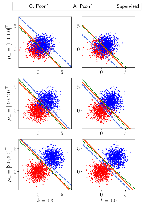
Figure 1: The visual illustrations of the impact of the different degrees of class overlap and skewed confidence. The red and blue points represent the positive and negative samples, respectively. The decision boundaries of original Pconf, adjusted Pconf and fully-supervised classification are shown as the blue, green and red lines, respectively.

4.1.1 Impact of Degree of Class Overlap and Skewed Confidence

We first examine the impact of the degree of class overlap and skewed confidence on the behaviour of Pconf classification. We fixed the mean of the positive distribution $\bm{\mu}_{+}$ to $\left[0,0\right]^{\top}$, and moved the mean of the negative distribution $\bm{\mu}_{-}$ from $\left[1.0,1.0\right]^{\top}$ to $\left[3.0,3.0\right]^{\top}$. We used the identity covariance for both the positive and negative distributions. In addition, we changed the degree of skewed confidence $b\in\left\{0.3,0.5,2.0,4.0\right\}$. We calculated the mean false negative (FN) rate over 10 trials with fully-supervised classification as $\widehat{\phi}$ (an estimate of $\phi$).

The mean and standard deviation of the classification accuracy over 10 trials are reported in Table 1. Adjusted Pconf worked well with all the candidates of the degree of class overlap and skewed confidence. It was statistically significantly better than original Pconf in all the cases, but difference in accuracy got smaller as the negative distribution moved away from the positive distribution. This result indicates that skewed confidence has less impact on problems where two distributions are easily separable because a small change of a decision boundary does not affect the classification result in such a situation. The visual illustrations of the results are presented in Figure 1.

4.1.2 Impact of Estimation Error of $\phi$

In the first experiment, we assumed that we had access to a precise estimate of the misclassification rate of positive samples $\phi$. However, this assumption would not always hold in practice. We then conducted the experiments with different values of $\widehat{\phi}$ to see the robustness of our proposed method against the estimation error of $\phi$. We used the mean FN rate reported in Table 1 multiplied by $c\in\left\{0.5,0.7,1.3,1.5\right\}$ as $\widehat{\phi}$ with estimation error.

Table 2 presents the results where $b=0.3$ and $4.0$. Although the classification accuracy decreased compared to the case with no estimation error in $\phi$, the decrease in accuracy was insignificant in some cases. Additionally, the accuracy of adjusted Pconf in Table 2 was better than the accuracy of original Pconf reported in Table 1 even for the cases with 50% estimation error ($c=0.5$ and $1.5$). This result demonstrates the usefulness of our proposed method in a practical situation where the value of $\phi$ cannot be precisely estimated.

Table 2: The mean and standard deviation of the classification accuracy over 10 trials using $\widehat{\phi}$ with estimation error. Bold face shows that the result is comparable to the case where $c=1.0$ (no error) according to the paired $t$-test at the significance level of 5%.

$b$	$\bm{\mu}_{-}$	$c=0.5$	$c=0.7$	$c=1.3$	$c=1.5$
0.3	1.0	73.08 $\pm$ 0.98	74.94 $\pm$ 0.87	75.30 $\pm$ 0.93	74.94 $\pm$ 0.64
	1.5	83.44 $\pm$ 0.95	84.72 $\pm$ 1.03	85.22 $\pm$ 0.77	84.75 $\pm$ 1.03
	2.0	90.81 $\pm$ 0.94	91.78 $\pm$ 0.71	91.70 $\pm$ 0.50	91.46 $\pm$ 0.52
	2.5	95.30 $\pm$ 0.99	95.80 $\pm$ 0.60	95.90 $\pm$ 0.42	95.74 $\pm$ 0.48
	3.0	98.06 $\pm$ 0.60	98.21 $\pm$ 0.56	98.30 $\pm$ 0.25	98.19 $\pm$ 0.19
4.0	1.0	73.84 $\pm$ 0.66	75.39 $\pm$ 0.58	75.40 $\pm$ 0.69	74.9 $\pm$ 0.76
	1.5	83.07 $\pm$ 0.58	84.55 $\pm$ 0.62	84.96 $\pm$ 1.00	84.60 $\pm$ 1.02
	2.0	91.32 $\pm$ 0.67	91.86 $\pm$ 0.56	92.08 $\pm$ 0.49	91.72 $\pm$ 0.44
	2.5	95.73 $\pm$ 0.43	96.15 $\pm$ 0.30	96.14 $\pm$ 0.47	95.88 $\pm$ 0.55
	3.0	97.92 $\pm$ 0.54	98.17 $\pm$ 0.34	98.27 $\pm$ 0.42	98.19 $\pm$ 0.43

4.2 Benchmark Experiments

We conducted two benchmark experiments with deep neural network models to evaluate the performance of our proposed method on image datasets. The experimental setups were based on [Ishida et al., 2018].

4.2.1 Fashion-MNIST

The Fashion-MNIST dataset is a set of 28 $\times$ 28 gray-scale images each of which represents one of the following 10 fashion item classes: T-shirt/top, pullover, dress, coat, sandal, shirt, sneaker, bag, and ankle boot. Each class consists of 7,000 images. We chose T-shirt/top as the positive class and one of the others as the negative class to construct a dataset for binary classification. We then divided it into four stratified sub-datasets: a training set, a validation set, a test set, and a dataset for estimating confidence.

We compared the performance of original Pconf classification, adjusted Pconf classification and fully-supervised classification. Skewed confidence was used for training both original and adjusted Pconf classifiers. We also included in this experiment original Pconf classification with non-skewed confidence to evaluate the performance decline caused by skew in confidence. The logistic loss was used for all of these methods.

We used a three-layer fully-connected neural network (784-100-100-1) with ReLU [Nair and Hinton, 2010] as an activation function and $10^{-7}$ weight decay. Optimization was executed by Adam [Kingma and Ba, 2015] for 200 epochs with minibatch size 100.

We generated positive confidence from a neural network with a softmax output layer and the same architecture as the aforementioned binary classifiers, but we used 50% dropout [Srivastava et al., 2014] after each fully-connected layer instead of weight decay. Additionally, we set the number of epochs to 20 in order to prevent the probabilistic output from being too close to 0 or 1, which is not suitable for the representation of confidence. We made confidence skewed by removing 90% negative samples from a dataset for training a softmax network. As a result, the dataset became imbalanced (P : N = 10 : 1), and confidence was skewed towards the positive class. Confidence lower than 0.01 was rounded up to 0.01 to stabilize the optimization. We used the mean FN rate over 20 trials with fully-supervised classification as an estimate of $\phi$.

The mean and standard deviation of the classification accuracy over 20 trials are reported in Table 3. Although skewed confidence severely affected the performance of original Pconf, it performed well with the accuracy over 90% in some cases where the supervised method had relatively high accuracy. This result was consistent with the synthetic experiment. Adjusted Pconf outperformed original Pconf in most of the cases, and was even competitive with fully-supervised classification and original Pconf with non-skewed confidence in some cases.

Table 3: The mean and standard deviation of the classification accuracy over 20 trials using three-layer fully-connected neural network models on the Fashion-MNIST dataset. Adjusted Pconf classification was compared with original Pconf classification, original Pconf classification with non-skewed confidence, and fully-supervised classification. We used the T-shirt/top as the positive class in all cases. Bold face denotes the best and comparable methods according to the paired $t$-test at the significance level of 5% between original Pconf and adjusted Pconf.

Negative	O. Pconf	A. Pconf	Non-skewed	Supervised
trouser	65.30 $\pm$ 9.92	91.72 $\pm$ 1.85	95.64 $\pm$ 0.30	99.12 $\pm$ 0.13
pullover	50.00 $\pm$ 0.00	84.31 $\pm$ 2.04	96.31 $\pm$ 0.12	96.90 $\pm$ 0.29
dress	50.00 $\pm$ 0.00	72.27 $\pm$ 2.79	91.13 $\pm$ 0.25	95.81 $\pm$ 0.55
coat	50.02 $\pm$ 0.07	85.42 $\pm$ 1.70	97.02 $\pm$ 0.19	98.61 $\pm$ 0.26
sandal	93.76 $\pm$ 10.41	96.42 $\pm$ 2.28	98.02 $\pm$ 0.84	99.84 $\pm$ 0.04
shirt	50.00 $\pm$ 0.00	70.12 $\pm$ 2.88	81.76 $\pm$ 0.14	85.21 $\pm$ 0.70
sneaker	97.66 $\pm$ 2.04	98.93 $\pm$ 0.13	97.48 $\pm$ 10.56	99.94 $\pm$ 0.04
bag	71.03 $\pm$ 10.88	92.28 $\pm$ 1.71	96.87 $\pm$ 0.17	98.86 $\pm$ 0.12
ankle boot	90.50 $\pm$ 11.06	99.22 $\pm$ 0.23	97.39 $\pm$ 1.33	99.92 $\pm$ 0.12

4.2.2 CIFAR-10

The CIFAR-10 dataset consists of 60,000 images in the $32\times 32\times$ RGB format. It includes 10 classes: airplane, automobile, bird, cat, deer, dog, frog, horse, ship, and truck. We chose airplane as the positive class and preprocessed the original dataset in the same way as the experiment with the Fashion-MNIST dataset.

In this experiment, we used a convolutional neural network model with the following architecture:

• Convolution (3 in- /18 out-channels, kernel size 5).

• Max-pooling (kernel size 2, stride 2).

• Convolution (18 in- /48 out-channels, kernel size 5).

• Max-pooling (kernel size 2, stride 2).

• Fully-connected (800 units) with ReLU.

• Fully-connected (400 units) with ReLU.

• Fully-connected (1 unit).

The results of the CIFAR-10 experiment are shown in Table 4. Adjusted Pconf outperformed original Pconf in all cases. Although the accuracy of adjusted Pconf was significantly lower than that of the fully-supervised method, adjusted Pconf was comparable to original Pconf with non-skewed confidence in some cases.

Table 4: The mean and standard deviation of the classification accuracy over 20 trials using convolutional neural network models on the CIFAR-10 dataset. Adjusted Pconf classification was compared with original Pconf classification, original Pconf classification with non-skewed confidence, and fully-supervised classification. We used the airplane as the positive class in all cases. Bold face denotes the best and comparable methods according to the paired $t$-test at the significance level of 5% between original Pconf and adjusted Pconf.

Negative	O. Pconf	A. Pconf	Non-skewed	Supervised
automobile	68.36 $\pm$ 6.27	79.66 $\pm$ 2.71	82.68 $\pm$ 0.76	93.35 $\pm$ 0.48
bird	68.42 $\pm$ 4.12	80.78 $\pm$ 1.67	82.29 $\pm$ 1.15	88.73 $\pm$ 0.66
cat	76.44 $\pm$ 7.16	85.08 $\pm$ 2.86	86.57 $\pm$ 1.02	92.35 $\pm$ 0.37
deer	74.16 $\pm$ 8.69	84.87 $\pm$ 2.30	86.71 $\pm$ 0.50	92.95 $\pm$ 0.52
dog	77.07 $\pm$ 6.24	85.28 $\pm$ 4.19	88.97 $\pm$ 1.51	94.24 $\pm$ 0.30
frog	83.62 $\pm$ 4.16	89.07 $\pm$ 1.28	90.34 $\pm$ 0.79	94.98 $\pm$ 0.38
horse	67.03 $\pm$ 9.75	77.02 $\pm$ 8.29	86.18 $\pm$ 1.02	94.68 $\pm$ 0.35
ship	57.55 $\pm$ 3.74	69.00 $\pm$ 1.98	69.87 $\pm$ 1.45	88.43 $\pm$ 0.50
truck	70.11 $\pm$ 4.15	81.25 $\pm$ 1.25	83.01 $\pm$ 0.88	90.85 $\pm$ 0.44

5 Real-World Application

In this section, we apply original and adjusted Pconf classification to the real-world problem of drivers’ drowsiness prediction. Through the experiment, we show that the confidence may be skewed in a real scenario, and can be corrected by our proposed method.

The objective of this application is to predict drivers’ drowsiness from the heartbeat information. Typically, a classifier for this problem can be trained with an experimental dataset including both Alert and Drowsy states collected by using a driving simulator. However, there are two issues with this way of building a classifier. The first one is derived from the fact that a driver reacts differently to a driving simulator and the real road situation [Hallvig et al., 2013]. A classifier trained with data from a driving simulator experiment may be less useful in the real traffic environment, but an experiment in the real environment is difficult and dangerous because drowsy driving easily leads to accidents. The second one is that driving until feeling strong drowsiness and the manual annotation of drivers’ states are extremely time-consuming even though we use a driving simulator. For these two issues, there is a strong motivation to learn a binary classifier without collecting Drowsy samples.

5.1 Drivers’ Drowsiness Dataset

We used an in-house drivers’ drowsiness dataset [Kaji et al., 2018], which was constructed from the driving simulator experiment. Three healthy males engaged in the driving task with a driving simulator along an expressway around 100 km/h overtaking other cars if necessary. The task continued until the strong drowsiness was observed or a driver finished the whole course (about 150 km). The facial expressions and the electrocardiogram (ECG) signal were recorded during the driving task to construct the dataset which includes the feature vector $\bm{x}$ and the drowsiness score $D$. The feature vector $\bm{x}$ was composed of seven heart-rate-variability indicators computed in the frequency domain (the spectral power of the low frequency component, etc) and time domain (the variance of the peak-to-peak interval of the R-wave, which is the largest wave of ECG, etc.). These features were computed at 60 seconds intervals with 120-second sliding windows, and normalized to have zero mean and unit standard deviation for each driver. Expert $j$ ($j=1,2,3$) independently evaluated the drowsiness score $D_{j}$ , which was rated from 1 (“Not sleepy”) to 5 (“Very sleepy”), based on the recorded facial expressions [Kitajima et al., 1997] every 60 seconds.

Each driver performed the driving tasks 10 times, and only five trials were annotated and the remaining five trials were unlabeled. We used the annotated five trials in this study.

5.2 Experimental Setup

We divided the collected data into Alert (positive) and Drowsy (negative) classes to reframe the drowsiness prediction as a binary classification problem. The samples with the median of the drowsiness score $D_{j}$ less than 3 were labeled as Alert, otherwise the samples were labeled as Drowsy. We also calculated the positive confidence from the drowsiness score $D_{j}$ as follows, which is confined between 0 and 1:

$$r=1-\frac{1}{12}\sum_{j=1}^{3}\left(D_{j}-1\right).$$

We compared the performance of original Pconf classification, adjusted Pconf classification, and fully-supervised classification. The logistic regression with the Gaussian kernel of bandwidth 1.0 was used for all of these methods.

In this experiment, the evaluation of the classification performance was conducted independently for each driver. More specifically, the samples of four driving trials by the same driver were used for training a classifier, and the samples of the remaining one trial were used as a test set. We repeated this procedure five times for each driver so that all trials were tested once. The F-measure was used as the performance metric since the dataset was imbalanced.

We computed the mean FN rate over 20 trials with fully-supervised classification for each driver, and then used the average of the mean FN rate of two drivers as an estimate of $\phi$ for the remaining one driver. Only Alert samples and their confidence were used for training original Pconf and adjusted Pconf classifiers, and hyperparameter tuning.

5.3 Results and Discussion

The results are reported in Table 5. The F-measure could not be calculated for original Pconf because it predicted all the samples to be Alert. This result suggests that there existed strong skew towards the Alert class in the confidence. It can be explained by the fact that it is difficult even for the experts to find out the sign of drowsiness on driver’s face because how the facial expressions change when she gets sleepy varies across drivers. Consequently, the drowsiness score tends to be lower than the actual drowsiness of drivers. Such bias can arise in any situation where there is asymmetric difficulty in evaluating confidence.

On the other hand, adjusted Pconf worked reasonably well with the drowsiness dataset. This result indicates that our method is also effective for the real-world problem where the positive confidence is given based on the subjective rating.

Table 5: The mean and standard deviation of the F-measure over 20 trials using kernel models on the drivers’ drowsiness dataset. Adjusted Pconf classification was compared with original Pconf classification, and fully-supervised classification. N/A indicates that the F-measure could not be calculated since the output was Alert (positive) for all the test samples.

Driver	O. Pconf	A. Pconf	Supervised
1	N/A	68.37 $\pm$ 0.96	59.92 $\pm$ 2.49
2	N/A	48.86 $\pm$ 0.50	66.29 $\pm$ 1.68
3	N/A	50.86 $\pm$ 0.87	55.66 $\pm$ 5.33

6 Conclusion

In this paper, we proposed adjusted Pconf classification to mitigate the influence of skewed confidence, which is not easy to handle but naturally emerges in the real-world applications. The key idea is the assumption of the misclassification rate of positive samples, which is minimal statistical information as a prior knowledge. The hyperparameter to correct skew in confidence is optimized through the minimization of the squared difference between the misclassification rate and validation error. We demonstrated the effectiveness of the proposed method through the synthetic and benchmark experiments, and the real-world drowsiness prediction problem.

References

- [Akiba et al., 2019] Takuya Akiba, Shotaro Sano, Toshihiko Yanase, Takeru Ohta, and Masanori Koyama. Optuna: A next-generation hyperparameter optimization framework. In KDD, 2019.
- [AlHanai and Ghassemi, 2017] Tuka Waddah AlHanai and Mohammad Mahdi Ghassemi. Predicting latent narrative mood using audio and physiologic data. In AAAI, 2017.
- [Bao and Intille, 2004] Ling Bao and Stephen Intille. Activity recognition from user-annotated acceleration data. In International Conference on Pervasive Computing, 2004.
- [Bao et al., 2018] Han Bao, Gang Niu, and Masashi Sugiyama. Classification from pairwise similarity and unlabeled data. In ICML, 2018.
- [Chapelle and Zien, 2005] Olivier Chapelle and Alexander Zien. Semi-supervised classification by low density separation. In AISTATS, 2005.
- [Chapelle et al., 2010] Olivier Chapelle, Bernhard Schlkopf, and Alexander Zien. Semi-Supervised Learning. The MIT Press, 2010.
- [Cour et al., 2011] Timothee Cour, Ben Sapp, and Ben Taskar. Learning from partial labels. Journal of Machine Learning Research, 12:1501–1536, 2011.
- [Dietterich et al., 1997] Thomas G. Dietterich, Richard H. Lathrop, and Tomas Lozano-Perez. Solving the multiple instance problem with axis-parallel rectangles. Artificial Intelligence, 89(1-2):31–71, 1997.
- [du Plessis and Sugiyama, 2013] Marthinus C. du Plessis and Masashi Sugiyama. Clustering unclustered data: Unsupervised binary labeling of two datasets having different class balances. In TAAI, 2013.
- [du Plessis et al., 2014] Marthinus C. du Plessis, Gang Niu, and Masashi Sugiyama. Analysis of learning from positive and unlabeled data. In NeurIPS. 2014.
- [Elkan and Noto, 2008] Charles Elkan and Keith Noto. Learning classifiers from only positive and unlabeled data. In KDD, 2008.
- [Hachisuka et al., 2011] Satori Hachisuka, Kenji Ishida, Takeshi Enya, and Masayoshi Kamijo. Facial expression measurement for detecting driver drowsiness. In Don Harris, editor, Engineering Psychology and Cognitive Ergonomics, pages 135–144. Springer, 2011.
- [Hallvig et al., 2013] David Hallvig, Anna Anund, Carina Fors, Göran Kecklund, Johan G. Karlsson, Mattias Wahde, and Torbjörn Åkerstedt. Sleepy driving on the real road and in the simulator—A comparison. Accident Analysis & Prevention, 50:44–50, 2013.
- [Horne and Reyner, 1999] Jim Horne and Louise Reyner. Vehicle accidents related to sleep: A review. Occupational and environmental medicine, 56:289–94, 1999.
- [Ishida et al., 2017] Takashi Ishida, Gang Niu, Weihua Hu, and Masashi Sugiyama. Learning from complementary labels. In NeurIPS, 2017.
- [Ishida et al., 2018] Takashi Ishida, Gang Niu, and Masashi Sugiyama. Binary classification from positive-confidence data. In NeurIPS. 2018.
- [Kaji et al., 2018] Hirotaka Kaji, Hayato Yamaguchi, and Masashi Sugiyama. Multi task learning with positive and unlabeled data and its application to mental state prediction. In ICASSP, 2018.
- [Kaji et al., 2019] Hirotaka Kaji, Hisashi Iizuka, and Masashi Sugiyama. ECG-based concentration recognition with multi-task regression. IEEE Transactions on Biomedical Engineering, 66(1):101–110, 2019.
- [Kato et al., 2019] Masahiro Kato, Takeshi Teshima, and Junya Honda. Learning from positive and unlabeled data with a selection bias. In ICLR, 2019.
- [Kingma and Ba, 2015] Diederik P. Kingma and Jimmy Ba. Adam: A method for stochastic optimization. In ICLR, 2015.
- [Kitajima et al., 1997] Hiroki Kitajima, Nakaho Numata, Keiichi Yamamoto, and Yoshihiro Goi. Prediction of automobile driver sleepiness (1st report, rating of sleepiness based on facial expression and examination of effective predictor indexes of sleepiness). Transactions of the Japan Society of Mechanical Engineers. C, 63(613):3059–3066, 1997.
- [Lane et al., 2014] Nicholas D. Lane, Mu Lin, Mashfiqui Mohammod, Xiaochao Yang, Hong Lu, Giuseppe Cardone, Shahid Ali, Afsaneh Doryab, Ethan Berke, Andrew T. Campbell, and Tanzeem Choudhury. Bewell: Sensing sleep, physical activities and social interactions to promote wellbeing. Mobile Networks and Applications, 19(3):345–359, 2014.
- [Liu and Tao, 2016] Tongliang Liu and Dacheng Tao. Classification with noisy labels by importance reweighting. IEEE Transactions on Pattern Analysis and Machine Intelligence, 38(3):447–461, 2016.
- [Liu et al., 2018] Bin Liu, Ying Li, Zhaonan Sun, Soumya Ghosh, and Kenney Ng. Early prediction of diabetes complications from electronic health records: A multi-task survival analysis approach. In AAAI, 2018.
- [Lu et al., 2019] Nan Lu, Gang Niu, Aditya K. Menon, and Masashi Sugiyama. On the minimal supervision for training any binary classifier from only unlabeled data. In ICLR, 2019.
- [Matthews et al., 2014] Mark Matthews, Saeed Abdullah, Geri Gay, and Tanzeem Choudhury. Tracking mental well-being: Balancing rich sensing and patient needs. Computer, 47(4):36–43, 2014.
- [Mintz et al., 2009] Mike Mintz, Steven Bills, Rion Snow, and Daniel Jurafsky. Distant supervision for relation extraction without labeled data. In ACL, 2009.
- [Nair and Hinton, 2010] Vinod Nair and Geoffrey Hinton. Rectified linear units improve restricted boltzmann machines. In ICML, 2010.
- [Natarajan et al., 2013] Nagarajan Natarajan, Inderjit S. Dhillon, Pradeep K. Ravikumar, and Ambuj Tewari. Learning with noisy labels. In NeurIPS. 2013.
- [Pedregosa et al., 2011] Fabian Pedregosa, Gaël Varoquaux, Alexandre Gramfort, Vincent Michel, Bertrand Thirion, Olivier Grisel, Mathieu Blondel, Peter Prettenhofer, Ron Weiss, Vincent Dubourg, Jake Vanderplas, Alexandre Passos, David Cournapeau, Matthieu Brucher, Matthieu Perrot, and Édouard Duchesnay. Scikit-learn: Machine learning in Python. Journal of Machine Learning Research, 12:2825–2830, 2011.
- [Sakai et al., 2017] Tomoya Sakai, Marthinus C. du Plessis, Gang Niu, and Masashi Sugiyama. Semi-supervised classification based on classification from positive and unlabeled data. In ICML, 2017.
- [Scholkopf and Smola, 2001] Bernhard Scholkopf and Alexander J. Smola. Learning with Kernels: Support Vector Machines, Regularization, Optimization, and Beyond. MIT Press, 2001.
- [Shinoda et al., 2019] Kazuhiko Shinoda, Masahiko Yoshii, Hayato Yamaguchi, and Hirotaka Kaji. Daytime sleepiness level prediction using respiratory information. In IJCAI, 2019.
- [Srivastava et al., 2014] Nitish Srivastava, Geoffrey Hinton, Alex Krizhevsky, Ilya Sutskever, and Ruslan Salakhutdinov. Dropout: A simple way to prevent neural networks from overfitting. The journal of machine learning research, 15(1):1929–1958, 2014.
- [Vural et al., 2007] Esra Vural, Mujdat Cetin, Aytul Ercil, Gwen Littlewort, Marian Bartlett, and Javier Movellan. Drowsy driver detection through facial movement analysis. In Michael Lew, Nicu Sebe, Thomas S. Huang, and Erwin M. Bakker, editors, Human–Computer Interaction, pages 6–18. Springer, 2007.
- [Weiss et al., 2016] Gary M. Weiss, Jeffrey W. Lockhart, Tony T. Pulickal, Paul T. McHugh, Isaac H. Ronan, and Jessica L. Timko. Actitracker: A smartphone-based activity recognition system for improving health and well-being. In IEEE International Conference on Data Science and Advanced Analytics, pages 682–688, 2016.
- [Zhou, 2018] Zhi-Hua Zhou. A brief introduction to weakly supervised learning. National Science Review, 5(1):44–53, 2018.
- [Zhu et al., 2003] Xiaojin Zhu, Zoubin Ghahramani, and John Lafferty. Semi-supervised learning using gaussian fields and harmonic functions. In ICML, 2003.