Automatic weak imposition of free slip boundary conditions via Nitsche’s method: application to nonlinear problems in geodynamics

Abstract

Imposition of free slip boundary conditions in science and engineering simulations presents a challenge when the simulation domain is non-trivial. Inspired by recent progress in symbolic computation of discontinuous Galerkin finite element methods, we present a symmetric interior penalty form of Nitsche’s method to weakly impose these slip boundary conditions and present examples of its use in the Stokes subsystem motivated by problems in geodynamics. We compare numerical results with well established benchmark problems. We also examine performance of the method with iterative solvers.
Keywords: Finite element analysis, symbolic computational methods, parallel and high-performance computing, mantle convection, subduction zone modelling, geodyanmics.

1 Introduction

This work is born of a common question asked of the authors. Regarding engineering and geodynamics finite element analysis, how does one implement free slip boundary conditions? In particular, the case that the geometry is a non-trivial shape such as that representative of a ‘real–world problem’. Typically the author’s recommendation is to use Nitsche’s method. However, this recommendation is met with trepidation regarding the difficulty of implementation in addition to a reputation for not performing well with iterative solvers.

The intent of this work to dispel these concerns. Specifically by providing the mathematical and open source user-friendly software tools to compute finite element problems using Nitsche’s method for (but not limited to) incompressible flow simulations. Additionally by providing numerical examples which demonstrate the viability of Nitsche’s method for the imposition of free slip boundary data in geodynamics problems.

1.1 Nitsche’s method

Nitsche’s original work [32] proposed a method for the weak imposition of Dirichlet boundary conditions on the exterior of a computational domain. The term ‘weak imposition’ implies that the Dirichlet boundary condition is not applied as a modification of the underlying finite element linear algebra system (strong imposition), but rather as a component of the variational formulation. These additional terms in the variational formulation comprise exterior facet integrals penalising the difference between the (unknown) finite element solution and the boundary condition data, and enforcing consistency and coercivity according to the underlying weak formulation.

Enforcing boundary conditions in this variational setting permits additional flexibility. For example, Nitsche’s method could be used to enforce inequalities on the boundary such as that required by the Signorini problem [15, 45]. Furthermore, Nitsche’s method is exploitable in pseudo arc–length continuation of boundary condition parameters given that the underlying finite element matrix need not be manipulated [1]. Recently Nitsche’s method has found popularity for problems with complex geometries by immersion in a background mesh using the CutFEM technique [14]. In this paper we exploit this flexibility for the imposition of free slip boundary data. Specifically, given a computational domain, the free slip boundary condition requires that the component of the unknown vector valued solution which acts parallel to the domain boundary’s normal vector must vanish.

1.2 Strong and weak imposition of the free slip condition

1.2.1 Strong imposition

The strong imposition of free slip boundary data is trivial when the exterior boundary of the computational domain aligns with the coordinate system. In this case, one of the orthogonal components of the vector valued solution may be strongly enforced to vanish, while the other components are solved in a natural sense.

In the case of non-trivial geometries strong imposition is no longer so straightforward. The underlying finite element stiffness matrix, $\mathrm{A}$, must be manipulated such that degrees of freedom associated with the vector valued solution are constrained in the boundary normal direction. For example, consider the unknown solution vector $\mathrm{u}$, constraint matrix $\mathrm{C}$ and load vector $\mathrm{b}$, the finite element system becomes: find $\mathrm{u}$ such that

$$\mathrm{C^{\top}ACu}=\mathrm{C^{\top}b},$$ (1)

where the prefactor $\mathrm{C}^{\top}$ preserves symmetry. The matrix product operation on the left hand side of eq. 1 is computationally expensive. Therefore the operator $\widehat{\mathrm{A}}=\mathrm{C^{\top}AC}$ should be assembled directly when constructing the finite element system.

When imposing free slip boundaries in a strong sense, we must also take into account that the outward pointing unit normal vector on the boundary is not well defined for all finite elements. Consider a vector valued solution sought in a standard piecewise linear finite element vector space. The degrees of freedom are defined at the vertices of the mesh. At these degrees of freedom the facet normal is not well defined, see fig. 1 for example. Special treatment of these cases could be considered by, for example, taking the average of the two neighbouring facets. However, what approach should be taken at the intersection of three or more boundaries? This requirement presents itself in a numerical example shown later in section 5.4.

The implementation challenge for strong imposition lies in the efficient assembly of $\widehat{\mathrm{A}}$, the clear definition of the facet normal, and a user–friendly interface for the definition of boundary conditions generating $\mathrm{C}$, cf. [11].

1.2.2 Lagrange multiplier

Another approach to the imposition of free slip boundary data is by Langrange multiplier. In this setting a new Langrage multiplier variable is introduced to enforce the free slip boundary data as a system constraint in the variational formulation. This mathematical setting provides a flexible framework for the imposition of boundary data, however, the expanded variational formulation causes the underlying linear system to the grow by an additional block row and column. Additionally this block must be carefully considered when preconditioning the underlying linear system. We refer to [41] for a summary of the use of Lagrange multiplier methods for free slip boundary data in the Stokes system.

1.2.3 Nitsche’s method

Nitsche’s method is attractive for free slip boundary conditions. The normal and tangential components of the vector field on each boundary can be separated and prescribed in a mathematically consistent setting [32, 41, 5]. Specifically without the need for definition of a facet normal at mesh vertices. There is no requirement for the constraint matrix $\mathrm{C}$ to be constructed. Simply assembly of the stiffness matrix $\mathrm{A}$. And there is no requirement for growth in the block size of the underlying linear system, also simplifying preconditioning. The implementation challenge lies in a user–friendly interface for defining a boundary condition by Nitsche’s method. We address this in section 4.

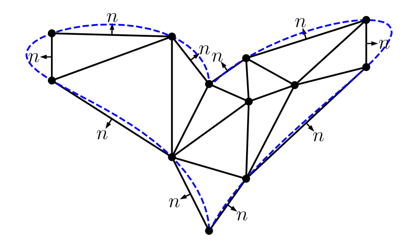
Figure 1: Example mesh discretisation using a piecewise linear boundary representation. The true boundary is indicated by the dashed line. $n$ denotes the outward pointing normal unit vector on the mesh exterior. The degrees of freedom of a standard piecewise linear finite element function space are defined at the vertices of the mesh. Consider how the facet normal is not defined at these locations which is problematic for strong imposition of free slip boundary conditions.

1.3 Geodynamics models

The conservation equations underlying geodynamics models typically encapsulate the Stokes system. In turn, these models require free slip boundary conditions, for example at the core-mantle-boundary and lithosphere [12, 40], or on a dipping slab in a subduction zone [42].

Prior works demonstrate the use of Nitsche’s method for the imposition of free slip velocities in the Stokes system in a linear setting [41, 30, 20, 21]. However, modern geodynamics simulations are concerned with highly nonlinear temperature and strain rate dependent viscosity models.

At this point, we highlight that the discontinuous Galerkin (DG) method can be considered a generalisation of Nitsche’s method. Drawing our attention to the DG literature, we find that imposition of free slip boundary conditions in nonlinear compressible flow problems is commonplace, for example [23]. Therefore we seek to marry the presentation of Nitsche’s method for the Stokes system with the works which examine the formulations of DG finite element method (FEM) for nonlinear problems.

Whilst doing this, we must ensure that the extra terms arising from Nitsche’s method will be formulated automatically and in a familiar and ‘friendly’ manner in the computational framework. Ultimately, the utility of Nitsche’s method in esoteric modelling is strongly dependent on its ease of use.

1.4 Implementation

A key detriment of Nitsche’s method is its difficulty to implement. In the case of a problem such as the finite element discretisation of Poisson’s equation, the additional facet integral terms are straightforward to add to a finite element code. However, for more complex systems such as hyperelasticity, incompressible and compressible flow and electromagnetics, the additional facet terms are verbose and prone to human error. Introducing nonlinear material coefficients (such as diffusivity or viscosity) yields a finite element formulation arduous to write on paper, let alone in code.

The challenge therefore presents itself. We seek to homogenise the mathematical formulation of Nitsche’s method for these classes of finite element problems. Thereby we construct a computational tool for automatically applying boundary conditions by Nitsche’s method, agnostic of the underlying finite element problem.

The former issue of homogenisation of the mathematical problem is demonstrated in works such as [23, 22, 25]. We repeat these formulations later in this work. Computational symbolic representation of the underlying finite element formulation is used to address the latter issue for constructing a computational tool. In this setting the finite element formulation is represented in computer code which is intended to be high-level, familiar and recognisible from the mathematical formulation. From this representation high performance code for the assembly of the finite element matrix and vector is automatically generated. In this vein, a particularly popular open source framework is the Unified Form Language (UFL) [2]. For example, UFL has been adopted by the following open source finite element suites: FEniCS and FEniCS–X (used in this work) [3, 19], the Firedrake project [33], DUNE-FEM [17] and TerraFERMA [44]. Other projects have developed their own framework for automatic code generation, for example FreeFem++ [24], NGSolve [37] and AptoPy/FEM [38].

Despite the advantages of the computational symbolic algebra representation, the implementation of Nitsche exterior facet terms is still verbose and prone to human error. Houston and Sime’s prior work with automatic symbolic formulation of DG methods addresses this issue in the development of the dolfin_dg library [25]. They demonstrate how finite element packages with computational symbolic representation of the variational formulation can be exploited to add another layer of abstraction by automatically generating the DG finite element formulation itself.

The paradigm of automatic finite element formulation–formulation will be exploited here. The strong similarity between the weak imposition of exterior Dirichlet boundary conditions by the DG finite element method and Nitsche’s method allow us to use the designs exhibited in [25].

1.5 Iterative solvers

Although the automatic formulation of the Nitsche terms in the weak formulation is useful, the generated code for assembling the finite element system must perform well. For example, many modern geodynamics models require discretisations of equations defined in complex 3D geometries. Meshes of these geometries must be of sufficient granularity and fidelity which give rise to very large numbers of unknowns.

The FEniCS and FEniCS–X finite element software is used in this work. It has been demonstrated to be scalable when solving large systems where the degree of freedom count exceeds ${10}^{9}$ [34, 35]. Therefore we seek to ensure that the use of automatically generated Nitsche terms does not impact this scaling.

A key component of scalable finite element analysis is the use of iterative solvers. For example Krylov subspace solvers combined with algebraic multigrid preconditioners. The standard Nitsche term which penalises the difference between the unknown solution and the boundary data incorporates a penalty parameter. Indeed, those unfamiliar with Nitsche’s method may recognise the penalty method when ignoring the consistency and coercivity terms. However, the penalty method’s penalty parameter would typically be a large number which can be detrimental to the condition number of the underlying finite element matrix. In turn this could impact the utility of iterative methods causing Krylov methods to stagnate or diverge [36]. By use of Nitsche’s method, this penalty parameter may be orders of magnitude smaller, yielding a (typically) well conditioned linear system ripe for solution by exploiting iterative methods [27]. This is explored in the ultimate numerical example of this paper in section 5.5.

1.6 Article outline

The flow of this paper is as follows: In section 2.3 we form a foundation of Nitsche’s method for Dirichlet boundary data in a general sense for elliptical partial differential equation (PDE) problems. The specialised case for Dirichlet boundary data in a direction perpendicular to a domain’s boundary is presented in section 2.4. With this foundation we formulate the Boussinesq approximation in section 3 in addition to free slip boundary conditions and thereby its finite element formulation. We highlight the benefits of the automatic formulation of the Nitsche boundary terms using computational symbolic algebra by the UFL and dolfin_dg libraries in section 4. With all the tools in place, we demonstrate numerical experiments in section 5. Finally we provide some concluding remarks in section 6.

2 Weak imposition of the slip boundary condition

In this section we examine the formulation of Nitsche’s method in a general setting for nonlinear elliptic problems. Initially in section 2.1 we define the general nonlinear elliptic equation. Inspired by the DG FEM literature, a symmetric interior penalty Galerkin (SIPG) approach will be taken [5] while noting here that we are not limited to solely the SIPG formulation. In section 2.3 the general formulation of the weak imposition of Dirichlet data on the exterior boundary is presented as summarised in prior work [25]. Using this as a foundation, we then focus on the case that normal and tangential data should be prescribed separately in section 2.4. This yields the semilinear formulation for imposition of the free slip boundary condition.

2.1 Elliptic nonlinear boundary value problem

Let $\Omega\subset\mathbb{R}^{d}$, $d=2,3$, be the domain of interest, e.g. the Earth’s mantle. The boundary of the domain is $\partial\Omega=\Gamma$ which is subdivided into Dirichlet, Neumann and ‘slip’ components, $\Gamma_{D}$, $\Gamma_{N}$ and $\Gamma_{S}$, respectively. By ‘slip’ boundary we mean that the normal and tangential components are prescribed in the Dirichlet and Neumann sense, respectively, on $\Gamma_{S}$. The boundary components do not overlap $\Gamma_{D}\cap\Gamma_{S}\cap\Gamma_{N}=\emptyset$ and the Dirichlet boundary must either be non-empty $\Gamma_{D}\neq\emptyset$ or the tangent of the ‘slip’ boundary must span at a minimum $d$ non–parallel planes. Let $n$ be unit vector pointing outward and normal to the boundary $\Gamma$.

The abstract nonlinear elliptic PDE of interest is to find $u$ such that:

$$-\nabla\cdot\mathcal{F}^{v}(u,\nabla u)=f\quad\text{ in }\Omega$$ (2)

complemented by boundary conditions

$$u =u_{D} \text{ on }\Gamma_{D},$$ (3)

$$\mathcal{F}^{v}(u,\nabla u)\cdot n =g_{N} \text{ on }\Gamma_{N},$$ (4)

$$u\cdot n =u_{S}\cdot n \text{ on }\Gamma_{S},$$ (5)

$$(\mathcal{F}^{v}(u,\nabla u)\cdot n)\cdot\tau_{i} =g_{\tau,i},\quad i=1,\ldots,d-1, \text{ on }\Gamma_{S},$$ (6)

where $u_{D}$, $g_{N}$, $u_{S}$ and $g_{\tau,i}$, $i=1,\ldots,d-1$, are Dirichlet, Neumann, normal Dirichlet and tangential Neumann data, respectively. $\tau_{i}$, $i=1,\ldots,d-1$, are the orthonormal vectors which span the plane tangential to $\Gamma_{S}$.

2.2 Finite element formulation

The domain $\Omega$ is subdivided into non-overlapping elements $\kappa$ of size $h_{\kappa}$. These elements comprise a mesh $\mathcal{T}^{h}=\cup_{\kappa}\kappa$. Let $V^{h,\ell}$ be the finite element space of piecewise polynomials defined on each element $\kappa\in\mathcal{T}^{h}$ of degree $\ell\in\mathbb{N}$ and continuous in $\Omega$. We use the notation $(u,v)=\int_{\Omega}u\cdot v\operatorname{d\!}{x}$ to define the inner product in $\Omega$, and on the exterior boundary $(u,v)_{\Gamma}=\int_{\Gamma}u\cdot v\operatorname{d\!}{s}$.

The finite element formulation of the system eq. 2 is to find $u_{h}\in V^{h,\ell}$ such that

$$\mathcal{N}(u_{h},v)\coloneqq\mathcal{N}_{\Omega}(u_{h},v)+\mathcal{N}_{\Gamma_{D}}(u_{h},v)+\mathcal{N}_{\Gamma_{N}}(u_{h},v)+\mathcal{N}_{\Gamma_{S}}(u_{h},v)\equiv 0\quad\forall v\in V^{h,\ell}.$$ (7)

Here the semilinear residual terms $\mathcal{N}_{\Omega}(\cdot,\cdot),\mathcal{N}_{\Gamma_{D}}(\cdot,\cdot),\mathcal{N}_{\Gamma_{N}}(\cdot,\cdot)$ and $\mathcal{N}_{\Gamma_{S}}(\cdot,\cdot)$ correspond to the volume, Nitsche Dirichlet, Neumann and Nitsche ‘slip’ boundary terms, respectively. Clearly at this stage we are able to define

$$\mathcal{N}_{\Omega}(u,v) \coloneqq(\mathcal{F}^{v}(u,\nabla u),\nabla v)-(f,v),$$ (8)

$$\mathcal{N}_{\Gamma_{N}}(u,v) \coloneqq-(g_{N},v)_{\Gamma_{N}}.$$ (9)

The remaining terms, $\mathcal{N}_{\Gamma_{D}}(\cdot,\cdot)$ and $\mathcal{N}_{\Gamma_{S}}(\cdot,\cdot)$ will be defined in the following sections.

2.3 Symmetric interior penalty Galerkin method for Dirichlet boundary data

In this section we will define $\mathcal{N}_{\Gamma_{D}}(\cdot,\cdot)$. We recall the SIPG method for the weak imposition of Dirichlet boundary data and refer to the review [5] and the monographs cited therein for details and analysis. For more details of the formulation presented in this section we refer to [25].

Firstly we homogenise eq. 2 such that

$$-\nabla\cdot\mathcal{F}^{v}(u,\nabla u)=-\nabla\cdot\mathinner{\left(G\nabla u\right)},$$ (10)

where $G$ is the homogenity tensor defined by

$$G_{kl}\coloneqq\frac{\partial\mathfrak{f}^{v}_{k}}{\partial\mathinner{\left(\nabla u\right)}_{l}},\quad k,l=1,\ldots,d,$$ (11)

which is written in terms of the columns of the viscous flux operator

$$\mathcal{F}^{v}(u,\nabla u)=(\mathfrak{f}^{v}_{1}(u,\nabla u),\ldots,\mathfrak{f}^{v}_{d}(u,\nabla u))$$ (12)

and we use the hyper-tensor product (in terms of Einstein summation notation)

$$(G\nabla u)_{ik}=(G_{kl})_{ij}(\nabla u)_{jl}.$$ (13)

Here, we are concerned only with applying the weak imposition of boundary data $u_{\Gamma}(u)=u_{D}$ on the Dirichlet boundary $\Gamma_{D}$. The Nitsche boundary formulation in terms of the homogeneity tensor is given by

$$\mathcal{N}_{\Gamma_{D}}(u,v)\coloneqq -\mathinner{\left(\mathcal{F}^{v}(u_{\Gamma},\nabla u),v\otimes n\right)}_{\Gamma_{D}}$$

$$-\mathinner{\left((u-u_{\Gamma})\otimes n,G^{\top}_{\Gamma}\nabla v\right)}_{\Gamma_{D}}$$

$$-C_{\mathrm{IP}}\frac{\ell^{2}}{h_{F}}\mathinner{\left(G_{\Gamma}(u-u_{\Gamma})\otimes n,v\otimes n\right)}_{\Gamma_{D}},$$ (14)

where $G_{\Gamma}=G(u_{\Gamma}(u))$ and the transpose product $(G^{\top}\nabla v)_{jl}=(G_{kl})_{ij}(\nabla v)_{ik}$, $h_{F}$ is the measure of the local facet $F$ which discretises $\partial\Omega$ and $C_{\mathrm{IP}}$ is a sufficiently large constant interior penalty parameter which is independent of the mesh chosen to be $C_{\mathrm{IP}}=20$ in this work [26].

2.4 SIPG-weak imposition of boundary data in the facet normal direction

The previous section provides a familiarity for the weak imposition of Dirichlet boundary data on $\Gamma_{D}$. Now consider that only the component of the numerical flux acting perpendicular to the boundary $\Gamma_{S}$ be prescribed. This leaves the remaining tangenital component on $\Gamma_{S}$ to be naturally enforced.

We define the normal projection and rejection operators acting on a vector $v\in\mathbb{R}^{d}$

$$P_{n}(v) \coloneqq(n\otimes n)\cdot v,$$ (15)

$$P_{\tau}(v) \coloneqq v-P_{n}(v)=(I-n\otimes n)\cdot v,$$ (16)

respectively. One can intuitively interpret $P_{n}(v)$ and $P_{\tau}(v)$ as the normal and tangential components of $v$, respectively. On $\Gamma_{S}$ the normal component of the numerical flux $\mathcal{F}^{v}(u,\nabla u)\cdot n$ needs to be conserved. This numerical flux is written in terms of normal and tangential components as follows

$$\mathcal{F}^{v}(u,\nabla u)\cdot n =P_{n}(\mathcal{F}^{v}(u,\nabla u)\cdot n)+P_{\tau}(\mathcal{F}^{v}(u,\nabla u)\cdot n)$$

$$=P_{n}(\mathcal{F}^{v}(u,\nabla u)\cdot n)+\sum_{i=1}^{d-1}g_{\tau,i}\tau_{i}.$$ (17)

Furthermore we note the following identity

$$(v\otimes n,\mathcal{F}^{v}(u,\nabla u))=(v_{i}n_{j},\mathcal{F}^{v}(u,\nabla u)_{ij})=(v_{i},\mathcal{F}^{v}(u,\nabla u)_{ij}n_{j})=(v,\mathcal{F}^{v}(u,\nabla u)\cdot n).$$ (18)

Applying eqs. 17 and 18 to the Nistche boundary terms in eq. 14 we arrive at the following integrals on the boundary $\Gamma_{S}$

$$\mathcal{N}_{\Gamma_{S}}(u,v)\coloneqq -\sum_{i=1}^{d-1}\mathinner{\left(g_{\tau,i},v\cdot\tau_{i}\right)}_{\Gamma_{S}}$$

$$-\mathinner{\left(P_{n}(\mathcal{F}^{v}(u_{\Gamma},\nabla u)\cdot n),v\right)}_{\Gamma_{S}}$$

$$-\mathinner{\left(u-u_{\Gamma},P_{n}((G^{\top}_{\Gamma}\nabla v)\cdot n)\right)}_{\Gamma_{S}}$$

$$-C_{\mathrm{IP}}\frac{\ell^{2}}{h_{F}}\mathinner{\left(P_{n}((G_{\Gamma}(u-u_{\Gamma}))\cdot n),v\right)}_{\Gamma_{S}}.$$ (19)

On $\Gamma_{S}$ the boundary flux function is set such that solely the normal component is prescribed data, i.e., $u_{\Gamma}(u)=u_{S}$.

3 Boussinesq approximation

With the general formulation eq. 2 and its finite element formulation eq. 7 and terms defined in eqs. 8, 9, 14 and 19 we move on to the specific case of the steady state incompressible Boussinesq approximation. The Boussinesq approximation underpins mantle convection simulations of buoyancy driven flow. We seek the non–dimensionalised velocity $u$, pressure $p$ and temperature $T$ such that equations for conservation of momentum, mass and energy are satisfied

$$-\nabla\cdot\left(2\eta\varepsilon(u)-pI\right) =f \text{ in }\Omega,$$ (20)

$$\nabla\cdot u =0 \text{ in }\Omega,$$ (21)

$$-\nabla\cdot\mathinner{\left(\kappa\nabla T\right)}+u\cdot\nabla T =Q \text{ in }\Omega.$$ (22)

Here $Q$ is an external heat source, $\varepsilon(u)=\frac{1}{2}(\nabla u+{\nabla u}^{\top})$ is the rate of strain tensor, $I_{ij}=\delta_{ij}$, $i,j=1,\ldots,d$, is the identity tensor, $f$ is a momentum source and $\eta$ is the viscosity. We highlight that the viscosity is typically a nonlinear function of the temperature and velocity, i.e., $\eta=\eta(u,T)$. This mandates that the system eqs. 20, 21 and 22 is nonlinear.

3.1 Stokes subsystem finite element formulation

We focus our attention on the Stokes subsystem in eqs. 20 and 21. Here $\mathcal{F}^{v}(u,\nabla u)=(2\eta\varepsilon(u)-pI)$. Discretising, the finite element formulation reads: find $(u_{h},p_{h},T_{h})\in W^{h}$ where $W^{h}$ is an appropriate mixed element such that

$$\mathcal{N}_{\text{Boussinesq}}(u_{h},p_{h};v_{h},q) \vcentcolon=\mathcal{N}_{\text{momentum}}(u_{h},p_{h},T_{h};v)$$

$$+\mathcal{N}_{\text{mass}}(u_{h},p_{h},T_{h};q)$$

$$+\mathcal{N}_{\text{energy}}(u_{h},p_{h},T_{h};s)\equiv 0$$

$$\quad\forall(v,q,s)\in W^{h}.$$ (23)

The formulations $\mathcal{N}_{\text{momentum}}$ and $\mathcal{N}_{\text{energy}}$ are formed from eqs. 20 and 22 in a straightforward manner according to eq. 7. The special case of the first order continuity formulation $\mathcal{N}_{\text{mass}}$ is given by

$$\mathcal{N}_{\text{mass}}(u,q)\coloneqq(\nabla\cdot u,q)-((u-u_{\Gamma})\cdot n,q)_{\Gamma_{D}\cup\Gamma_{S}},$$ (24)

see [16, 38], for example. Two choices of $W^{h}$ are employed in this work:

• The standard Taylor–Hood element where $W^{h,\text{TH}}=[V^{h,\ell}]^{d}\times V^{h,\ell-1}\times V^{h,\mathfrak{s}}$ and $\ell\geq 2$ and $\mathfrak{s}\geq 1$ [39].

• The suboptimal piecewise constant pressure approximation where $W^{h,0}=[V^{h,2}]^{d}\times V^{h,0}\times V^{h,\mathfrak{s}}$ and $\mathfrak{s}\geq 1$. See [6, 13] for example.

4 Implementation

Despite homogenisation, writing the code for the finite element system assembly of eq. 23 is made particularly difficult and verbose by the Nitsche boundary terms. The complexity of the implementation is spectacularly prone to human error. To combat this issue we represent the finite element formulation using the computational symbolic algebra package UFL [2]. Combined with the core components of the FEniCS and FEniCS-X projects [3, 19], this symbolic representation is then translated to high performance code for the assembly of the finite element system.

The UFL offers a much more straightforward method for generating finite element code of standard problems. However, the extra boundary terms found in eq. 23 are still verbose, even in this friendlier computational framework.

Prior work has shown the use of the FEniCS project for the automatic formulation of DG finite element formulations in the library dolfin_dg [25]. Given that the DG method can be considered a generalisation of Nitsche’s method, we can exploit the dolfin_dg library to automatically formulate and generate the code required by the Nitsche boundary terms.

We summarise the implementation details in this section, highlighting the benefits of the mathematical homogenisation we have shown in section 2. Python scripts will be shown to elucidate features specific for the formulation of the exterior integral terms. However, for a background of development and intricacies of the design philosophy we refer to [25].

4.1 Automatic finite element formulation–formulation using FEniCS and dolfin_dg

FEniCS and FEniCS-X provide a succinct way of describing and solving the Stokes system, see the many documented examples in [29]. We illustrate one case using a manufactured solution in LABEL:code:stokes_full. The full details of this case will be discussed in section 5.1. For now we note that it follows a standard FEniCS workflow; describing the mesh and geometry where ${n=\mbox{\leavevmode\lstinline{{\lst@@@set@language\lst@@@set@numbers\lst@@@set@frame\lst@@@set@rulecolor\lst@@@set@numbers\lst@@@set@frame\lst@@@set@language{\@listingGroup{ltx_lst_identifier}{n}}}}}}$, the finite element functionspace (here the lowest-order Taylor–Hood element) ${W^{h,\text{TH}}=[V^{h,2}]^{d}\times V^{h,1}=\mbox{\leavevmode\lstinline{{\lst@@@set@language\lst@@@set@numbers\lst@@@set@frame\lst@@@set@rulecolor\lst@@@set@numbers\lst@@@set@frame\lst@@@set@language{\@listingGroup{ltx_lst_identifier}{W}}}}}}$, and expressions for the known manufactured solution u_soln and p_soln, and an initial guess U for solution by Newton’s iterative method.

To describe the Stokes system, and weakly impose slip boundary conditions using Nitsche’s method, the crucial function to define is ${\mathcal{F}^{v}(u,\nabla u)=\mbox{\leavevmode\lstinline{{\lst@@@set@language\lst@@@set@numbers\lst@@@set@frame\lst@@@set@rulecolor\lst@@@set@numbers\lst@@@set@frame\lst@@@set@language{\@listingGroup{ltx_lst_identifier}{F\textunderscore v}}}}}}$:

⬇

def F_v(u, grad_u, p_local=None):

if p_local is None:

p_local = p

return 2 * eta(u) * sym(grad_u) - p_local * Identity(2)

doflin_dg requires this to have two arguments: ${u=\mbox{\leavevmode\lstinline{{\lst@@@set@language\lst@@@set@numbers\lst@@@set@frame\lst@@@set@rulecolor\lst@@@set@numbers\lst@@@set@frame\lst@@@set@language{\@listingGroup{ltx_lst_identifier}{u}}}}}}$ and ${\nabla u=\mbox{\leavevmode\lstinline{{\lst@@@set@language\lst@@@set@numbers\lst@@@set@frame\lst@@@set@rulecolor\lst@@@set@numbers\lst@@@set@frame\lst@@@set@language{\@listingGroup{ltx_lst_identifier}{grad\textunderscore u}}}}}}$. In this example it also depends on a function defining the viscosity ${\eta(u)=\mbox{\leavevmode\lstinline{{\lst@@@set@language\lst@@@set@numbers\lst@@@set@frame\lst@@@set@rulecolor\lst@@@set@numbers\lst@@@set@frame\lst@@@set@language{\@listingGroup{ltx_lst_identifier}{eta}}({\@listingGroup{ltx_lst_identifier}{u}})}}}}$ and the pressure ${p=\mbox{\leavevmode\lstinline{{\lst@@@set@language\lst@@@set@numbers\lst@@@set@frame\lst@@@set@rulecolor\lst@@@set@numbers\lst@@@set@frame\lst@@@set@language{\@listingGroup{ltx_lst_identifier}{p}}}}}}$.

The finite element solution variables ${u=\mbox{\leavevmode\lstinline{{\lst@@@set@language\lst@@@set@numbers\lst@@@set@frame\lst@@@set@rulecolor\lst@@@set@numbers\lst@@@set@frame\lst@@@set@language{\@listingGroup{ltx_lst_identifier}{u}}}}}}$ and ${p=\mbox{\leavevmode\lstinline{{\lst@@@set@language\lst@@@set@numbers\lst@@@set@frame\lst@@@set@rulecolor\lst@@@set@numbers\lst@@@set@frame\lst@@@set@language{\@listingGroup{ltx_lst_identifier}{p}}}}}}$ and respective test functions ${v=\mbox{\leavevmode\lstinline{{\lst@@@set@language\lst@@@set@numbers\lst@@@set@frame\lst@@@set@rulecolor\lst@@@set@numbers\lst@@@set@frame\lst@@@set@language{\@listingGroup{ltx_lst_identifier}{v}}}}}}$ and ${q=\mbox{\leavevmode\lstinline{{\lst@@@set@language\lst@@@set@numbers\lst@@@set@frame\lst@@@set@rulecolor\lst@@@set@numbers\lst@@@set@frame\lst@@@set@language{\@listingGroup{ltx_lst_identifier}{q}}}}}}$ corresponding to velocity and pressure are defined such that the variational formulation may be written. F_v is used to define the non-linear residual for the Stokes system ${\mathcal{N}_{\text{Stokes}}=\mathcal{N}_{\text{momentum}}+\mathcal{N}_{\text{mass}}=\mbox{\leavevmode\lstinline{{\lst@@@set@language\lst@@@set@numbers\lst@@@set@frame\lst@@@set@rulecolor\lst@@@set@numbers\lst@@@set@frame\lst@@@set@language{\@listingGroup{ltx_lst_identifier}{N}}}}}}$. We also use F_v to define the momentum source ${f=\mbox{\leavevmode\lstinline{{\lst@@@set@language\lst@@@set@numbers\lst@@@set@frame\lst@@@set@rulecolor\lst@@@set@numbers\lst@@@set@frame\lst@@@set@language{\@listingGroup{ltx_lst_identifier}{f}}}}}}$ and the tangential component of the Neumann boundary condition ${g_{\tau,1}=\mbox{\leavevmode\lstinline{{\lst@@@set@language\lst@@@set@numbers\lst@@@set@frame\lst@@@set@rulecolor\lst@@@set@numbers\lst@@@set@frame\lst@@@set@language{\@listingGroup{ltx_lst_identifier}{g\textunderscore tau}}}}}}$ based on the manufactured solution, where ${P_{\tau}(v)=\mbox{\leavevmode\lstinline{{\lst@@@set@language\lst@@@set@numbers\lst@@@set@frame\lst@@@set@rulecolor\lst@@@set@numbers\lst@@@set@frame\lst@@@set@language{\@listingGroup{ltx_lst_identifier}{tangential\textunderscore proj}}({\@listingGroup{ltx_lst_identifier}{v}},{\@listingGroup{ltx_lst_space}{ }}{\@listingGroup{ltx_lst_identifier}{n}})}}}}$.

To complete the description of the problem the non-linear residual requires the addition of the Nitsche boundary terms eqs. 14 and 19. Without finite element formulation–formulation this would be a tedious and error–prone task. Instead dolfin_dg uses the viscous flux returned by F_v to compute the homogeneity tensor $G$ and formulate the boundary terms automatically. For a generic problem a utility class exists for this purpose:

⬇

nitsche = NitscheBoundary(F_v, u, v, sigma, DGFEMClass)

F_v, u and v are the viscous flux, unknown solution and test functions as before. Two optional keyword arguments are also allowed. sigma is the interior penalty parameter (defaulting to sigma$=C_{\text{IP}}\frac{\ell^{2}}{h_{F}}$ where $C_{\text{IP}}=20$). DGFemClass refers to one of the existing numerical flux formulation classes, e.g. DGFemSIPG (the default), DGFemNIPG and DGFemBO corresponding to SIPG, non-symmetric IPG and Baumann Oden methods, respectively. As stated earlier in section 2 we are not limited to the SIPG formulation.

The instance of the NitscheBoundary class can then be used to add the Nitsche boundary terms to the non-linear residual:

⬇

N += nitsche.nistche_bc_residual(u_soln, ds)

where ds is the integration measure defined on the exterior boudary of the domain.

Rather than use the generic NitscheBoundary class, in LABEL:code:stokes_full we use a further abstraction provided by dolfin_dg for the application of slip boundary conditions to the Stokes system:

⬇

stokes_nitsche = StokesNitscheBoundary(F_v, u, p, v, q)

N += stokes_nitsche.slip_nitsche_bc_residual(u_soln, g_tau, ds)

In addition to including the boundary terms arising in the momentum equation eq. 19, StokesNitscheBoundary also includes the specialised treatment of the continuity formulation eq. 24. StokesNitscheBoundary can also take the same optional keyword arguments as NitscheBoundary, sigma and DGFEMClass. Although this implementation is designed for the incompressible Stokes formulation, this is not a restriction, see for example [38].

Now fully formulated the solution ${(u,p)=\mbox{\leavevmode\lstinline{{\lst@@@set@language\lst@@@set@numbers\lst@@@set@frame\lst@@@set@rulecolor\lst@@@set@numbers\lst@@@set@frame\lst@@@set@language{\@listingGroup{ltx_lst_identifier}{U}}}}}}$ such that ${\mathcal{N}_{\text{Stokes}}=\mbox{\leavevmode\lstinline{{\lst@@@set@language\lst@@@set@numbers\lst@@@set@frame\lst@@@set@rulecolor\lst@@@set@numbers\lst@@@set@frame\lst@@@set@language{\@listingGroup{ltx_lst_identifier}{N}}}}}}=0$ may be found, as shown in LABEL:code:stokes_full. We invite the reader to examine many other examples exhibited in the dolfin_dg repository.

⬇

from dolfin import *

from dolfin_dg import StokesNitscheBoundary, tangential_proj

# Geometry

mesh = UnitSquareMesh(32, 32)

n = FacetNormal(mesh)

# Function space

We = MixedElement([VectorElement("CG", mesh.ufl_cell(), 2),

FiniteElement("CG", mesh.ufl_cell(), 1)])

W = FunctionSpace(mesh, We)

# Manufactured solution

u_soln = Expression(("2*x[1]*(1.0 - x[0]*x[0])",

"-2*x[0]*(1.0 - x[1]*x[1])"),

degree=4, domain=mesh)

p_soln = Constant(0.0)

# Construct an initial guess with no singularity in eta(u)

U = interpolate(Expression(("x[1]", "x[0]", "0.0"), degree=1), W)

# Viscosity model

def eta(u):

return 1 + sqrt(inner(grad(u), grad(u)))**-1

# Viscous flux operator

def F_v(u, grad_u, p_local=None):

if p_local is None:

p_local = p

return 2 * eta(u) * sym(grad_u) - p_local * Identity(2)

# Variational formulation

u, p = split(U)

v, q = split(TestFunction(W))

f = -div(F_v(u_soln, grad(u_soln), p_soln))

g_tau = tangential_proj(F_v(u_soln, grad(u_soln), p_soln) * n, n)

N = inner(F_v(u, grad(u)), grad(v)) * dx - dot(f, v) * dx \

+ div(u) * q * dx

# Slip boundary conditions

stokes_nitsche = StokesNitscheBoundary(F_v, u, p, v, q)

N += stokes_nitsche.slip_nitsche_bc_residual(u_soln, g_tau, ds)

solve(N == 0, U)

Listing 1: Example Stokes solver code using FEniCS and dolfin_dg for the manufactured solution case 1 exhibited in section 5.1.

4.2 Computational tools

With the computational symbolic representation of the finite element problem in place we use DOLFIN to facilitate the computation of the finite element solution [28]. Additionally we make use of DOLFIN-X of the FEniCS-X sequel project, primarily for its features of block matrix assembly and high order (curved) facet representation [19].

The underlying linear algebra systems are solved using the data structures and algorithms provided in the portable extensible toolkit for scientific computation (PETSc) [9, 10, 8]. Specifically, the direct solver MUMPS [4] is used for all 2D computations. For 3D computations we employ HYPRE-BoomerAMG [18] and PETSc’s geometric algebraic multigrid (GAMG) preconditioner.

5 Numerical experiments

In this section numerical experiments are devised for the finite element formulation of the Stokes subsystem of the Boussinesq approximation with free slip boundary conditions. A manufactured solution is first considered as presented in Urquiza et al. [41]. Secondly, established benchmark problems in the literature are chosen. We consider the isoviscous and temperature dependent viscosity steady state convection benchmarks constructed by Blankenbach et al. [12], in addition to the steady state convection benchmarks devised by Tosi et al. [40]. The benchmarks devised by Tosi et al. are particularly interesting given the highly nonlinear temperature and strain rate dependent viscosity model. These benchmarks are composed from rectangular geometries whose boundaries are aligned with the Cartesian coordinate system. Clearly it is not necessary to use a weakly imposed free slip condition in this setting; however they provide familiarity and direct comparison of solution functionals. Finally we consider a subduction zone model as exhibited in [42]. Here we examine the use of the free slip boundary condition on a downward subducting slab. Additionally we investigate the viability of Krylov subspace iterative methods for the solution of the finite element system.

5.1 Example 1: Manufactured solution

This manufactured solution example is a reproduction of the numerical experiments examined in [41], however, with a modification to the viscosity generating a nonlinear formulation (see eq. 25).

Let the domain $\Omega\coloneqq(-1,1)^{2}$. The domain is partitioned into a sequence of nested conforming meshes containing $2\times N^{2}$, $N\in\mathbb{N}$, triangles which are formed by bisecting squares of side length $N^{-1}$.

The finite element solution of the Stokes system eqs. 20 and 21 is computed where the a priori known solution is prescribed by the following two cases:

$$\text{Case 1: }u =\left(2y(1-x^{2}),-2x(1-y^{2})\right)^{\top},$$

$$\text{Case 2: }u =\left(-y\sqrt{x^{2}+y^{2}},x\sqrt{x^{2}+y^{2}}\right)^{\top}.$$

In both cases the pressure is given by $p=0$. The viscosity is chosen such that

$$\eta=\left(1+\sqrt{\varepsilon(u)\mathrel{\mathop{\ordinarycolon}}\varepsilon(u)}\right)^{-1}.$$ (25)

The boundary conditions are selected such that $\Gamma_{S}=\partial\Omega$. $u_{S}$, $g_{\tau,1}$ and $f$ are computed accordingly from the known solution. The analytical solutions in each case are shown in fig. 2.

Finite element error convergence rate results are presented in fig. 3. Note that these results compare well with those presented in [41]. In both cases we recover optimal convergence rates with the Taylor-Hood discretisation.

Case 1

Case 2

Figure 2: Analytical solutions of the manufactured solution experiments in numerical examples 1 and 2. Overlaid are the square $\Omega=(-1,1)^{2}$ and elliptical $\Omega=\{(x,y)\mathrel{\mathop{\ordinarycolon}}x^{2}+\frac{y^{2}}{(1+\varepsilon_{y})^{2}}<1\}$ domains, where $\varepsilon_{y}=0$, used in examples 1 and 2, respectively.

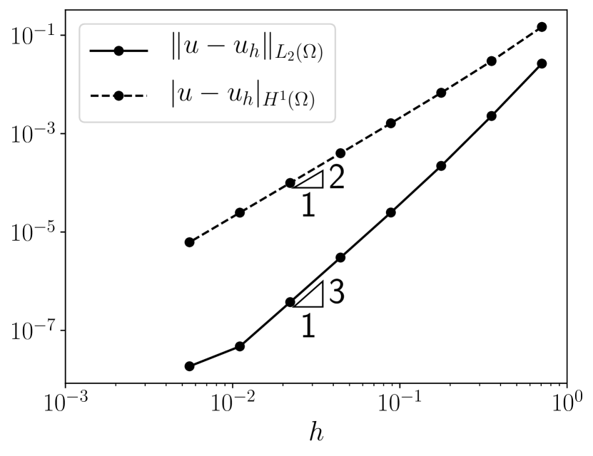
(a)

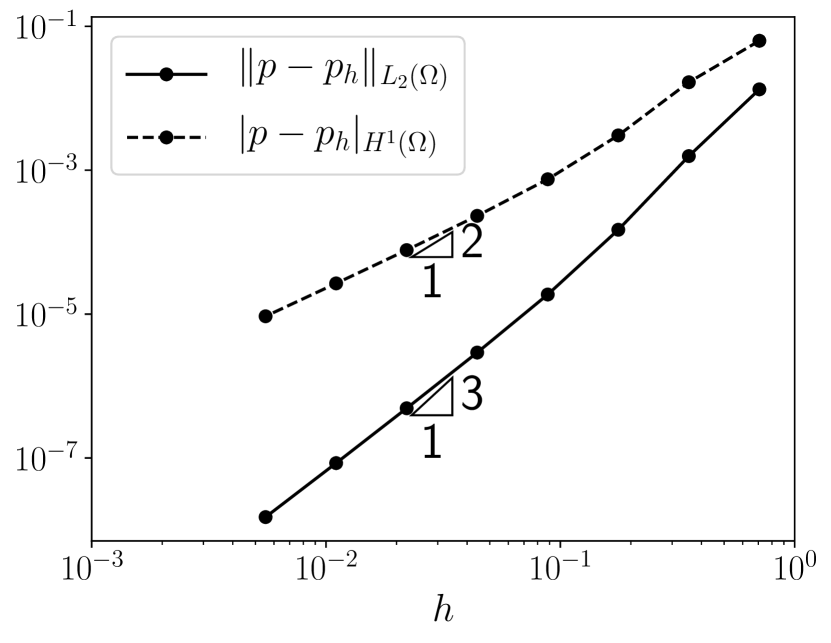
(b)

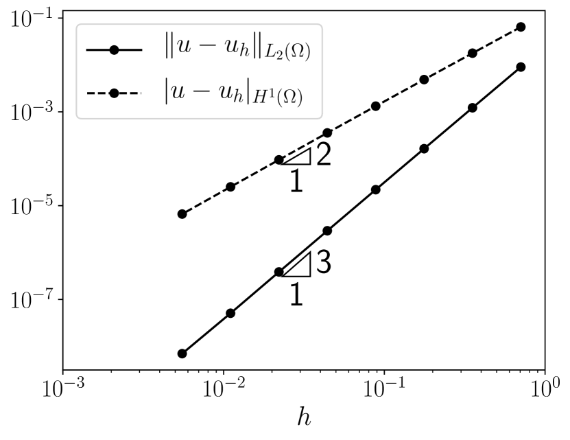
(c)

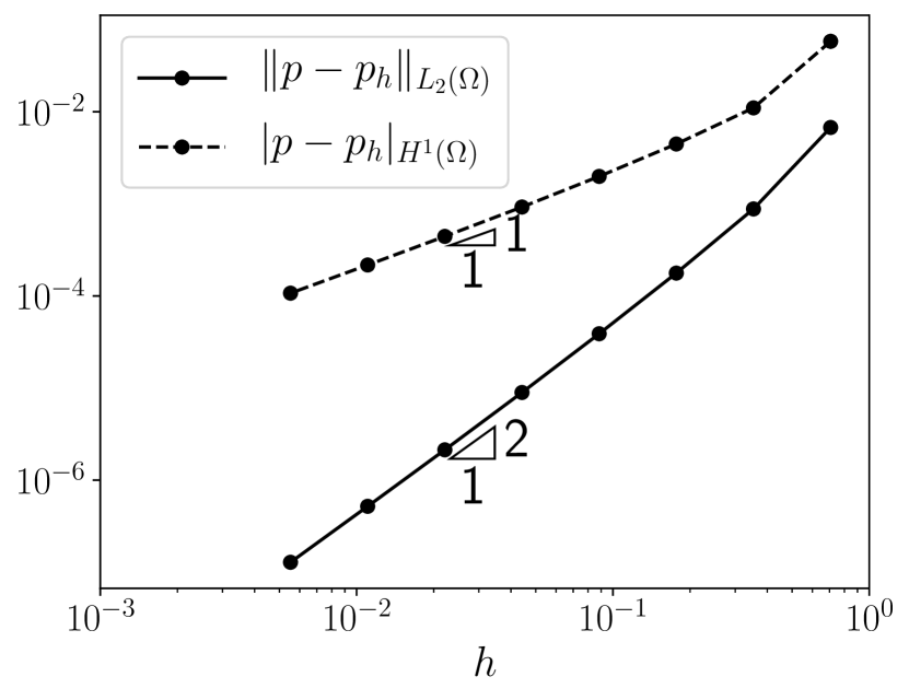
(d)

Figure 3: Example 1: Convergence of the FEM Stokes system with $h$-refinement. Case 1: (a) velocity solution, (b) pressure solution. Case 2: (c) velocity solution, (d) pressure solution.

5.2 Example 2: Manufactured solution - Babuška’s paradox

Babuška’s paradox is a well known problem in computational solid mechanics [7]. It states that with simple support boundary conditions the solution of the Kirchoff-Love plate equation (biharmonic equation) is not the same as the solution of same equations posed on a polygonal domain in the limit approaching the unit disc [7]. This is particularly pertinent in our experiments given that the solution of the Stokes system with free slip boundary conditions may be reformulated in terms of the stream function solution of the biharmonic equation. For more details on Babuška’s paradox in the context of the Stokes system and a review of methods available to alleviate its consequences we refer to [41].

Babuška’s paradox is problematic given that the finite element approximation of the Stokes solution is at the mercy of the variational crime $\Omega\neq\Omega_{h}$. By this we mean that a piecewise polynomial representation of the exterior facets of the mesh may only be an approximation of the disk. In this section we will examine a priori error convergence properties as the computational domain’s fidelity approaches the unit disk. We consider the case where the polynomial representation of the exterior facets is piecewise quadratic.

Here we repeat the manufactured solution numerical experiments of the previous section on the ellipse $\Omega\vcentcolon=\{(x,y)\mathrel{\mathop{\ordinarycolon}}x^{2}+\frac{y^{2}}{(1+\varepsilon_{y})^{2}}<1\}$. Note that the domain is the unit disc in the case that $\varepsilon_{y}=0$. By choosing parameters $\varepsilon_{y}\ll 1$, we can investigate the impact of Babuška’s paradox on the solvability of the problem. The analytical solutions in each case are shown in fig. 2.

The results are shown in fig. 4. In the case that $\varepsilon_{y}=0$, clearly the system does not converge to the true solution, a demonstration of the perplexity of Babuška’s paradox. In the cases that $\varepsilon_{y}>0$ one observes that as the approximation of the ellipse is more precise (i.e. we diverge from the unit disc), the finite element approximation error indicates convergence to the true solution at an optimal rate.

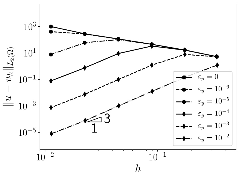
(a)

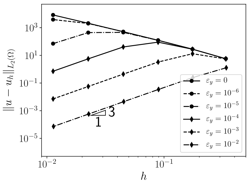
(b)

Figure 4: Example 2: Convergence of the FEM Stokes system in the ellipse with $h$-refinement and free slip boundary conditions. Note that as $\varepsilon_{y}\rightarrow 0$, the finite element velocity solution does not converge to the true velocity solution. (a) Case 1, (b) Case 2.

5.3 Example 3: Steady state isoviscous and nonlinear convection

Case	$\mathrm{Ra}$	$\Delta\eta_{T}$	$\Delta\eta_{z}$	$L$	$\eta$
1	${10}^{4}$	$0$	$0$	1	$\eta_{\text{lin}}$
2	${10}^{5}$	$0$	$0$	1	$\eta_{\text{lin}}$
3	${10}^{6}$	$0$	$0$	1	$\eta_{\text{lin}}$
4	${10}^{4}$	${10}^{3}$	$0$	1	$\eta_{\text{lin}}$
5	${10}^{4}$	$16\,384$	$64$	2.5	$\eta_{\text{lin}}$

(a) Blankenbach [12] benchmark cases.

Case	$\mathrm{Ra}$	$\Delta\eta_{T}$	$\Delta\eta_{z}$	$\eta^{*}$	$\sigma_{Y}$	$L$	$\eta$
1	${10}^{2}$	${10}^{5}$	$1$			1	$\eta_{\text{lin}}$
2	${10}^{2}$	${10}^{5}$	$1$	${10}^{-3}$	$1$	1	$\eta_{\text{total}}$
3	${10}^{2}$	${10}^{5}$	$10$			1	$\eta_{\text{lin}}$
4	${10}^{2}$	${10}^{5}$	$10$	${10}^{-3}$	$1$	1	$\eta_{\text{total}}$

(b) Tosi [40] benchmark cases.

Table 1: Benchmark cases and their corresponding viscosity model parameters.

The first numerical example of a geophysical Boussinesq system is the steady state benchmark problems collated by Blankenbach et al. [12] and additional similar benchmarks collated by Tosi et al. [40]. Here, mantle convection is modelled in a rectangular cell of length $L$ and height $H=1$ such that $\Omega\mathrel{\mathop{\ordinarycolon}}=(0,L)\times(0,H)$. The domain is meshed into $2\times\mathfrak{m}\times\mathfrak{n}$ regular triangle elements where $\mathfrak{m}$ and $\mathfrak{n}$ are the number of bisected squares in the $x$ and $y$ directions, respectively. On these meshes we compute the finite element approximation of the Boussinesq system eqs. 20, 21 and 22. The source term in the Stokes system is given by

$$f=\mathrm{Ra}\>T\hat{k},$$ (26)

where $\mathrm{Ra}$ is the dimensionless Rayleigh number and $\hat{k}=(0,1)^{\top}$ is the unit vector pointing in the direction of buoyancy. The viscosity $\eta$ given in terms of

$$\eta_{\text{lin}} =e^{-\ln(\Delta\eta_{T})T+\ln(\Delta\eta_{z})z}, \eta_{\text{plast}} =\eta^{*}+\frac{\sigma_{Y}}{\sqrt{\varepsilon(u)\mathrel{\mathop{\ordinarycolon}}\varepsilon(u)}}, \eta_{\text{total}} =2\mathinner{\left(\eta_{\text{lin}}^{-1}+\eta_{\text{plast}}^{-1}\right)}^{-1},$$ (27)

where $z=1-y$ is the depth from the lid (located at $z=0$) and $\Delta\eta_{T}$ and $\Delta\eta_{z}$ are constant parameters. $\sigma_{Y}$ is the yield stress, $\eta^{*}\ll 1$ is a constant and $\sqrt{\varepsilon(u)\mathrel{\mathop{\ordinarycolon}}\varepsilon(u)}$ is the second invariant of the rate of strain tensor. The non–dimensional thermal diffusivity $\kappa=1$ and heat source $Q=0$ in all cases.

The boundary conditions require that a free slip boundary condition is applied on $\Gamma_{S}=\partial\Omega$ and that the temperature at the base and top of the cell is prescribed to be $T|_{y=0}=1$ and $T|_{y=H}=0$. Finally $\nabla T\cdot n=0$ on the left $x=0$ and right $x=L$ boundaries.

Five steady state benchmark cases are examined from the work by Blankenbach et al. [12] and four steady state benchmark cases showcased by Tosi et al. [40]. The parameters employed in these benchmarks are shown in table 1, respectively. The key difference between the two benchmarks is the viscosity model. The Blankenbach et al. benchmarks focus on linear, temperature and depth dependent viscosity, whereas the Tosi et al. benchmark includes a visco-plastic model dependent on temperature and rate of strain, giving rise to a nonlinear system of equations.

To find the finite element solution we initially use a fixed point iteration between the Stokes and temperature subsystems. After around $10$ fixed point iterations, the approximation is supplied as an initial guess to a Newton solver for subsequent solution. Convergence is satisfied if the absolute value of the $2-$norm of the finite element residual vector is less than ${10}^{-10}$. See [43] for an example of the fixed point method in this context.

A complete list of computed functionals and their tabulation with mesh refinement are given in appendix A where the free slip boundary conditions are enforced in both the strong and weak sense for comparison. For brevity, here we show the computed top Nusselt number

$$\mathrm{Nu}_{\text{top}}=\frac{\int_{\Gamma_{\text{top}}}\nabla T\cdot n\operatorname{d\!}{s}}{\int_{\Gamma_{\text{bottom}}}T\operatorname{d\!}{s}}$$ (28)

from the benchmark cases solved with weakly imposed free slip boundary conditions in fig. 5 and table 2, respectively. Here $\Gamma_{\text{top}}$ and $\Gamma_{\text{bottom}}$ correspond to the exterior boundaries at $y=H$ and $y=0$, respectively. All functionals converge in agreement with the literature. Furthermore, the results computed from the strong and weak imposition of the boundary conditions compare favourably as shown in appendix A.

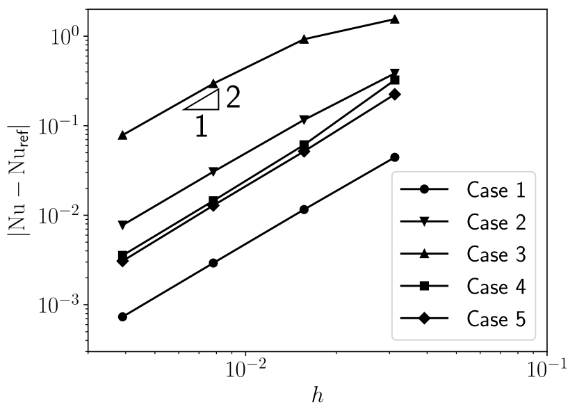
(a)

Figure 5: Example 3: Convergence of the computed top Nusselt number approximation in the Blankenbach et al. [12] benchmark using Nitsche’s method to enforce the free slip boundary condition. See table 1 for a list of parameters. In case 5 of the Blankenbach et al. benchmarks, $\mathfrak{m}=\frac{5}{2}\mathfrak{n}$. The reference values $\mathrm{Nu}_{\text{ref}}$ used are obtained from [43].

Code	$\mathfrak{m}$	Case 1	Case 2	Case 3	Case 4
This work	32	$3.420\,410$	$8.696\,873$	$3.034\,962$	$6.711\,525$
	64	$3.424\,483$	$8.603\,156$	$3.035\,024$	$6.642\,305$
	128	$3.424\,629$	$8.571\,444$	$3.034\,917$	$6.622\,504$
	256	$3.424\,609$	$8.562\,694$	$3.034\,883$	$6.617\,284$
StagYY	128	$3.419$	$8.5491$	$3.030\,25$	$6.610\,82$
Fluidity	128	$3.4253$	$8.5693$	$3.0399$	$6.6401$
ASPECT	64	$3.4305$	$8.5758$	$3.0371$	$6.6249$

Table 2: Example 3: Computed top Nusselt number values $\mathrm{Nu}_{\text{top}}$ using Nitsche’s method to enforce the free slip boundary conditions of the benchmark [40]. Reference values from finite element codes are selected from [40] for comparison. See table 1 for a list of parameters.

5.4 Example 4: Subduction zone

The subduction zone model in this section comprises a downward sloping slab incident to an overriding plate lying below the lithosphere. We will reproduce the numerical benchmark undertaken in [42]. Note however, that in this benchmark the velocity at the interface between the downward sloping slab and the overriding plate is not prescribed in the sense of zero penetration, but rather a fixed velocity boundary. In this section we take a departure from this requirement of the benchmark in favour of a comparison of prescribed velocity data and a free slip (no penetration) boundary condition between the subducting slab and overriding plate using Nitsche’s method. We validate our experiments by reproducing the numerical experiment cases 1c, 2a and 2b undertaken in the benchmark [42].

5.4.1 Geometry

The geometry and boundary conditions of this example problem are exhibited in fig. 6. Specifically, the geometry is composed of a $(0,Z(\tan\alpha)^{-1}+\delta_{x})\times(0,-Z)$ rectangle, where $Z=$600\text{\,}\mathrm{km}$$ is the slab depth, $\alpha=\pi/4$ is the dipping angle of the slab (measured from the top of the overriding lithosphere) and $\delta_{x}=$60\text{\,}\mathrm{km}$$ is a small extension in the $x$ direction. The rectangle is divided by a line whose source lies at $(0,0)$ and terminates at $(Z(\tan\alpha)^{-1},-Z)$. The overriding plate extends from this subduction interface at a constant depth of $Z_{\text{plate}}=$50\text{\,}\mathrm{km}$$ and terminating at $(Z(\tan\alpha)^{-1}+\delta_{x},-Z_{\text{plate}})$.

5.4.2 Boundary conditions

The velocity boundary conditions are as follows: The incoming slab is incident with velocity $u=u_{\text{inlet}}$ on the left side boundary $x=0$, no slip $u=0$ on the overriding plate $y=-Z_{\text{plate}}$ and a prescribed velocity of the subducting slab in the right oriented tangential direction $u=\tau_{r}$ above the the plate depth $y>-Z_{\text{plate}}$ where

$$\tau_{r}=\begin{cases}\tau&\text{if }\tau_{x}>0,\\ -\tau&\text{otherwise}.\end{cases}$$ (29)

Natural boundary conditions are enforced on the remaining exterior boundary. On the remaining slab interface lying below the overriding plate, $\Gamma_{\text{slab}}$, we choose to enforce either a free slip boundary condition $u\cdot n=0$ or prescribed tangential flow $u=\tau_{r}$.

The temperature boundary conditions are as follows: on the top exterior boundary $T(x,0)=T_{\text{s}}$, on the left boundary $T(0,y)=T_{\text{left}}$ and on the right exterior boundary $T(Z(\tan\alpha)^{-1}+\delta_{x},y)=T_{\text{right}}$, where the quantities

$$T_{\text{s}} =$273$,$$

$$T_{\text{left}} =T_{\text{s}}+\mathinner{\left(T_{0}-T_{\text{s}}\right)}\mathrm{erf}\mathinner{\left(-y\frac{${10}^{3}$}{2\sqrt{\kappa t_{$50$}}}\right)},$$

$$T_{\text{right}} =\begin{cases}T_{\text{s}}-$0.026\text{\times}{10}^{3}$y&\text{if }y>-Z_{\text{plate}},\\ T_{0}&\text{otherwise}.\end{cases}$$ (30)

Here $T_{0}=$1573\text{\,}\mathrm{K}$$ is the inlet temperature, $t_{$50$}=$50\text{\times}{10}^{6}$\times$365$\times$24$\times$60$^{2}$ is the age of the $50\text{\,}\mathrm{Myr}$ old plate in seconds and the thermal diffusivity $\kappa=$0.7272\text{\times}{10}^{-6}\text{\,}{\mathrm{m}}^{2}\text{\,}{\mathrm{s}}^{-1}$$.

5.4.3 Viscosity and slab surface models

We consider the following cases which are named corresponding with the work [42]:

1. The linear isoviscous case $\eta=1$.

2. A nonlinear diffusion creep model with viscosity

   $$\eta_{\text{diff}}=A_{\text{diff}}\exp\mathinner{\left(\frac{E_{\text{diff}}}{RT}\right)},$$ (31)

   where $A_{\text{diff}}=$1.320\,43\text{\times}{10}^{9}$$, $E_{\text{diff}}=$335\text{\times}{10}^{3}$$ and $R=$8.3145$$ from which the total viscosity

   $$\eta=\left(\eta_{\text{max}}^{-1}+\eta_{\text{diff}}^{-1}\right)^{-1},$$ (32)

   where $\eta_{\text{max}}=${10}^{26}$$.

3. A nonlinear dislocation creep model with viscosity

   $$\eta_{\text{disl}}=A_{\text{disl}}\exp\left(\frac{E_{\text{disl}}}{n_{\text{exp}}RT}\right)\varepsilon_{\mathrm{II}}^{\frac{1-n_{\text{exp}}}{n_{\text{exp}}}},$$ (33)

   where $A_{\text{disl}}=$29\,868.6$$, $E_{\text{disl}}=$540\text{\times}{10}^{3}$$, $n_{\text{exp}}=$3.5$$ and $\varepsilon_{\mathrm{II}}=\sqrt{\frac{1}{2}\varepsilon(u)\mathrel{\mathop{\ordinarycolon}}\varepsilon(u)}$, from which the total viscosity is given by

   $$\eta=\left(\eta_{\text{max}}^{-1}+\eta_{\text{disl}}^{-1}\right)^{-1}.$$ (34)

As an extension of [42] we consider cases 1c and 2b with a curved slab geometry. This curve is described by the parabola

$$y_{\text{slab}}=-Z\left(\frac{x}{Z}\right)^{n_{\text{slab}}},$$ (35)

where $n_{\text{slab}}=$2.5$$. The inlet velocity is prescribed separately for the two slab geometry schemes. In the case of the straight subducting slab $u_{\text{inlet}}=(\cos(\alpha),-\sin(\alpha))^{\top}$. And in the case of the curved slab $u_{\text{inlet}}=-n$.

5.4.4 Solution technique

Note that the nonlinearity in this problem is numerically challenging to resolve. We first employ a fixed point iterative method to obtain an initial guess for subsequent solution by Newton’s iterative method. Additionally, we must resolve the pressure discontinuity across the subducting slab. Although it is suboptimal, we choose the $W^{h,0}$ velocity–pressure–temperature finite element space where $\mathfrak{s}=1$ as defined in section 3, i.e. piecewise constant pressure approximation.

5.4.5 Results

The temperature field from these computations is shown in fig. 7. In the straight subducting slab computation where $u=\tau_{r}$ on $\Gamma_{\text{slab}}$ the following functionals are computed for validation and comparison with the community benchmark:

$$T_{11,11} =T(\xi_{11,11})-T_{s},$$ (36)

$$\|T_{\text{slab}}\| =\sqrt{\frac{\sum_{i=1}^{36}\mathinner{\left(T(\xi_{ii})-T_{s}\right)}^{2}}{36}},$$ (37)

$$\|T_{\text{wedge}}\| =\sqrt{\frac{\sum_{i=10}^{21}\sum_{j=10}^{i}\mathinner{\left(T(\xi_{ij})-T_{s}\right)}^{2}}{78}},$$ (38)

where $\xi_{ij}=(6(i-1),-6(j-1))^{\top}$ forms a series of discrete equidistant points with interval spacing of $6$ originating at $(0,0)$, see [42] for details. The computed functionals are tabulated in table 3.

Case	Code	$T_{11,11}$	$\|T_{\text{slab}}\|$	$\|T_{\text{wedge}}\|$
1c	This work	$387.86$	$503.18$	$853.04$
	Reference	$387.84$	$503.13$	$852.92$
2a	This work	$579.43$	$606.50$	$1002.52$
	Reference	$580.66$	$607.11$	$1003.20$
2b	This work	$582.01$	$604.46$	$999.12$
	Reference	$583.36$	$605.11$	$1000.01$

Table 3: Example 4: Computed benchmark functionals for comparison with [42] where the reference data is quoted from the UM contributing finite element code. The temperature fields computed in these problems are shown in fig. 7. The minimum and maximum cell circumradii used in the mesh are $0.161$ and $24.9$, respectively.

Case	$\Gamma_{\text{slab}}$ condition	$T_{11,11}$	$\|T_{\text{slab}}\|$	$\|T_{\text{wedge}}\|$	$T(x_{\text{slab}},-60)$
1c	$u=\tau_{r}$	$991.12$	$1093.15$	$1055.66$	$352.80$
	$u\cdot n=0$	$982.49$	$1066.46$	$1028.21$	$171.339$
2b	$u=\tau_{r}$	$961.74$	$1071.79$	$1026.13$	$557.84$
	$u\cdot n=0$	$961.74$	$1071.73$	$1021.58$	$614.83$

Table 4: Example 4: Computed benchmark functionals in the curved subducting slab case. Here $n_{\text{slab}}=$2.5$$. The temperature fields computed in these problems are shown in fig. 7. The minimum and maximum cell circumradii used in the mesh are $0.134$ and $24.1$, respectively.

Examine the two cases where $u=\tau_{r}$ on $\Gamma_{\text{slab}}$ and the slab geometry is curved in fig. 7. These cases are the extension of cases 1c and 2b exhibited in [42]. We introduce one more functional for with the curved geometry experiments, $T(x_{\text{slab}},-60)$. This is the analogy of $T_{11,11}$ for the curved geometry, i.e., the temperature measured on the slab–wedge boundary at a depth of $y_{\text{slab}}=$60$$ where

$$x_{\text{slab}}=Z\sqrt[n_{\text{slab}}]{\frac{-y_{\text{slab}}}{Z}}.$$ (39)

The computed functionals from these experiments are shown in table 4.

The plots of the temperature fields from the final two cases where $u\cdot n=0$ on $\Gamma_{\text{slab}}$ and the slab geometry is curved invites curiosity. There is an apparent change in the mantle flow profile at the plate depth compared with the previous cases. These changes are primarily due to the benchmark [42] requiring the overlap of the discontinuity $u=0$ on the plate boundary and $u=\tau_{r}$ on the upper subducting slab. The lower subducting slab on $\Gamma_{\text{slab}}$ and boundary condition $u\cdot n=0$ propagates the single node data on which $u=0$ is enforced. This results in the velocity ‘bump’ observed. Examination of the velocity streamlines elucidates this as shown in fig. 8. The work [42] discusses the issue of this boundary condition overlap in greater detail. If we were to enforce the free slip boundary condition strongly, indeed we may isolate the single degree of freedom associated with the overriding plate and subducting slab node and enforce a free slip condition. Nitsche’s method is mathematically consistent and does not permit such ‘variational crimes’.

Figure 6: The $(0,Z(\tan\alpha)^{-1}+\delta_{x})\times(0,-Z)$ rectangle subduction zone problem geometry. The subduction slab is defined by a line sourced at $(0,0)$ and terminating at $(Z(\tan\alpha)^{-1},-Z)$.

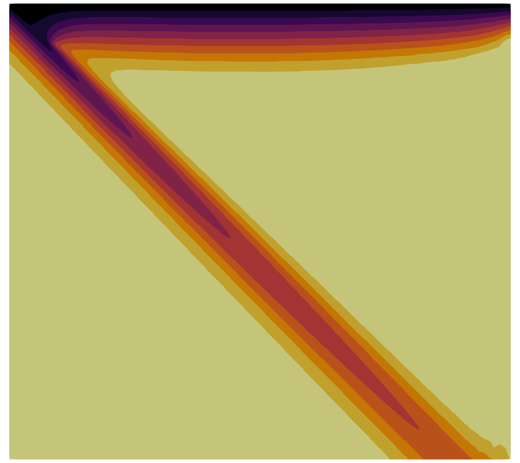
(a) Case 1c, $u=\tau_{r}$ on $\Gamma_{\text{slab}}$

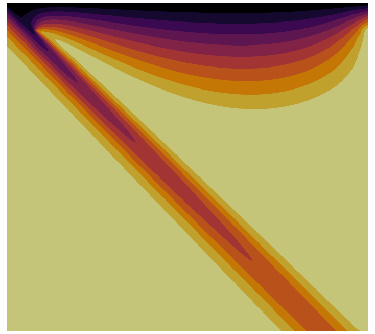
(b) Case 2b, $u=\tau_{r}$ on $\Gamma_{\text{slab}}$

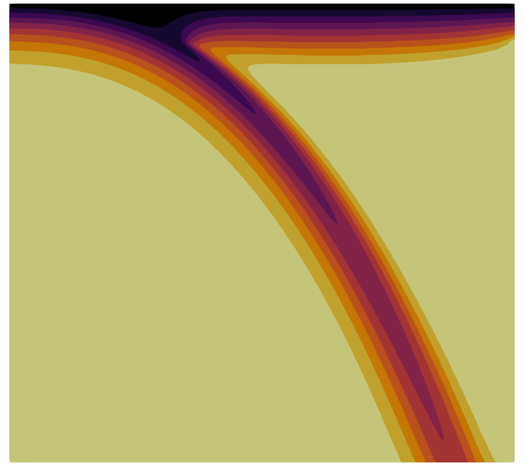
(c) Case 1c, $u=\tau_{r}$ on $\Gamma_{\text{slab}}$

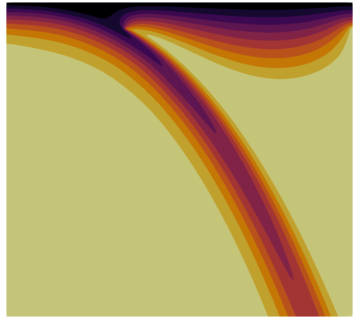
(d) Case 2b, $u=\tau_{r}$ on $\Gamma_{\text{slab}}$

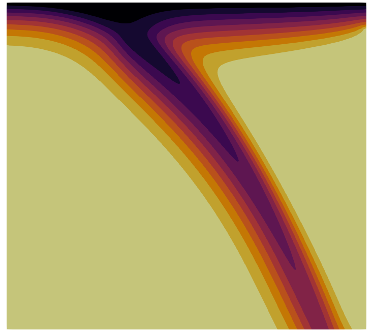
(e) Case 1c, $u\cdot n=0$ on $\Gamma_{\text{slab}}$

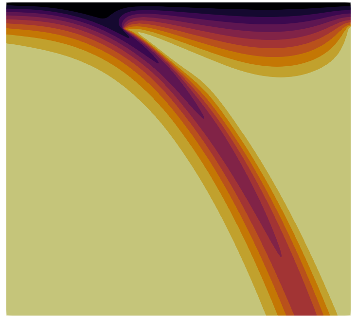
(f) Case 2b, $u\cdot n=0$ on $\Gamma_{\text{slab}}$

Figure 7: Example 4: Subduction zone with: (a) & (b) straight subducting slab where $\alpha=\frac{\pi}{4}$; (c), (d), (e) & (f) curved subducting slab defined by eq. 35 where $n_{\text{slab}}=2.5$. The geometry and model are described in section 5.4.

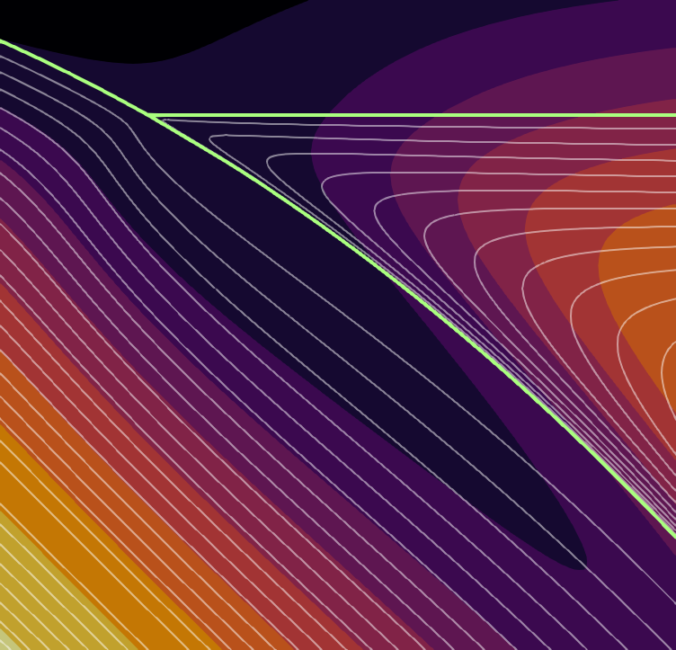
(a) Case 1c, $u\cdot n=0$ on $\Gamma_{\text{slab}}$

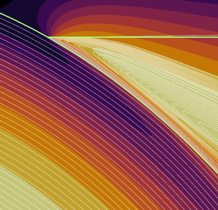
(b) Case 2b, $u\cdot n=0$ on $\Gamma_{\text{slab}}$

Figure 8: Example 4: Examination of the streamlines in Cases 1c and 2b where $u\cdot n=0$ on $\Gamma_{\text{slab}}$. The geometry of the subduction interface and overriding plate is overlaid in green. The temperature fields in the whole geometry are shown in fig. 7. (a) shows the overlap of the no–slip boundary condition on the overriding plate manifests prominently. (b) shows that the dislocation creep viscosity model is less affected by this numerical artifact. The nature of this boundary condition is discussed in detail in [42]. Here, the streamlines in both (a) and (b) are generated from $200$ equidistant source points located on the left ($x=0$) and right ($x=Z(\tan\alpha)^{-1})+\delta_{x}$) boundary.

5.5 Example 5: Iterative solvers and 3D geometry

In this final example we demonstrate the viability of Nitsche’s method with Krylov subspace iterative solvers. Rigorous demonstration of scalable solvers for finite element problems in computational geodynamics is available in [31]. In this work we are concerned with the conditioning of the underlying finite element matrix, subject to the penalty parameter in Nitsche’s method, $C_{\text{IP}}\ell^{2}/h_{F}$ (see sections 2.3 and 2.4). With the experiments exhibited in this section we seek to alleviate the worry that including a penalty parameter in the finite element formulation will cause preconditioned Krylov subspace solvers to fail to converge.

Motivated by the results in the previous section, we consider the case 1c, where $u\cdot n=0$ on $\Gamma_{\text{slab}}$. We further choose the curved subducting slab geometry where $n_{\text{slab}}=1.5$. Our numerical experiment in this section will compute the finite element approximation on a hierarchical sequence of meshes. The first mesh is a coarse representation of the geometry, and the sequence defines progressively finer meshes which are adaptively generated based on residual–based error estimation of the finite element solution. Other examples of adaptive refinement using the tools showcased in this work are demonstrated in [25].

We will solve the problem in a 2D and 3D geometry. The 2D geometry is as described in the previous section. To generate the 3D geometry we extrude the 2D geometry by rotating $\frac{\pi}{4}$ radians about the $(0,1,0)$ axis centred at $(-Z_{\text{plate}},0,0)$. On the new near and far side faces we apply the free slip boundary condition. All other boundary conditions are the extrusion of the 2D case.

Newton’s iterative method is used to solve the finite element system. We solve the underlying linear system using an outer fGMRES solver with an inverse viscosity pressure mass matrix preconditioner for the pressure block, cf. [31]. We construct the linear solver as follows: for the velocity block we apply a GMRES smoother with PETSc’s geometric algebraic multigrid preconditioner with smoothed aggregation; on the pressure block a conjugate gradient smoother with HYPRE-BoomerAMG preconditioner; on the temperature block we use a GMRES smoother with HYPRE-BoomerAMG preconditioner.

In each experiment we measure the total number of degrees of freedom (DoF), the maximum and minimum mesh cell dihedral angles $h_{\text{max}}$ and $h_{\text{min}}$, respectively, the number of fGMRES iterations $n_{\text{Krylov}}$, the number of Newton iterations $n_{\text{Newton}}$ and the final finite element vector residual in the 2–norm $\|r\|_{2}$. The tabulated results of the two experiments are shown in table 5. The computed finite element temperature field in the 3D geometry is shown in fig. 9.

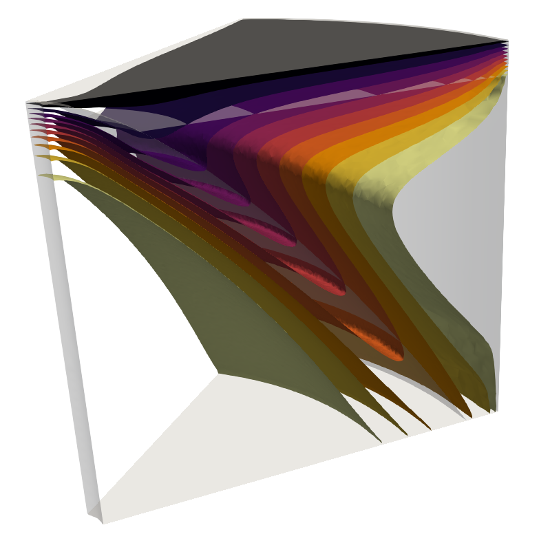
Figure 9: Example 5: Temperature field isosurfaces from the 3D computation overlaying the semitransparent extruded geometry described in section 5.5. Here $n_{\text{slab}}=1.5$.

	DoF	$h_{\text{max}}$	$h_{\text{min}}$	$n_{\text{Krylov}}$	$n_{\text{Newton}}$	$\|r\|_{2}$
2D	$14\,956$	$28.6$	$13.5$	$45$	$4$	$7.7545\text{\times}{10}^{-09}$
	$34\,136$	$25.4$	$6.51$	$45$	$4$	$8.2716\text{\times}{10}^{-09}$
	$77\,226$	$25.7$	$3.45$	$47$	$4$	$9.2493\text{\times}{10}^{-09}$
	$168\,552$	$25.5$	$1.82$	$45$	$4$	$5.0943\text{\times}{10}^{-09}$
	$358\,146$	$25.2$	$0.889$	$44$	$4$	$7.6659\text{\times}{10}^{-09}$
	$747\,281$	$25.9$	$0.481$	$43$	$4$	$7.5715\text{\times}{10}^{-09}$
	$1\,542\,503$	$24.0$	$0.220$	$43$	$4$	$4.7911\text{\times}{10}^{-09}$
	$3\,156\,039$	$25.2$	$0.111$	$42$	$4$	$9.6823\text{\times}{10}^{-09}$
	$6\,338\,077$	$68.0$	$0.0342$	$42$	$4$	$5.9607\text{\times}{10}^{-09}$
	$14\,248\,941$	$46.9$	$0.0227$	$39$	$4$	$8.0802\text{\times}{10}^{-09}$
	$20\,979\,279$	$46.7$	$0.0114$	$56$	$5$	$4.9678\text{\times}{10}^{-09}$
3D	$324\,556$	$50.7$	$16.2$	$154$	$5$	$6.5248\text{\times}{10}^{-09}$
	$1\,012\,848$	$46.1$	$8.71$	$108$	$5$	$8.5585\text{\times}{10}^{-09}$
	$3\,656\,383$	$45.1$	$4.10$	$176$	$5$	$9.4709\text{\times}{10}^{-09}$
	$5\,495\,723$	$42.6$	$3.11$	$156$	$5$	$9.3598\text{\times}{10}^{-09}$

Table 5: Example 5: Examination of the viability of free slip boundary conditions enforced via Nitsche’s method when using a Krylov subspace iterative solver. Viability is indicated by a near–constant number of Krylov subspace iterations required to find convergence of the finite element residual. Here, we consider satisfactory convergence when $\|r\|_{2}<${10}^{-8}$.$

6 Conclusion

The formulation and examples presented in this work elucidate the use of Nitsche’s method for complex problems in geodynamics which require free slip boundary conditions. Additionally we have presented a flexible computational implementation which requires only a symbolic representation of the numerical flux function $\mathcal{F}^{v}(\cdot,\cdot)$ to automatically formulate Nitsche boundary conditions. The author emphasises that we are not limited to the Stokes equations nor free slip boundary conditions with the developed computational tools.

Acknowledgements

The authors wish to thank P. E. van Keken of the Carnegie Institution for Science, Department of Terrestrial Magnetism for his advice, particularly regarding section 5.4. NS gratefully acknowledges the support of Carnegie Institution for Science President’s Fellowship.

Appendix A Blankenbach et al. and Tosi et al. benchmark results

In this section we tabulate the results computed from a reproduction of the Blankenbach et al. [12] and Tosi et al. [40] benchmarks. This data is shown in tables 7 and 8, respectively. The functionals of interest computed from the benchmark FEM solutions are shown in table 6.

Blankenbach et al. [12]
Nusselt number	$\mathrm{Nu}=\frac{\int_{\Gamma_{\text{top}}}\nabla T\cdot n\operatorname{d\!}{s}}{\int_{\Gamma_{\text{bottom}}}T\operatorname{d\!}{s}}$
Heat flux	$\xi_{i}=\left.\left(\nabla T\cdot n\right)\right|_{x=x_{i}}$
	$x_{1}=(0,0),x_{2}=(L,0),$
	$x_{3}=(0,H),x_{4}=(L,H)$
Tosi et al. [40]
Top Nusselt number	$\mathrm{Nu}_{\text{top}}=\frac{\int_{\Gamma_{\text{top}}}\nabla T\cdot n\operatorname{d\!}{s}}{\int_{\Gamma_{\text{bottom}}}T\operatorname{d\!}{s}}$
Bottom Nusselt number	$\mathrm{Nu}_{\text{bottom}}=\frac{\int_{\Gamma_{\text{bottom}}}\nabla T\cdot n\operatorname{d\!}{s}}{\int_{\Gamma_{\text{top}}}T\operatorname{d\!}{s}}$
Average temperature	$\langle T\rangle=\frac{\int_{\Omega}T\operatorname{d\!}{x}}{\int_{\Omega}\operatorname{d\!}{x}}$
Root-mean-square (RMS) velocity	$u_{\text{rms}}=\sqrt{\frac{\int_{\Omega}u\cdot u\operatorname{d\!}{x}}{\int_{\Omega}\operatorname{d\!}{x}}}$
Surface RMS velocity	$u_{\text{surf rms}}=\sqrt{\frac{\int_{\Gamma_{\text{top}}}u\cdot u\operatorname{d\!}{s}}{\int_{\Gamma_{\text{top}}}\operatorname{d\!}{s}}}$
Average rate of viscous dissipation	$\langle\Phi\rangle=\frac{\int_{\Omega}2\eta\varepsilon(u)\mathrel{\mathop{\ordinarycolon}}\varepsilon(u)\operatorname{d\!}{x}}{\int_{\Omega}\operatorname{d\!}{x}}$
Average work done against gravity	$\langle W\rangle=\frac{\int_{\Omega}Tu_{y}\operatorname{d\!}{x}}{\int_{\Omega}\operatorname{d\!}{x}}$

Table 6: The functionals computed in the Blankenbach et al. and Tosi et al. benchmarks. Here $\Gamma_{\text{top}}$ and $\Gamma_{\text{bottom}}$ correspond to the exterior boundaries at $y=H$ and $y=0$, respectively.

$\mathfrak{m}$	$\mathfrak{n}$	$\mathrm{Nu}$		$\xi_{1}$		$\xi_{2}$		$\xi_{3}$		$\xi_{4}$
$32$	$32$	$4$	$.92878$	$0$	$.56810$	$8$	$.21398$	$8$	$.21398$	$0$	$.56810$
$64$	$64$	$4$	$.89600$	$0$	$.58353$	$8$	$.09761$	$8$	$.09761$	$0$	$.58353$
$128$	$128$	$4$	$.88734$	$0$	$.58748$	$8$	$.06891$	$8$	$.06891$	$0$	$.58748$
$256$	$256$	$4$	$.88514$	$0$	$.58848$	$8$	$.06177$	$8$	$.06177$	$0$	$.58848$

(a) Case 1: strong

$\mathfrak{m}$	$\mathfrak{n}$	$\mathrm{Nu}$		$\xi_{1}$		$\xi_{2}$		$\xi_{3}$		$\xi_{4}$
$32$	$32$	$4$	$.92881$	$0$	$.56810$	$8$	$.21400$	$8$	$.21400$	$0$	$.56810$
$64$	$64$	$4$	$.89600$	$0$	$.58353$	$8$	$.09761$	$8$	$.09761$	$0$	$.58353$
$128$	$128$	$4$	$.88734$	$0$	$.58748$	$8$	$.06891$	$8$	$.06891$	$0$	$.58748$
$256$	$256$	$4$	$.88514$	$0$	$.58848$	$8$	$.06177$	$8$	$.06177$	$0$	$.58848$

(b) Case 1: weak

$\mathfrak{m}$	$\mathfrak{n}$	$\mathrm{Nu}$		$\xi_{1}$		$\xi_{2}$		$\xi_{3}$		$\xi_{4}$
$32$	$32$	$10$	$.91892$	$0$	$.57517$	$21$	$.08205$	$21$	$.08205$	$0$	$.57517$
$64$	$64$	$10$	$.65041$	$0$	$.68205$	$19$	$.62050$	$19$	$.62050$	$0$	$.68205$
$128$	$128$	$10$	$.56473$	$0$	$.71244$	$19$	$.21224$	$19$	$.21224$	$0$	$.71244$
$256$	$256$	$10$	$.54185$	$0$	$.72017$	$19$	$.11246$	$19$	$.11246$	$0$	$.72017$

(c) Case 2: strong

$\mathfrak{m}$	$\mathfrak{n}$	$\mathrm{Nu}$		$\xi_{1}$		$\xi_{2}$		$\xi_{3}$		$\xi_{4}$
$32$	$32$	$10$	$.91955$	$0$	$.57521$	$21$	$.08243$	$21$	$.08243$	$0$	$.57521$
$64$	$64$	$10$	$.65047$	$0$	$.68205$	$19$	$.62058$	$19$	$.62058$	$0$	$.68205$
$128$	$128$	$10$	$.56473$	$0$	$.71244$	$19$	$.21225$	$19$	$.21225$	$0$	$.71244$
$256$	$256$	$10$	$.54186$	$0$	$.72017$	$19$	$.11246$	$19$	$.11246$	$0$	$.72017$

(d) Case 2: weak

$\mathfrak{m}$	$\mathfrak{n}$	$\mathrm{Nu}$		$\xi_{1}$		$\xi_{2}$		$\xi_{3}$		$\xi_{4}$
$32$	$32$	$23$	$.52241$	$0$	$.42235$	$45$	$.70460$	$45$	$.70460$	$0$	$.42235$
$64$	$64$	$22$	$.89737$	$0$	$.62169$	$52$	$.09406$	$52$	$.09406$	$0$	$.62169$
$128$	$128$	$22$	$.26786$	$0$	$.80242$	$47$	$.93502$	$47$	$.93502$	$0$	$.80242$
$256$	$256$	$22$	$.05103$	$0$	$.85821$	$46$	$.44536$	$46$	$.44536$	$0$	$.85821$

(e) Case 3: strong

$\mathfrak{m}$	$\mathfrak{n}$	$\mathrm{Nu}$		$\xi_{1}$		$\xi_{2}$		$\xi_{3}$		$\xi_{4}$
$32$	$32$	$23$	$.52555$	$0$	$.42298$	$45$	$.68845$	$45$	$.68845$	$0$	$.42298$
$64$	$64$	$22$	$.89885$	$0$	$.62174$	$52$	$.09446$	$52$	$.09446$	$0$	$.62174$
$128$	$128$	$22$	$.26802$	$0$	$.80242$	$47$	$.93529$	$47$	$.93529$	$0$	$.80242$
$256$	$256$	$22$	$.05105$	$0$	$.85821$	$46$	$.44538$	$46$	$.44538$	$0$	$.85821$

(f) Case 3: weak

$\mathfrak{m}$	$\mathfrak{n}$	$\mathrm{Nu}$		$\xi_{1}$		$\xi_{2}$		$\xi_{3}$		$\xi_{4}$
$32$	$32$	$10$	$.39876$	$0$	$.25302$	$26$	$.23297$	$19$	$.35305$	$0$	$.89641$
$64$	$64$	$10$	$.12751$	$0$	$.33360$	$30$	$.43423$	$17$	$.81654$	$0$	$.98413$
$128$	$128$	$10$	$.08050$	$0$	$.44936$	$28$	$.14022$	$17$	$.59238$	$1$	$.00264$
$256$	$256$	$10$	$.06955$	$0$	$.48536$	$27$	$.13950$	$17$	$.54615$	$1$	$.00705$

(g) Case 4: strong

$\mathfrak{m}$	$\mathfrak{n}$	$\mathrm{Nu}$		$\xi_{1}$		$\xi_{2}$		$\xi_{3}$		$\xi_{4}$
$32$	$32$	$10$	$.39024$	$0$	$.25536$	$26$	$.27840$	$19$	$.33442$	$0$	$.89574$
$64$	$64$	$10$	$.12719$	$0$	$.33380$	$30$	$.45146$	$17$	$.81636$	$0$	$.98404$
$128$	$128$	$10$	$.08051$	$0$	$.44937$	$28$	$.14438$	$17$	$.59247$	$1$	$.00264$
$256$	$256$	$10$	$.06956$	$0$	$.48536$	$27$	$.13982$	$17$	$.54616$	$1$	$.00705$

(h) Case 4: weak

$\mathfrak{m}$	$\mathfrak{n}$	$\mathrm{Nu}$		$\xi_{1}$		$\xi_{2}$		$\xi_{3}$		$\xi_{4}$
$80$	$32$	$7$	$.15695$	$14$	$.49558$	$0$	$.47788$	$0$	$.15877$	$22$	$.72316$
$160$	$64$	$6$	$.98167$	$14$	$.36231$	$0$	$.58387$	$0$	$.17414$	$19$	$.15460$
$320$	$128$	$6$	$.94275$	$14$	$.23152$	$0$	$.60953$	$0$	$.17683$	$18$	$.59655$
$640$	$256$	$6$	$.93298$	$14$	$.18487$	$0$	$.61569$	$0$	$.17728$	$18$	$.50992$

(i) Case 5: strong

$\mathfrak{m}$	$\mathfrak{n}$	$\mathrm{Nu}$		$\xi_{1}$		$\xi_{2}$		$\xi_{3}$		$\xi_{4}$
$80$	$32$	$7$	$.15433$	$14$	$.50981$	$0$	$.47859$	$0$	$.15862$	$22$	$.72285$
$160$	$64$	$6$	$.98164$	$14$	$.36485$	$0$	$.58390$	$0$	$.17413$	$19$	$.15474$
$320$	$128$	$6$	$.94276$	$14$	$.23167$	$0$	$.60954$	$0$	$.17683$	$18$	$.59696$
$640$	$256$	$6$	$.93298$	$14$	$.18487$	$0$	$.61569$	$0$	$.17728$	$18$	$.50996$

(j) Case 5: weak

Table 7: Blankenbach et al. benchmark results. We provide a comparison between strong and weak imposition of the free slip boundary condition. The functionals computed in this experiment match well with the work of Blankenbach et al. [12]

$\mathfrak{m}$	$\mathfrak{n}$	$\mathrm{Nu}_{\text{bottom}}$		$\mathrm{Nu}_{\text{top}}$		$\langle T\rangle$		$u_{\text{rms}}$		$u_{\text{surf rms}}$		$\langle\Phi\rangle$		$\langle W\rangle$
$32$	$32$	$3$	$.64117$	$3$	$.42097$	$0$	$.77564$	$249$	$.23121$	$1$	$.87080$	$242$	$.60976$	$2$	$.42610$
$64$	$64$	$3$	$.52229$	$3$	$.42452$	$0$	$.77603$	$249$	$.76493$	$1$	$.86948$	$242$	$.46196$	$2$	$.42462$
$128$	$128$	$3$	$.45426$	$3$	$.42463$	$0$	$.77605$	$249$	$.80312$	$1$	$.86943$	$242$	$.45966$	$2$	$.42460$
$256$	$256$	$3$	$.43247$	$3$	$.42461$	$0$	$.77605$	$249$	$.80516$	$1$	$.86943$	$242$	$.45982$	$2$	$.42460$

(a) Case 1: strong

$\mathfrak{m}$	$\mathfrak{n}$	$\mathrm{Nu}_{\text{bottom}}$		$\mathrm{Nu}_{\text{top}}$		$\langle T\rangle$		$u_{\text{rms}}$		$u_{\text{surf rms}}$		$\langle\Phi\rangle$		$\langle W\rangle$
$32$	$32$	$3$	$.64612$	$3$	$.42041$	$0$	$.77556$	$249$	$.10828$	$1$	$.87086$	$242$	$.55649$	$2$	$.42585$
$64$	$64$	$3$	$.52332$	$3$	$.42448$	$0$	$.77602$	$249$	$.75746$	$1$	$.86948$	$242$	$.45616$	$2$	$.42461$
$128$	$128$	$3$	$.45435$	$3$	$.42463$	$0$	$.77605$	$249$	$.80285$	$1$	$.86943$	$242$	$.45893$	$2$	$.42460$
$256$	$256$	$3$	$.43248$	$3$	$.42461$	$0$	$.77605$	$249$	$.80515$	$1$	$.86943$	$242$	$.45973$	$2$	$.42460$

(b) Case 1: weak

$\mathfrak{m}$	$\mathfrak{n}$	$\mathrm{Nu}_{\text{bottom}}$		$\mathrm{Nu}_{\text{top}}$		$\langle T\rangle$		$u_{\text{rms}}$		$u_{\text{surf rms}}$		$\langle\Phi\rangle$		$\langle W\rangle$
$32$	$32$	$8$	$.84938$	$8$	$.70626$	$0$	$.60299$	$140$	$.38831$	$104$	$.51937$	$754$	$.64194$	$7$	$.54642$
$64$	$64$	$8$	$.65439$	$8$	$.60258$	$0$	$.60353$	$140$	$.69853$	$104$	$.65930$	$755$	$.68647$	$7$	$.55686$
$128$	$128$	$8$	$.58639$	$8$	$.57102$	$0$	$.60365$	$140$	$.76942$	$104$	$.68760$	$755$	$.92412$	$7$	$.55924$
$256$	$256$	$8$	$.56657$	$8$	$.56249$	$0$	$.60366$	$140$	$.77777$	$104$	$.69095$	$755$	$.95219$	$7$	$.55952$

(c) Case 2: strong

$\mathfrak{m}$	$\mathfrak{n}$	$\mathrm{Nu}_{\text{bottom}}$		$\mathrm{Nu}_{\text{top}}$		$\langle T\rangle$		$u_{\text{rms}}$		$u_{\text{surf rms}}$		$\langle\Phi\rangle$		$\langle W\rangle$
$32$	$32$	$8$	$.90499$	$8$	$.69687$	$0$	$.60224$	$140$	$.06040$	$104$	$.45921$	$754$	$.38337$	$7$	$.53927$
$64$	$64$	$8$	$.65918$	$8$	$.60316$	$0$	$.60344$	$140$	$.68241$	$104$	$.68915$	$756$	$.09145$	$7$	$.55731$
$128$	$128$	$8$	$.58703$	$8$	$.57144$	$0$	$.60361$	$140$	$.76676$	$104$	$.70491$	$756$	$.14260$	$7$	$.55962$
$256$	$256$	$8$	$.56678$	$8$	$.56269$	$0$	$.60364$	$140$	$.77661$	$104$	$.69966$	$756$	$.06151$	$7$	$.55972$

(d) Case 2: weak

$\mathfrak{m}$	$\mathfrak{n}$	$\mathrm{Nu}_{\text{bottom}}$		$\mathrm{Nu}_{\text{top}}$		$\langle T\rangle$		$u_{\text{rms}}$		$u_{\text{surf rms}}$		$\langle\Phi\rangle$		$\langle W\rangle$
$32$	$32$	$3$	$.12933$	$3$	$.03503$	$0$	$.72743$	$100$	$.10242$	$2$	$.07402$	$203$	$.49491$	$2$	$.03495$
$64$	$64$	$3$	$.06307$	$3$	$.03503$	$0$	$.72750$	$100$	$.14310$	$2$	$.07271$	$203$	$.48657$	$2$	$.03487$
$128$	$128$	$3$	$.04234$	$3$	$.03492$	$0$	$.72750$	$100$	$.14587$	$2$	$.07266$	$203$	$.48701$	$2$	$.03487$
$256$	$256$	$3$	$.03677$	$3$	$.03488$	$0$	$.72750$	$100$	$.14605$	$2$	$.07265$	$203$	$.48707$	$2$	$.03487$

(e) Case 3: strong

$\mathfrak{m}$	$\mathfrak{n}$	$\mathrm{Nu}_{\text{bottom}}$		$\mathrm{Nu}_{\text{top}}$		$\langle T\rangle$		$u_{\text{rms}}$		$u_{\text{surf rms}}$		$\langle\Phi\rangle$		$\langle W\rangle$
$32$	$32$	$3$	$.13091$	$3$	$.03496$	$0$	$.72741$	$100$	$.09527$	$2$	$.07408$	$203$	$.49976$	$2$	$.03494$
$64$	$64$	$3$	$.06319$	$3$	$.03502$	$0$	$.72750$	$100$	$.14284$	$2$	$.07271$	$203$	$.48805$	$2$	$.03487$
$128$	$128$	$3$	$.04235$	$3$	$.03492$	$0$	$.72750$	$100$	$.14586$	$2$	$.07266$	$203$	$.48723$	$2$	$.03487$
$256$	$256$	$3$	$.03677$	$3$	$.03488$	$0$	$.72750$	$100$	$.14605$	$2$	$.07265$	$203$	$.48709$	$2$	$.03487$

(f) Case 3: weak

$\mathfrak{m}$	$\mathfrak{n}$	$\mathrm{Nu}_{\text{bottom}}$		$\mathrm{Nu}_{\text{top}}$		$\langle T\rangle$		$u_{\text{rms}}$		$u_{\text{surf rms}}$		$\langle\Phi\rangle$		$\langle W\rangle$
$32$	$32$	$6$	$.73045$	$6$	$.71062$	$0$	$.52746$	$79$	$.04738$	$75$	$.08113$	$561$	$.28544$	$5$	$.61285$
$64$	$64$	$6$	$.64757$	$6$	$.64159$	$0$	$.52757$	$79$	$.08282$	$75$	$.10982$	$561$	$.50489$	$5$	$.61505$
$128$	$128$	$6$	$.62383$	$6$	$.62217$	$0$	$.52758$	$79$	$.08849$	$75$	$.11441$	$561$	$.53943$	$5$	$.61539$
$256$	$256$	$6$	$.61756$	$6$	$.61713$	$0$	$.52758$	$79$	$.08894$	$75$	$.11478$	$561$	$.54221$	$5$	$.61542$

(g) Case 4: strong

$\mathfrak{m}$	$\mathfrak{n}$	$\mathrm{Nu}_{\text{bottom}}$		$\mathrm{Nu}_{\text{top}}$		$\langle T\rangle$		$u_{\text{rms}}$		$u_{\text{surf rms}}$		$\langle\Phi\rangle$		$\langle W\rangle$
$32$	$32$	$6$	$.73773$	$6$	$.71153$	$0$	$.52734$	$79$	$.05462$	$75$	$.11901$	$561$	$.85667$	$5$	$.61353$
$64$	$64$	$6$	$.64854$	$6$	$.64231$	$0$	$.52752$	$79$	$.09168$	$75$	$.13343$	$561$	$.82184$	$5$	$.61564$
$128$	$128$	$6$	$.62416$	$6$	$.62250$	$0$	$.52756$	$79$	$.09304$	$75$	$.12631$	$561$	$.69704$	$5$	$.61570$
$256$	$256$	$6$	$.61771$	$6$	$.61728$	$0$	$.52757$	$79$	$.09122$	$75$	$.12073$	$561$	$.62079$	$5$	$.61557$

(h) Case 4: weak

Table 8: Tosi et al. benchmark results. A comparison of the imposition of the free slip boundary condition in a strong and weak sense is provided. The results computed here match well with the work compiled by Tosi et al. [40]

References

- Allgower and Georg [2012] E. L. Allgower and K. Georg. Numerical Continuation Methods: An Introduction, volume 13. Springer Science & Business Media, 2012.
- Alnæs et al. [2014] M. S. Alnæs, A. Logg, K. B. Ølgaard, M. E. Rognes, and G. N. Wells. Unified Form Language: A domain-specific language for weak formulations of partial differential equations. ACM Trans. Math. Softw., 40(2), 2014.
- Alnæs et al. [2015] M. S. Alnæs, J. Blechta, J. Hake, A. Johansson, B. Kehlet, A. Logg, C. Richardson, J. Ring, M. E. Rognes, and G. N. Wells. The FEniCS Project Version 1.5. Archive of Numerical Software, 3(100), 2015.
- Amestoy et al. [2000] P. R. Amestoy, I. S. Duff, and J.-Y. L’Excellent. Multifrontal parallel distributed symmetricand unsymmetric solvers. Comput. Methods Appl. Mech. Engrg., 184:501–520, 2000.
- Arnold et al. [2001] D. Arnold, F. Brezzi, B. Cockburn, and L. Marini. Unified analysis of discontinuous Galerkin methods for elliptic problems. SIAM J. Numer. Anal., 39:1749–1779, 2001.
- Auricchio et al. [2017] F. Auricchio, L. B. da Veiga, F. Brezzi, and C. Lovadina. Mixed finite element methods. Wiley Online Library, 2017.
- Babuška and Pitkäranta [1990] I. Babuška and J. Pitkäranta. The plate paradox for hard and soft simple support. SIAM J. Math. Anal., 21(3):551–576, 1990.
- Balay et al. [1997] S. Balay, W. D. Gropp, L. C. McInnes, and B. F. Smith. Efficient management of parallelism in object oriented numerical software libraries. In E. Arge, A. M. Bruaset, and H. P. Langtangen, editors, Modern Software Tools in Scientific Computing, pages 163–202. Birkhäuser Press, 1997.
- Balay et al. [2019a] S. Balay, S. Abhyankar, M. F. Adams, J. Brown, P. Brune, K. Buschelman, L. Dalcin, A. Dener, V. Eijkhout, W. D. Gropp, D. Karpeyev, D. Kaushik, M. G. Knepley, D. A. May, L. C. McInnes, R. T. Mills, T. Munson, K. Rupp, P. Sanan, B. F. Smith, S. Zampini, H. Zhang, and H. Zhang. PETSc Web page. https://www.mcs.anl.gov/petsc, 2019a. URL https://www.mcs.anl.gov/petsc.
- Balay et al. [2019b] S. Balay, S. Abhyankar, M. F. Adams, J. Brown, P. Brune, K. Buschelman, L. Dalcin, A. Dener, V. Eijkhout, W. D. Gropp, D. Karpeyev, D. Kaushik, M. G. Knepley, D. A. May, L. C. McInnes, R. T. Mills, T. Munson, K. Rupp, P. Sanan, B. F. Smith, S. Zampini, H. Zhang, and H. Zhang. PETSc users manual. Technical Report ANL-95/11 - Revision 3.12, Argonne National Laboratory, 2019b. URL https://www.mcs.anl.gov/petsc.
- Bangerth and Kayser-Herold [2009] W. Bangerth and O. Kayser-Herold. Data structures and requirements for hp finite element software. ACM Trans. Math. Softw., 36(1):4, 2009.
- Blankenbach et al. [1989] B. Blankenbach, F. Busse, U. Christensen, L. Cserepes, D. Gunkel, U. Hansen, H. Harder, G. Jarvis, M. Koch, G. Marquart, D. Moore, P. Olson, H. Schmeling, and T. Schnaubelt. A benchmark comparison for mantle convection codes. Geophys. J. Int., 98:23–38, 1989. doi: 10.1111/j.1365-246X.1989.tb05511.x.
- Boffi et al. [2013] D. Boffi, F. Brezzi, and M. Fortin. Mixed finite element methods and applications. Springer Science & Business Media, 2013.
- Burman et al. [2015] E. Burman, S. Claus, P. Hansbo, M. G. Larson, and A. Massing. CutFEM: Discretizing geometry and partial differential equations. Internat. J. Numer. Methods Engrg., 104(7):472–501, 2015. doi: 10.1002/nme.4823. URL https://onlinelibrary.wiley.com/doi/abs/10.1002/nme.4823.
- Burman et al. [2017] E. Burman, P. Hansbo, and M. G. Larson. The penalty-free Nitsche method and nonconforming finite elements for the Signorini problem. SIAM J. Numer. Anal., 55(6):2523–2539, 2017. doi: 10.1137/16M107846X. URL https://doi.org/10.1137/16M107846X.
- Cockburn et al. [2002] B. Cockburn, G. Kanschat, D. Schötzau, and C. Schwab. Local discontinuous Galerkin methods for the Stokes system. SIAM J. Numer. Anal., 40(1):319–343, 2002.
- Dedner et al. [2010] A. Dedner, R. Klöfkorn, M. Nolte, and M. Ohlberger. A generic interface for parallel and adaptive discretization schemes: abstraction principles and the dune-fem module. Computing, 90(3):165–196, 2010. doi: 10.1007/s00607-010-0110-3. URL https://doi.org/10.1007/s00607-010-0110-3.
- Emden Henson and Meier Yang [2002] V. Emden Henson and U. Meier Yang. BoomerAMG: A parallel algebraic multigrid solver and preconditioner. Applied Numerical Mathematics, 41(1):155–177, 2002.
- Habera et al. [2020] M. Habera, J. S. Hale, C. Richardson, J. Ring, M. E. Rognes, N. Sime, and G. N. Wells. The FEniCS–X Project. https://github.com/FEniCS/, 2020.
- Hansbo and Hansbo [2002] A. Hansbo and P. Hansbo. An unfitted finite element method, based on Nitsche’s method, for elliptic interface problems. Comput. Methods Appl. Mech. Engrg., 191(47–48):5537–5552, 2002.
- Hansbo et al. [2014] P. Hansbo, M. G. Larson, and S. Zahedi. A cut finite element method for a Stokes interface problem. Appl. Numer. Math., 85:90–114, 2014. doi: https://doi.org/10.1016/j.apnum.2014.06.009. URL http://www.sciencedirect.com/science/article/pii/S0168927414001184.
- Hartmann [2007] R. Hartmann. Adjoint consistency analysis of discontinuous Galerkin discretizations. SIAM J. Numer. Anal., 45(6):2671–2696, 2007.
- Hartmann and Houston [2002] R. Hartmann and P. Houston. Adaptive discontinuous Galerkin finite element methods for the compressible Euler equations. J. Comput. Phys., 183(2):508–532, 2002.
- Hecht [2012] F. Hecht. New development in freefem++. J. Numer. Math., 20(3-4):251–265, 2012. ISSN 1570-2820. URL https://freefem.org/.
- Houston and Sime [2018] P. Houston and N. Sime. Automatic symbolic computation for discontinuous Galerkin finite element methods. SIAM J. Sci. Comput., 40(3):C327–C357, 2018. doi: 10.1137/17M1129751. URL https://doi.org/10.1137/17M1129751.
- Houston et al. [2003] P. Houston, I. Perugia, and D. Schötzau. –DGFEM for Maxwell’s equation. In F. Brezzi, A. Buffa, S. Corsaro, and A. Murli, editors, Numerical Mathematics and Advanced Applications: Proceedings of ENUMATH 2001 the 4th European Conference on Numerical Mathematics and Advanced Applications Ischia, July 2001, pages 785–794, Berlin, 2003. Springer.
- Juntunen and Stenberg [2009] M. Juntunen and R. Stenberg. Nitsche’s method for general boundary conditions. Mathematics of Computation, 78(267):1353–1374, 2009. URL http://www.jstor.org/stable/40234663.
- Logg and Wells [2010] A. Logg and G. N. Wells. DOLFIN: Automated finite element computing. ACM Trans. Math. Softw., 37(2):20:1–20:28, 2010.
- Logg et al. [2012] A. Logg, K.-A. Mardal, and G. N. Wells, editors. Automated Solution of Differential Equations by the Finite Element Method, volume 84 of Lecture Notes in Computational Science and Engineering. Springer, 2012.
- Massing et al. [2014] A. Massing, M. G. Larson, A. Logg, and M. E. Rognes. A stabilized Nitsche fictitious domain method for the Stokes problem. J. Sci. Comput., 61(3):604–628, Dec 2014. doi: 10.1007/s10915-014-9838-9. URL https://doi.org/10.1007/s10915-014-9838-9.
- May and Moresi [2008] D. A. May and L. Moresi. Preconditioned iterative methods for Stokes flow problems arising in computational geodynamics. Phys. Earth. plant. Inter., 171(1):33–47, 2008.
- Nitsche [1971] J. Nitsche. Über ein variationsprinzip zur lösung von dirichlet-problemen bei verwendung von teilräumen, die keinen randbedingungen unterworfen sind. In Abhandlungen aus dem mathematischen Seminar der Universität Hamburg, volume 36, pages 9–15, 1971.
- Rathgeber et al. [2016] F. Rathgeber, D. A. Ham, L. Mitchell, M. Lange, F. Luporini, A. T. T. Mcrae, G.-T. Bercea, G. R. Markall, and P. H. J. Kelly. Firedrake: Automating the finite element method by composing abstractions. ACM Trans. Math. Softw., 43(3):24:1–24:27, Dec. 2016. doi: 10.1145/2998441. URL http://doi.acm.org/10.1145/2998441.
- Richardson and Wells [2013] C. N. Richardson and G. N. Wells. Expressive and scalable finite element simulation beyond 1000 cores. Distributed Computational Science and Engineering (dCSE) Project Report, 2013. URL https://www.repository.cam.ac.uk/handle/1810/245070.
- Richardson et al. [2019] C. N. Richardson, N. Sime, and G. N. Wells. Scalable computation of thermomechanical turbomachinery problems. Finite Elements in Analysis and Design, 155:32–42, 2019. doi: https://doi.org/10.1016/j.finel.2018.11.002. URL http://www.sciencedirect.com/science/article/pii/S0168874X18303597.
- Saad [2003] Y. Saad. Iterative methods for sparse linear systems. SIAM, 2003.
- Schöberl [2014] J. Schöberl. C++11 implementation of finite elements in NGSolve. Technical Report ASC-2014-30, Institute for Analysis and Scientific Computing, 2014. URL http://www.asc.tuwien.ac.at/~schoeberl/wiki/publications/ngs-cpp11.pdf.
- Sime [2016] N. Sime. Numerical Modelling of Chemical Vapour Deposition Reactors. PhD thesis, University of Nottingham, 2016.
- Taylor and Hood [1973] C. Taylor and P. Hood. A numerical solution of the Navier–Stokes equations using the finite element technique. Computers & Fluids, 1(1):73–100, 1973.
- Tosi et al. [2015] N. Tosi, C. Stein, L. Noack, C. Hüttig, P. Maierová, H. Samuel, D. R. Davies, C. R. Wilson, S. C. Kramer, C. Thieulot, A. Glerum, M. Fraters, W. Spakman, A. Rozel, and P. J. Tackley. A community benchmark for viscoplastic thermal convection in a 2-d square box. Geochem. Geophys. Geosys., 16(7):2175–2196, 2015. doi: 10.1002/2015GC005807. URL https://agupubs.onlinelibrary.wiley.com/doi/abs/10.1002/2015GC005807.
- Urquiza et al. [2014] J. M. Urquiza, A. Garon, and M.-I. Farinas. Weak imposition of the slip boundary condition on curved boundaries for Stokes flow. J. Comput. Phys., 256:748–767, 2014. doi: https://doi.org/10.1016/j.jcp.2013.08.045. URL http://www.sciencedirect.com/science/article/pii/S0021999113005895.
- van Keken et al. [2008] P. E. van Keken, C. Currie, S. D. King, M. D. Behn, A. Cagnioncle, J. He, R. F. Katz, S.-C. Lin, E. M. Parmentier, M. Spiegelman, and K. Wang. A community benchmark for subduction zone modeling. Phys. Earth. plant. Inter., 171(1):187–197, 2008. doi: https://doi.org/10.1016/j.pepi.2008.04.015. URL http://www.sciencedirect.com/science/article/pii/S0031920108000848.
- Vynnytska et al. [2013] L. Vynnytska, M. E. Rognes, and S. R. Clark. Benchmarking FEniCS for mantle convection simulations. Computers & Geosciences, 50:95 – 105, 2013. doi: https://doi.org/10.1016/j.cageo.2012.05.012. URL http://www.sciencedirect.com/science/article/pii/S0098300412001689.
- Wilson et al. [2016] C. Wilson, M. Spiegelman, and P. van Keken. Terraferma: The transparent finite element rapid model assembler for multiphysics problems in earth sciences. Geochem. Geophys. Geosys., 18, 12 2016. doi: 10.1002/2016GC006702.
- Wriggers and Zavarise [2007] P. Wriggers and G. Zavarise. A formulation for frictionless contact problems using a weak form introduced by Nitsche. Computational Mechanics, 41(3):407–420, 2007.