Path Query Data Structures in Practice

Abstract

We perform experimental studies on data structures that answer path median, path counting, and path reporting queries in weighted trees. These query problems generalize the well-known range median query problem in arrays, as well as the $2d$ orthogonal range counting and reporting problems in planar point sets, to tree structured data. We propose practical realizations of the latest theoretical results on path queries. Our data structures, which use tree extraction, heavy-path decomposition and wavelet trees, are implemented in both succinct and pointer-based form. Our succinct data structures are further specialized to be plain or entropy-compressed. Through experiments on large sets, we show that succinct data structures for path queries may present a viable alternative to standard pointer-based realizations, in practical scenarios. Compared to naïve approaches that compute the answer by explicit traversal of the query path, our succinct data structures are several times faster in path median queries and perform comparably in path counting and path reporting queries, while being several times more space-efficient. Plain pointer-based realizations of our data structures, requiring a few times more space than the naïve ones, yield up to $100$-times speed-up over them.

1 Introduction

Let $T$ be an ordinal tree on $n$ nodes, with each node $x$ associated with a weight $\mathbf{w}(x)$ over an alphabet $[\sigma].$ A path query in such a tree asks to evaluate a certain given function on the path $P_{x,y}$, which is the path between two given query nodes, $x$ and $y.$ A path median query asks for the median weight on $P_{x,y}.$ A path counting (path reporting) query counts (reports) the nodes on $P_{x,y}$ with weights falling inside the given query weight range. These queries generalize the range median problem on arrays, as well as the $2d$ orthogonal counting and reporting queries in point sets, by replacing one of the dimensions with tree topology. Formally, query arguments consist of a pair of vertices $x,y\in T$ along with an interval $Q.$ The goal is to preprocess the tree $T$ for the following types of queries:

• Path Counting: return $|\{z\in P_{x,y}\,|\,\mathbf{w}(z)\in{Q}\}|$.

• Path Reporting: enumerate $\{z\in P_{x,y}\,|\,\mathbf{w}(z)\in{Q}\}$.

• Path Selection: return the $k^{th}$ ($0\leq k<|P_{x,y}|$) weight in the sorted list of weights on $P_{x,y};$ $k$ is given at query time. In the special case of $k=\lfloor|P_{x,y}|/2\rfloor,$ a path selection is a path median query.

Path queries is a widely-researched topic in computer science community  [7, 15, 23, 32, 28, 13, 24]. Apart from theoretical appeal, queries on tree topologies reflect the needs of efficient information retrieval from hierarchical data, and are gaining ground in established domains such as RDBMS [2]. The expected height of $T$ being $\sqrt{2\pi{}n}$ [42], this calls for the development of methods beyond naïve.

Previous work includes that of Krizanc et al. [32], who were the first to introduce path median query problem (henceforth PM) in trees, and gave an $\mathcal{O}(\lg{n})$ query-time data structure with the space cost of $\mathcal{O}(n\lg^{2}n)$ words. They also gave an $\mathcal{O}(n\log_{b}{n})$ words data structure to answer PM queries in time $\mathcal{O}(b\lg^{3}n/\lg{b}),$ for any fixed $1\leq b\leq n.$ Chazelle [15] gave an emulation dag-based linear-space data structure for solving path counting (henceforth PC) queries in trees in time $\mathcal{O}(\lg{n}).$

While [32, 15] design different data structures for PM and PC, He et al. [26, 28] use tree extraction to solve both PC and the path selection problem (henceforth PS), as well as the path reporting problem (henceforth PR), which they were the first to introduce. The running times for PS/PC were $\mathcal{O}(\lg\sigma),$ while a PR query is answered in $\mathcal{O}((1+\kappa)\lg\sigma)$ time, with $\kappa$ henceforth denoting output size. Also given is an $\mathcal{O}(n\lg\lg\sigma)$-words and $\mathcal{O}(\lg\sigma+\kappa\lg\lg\sigma)$ query time solution, for PR, in the RAM model.

Further, solutions based on succinct data structures started to appear. (In the interests of brevity, the convention throughout this paper is that a data structure is succinct if its size in bits is close to the information-theoretic lower bound.) Patil et al. [40] presented an $\mathcal{O}(\lg{n}\cdot{}\lg{\sigma})$ query time data structure for PS/PC, occupying $6n+n\lg\sigma+\mathchoice{{\scriptstyle\mathcal{O}}}{{\scriptstyle\mathcal{O}}}{{\scriptscriptstyle\mathcal{O}}}{\scalebox{0.7}{$\scriptscriptstyle\mathcal{O}$}}(n\lg\sigma)$ bits of space. Therein, the tree structure and the weights distribution are decoupled and delegated to respectively heavy-path decomposition [43] and wavelet trees [37]. Their data structure also solves PR in $\mathcal{O}(\lg{n}\lg\sigma+(1+\kappa)\lg\sigma)$ query time.

Parallel to [40], He et al. [26, 28] devised a succinct data structure occupying $nH(W_{T})+\mathchoice{{\scriptstyle\mathcal{O}}}{{\scriptstyle\mathcal{O}}}{{\scriptscriptstyle\mathcal{O}}}{\scalebox{0.7}{$\scriptscriptstyle\mathcal{O}$}}(n\lg\sigma)$ bits of space to answer PS/PC in $\mathcal{O}(\frac{\lg{\sigma}}{\lg\lg{n}}+1),$ and PR in $\mathcal{O}((1+\kappa)(\frac{\lg\sigma}{\lg\log{n}}+1))$ time. Here, $W_{T}$ is the multiset of weights of the tree $T,$ and $H(W_{T})$ is there entropy thereof. Combining tree extraction and the ball-inheritance problem [14], Chan et al. [13] proposed further trade-offs, one of them being an $\mathcal{O}(n\lg^{\epsilon}{n})$-word structure with $\mathcal{O}(\lg\lg{n}+\kappa)$ query time, for PR.

Despite the vast body of work, little is known on the practical performance of the data structures for path queries, with empirical studies on weighted trees definitely lacking, and existing related experiments being limited to navigation in unlabeled trees only [8], or to very specific domains [5, 38]. By contrast, the empirical study of traditional orthogonal range queries have attracted much attention [9, 12, 29]. We therefore contribute to remedying this imbalance.

1.1 Our work

In this article, we provide an experimental study of data structures for path queries. The types of queries we consider are PM, PC, and PR. The theoretical foundation of our work are the data structures and algorithms developed in [26, 40, 27, 28]. The succinct data structure by He et al. [28] is optimal both in space and time in the RAM model. However, it builds on components that are likely to be cumbersome in practice. We therefore present a practical compact implementation of this data structure that uses $3n\lg\sigma+\mathchoice{{\scriptstyle\mathcal{O}}}{{\scriptstyle\mathcal{O}}}{{\scriptscriptstyle\mathcal{O}}}{\scalebox{0.7}{$\scriptscriptstyle\mathcal{O}$}}(n\lg\sigma)$ bits of space as opposed to the original $nH(W_{T})+\mathchoice{{\scriptstyle\mathcal{O}}}{{\scriptstyle\mathcal{O}}}{{\scriptscriptstyle\mathcal{O}}}{\scalebox{0.7}{$\scriptscriptstyle\mathcal{O}$}}(n\lg\sigma)$ bits of space in [28]. For brevity, we henceforth refer to the data structures based on tree extraction as ext. Our implementation of ext achieves the query time of $\mathcal{O}(\lg{\sigma})$ for PM and PC queries, and $\mathcal{O}((1+\kappa)\lg\sigma)$ time for PR. Further, we present an exact implementation of the data structure (henceforth whp) by Patil et al. [40]. The theoretical guarantees of whp are $6n+n\lg\sigma+\mathchoice{{\scriptstyle\mathcal{O}}}{{\scriptstyle\mathcal{O}}}{{\scriptscriptstyle\mathcal{O}}}{\scalebox{0.7}{$\scriptscriptstyle\mathcal{O}$}}(n\lg\sigma)$ bits of space, with $\mathcal{O}(\lg{n}\lg\sigma)$ and $\mathcal{O}(\lg{n}\lg\sigma+(1+\kappa)\lg\sigma)$ query times for respectively PM/PC and PR. Although whp is optimal neither in space nor in time, it proves competitive with ext on the practical datasets we use. Further, we evaluate time- and space-impact of succinctness by realizing plain pointer-based versions of both ext and whp. We show that succinct data structures based on ext and whp offer an attractive alternative for their fast but space-consuming counterparts, with query-time slow-down of $30$-$40$ times yet commensurate savings in space. We also implement, in pointer-based and succinct variations, a naïve approach of not preprocessing the tree at all but rather answering the query by explicit scanning. The succinct solutions compare favourably to the naïve ones, the slowest former being $7$-$8$ times faster than naïve PM, while occupying up to $20$ times less space. We also compare the performance of different succinct solutions relative to each other.

2 Preliminaries

This section introduces notation and main algorithmic techniques at the core of our data structures.

Notation.

The $i^{th}$ node visited during a preorder traversal of the given tree $T$ is said to have preorder rank $i$. We identify a node by its preorder rank. For a node $x\in T,$ its set of ancestors $\mathcal{A}(x)$ includes $x$ itself. Given nodes $x,y\in T,$ where $y\in\mathcal{A}(x)$, we set $A_{x,y}\triangleq P_{x,y}\setminus{}\{y\};$ one then has $P_{x,y}=A_{x,z}\sqcup{}\{z\}\sqcup{}A_{y,z},$ where $z=LCA(x,y).$ The primitives rank/select/access are defined in a standard way, i.e. ${\mathtt{rank_{1}}(B,i)}$ is the number of $1$-bits in positions less than $i,$ ${\mathtt{select_{1}}(B,j)}$ returns the position of the $j^{th}$ $1$-bit, and $\mathtt{access(B,i)}$ returns the bit at the $i^{th}$ position, all with respect to a given bitmap $B$, which is omitted when the context is clear.

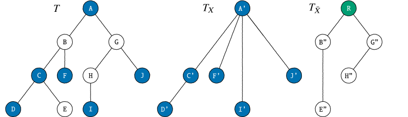
Figure 1: Tree extraction. Original tree (left), extracted tree $T_{X}$ (middle), and extraction of the complement of $X,$ tree $T_{\bar{X}}$ (right). The blue shaded nodes in $T$ form the set $X.$ In the tree $T_{X},$ node $\mathtt{C^{\prime}}$ corresponds to node $\mathtt{C}$ in the original tree $T$, and node $\mathtt{C^{\prime}}$ in the extracted tree $T_{X}$ is the $T_{X}$-view of nodes $\mathtt{C}$ and $\mathtt{E}$ in the original tree $T.$ Finally, node $\mathtt{C}$ in $T$ is the $T$-source of the node $\mathtt{C^{\prime}}$ in $T_{X}.$ Extraction of the complement, $T_{\bar{X}},$ demonstrates the case of adding a dummy root $\mathtt{R}.$

Compact representations of ordinal trees.

Compact representations of ordinal trees is a well-researched area, mainstream methodologies including balanced parentheses (BP) [30, 35, 20, 33, 34], depth-first unary degree sequence (DFUDS) [11, 21, 31], level-order unary degree sequence (LOUDS) [30, 17], and tree covering (TC) [21, 25, 18]. Of these, BP-based representations “combine good time- and space-performance with rich functionality” in practice [8], and we use BP in our solutions. BP is a way of linearising the tree by emitting “(” upon first entering a node and “)” upon exiting, having explored all its descendants during the preorder traversal of the tree. For example, (((()())())((())())) would be a BP-sequence for the tree $T$ in Figure 1.

As shown in [35, 33, 34], an ordinal tree $T$ on $n$ nodes can be represented in $2n+\mathchoice{{\scriptstyle\mathcal{O}}}{{\scriptstyle\mathcal{O}}}{{\scriptscriptstyle\mathcal{O}}}{\scalebox{0.7}{$\scriptscriptstyle\mathcal{O}$}}(n)$ bits of space to support the following operations in $\mathcal{O}(1)$ time, for any node $x\in T:$ $\mathtt{child}(T,x,i)$, the $i$-th child of $x$; $\mathtt{depth}(T,x)$, the number of ancestors of $x$; $\mathtt{LCA}(T,x,y)$, the lowest common ancestor of nodes $x,y\in T;$ and $\mathtt{level\_anc}(T,x,i)$, the $i^{th}$ lowest ancestor of $x.$

Tree extraction.

Tree extraction [28] selects a subset $X$ of nodes while maintaining the underlying hierarchical relationship among the nodes in $X$. Given a subset $X$ of tree nodes called extracted nodes, an extracted tree $T_{X}$ can be obtained from the original tree $T$ through the following procedure. Let $v\notin X$ be an arbitrary node. The node $v$ and all its incident edges in $T$ are removed from $T,$ thereby exposing the parent $p$ of $v$ and $v^{\prime}$s children, $v_{1},v_{2},\ldots,v_{k}.$ Then the nodes $v_{1},v_{2},\ldots,v_{k}$ (in this order) become new children of $p,$ occupying the contiguous segment of positions starting from the (old) position of $v.$ After thus removing all the nodes $v\notin X,$ we have $T_{X}\equiv F_{X},$ if the forest $F_{X}$ obtained is a tree; otherwise, a dummy root $r$ holds the roots of the trees in $F_{X}$ (in the original left-to-right order) as its children. (The symmetry between $X$ and $\bar{X}=V\setminus{}X$ brings about the complement $T_{\bar{X}}$ of the extracted tree $T_{X}.$) An original node $x\in X$ of $T$ and its copy, $x^{\prime}$, in $T_{X}$ are said to correspond to each other; also, $x^{\prime}$ is the $T_{X}$-view of $x,$ and $x$ is the T-source of $x^{\prime}.$ The $T_{X}$-view of a node $y\in T$ ($y$ is not necessarily in $X$) is generally defined to be the node $y^{\prime}\in T_{X}$ corresponding to the lowest node in $\mathcal{A}(y)\cap{}X.$ In this paper, tree extraction is predominantly used to classify nodes into categories, and the labels assigned indicate the weight ranges the original weights belong to.

Figure 1 gives an example of an extracted tree, views and sources.

3 Data Structures for Path Queries

This section gives the design details of the whp and ext data structures.

3.1 Data structures based on heavy-path decomposition

We now describe the approach of [40], which is based on heavy-path decomposition [43].

Heavy-path decomposition (HPD) imposes a structure on a tree. In HPD, for each non-leaf node, a heavy child is defined as the child whose subtree has the maximum cardinality. HPD of a tree $T$ with root $r$ is a collection of disjoint chains, first of which is obtained by always following the heavy child, starting from $r,$ until reaching a leaf. The subsequent chains are obtained by the same procedure, starting from the non-visited nodes closest to the root (ties broken arbitrarily). The crucial property is that any root-to-leaf path in the tree encounters $\mathcal{O}(\lg{n})$ distinct chains. A chain’s head is the node of the chain that is closest to the root; a chain’s tail is therefore a leaf.

Patil et al. [40] used HPD to decompose a path query into $\mathcal{O}(\lg{n})$ queries in sequences. To save space, they designed the following data structure to represent the tree and its HPD. If $x$ is the head of a chain $\phi$, all the nodes in $\phi$ have a (conceptual) reference pointing to $x,$ while $x$ points to itself. A reference count of a node $x$ (denoted as ${rc_{x}}$) stands for the number of times a node serves as a reference. Obviously, only heads feature non-zero reference counts – precisely the lengths of their respective chain. The reference counts of all the nodes are stored in unary in preorder in a bitmap $B=10^{rc_{1}}10^{rc_{2}}\ldots{}10^{rc_{n}}$ using $2n+\mathchoice{{\scriptstyle\mathcal{O}}}{{\scriptstyle\mathcal{O}}}{{\scriptscriptstyle\mathcal{O}}}{\scalebox{0.7}{$\scriptscriptstyle\mathcal{O}$}}(n)$ bits. Then, one has that $rc_{x}=\mathtt{rank_{0}(B,select_{1}(B,x+1))-rank_{0}(B,select_{1}(B,x))}.$ The topology of the original tree $T$ is represented succinctly in another $2n+\mathchoice{{\scriptstyle\mathcal{O}}}{{\scriptstyle\mathcal{O}}}{{\scriptscriptstyle\mathcal{O}}}{\scalebox{0.7}{$\scriptscriptstyle\mathcal{O}$}}(n)$ bits. In addition, they encode the HPD structure of $T$ using a new tree $T^{\prime}$ that is obtained from $T$ via the following transformation. All the non-head nodes become leaves and are directly connected to their respective heads; the heads themselves (except the root) become children of the references of their original parents. All these connections are established respecting the preorder ranks of the nodes in the original tree $T.$ Namely, a node farther from the head attaches to it only after the higher-residing nodes of the chain have done so. This transformation preserves the original preorder ranks. On $T^{\prime},$ operation ref(x) is supported, which returns the head of chain to which the node $x$ in the original tree belongs.

To encode weights they call $C_{x}$ the weight-list of $x$ if it collects, in preorder, all the nodes for which $x$ is a reference. Thus, a non-head node’s list is empty; a head’s list spells the weights in the relevant chain. Define $C=C_{1}C_{2}\ldots{}C_{n}.$ Then, in $C,$ the weight of $x\in T$ resides at position

$$\mathtt{1+select_{1}(B,ref(x))-ref(x)+depth(x)-depth(ref(x))}$$ (1)

(where $\mathtt{depth(x)}$ and $\mathtt{ref(x)}$ are provided by $T$ and $T^{\prime},$ respectively). $C$ is then encoded in a wavelet tree (WT). To answer a query, $T,$ $T^{\prime},$ $B,$ and Equation 1 are used to partition the query path into $\mathcal{O}(\lg{n})$ sub-chains that it overlaps in HPD; and for each sub-chain, one computes the interval in $C$ storing the weights of the nodes in the chain. $I_{m}$ denotes the set of intervals computed. Precisely, for a node $x$, one uses $B$ to find out whether $x$ is the head of its chain; if not, the parent of $x$ in $T^{\prime}$ returns one (say, $y$). Then Equation 1 maps the path $A_{x,y}$ to its corresponding interval in $C.$ One proceeds to the next chain by fetching the (original) parent of $y$, using $T.$ Then, the WT is queried with $\mathcal{O}(\lg{}n)$ simultaneous (i) range quantile (for PM); or (ii) orthogonal range $2d$ queries (for PC and PR).

Range quantile query over a collection of ranges is accomplished via a straightforward extension of the algorithm of Gagie et al. [19]. One descends the wavelet tree $W_{C}$ maintaining a set of current weights $[a,b]$ (initially $[\sigma]$), the current node $v$ (initially the root of $W_{C}$), and $I_{m}.$ When querying the current node $v$ of $W_{C}$ with an interval $[l_{j},r_{j}]\in I_{m},$ one finds out, in $\mathcal{O}(1)$ time, how many weights in the interval are lighter than the mid-point $c$ of $[a,b],$ and how many of them are heavier. The sum of these values then determines which subtree of $W_{C}$ to descend to. There being $\mathcal{O}(\lg\sigma)$ levels in $W_{C}$, and spending $\mathcal{O}(1)$ time for each segment in $I_{m},$ the overall running time is $\mathcal{O}(\lg{n}\lg\sigma).$ PC/PR proceed by querying each interval, independently of the others, with the standard $2d$ search over $W_{C}$.

3.2 Data structures based on tree extraction

The solution by He et al. [28] is based on performing a hierarchy of tree extractions, as follows. One starts with the original tree $T$ weighted over $[\sigma]$, and extracts two trees $T_{0}=T_{1,m}$ and $T_{1}=T_{m+1,\sigma},$ respectively associated with the intervals $I_{0}=[1,m]$ and $I_{1}=[m+1,\sigma],$ where $m=\lfloor\frac{1+\sigma}{2}\rfloor.$ Then both $T_{0}$ and $T_{1}$ are subject to the same procedure, stopping only when the current tree is weight-homogeneous. We refer to the tree we have started with as the outermost tree.

The key insight of tree extraction is that the number of nodes $n^{\prime}$ with weights from $I_{0}$ on the path from $u$ to $v$ equals $\mathtt{n^{\prime}=depth_{0}(u_{0})+depth_{0}(v_{0})-2\cdot{}depth_{0}(z_{0})+\mathbf{1}_{w(z)\in I_{0}}},$ where $\mathtt{depth_{0}(\cdot{})}$ is the depth function in $T_{0},$ $z=LCA(u,v),$ $u_{0},v_{0},z_{0}$ are the $T_{0}$-views of $u,v,$ and $z,$ and $\mathbf{1}_{pred}$ is $1$ if predicate $pred$ is true, and $0$ otherwise. The key step is then, for a given node $x$, how to efficiently find its $0/1$-parent, whose purpose is analogous to a rank-query when descending down the WT. Consider a node $x\in T$ and its ${T_{0}}$-view $x_{0}.$ The corresponding node $x^{\prime}\in T$ of $x_{0}\in T_{0}$ is then called $0$-parent of $x.$ The ${1}$-parent is defined analogously. Supporting $0/1$-parents in compact space is one of the main implementation challenges of the technique, as storing the views explicitly is space-expensive. In [28], the hierarchy of extractions is done by dividing the range not to $2$ but $f=\mathcal{O}(\lg^{\epsilon}{n})$ parts, with $0<\epsilon<1$ being a constant. They classify the nodes according to weights using these $f=\lceil\lg^{\epsilon}{n}\rceil$ labels and use tree covering to represent the tree with small labels in order to find $T_{\alpha}$-views for arbitrary $\alpha\in[\sigma],$ in constant time. They also use this representation to identify, in constant time, which extractions to explore. Therefore, at each of the $\mathcal{O}(\lg{\sigma}/\lg\lg{n})$ levels of the hierarchy of extractions, constant time work is done, yielding an $\mathcal{O}(\lg{\sigma}/\lg\lg{n})$-time algorithm for PC. Space-wise, it is shown that each of the $\mathcal{O}(\lg\sigma/\lg\lg{n})$ levels can be stored in $2n+nH_{0}(W)+\mathchoice{{\scriptstyle\mathcal{O}}}{{\scriptstyle\mathcal{O}}}{{\scriptscriptstyle\mathcal{O}}}{\scalebox{0.7}{$\scriptscriptstyle\mathcal{O}$}}(n\lg\sigma)$ bits of space in total (where $W$ is the multiset of weights on the level) which, summed over all the levels, yields $nH_{0}(W_{T})+\mathcal{O}(n\lg\sigma/\lg\lg{n})$ bits of space. The components of this optimal result, however, use word-parallel techniques that are unlikely to be practical. In addition, one of the components, tree covering (TC) for trees labeled over $[\sigma],\,\sigma=\mathcal{O}(\lg^{\epsilon}{n})$ has not been implemented and experimentally evaluated even for unlabeled versions thereof. Finally, lookup tables for the word-RAM data structures may either be rendered too heavy by word alignment, or too slow by the concomitant arithmetic for accessing its entries. In practice, small blocks of data are usually explicitly scanned [8]. However, we can see no fast way to scan small labeled trees. At the same time, a generic multi-parentheses approach [37] would spare the effort altogether, immediately yielding a $4n\lg\sigma+2n+\mathchoice{{\scriptstyle\mathcal{O}}}{{\scriptstyle\mathcal{O}}}{{\scriptscriptstyle\mathcal{O}}}{\scalebox{0.7}{$\scriptscriptstyle\mathcal{O}$}}(n\lg\sigma)$-bit encoding of the tree, with $\mathcal{O}(1)$-time support for $0/1$-parents. We achieve instead $3n\lg\sigma+\mathchoice{{\scriptstyle\mathcal{O}}}{{\scriptstyle\mathcal{O}}}{{\scriptscriptstyle\mathcal{O}}}{\scalebox{0.7}{$\scriptscriptstyle\mathcal{O}$}}(n\lg\sigma)$ bits of space, as we proceed to describe next.

We store $2n+\mathchoice{{\scriptstyle\mathcal{O}}}{{\scriptstyle\mathcal{O}}}{{\scriptscriptstyle\mathcal{O}}}{\scalebox{0.7}{$\scriptscriptstyle\mathcal{O}$}}(n)$ bits as a regular BP-structure $S$ of the original tree, in which a 1-bit represents an opening parenthesis, and a 0-bit represents a closing one, and mark in a separate length-$n$ bitmap $B$ the types (i.e. whether it is a $0$- or $1$-node) of the $n$ opening parentheses in $S.$ The type of an opening parenthesis at position $i$ in $S$ is thus given by $\mathtt{access(B,rank_{1}(S,i))}.$ Given $S$ and $B$, we find the $t\in\{0,1\}$-parent of $v$ with an approach described in [27]. For completeness, we outline in Algorithm 1 how to locate the $T_{t}$-view of a node $v.$

Algorithm 1 Locate the view of $v\in T$ in $T_{t}$, where $T_{t}$ is the extraction from $T$ of the $t$-nodes

1:$t\in\{0,1\}$

2:function view_of($v,t$)

3:     if $\mathtt{B[v]==t}$ then $\triangleright$ $v$ is a $t$-node itself

4:         return $\mathtt{B.rank_{t}(v)}$      

5:     $\mathtt{\lambda}$ $\leftarrow$ $\mathtt{rank_{t}(B,v)}$ $\triangleright$ how many $t$-nodes precede $v$?

6:     if $\mathtt{\lambda==0}$ then

7:         return null      

8:     $\mathtt{u}$ $\leftarrow$ $\mathtt{select_{t}(B,\lambda)}$ $\triangleright$ find the $\lambda^{th}$ $t$-node

9:     if $\mathtt{LCA(u,v)==u}$ then

10:         return $\mathtt{B.rank_{t}(u)}$      

11:     $\mathtt{z}$ $\leftarrow$ $\mathtt{LCA(u,v)}$ $\triangleright$ $z$ is $LCA$ of a $t$-node $u$ and a non-$t$-node $v$

12:     if $\mathtt{z==null}$ or $\mathtt{B[z]==t}$ then $\triangleright$ $z$ is a $t$-node $\Rightarrow\nexists$ $t$-parent closer to $v$

13:         return $\mathtt{B.rank_{t}(z)}$ $\triangleright$ or null      

14:     $\mathtt{\lambda}$ $\leftarrow$ $\mathtt{rank_{t}(B,z)}$ $\triangleright$ how many $t$-nodes precede $z$?

15:     $\mathtt{r}$ $\leftarrow$ $\mathtt{select_{t}(B,\lambda+1)}$ $\triangleright$ the first $t$-descendant of $z$

16:     $\mathtt{z_{t}}$ $\leftarrow$ $\mathtt{rank_{t}(B,r)}$ $\triangleright$ $z_{t}$ is the $T_{t}$-view of $r$

17:     $\mathtt{p}$ $\leftarrow$ $\mathtt{T_{t}.parent(z_{t})}$ $\triangleright$ $p$ can be null if $z_{t}$ is $0$

18:     return $\mathtt{p}$

First, find the number of $t$-nodes preceding $v$ (line 5). If none exists (line 6), we are done; otherwise, let $u$ be the $t$-node immediately preceding $v$ (line 8). If $u$ is an ancestor of $v,$ it is the answer (line 10); else, set $z=LCA(u,v).$ If $z$ is a $t$-node, or non-existent (because the tree is actually a forest), then return $z$ or null, respectively. Otherwise ($z$ exists and not a $t$-node), in line 15 we find the first $t$-descendant $r$ of $z$ (it exists because of $u$). This descendant cannot be a parent of $v,$ since otherwise we would have found it before. It must share though the same $t$-parent with $v.$ We map this descendant to a node $z_{t}$ in $T_{t}$ (line 16). Finally, we find the parent of $z_{t}$ in $T_{t}$ (line 17).

The combined cost of $S$ and $B$ is $2n+n+\mathchoice{{\scriptstyle\mathcal{O}}}{{\scriptstyle\mathcal{O}}}{{\scriptscriptstyle\mathcal{O}}}{\scalebox{0.7}{$\scriptscriptstyle\mathcal{O}$}}(n)=3n+\mathchoice{{\scriptstyle\mathcal{O}}}{{\scriptstyle\mathcal{O}}}{{\scriptscriptstyle\mathcal{O}}}{\scalebox{0.7}{$\scriptscriptstyle\mathcal{O}$}}(n)$ bits. At each of the $\lg\sigma$ levels of extraction, we encode $0/1$-labeled trees in the same way, so the total space is $3n\lg\sigma+\mathchoice{{\scriptstyle\mathcal{O}}}{{\scriptstyle\mathcal{O}}}{{\scriptscriptstyle\mathcal{O}}}{\scalebox{0.7}{$\scriptscriptstyle\mathcal{O}$}}(n\lg\sigma)$ bits.

Query algorithms in the ext data structure proceed within the generic framework of extracting $T_{0}$ and $T_{1}.$ Let $n^{\prime}=|P_{u_{0},v_{0}}|.$ In PM, we recurse on $T_{0}$ if $k<n^{\prime},$ for a query that asks for a node with the $k^{th}$ smallest weight on the path $P_{u_{0},v_{0}};$ otherwise, we recurse on $T_{1}$ with $k\leftarrow k-n^{\prime}$ and $u_{1},\,v_{1}.$ We stop upon encountering a tree with homogeneous weights. This logic is embodied in Algorithm 2 in Appendix A. Theoretical running time is $\mathcal{O}(\lg\sigma)$, as all the primitives used are $\mathcal{O}(1)$-time.

A procedure for the PC and PR is essentially similar to that for the PM problem. We maintain two nodes, $u$ and $v,$ as the query nodes with respect to the current extraction $T$, and a node $z$ as the lowest common ancestor of $u$ and $v$ in the current tree $T.$ Initially, $u,v\in T$ are the original query nodes, and $T$ is the outermost tree. Correspondingly, $z$ is the LCA of the nodes $u$ and $v$ in the original tree; we determine the weight of $z$ and store it in $w,$ which is passed down the recursion. Let $[a,b]$ be the query interval, and $[p,q]$ be the current range of weights of the tree. Initially, $[p,q]=[\sigma].$ First, we check whether the current interval $[p,q]$ is contained within $[a,b].$ If so, the entire path $A_{u,z}\cup{}A_{v,z}$ belongs to the answer. Here, we also check whether $w\in[a,b].$ Then we recurse on $T_{t}$ ($t\in\{0,1\}$) having computed the corresponding $T_{t}$-views of the nodes $u,v,$ and $z,$ and with the corresponding current range. The full details of the $\mathcal{O}(\lg\sigma)$-time algorithm are given in Algorithm 3 of Appendix A.

To summarize, the variant of ext that we design here uses $3n\lg\sigma+\mathchoice{{\scriptstyle\mathcal{O}}}{{\scriptstyle\mathcal{O}}}{{\scriptscriptstyle\mathcal{O}}}{\scalebox{0.7}{$\scriptscriptstyle\mathcal{O}$}}(n\lg\sigma)$ bits to support PM and PC in $\mathcal{O}(\lg\sigma)$ time, and PR in $\mathcal{O}((1+\kappa)\lg\sigma)$ time. Compared to the original succinct solution [28] based on tree extraction, our variant uses about $3$ times the space with a minor slow-down in query time, but is easily implementable using bitmaps and BP, both of which have been studied experimentally (see e.g. [8] and [37] for an extensive review).

4 Experimental Results

We now conduct experimental studies on data structures for path queries.

	Symbol	Description
pointer-based	nv	Naïve data structure in Section 4.1
	${\mathtt{nv^{L}}}$	Naïve data structure in Section 4.1, augmented with $\mathcal{O}(1)$ query-time $LCA$ of [10]
	${\mathtt{ext^{\dagger}}}$	A solution based on tree extraction [28] in Section 2
	${\mathtt{whp^{\dagger}}}$	A non-succinct version of the wavelet tree- and heavy-path decomposition-based solution of [40] in Section 3.
	${\mathtt{nv^{c}}}$	Naïve data structure of Section 4.1, using succinct data structures to represent the tree structure and weights
succinct	${\mathtt{ext^{c}}}$	$3n\lg\sigma+\mathchoice{{\scriptstyle\mathcal{O}}}{{\scriptstyle\mathcal{O}}}{{\scriptscriptstyle\mathcal{O}}}{\scalebox{0.7}{$\scriptscriptstyle\mathcal{O}$}}(n\lg\sigma)$-bits-of-space scheme for tree extraction of Section 3.2, with compressed bitmaps
	${\mathtt{ext^{p}}}$	$3n\lg\sigma+\mathchoice{{\scriptstyle\mathcal{O}}}{{\scriptstyle\mathcal{O}}}{{\scriptscriptstyle\mathcal{O}}}{\scalebox{0.7}{$\scriptscriptstyle\mathcal{O}$}}(n\lg\sigma)$-bits-of-space scheme for tree extraction of Section 3.2, with uncompressed bitmaps
	${\mathtt{whp^{c}}}$	Succinct version of whp, with compressed bitmaps
	${\mathtt{whp^{p}}}$	Succinct version of whp, with uncompressed bitmaps

Table 1: The implemented data structures and the abbreviations used to refer to them.

4.1 Implementation

For ease of reference, we outline the data structures implemented in Table 1.

Naïve approaches (both plain pointer-based nv/${\mathtt{nv^{L}}}$ and succinct ${\mathtt{nv^{c}}}$) resolve a query on the path $P_{x,y}$ by explicitly traversing it from $x$ to $y$. At each encountered node, we either (i) collect its weight into an array (for PM); (ii) check if its weight is in the query range (for PC); (iii) if the check in (ii) succeeds, we collect the node into a container (for PR). In PM, we subsequently call a standard introspective selection algorithm [36] over the array of collected weights. Depths and parent pointers, explicitly stored at each node, guide in upwards traversal from $x$ and $y$ to their common ancestor. Plain pointer-based tree topologies are stored using forward-star [6] representation. In ${\mathtt{nv^{L}}}$, we equip nv with the linear-space and $\mathcal{O}(1)$-time LCA-support structure of [10].

Succinct structures ${\mathtt{ext^{c}}}$/${\mathtt{ext^{p}}}$/${\mathtt{whp^{c}}}$/${\mathtt{whp^{p}}}$ are implemented with the help of the succinct data structures library sdsl-lite of Gog et al. [22]. To implement whp and the practical variant of ext we designed in Section 3.2, two types of bitmaps are used: a compressed bitmap [41] (implemented in sdsl::rrr_vector of sdsl-lite) and plain bitmap (implemented in sdsl::bit_vector of sdsl-lite). For ${\mathtt{nv^{c}}}$, the weights are stored using $\lceil\lg\sigma\rceil$ bits each in a sequence and the structure theoretically occupies $2n+n\lg\sigma+\mathchoice{{\scriptstyle\mathcal{O}}}{{\scriptstyle\mathcal{O}}}{{\scriptscriptstyle\mathcal{O}}}{\scalebox{0.7}{$\scriptscriptstyle\mathcal{O}$}}(n\lg\sigma)$ bits. For uniformity, across our data structures, tree navigation is provided solely by a BP representation based on [21] (implemented in sdsl::bp_support_gg), chosen on the basis of our benchmarks.

Plain pointer-based implementation ${\mathtt{ext^{\dagger}}}$ is an implementation of the solution by He et al. [28] for the pointer-machine model, which uses tree extraction. In it, the views $x_{0}\in T_{0},\,x_{1}\in T_{1}$ for each node that arises in the hierarchy of extractions, as well as the depths in $T,$ are explicitly stored. Similarly, ${\mathtt{whp^{\dagger}}}$ is a plain pointer-based implementation of the data structure by Patil et al. [40]. The relevant source code is accessible at https://github.com/serkazi/tree_path_queries.

4.2 Experimental setup

	num nodes	diameter	$\sigma$	$\log{\sigma}$	$H_{0}$	Description
eu.mst.osm	27,024,535	109,251	121,270	16.89	9.52	An MST we constructed over map of Europe [39]
eu.mst.dmcs	18,010,173	115,920	843,781	19.69	8.93	An MST we constructured over European road network [1]
eu.emst.dem	50,000,000	175,518	5020	12.29	9.95	An Euclidean MST we constructed over DEM of Europe [4]
mrs.emst.dem	30,000,000	164,482	29,367	14.84	13.23	An Euclidean MST we constructed over DEM of Mars [3]

Table 2: Datasets metadata. DEM stands for Digital Elevation Model, and MST for minimum spanning tree. Weights are over $\{0,1,\ldots,\sigma-1\},$ and $H_{0}$ is the entropy of the multiset of weights. In DEM, elevation (in meters) is used as weights. For eu.mst.osm, distance in meters between locations, and for eu.mst.dmcs, travel time between locations, for a proprietary “car” profile in tenths of a second, are used as weights.

The platform used is a $128$GiB RAM, Intel(R) Xeon(R) Gold $6234$ CPU $3.30$GHz server running 4.15.0-54-generic 58-Ubuntu SMP x86_64 kernel. The build is due to clang-8 with -g,-O2,
-std=c++17,mcmodel=large,-NDEBUG flags. Our datasets originate from geographical information systems (GIS). In Table 2, the relevant meta-data on our datasets is given.

We generated query paths by choosing a pair uniformly at random (u.a.r.). To generate a range of weights, $[a,b],$ we follow the methodology of [16] and consider large, medium, and small configurations: given $K,$ we generate the left bound $a\in[W]$ u.a.r., whereas $b$ is generated u.a.r. from $[a,a+\lceil\frac{W-a}{K}\rceil].$ We set $K=1,10,$ and $100$ for respectively large, medium, and small. To counteract skew in weight distribution in some of the datasets, when generating the weight-range $[a,b]$, we in fact generate a pair from $[n]$ rather than $[\sigma]$ and map the positions to the sorted list of input-weights, ensuring the number of nodes covered by the generated weight-range to be proportional to $K^{-1}.$

4.3 Space performance and construction costs

A single data structure we implement (be it ever nv-, ext-, or whp-family), taken individually, answers all three types of queries (PM, PC, and PR). Hence, we consider space consumption first.

	Dataset	nv	${\mathtt{nv^{L}}}$	${\mathtt{whp^{\dagger}}}$	${\mathtt{ext^{\dagger}}}$	${\mathtt{nv^{c}}}$	${\mathtt{ext^{c}}}$	${\mathtt{ext^{p}}}$	${\mathtt{whp^{c}}}$	${\mathtt{whp^{p}}}$
space	eu.mst.osm	406.3	972.1	3801	5943	21.71	59.85	75.74	21.71	34.42
	eu.mst.dmcs	406.4	974.0	4274	6768	34.46	82.16	106.0	29.69	48.77
	eu.emst.dem	394.1	988.5	3342	4613	19.64	45.41	59.15	19.64	31.66
	mrs.emst.dem	386.7	1005	3579	5383	17.35	51.71	66.02	17.35	28.80
peak/time	eu.mst.osm	491.0/1	987.9/5	3785/28	9586/47	21.71/1	295.0/23	295.0/23	1347/62	1347/61
	eu.mst.dmcs	439.8/1	1002/4	4403/19	12382/37	29.69/1	399.7/18	399.7/18	1360/42	1360/42
	eu.emst.dem	401.0/2	1021/10	3460/47	5286/67	19.64/1	287.6/32	287.6/32	1333/115	1333/115
	mrs.emst.dem	392.4/1	1016/5	3719/30	6027/46	17.35/1	269.3/22	269.3/22	1337/69	1337/69

Table 3: (upper) Space occupancy of our data structures, in bits per node, when loaded into memory; (lower) peak memory usage (m in bits per node) during construction and construction time ($t$ in seconds) shown as $\mathbf{m}/t$.

The upper part of the Table 3 shows the space usage of our data structures. The structures nv/${\mathtt{nv^{L}}}$ are lighter than ${\mathtt{ext^{\dagger}}}$/${\mathtt{whp^{\dagger}}}$, as expected. Adding fast $LCA$ support doubles the space requirement for nv, whereas succinctness (${\mathtt{nv^{c}}}$) uses up to $20$ times less space than nv. The difference between ${\mathtt{ext^{\dagger}}}$ and ${\mathtt{whp^{\dagger}}}$, in turn, is in explicit storage of the $0$-views for each of the $\Theta(n\lg\sigma)$ nodes occurring during tree extraction. In ${\mathtt{whp^{\dagger}}}$, by contrast, $\mathtt{rank}_{0}$ is induced from $\mathtt{rank}_{1}$ (via subtraction) – hence the difference in the empirical sizes of the otherwise $\Theta(n\lg\sigma)$-word data structures.

The succinct ${\mathtt{nv^{c}}}$’s empirical space occupancy is close to the information-theoretic minimum given by $\lg\sigma+2$ (Table 2). The structures ${\mathtt{ext^{c}}}$/${\mathtt{ext^{p}}}$ occupy about three times as much, which is consistent with the design of our practical solution (Section 3.2). It is interesting to note that the data structure ${\mathtt{whp^{c}}}$ occupies space close to bare succinct storage of the input alone (${\mathtt{nv^{c}}}$). Entropy-compression significantly impacts both families of succinct structures, whp and ext, saving up to $20$ bits per node when switching from plain bitmap to a compressed one. Compared to pointer-based solutions (nv/${\mathtt{nv^{L}}}$/${\mathtt{whp^{\dagger}}}$/${\mathtt{ext^{\dagger}}}$), we note that ${\mathtt{ext^{c}}}$/${\mathtt{ext^{p}}}$/${\mathtt{whp^{c}}}$/${\mathtt{whp^{p}}}$ still allow usual navigational operations on $T$, whereas the former shed this redundancy, to save space, after preprocessing.

Overall, the succinct ${\mathtt{whp^{p}}}$/${\mathtt{whp^{c}}}$/${\mathtt{ext^{p}}}$/${\mathtt{ext^{c}}}$ perform very well, being all well-under $1$ gigabyte for the large datasets we use. This suggests scalability: when trees are so large as not to fit into main memory, it is clear that the succinct solutions are the method of choice.

The lower part in Table 3 shows peak memory usage (m, in bits per node) and construction time (t, in seconds), as $\mathbf{m}/t.$ The structures ${\mathtt{ext^{p}}}$/${\mathtt{ext^{c}}}$ are about three times faster than ${\mathtt{whp^{p}}}$/${\mathtt{whp^{c}}}$ to build, and use four times less space at peak. This is expected, as whp builds two different structures (HPD and then WT). This is reversed for ${\mathtt{ext^{\dagger}}}$/${\mathtt{whp^{\dagger}}}$; time-wise, as ${\mathtt{ext^{\dagger}}}$ performs more memory allocations during construction (although our succinct structures are flattened into a heap layout, ${\mathtt{ext^{\dagger}}}$ stores pointers to $T_{0}/T_{1}$; this is less of a concern for ${\mathtt{whp^{\dagger}}}$, whose very purpose is tree linearisation).

	Dataset	nv	${\mathtt{nv^{L}}}$	${\mathtt{ext^{\dagger}}}$	${\mathtt{whp^{\dagger}}}$	${\mathtt{nv^{c}}}$	${\mathtt{ext^{c}}}$	${\mathtt{ext^{p}}}$	${\mathtt{whp^{c}}}$	${\mathtt{whp^{p}}}$
median	eu.mst.osm	658	475	4.22	6.10	7078	85.3	51.1	111	51.2
	eu.mst.dmcs	566	412	5.16	6.28	6556	84.6	54.8	120	54.7
	eu.emst.dem	710	436	4.44	5.10	9404	106	81.9	96.7	54.9
	mrs.emst.dem	472	298	4.93	4.53	7018	124	97.0	88.3	49.5
counting	eu.mst.osm	238	140	6.88	18.4	3553	247	167	139	56.9	large
	eu.mst.dmcs	204	121	7.31	19.7	3300	253	178	142	57.3
	eu.emst.dem	338	195	5.97	11.5	4835	215	168	105	55.9
	mrs.emst.dem	232	174	5.25	8.40	3614	206	164	91	49.3
	eu.mst.osm	244	143	5.47	17.8	3555	213	146	129	54.2	medium
	eu.mst.dmcs	209	124	6.94	18.4	3297	224	160	133	56.5
	eu.emst.dem	339	195	4.55	10.0	4840	178	140	100	54.9
	mrs.emst.dem	237	143	5.91	8.74	3613	199	154	89.7	48.9
	eu.mst.osm	239	139	5.25	15.4	3551	190	132	119	53.9	small
	eu.mst.dmcs	209	123	5.25	18.9	3300	206	148	126	55.2
	eu.emst.dem	347	200	3.92	9.34	4832	154	124	94.9	53.2
	mrs.emst.dem	238	144	4.82	7.41	3615	178	133	84.2	47.6

Table 4: Average time to answer a query, from a fixed set of $10^{6}$ randomly generated path median and path counting queries, in microseconds. Path counting queries are given in large, medium, and small configurations.

4.4 Path median queries

The upper section of Table 4 records the mean time for a single median query (in $\mathrm{\SIUnitSymbolMicro s}$) averaged over a fixed set of $10^{6}$ randomly generated queries.

Succinct structures ${\mathtt{whp^{c}}}$/${\mathtt{whp^{p}}}$/${\mathtt{ext^{c}}}$/${\mathtt{ext^{p}}}$ perform well on these queries, with a slow-down of at most $20$-$30$ times from their respective pointer-based counterparts. Using entropy-compression degrades the speed of whp almost twice. Overall, the families whp and ext seem to perform at the same order of magnitude. This is surprising, as in theory whp should be a factor of ${\lg{n}}$ slower. The discrepancy is explained partly by small average number of segments in HPD, averaging $9\pm{}2$ for our queries. (The number of unary-degree nodes in our datasets is $35\%$-$56\%,$ which makes smaller number of heavy-path segments prevalent. We did not use trees with few unary-degree nodes in our experiments, as the height of such trees are not large enough to make constructing data structures for path queries worthwhile.) When the queries are partitioned by the number of chains in the HPD, the curves for ${\mathtt{ext^{c}}}$/${\mathtt{ext^{p}}}$ stay flat whereas those for ${\mathtt{whp^{c}}}$/${\mathtt{whp^{p}}}$ grow linearly (see Figure 3 in Appendix B). Take eu.mst.dmcs as an example. When the query path is partitioned into $9$ chains, ${\mathtt{ext^{p}}}$ is only slightly faster than ${\mathtt{whp^{p}}}$, but when the query path contains $19$ chains, ${\mathtt{ext^{p}}}$ is about $2.3$ times so. This suggests to favour the ext family over whp whenever performance in the worst case is important. Furthermore, navigational operations in ${\mathtt{ext^{p}}}$/${\mathtt{ext^{c}}}$ and ${\mathtt{whp^{p}}}$/${\mathtt{whp^{c}}}$, despite of similar theoretical worst-case guarantees, involve different patterns of using the rank/select primitives. For one, ${\mathtt{whp^{p}}}$/${\mathtt{whp^{c}}}$ does not call $LCA$ during the search – mapping of the search ranges when descending down the recursion is accomplished by a single rank call, whereas ${\mathtt{ext^{p}}}$/${\mathtt{ext^{c}}}$ computes $LCA$ at each level of descent (for its its own analog of rank – the view computation in Algorithm 1). Now, $LCA$ is a non-trivial combination of rank/select calls. The difference between ${\mathtt{ext^{p}}}$/${\mathtt{ext^{c}}}$ and ${\mathtt{whp^{p}}}$/${\mathtt{whp^{c}}}$ will therefore become pronounced in a large enough tree; with tangible HPD sizes, the constants involved in (albeit theoretically $\mathcal{O}(1)$) $LCA$ calls are overcome by $\lg{n}.$

Naïve structures nv/${\mathtt{nv^{L}}}$/${\mathtt{nv^{c}}}$ are visibly slower in PM than in PC (considered in Section 4.5), as expected — for PM, having collected the nodes encountered, we also call a selection algorithm. In PC, by contrast, neither insertions into a container nor a subsequent search for median are involved. Navigation and weights-uncompression in ${\mathtt{nv^{c}}}$ render it about $10$ times slower than its plain counterpart. The ${\mathtt{nv^{L}}}$ being little less than twice faster than its $LCA$-devoid counterpart, nv, is explained by the latter effectively traversing the query path twice — once to locate the $LCA,$ and again to answer the query proper. Any succinct solution is about $4$-$8$ times faster than the fastest naïve, ${\mathtt{nv^{L}}}$.

4.5 Path counting queries

The lower section in Table 4 records the mean time for a single counting query (in $\mathrm{\SIUnitSymbolMicro s}$) averaged over a fixed set of $10^{6}$ randomly generated queries, for large, medium, and small setups.

Structures nv/${\mathtt{nv^{L}}}$/${\mathtt{nv^{c}}}$ are insensitive to $\kappa,$ as the bottleneck is in physically traversing the path.

Succinct structures ${\mathtt{whp^{p}}}$/${\mathtt{whp^{c}}}$ and ${\mathtt{ext^{p}}}$/${\mathtt{ext^{c}}}$ exhibit decreasing running times as one moves from large to small — as the query weight-range shrinks, so does the chance of branching during the traversal of the implicit range tree. The fastest (uncompressed) ${\mathtt{whp^{p}}}$ and the slowest (compressed) ${\mathtt{ext^{c}}}$ succinct solutions differ by a factor of $4,$ which is intrinsically larger constants in ${\mathtt{ext^{c}}}$’s implementation compounded with slower rank/select primitives in compressed bitmaps, at play. The uncompressed ${\mathtt{whp^{p}}}$ is about $2$-$3$ times faster than ${\mathtt{ext^{p}}}$, the gap narrowing towards the small setup. The slowest succinct structure, ${\mathtt{ext^{c}}}$, is nonetheless competitive with the nv/${\mathtt{nv^{L}}}$ already in large configuration, with the advantage of being insensitive to tree topology.

In ${\mathtt{ext^{\dagger}}}$-${\mathtt{whp^{\dagger}}}$ pair, ${\mathtt{whp^{\dagger}}}$ is $2$-$3$ times slower. This is predictable, as the inherent $\lg{n}$-factor slow-down in ${\mathtt{whp^{\dagger}}}$ is no longer offset by differing memory access patterns – following a pointer “downwards” (i.e. $0/1$-view in ${\mathtt{ext^{\dagger}}}$ and $\mathtt{rank}_{0/1}()$ in ${\mathtt{whp^{\dagger}}}$) each require a single memory access.

Dataset	$\kappa$	nv	${\mathtt{nv^{L}}}$	${\mathtt{ext^{\dagger}}}$	${\mathtt{whp^{\dagger}}}$	${\mathtt{nv^{c}}}$	${\mathtt{ext^{c}}}$	${\mathtt{ext^{p}}}$	${\mathtt{whp^{c}}}$	${\mathtt{whp^{p}}}$
eu.mst.osm	9,840	356	256	184	70.7	3766					large
eu.mst.dmcs	9,163	309	224	147	66.8	3485
eu.emst.dem	14,211	389	241	140	77.5	4926
mrs.emst.dem	10,576	267	178	89.2	55.1	3668
eu.mst.osm	1,093	322	222	43.7	28.8	3706					medium
eu.mst.dmcs	1,090	277	196	34.0	29.7	3434
eu.emst.dem	1,464	354	206	32.1	20.1	4880
mrs.emst.dem	1,392	250	151	22.1	15.6	3639
eu.mst.osm	182	311	212	13.8	19.0	3685	1965	485	795	226	small
eu.mst.dmcs	236	271	193	13.2	21.0	3529	2518	632	1043	292
eu.emst.dem	215	353	203	10.2	12.7	4873	1276	378	590	205
mrs.emst.dem	117	242	145	8.88	9.57	3632	881	278	475	162

Table 5: Average time to answer a path reporting query, from a fixed set of $10^{6}$ randomly generated path reporting queries, in microseconds. The queries are given in large, medium, and small configurations. Average output size for each group is given in column $\kappa.$

4.6 Path reporting queries

Table 5 records the mean time for a single reporting query (in $\mathrm{\SIUnitSymbolMicro s}$) averaged over a fixed set of $10^{6}$ randomly generated queries, for large, medium, and small setups.

Structures ${\mathtt{whp^{c}}}$/${\mathtt{whp^{p}}}$/${\mathtt{ext^{c}}}$/${\mathtt{ext^{p}}}$ recover each reported node’s weight in $\mathcal{O}(\lg\sigma)$ time. Thus, when $\lg{n}\ll\kappa$, the query time for both ext and whp families become $\mathcal{O}(\kappa\cdot{}\log\sigma).$ (At this juncture, a caveat is in order: design of whp’s in Section 3.1 allows a PR-query to only return the index in the array $C$ — not the original preorder identifier of the node, as does the ext.) When $\kappa$ is large, therefore, these structures are not suitable for use in PR, as nv/${\mathtt{nv^{L}}}$/${\mathtt{nv^{c}}}$are clearly superior ($\mathcal{O}((1+\kappa)\lg{n})$ vs $\mathcal{O}(\kappa)$), and we confine the experiments for ${\mathtt{ext^{c}}}$/${\mathtt{ext^{p}}}$/${\mathtt{whp^{c}}}$/${\mathtt{whp^{p}}}$ to the small setup only (bottom-right corner in Table 5).

We observe that the succinct structures ${\mathtt{ext^{p}}}$ and ${\mathtt{whp^{p}}}$ are competitive with nv/${\mathtt{nv^{L}}}$, in small setting: informally, time saved in locating the nodes to report is used to uncompress the nodes’ weights (whereas in nv/${\mathtt{nv^{L}}}$ the weights are explicit). Between the succinct ext and whp, clearly whp is faster, as select() on a sequence as we go up the wavelet tree tend to have lower constant factors than the counterpart operation on BP.

Structures ${\mathtt{whp^{\dagger}}}$ and ${\mathtt{ext^{\dagger}}}$ exhibit same order of magnitude in query time, with the former being sometimes about $2$ times faster on non-small setups. Among two somewhat intertwined reasons, one is that ${\mathtt{whp^{\dagger}}}$ returns an index to the permuted array, as noted above. (Converting to the original id would necessitate an additional memory access.) Secondly, in the implicit range tree during the $2d$ search in ${\mathtt{whp^{\dagger}}}$, when the current range is contained within the query interval, we start reporting the node weights by merely incrementing a counter — position in the WT sequence. By contrast, in such situations ${\mathtt{ext^{\dagger}}}$ iterates through the nodes being reported calling parent() for the current node, which is one additional memory access compared to ${\mathtt{whp^{\dagger}}}$ (at the scale of $\mathrm{\SIUnitSymbolMicro s}$, this matters). Indeed, operations on trees tend to be little more expensive than similar operations on sequences.

Structures nv/${\mathtt{nv^{L}}}$/${\mathtt{nv^{c}}}$ are less sensitive to the query weight range’s magnitude, since they simply scan the path along with pushing into a container. The differences in running time in Table 5 between the configurations are thus accounted for by container operations’ cost. Naïve structures’ query times for PR being dependent solely on the query path’s length, they are unfeasible for large-diameters trees (whereas they may be suitable for shallow ones, e.g. originating from “small-world” networks).

Figure 2: Visualization of some of the entries in Table 4. Inner rectangle magnifies the mutual configuration of the succinct data structures ${\mathtt{whp^{p}}}$,${\mathtt{whp^{c}}}$,${\mathtt{ext^{p}}}$, and ${\mathtt{ext^{c}}}$. The succinct naïve structure ${\mathtt{nv^{c}}}$ is not shown.

Overall evaluation.

We visualize in Figure 2 some typical entries in Table 4 to illustrate the structures clustering along the space/time trade-offs: nv/${\mathtt{nv^{L}}}$ (upper-left corner) are lighter in terms of space, but slow; pointer-based ${\mathtt{ext^{\dagger}}}$/${\mathtt{whp^{\dagger}}}$ are very fast, but space-heavy. Between the two extremes of the spectrum, the succinct structures ${\mathtt{ext^{c}}}$/${\mathtt{ext^{p}}}$/${\mathtt{whp^{c}}}$/${\mathtt{whp^{p}}}$, whose mutual configuration is shown magnified in inner rectangle, are space-economical and yet offer fast query times.

5 Conclusion

We have designed and experimentally evaluated recent algorithmic proposals in path queries in weighted trees, by either faithfully replicating them or offering practical alternatives. Our data structures include both plain pointer-based and succinct implementations. Our succinct realizations are themselves further specialized to be either plain or entropy-compressed.

We measure both query time and space performance of our data structures on large practical sets. We find that the succinct structures we implement offer an attractive alternative to plain pointer-based solutions, in scenarios with critical space- and query time-performance and reasonable tolerance to slow-down. Some of the structures we implement (${\mathtt{whp^{c}}}$) occupy space equal to bare compressed storage (${\mathtt{nv^{c}}}$) of the object and yet offer fast queries on top of it, while another structure (${\mathtt{ext^{c}}}$/${\mathtt{ext^{p}}}$) occupies space comparable to ${\mathtt{nv^{c}}}$, offers fast queries and low peak memory in construction. While whp succinct family performs well in average case, thus offering attractive trade-offs between query time and space occupancy, ext is robust to the structure of the underlying tree, and is therefore recommended when strong worst-case guarantees are vital.

Our design of the practical succinct structure based on tree extraction (ext) results in a theoretical space occupancy of $3n\lg\sigma+\mathchoice{{\scriptstyle\mathcal{O}}}{{\scriptstyle\mathcal{O}}}{{\scriptscriptstyle\mathcal{O}}}{\scalebox{0.7}{$\scriptscriptstyle\mathcal{O}$}}(n\lg\sigma)$ bits, which helps explain its somewhat higher empirical space cost when compared to the succinct whp family. At the same time, verbatim implementation of the space-optimal solution by He et al. [28] draws on components that are likely to be cumbersome in practice. For the path query types considered in this study, therefore, realization of the theoretically time- and space-optimal data structure — or indeed some feasible alternative thereof — remains an interesting open problem in algorithm engineering.

Appendix A Query Algorithms

We enter Algorithm 2 with several parameters – the current tree $T$, the query nodes $u,v$, the $LCA\,\,z$ of the two nodes, the quantile $k$ we are looking for, the weight-range $[a,b],$ and a number $w.$ These are initially set, respectively, to be the outermost tree, the original query nodes, the $LCA$ of the original query nodes, the median’s index (i.e. half the length of the corresponding path in the original tree), the weight range $[\sigma],$ and the weight of the $LCA$ of the original nodes. We maintain the invariant that $T$ is weighted over $[a,b],$ $z$ is the $LCA$ of $u$ and $v$ in $T.$ Line 3 checks whether the current tree is weight-homogeneous. If it is, we immediately return the current weight $a$ (line 4). Otherwise, the quantile value we are looking for is either on the left or on the right half of the weight-range $[a,b].$ In lines 6-12 we check, successively, the ranges $[a_{0},b_{0}]$ and $[a_{1},b_{1}]$ to determine how many nodes on the path from $u$ to $v$ in $T$ have weights from the corresponding interval. The accumulator variable acc keeps track of these values and is certain to always be at most $k.$ When the next value of acc is about to become larger than $k$ (line 12), we are certain that the current weight-interval is the one we should descend to (line 13). The invariants are maintained in line 7: there, we calculate the views of the current nodes $u,v,$ and $z$ in the extracted tree we are looking at.

It is clear that $\mathcal{O}(\lg\sigma)$ levels of recursion are explored. At each level of recursion, a constant number of view_of() and depth() operations are performed (lines 7-8). Hence, assuming the $\mathcal{O}(1)$-time for the latter operations themselves, we have a $\mathcal{O}(\lg\sigma)$ query-time algorithm, overall.

Algorithm 2 Selection: return the $k$-th smallest weight on the path from $u\in T$ to $v\in T$

1:$z=LCA(u,v),\,a\leq b,\,\,k\geq 0$

2:function select($T,u,v,z,k,w,[a..b]$)

3:    if $a==b$ then

4:         return $a$     

5:    $\mathtt{acc}$ $\leftarrow$ $\mathtt{0}$

6:    for $\mathtt{t\in 0..1}$ do

7:         $\mathtt{iu,iv,iz}$ $\leftarrow$ $\mathtt{view\_of(u,t),\,view\_of(v,t),\,view\_of(z,t)}$

8:         $\mathtt{du,dv,dz}$ $\leftarrow$ $\mathtt{depth(B_{t},ix),\,depth(B_{t},iy),\,depth(B_{t},iz)}$

9:         $\mathtt{dw}$ $\leftarrow$ $\mathtt{du+dv-2\cdot{}dz}$

10:         if $\mathtt{a_{t}\leq w\leq b_{t}}$ then $\triangleright$ $[a_{0}..b_{0}]=[a..c],\,\,[a_{1}..b_{1}]=[c+1..b],\,\,c=(a+b)/2$

11:             $\mathtt{dw}$ $\leftarrow$ $\mathtt{dw+1}$          

12:         if $\mathtt{acc+dw>k}$ then

13:             return select($\mathtt{T_{t},iu,iv,iz,k-acc,w,[a_{t}..b_{t}]}$)          

14:         $\mathtt{acc}$ $\leftarrow$ $\mathtt{acc+dw}$     

15:    assert(false); $\triangleright$ unreachable statement – line 13 should execute at some point

Algorithm 3 is adapted from [28], and reasoning similar to Algorithm 2 applies. Now we have a weight-range $[p,q],$ and maintain that $[p,q]\cap{}[a,b]\neq\emptyset$ (the appropriate action is in line 13). In line 3 we check if the query range $[p,q]$ is completely inside the the current range. If so, we return all the nodes (if $report$ argument is set to True) and the number thereof (for counting case). If not, we descend to $T_{0}$ and $T_{1}$ (line 15), as discussed previously. Algorithm 3 emulates traversal of a path in range tree, maintaining the current weight range $[a,b]$ and halving at at each step (line 15). As operations in lines 16 and 17 are constant-time, the algorithm runs in time $\mathcal{O}(\lg{\sigma}).$

Algorithm 3 Counting and reporting.

1:$z=LCA(u,v),\,p\leq q$

2:function countreport($T,u,v,z,w,[p,q],[a,b],vec=null,report=False$)

3:    if $p\leq a\leq b\leq q$ then

4:         if $report$ then

5:             for $\mathtt{pu}\in\mathcal{A}(u)\,\textrm{and}\,\mathtt{pu\neq z}$ do

6:                 $\mathtt{vec}$ $\leftarrow$ $\mathtt{vec+original\_node(pu)}$              

7:             for $\mathtt{pv}\in\mathcal{A}(v)\,\textrm{and}\,\mathtt{pv\neq z}$ do

8:                 $\mathtt{vec}$ $\leftarrow$ $\mathtt{vec+original\_node(pv)}$              

9:             if $a\leq w\leq b$ then

10:                 $\mathtt{vec}$ $\leftarrow$ $\mathtt{vec+original\_node(pv)}$                       

11:         return $\mathtt{depth(u)+depth(v)-2depth(z)+1_{w\in[p,q]}}$     

12:    if $[p,q]\cap{}[a,b]=\emptyset$ then

13:         return 0     

14:    $\mathtt{res}$ $\leftarrow$ $\mathtt{0}$

15:    for $\mathtt{t\in 0..1}$ do $\triangleright$ $[a_{0},b_{0}]=[a,m],\,\,[a_{1},b_{1}]=[m+1,b],\,\,m=(a+b)/2$

16:         $\mathtt{iu,iv,iz}$ $\leftarrow$ $\mathtt{view\_of(u,t),\,view\_of(v,t),\,view\_of(z,t)}$

17:         $\mathtt{du,dv,dz}$ $\leftarrow$ $\mathtt{depth(B_{t},ix),\,depth(B_{t},iy),\,depth(B_{t},iz)}$

18:         $\mathtt{res}$ $\leftarrow$ $\mathtt{res}$+countreport($\mathtt{T_{t},iu,iv,iz,w,[p,q],[a_{t},b_{t}],vec,report}$)     

19:    return $\mathtt{res}$

Appendix B Query-Time Performance Controlled for the Length of HPD

Figure 3: Average time to answer a path median query, controlled for the number of segments in heavy-path decomposition, in microseconds. Random fixed query set of size $10^{6}.$

References

- [1] KIT roadgraphs. https://i11www.iti.kit.edu/information/roadgraphs. Accessed: 07/12/2018.
- [2] ltree module for PostreSQL RDBMS. https://www.postgresql.org/docs/current/ltree.html. Accessed: 10/01/2020.
- [3] MOLA Mars Orbiter Laser Altimeter data from NASA Mars Global Surveyor. https://planetarymaps.usgs.gov/mosaic/Mars_MGS_MOLA_DEM_mosaic_global_463m.tif. Accessed: 10/01/2019.
- [4] SRTM Shuttle Radar Topography Mission. http://srtm.csi.cgiar.org/srtmdata/. Accessed: 10/01/2019.
- [5] Andrés Abeliuk, Rodrigo Cánovas, and Gonzalo Navarro. Practical compressed suffix trees. Algorithms, 6(2):319–351, 2013. doi:10.3390/a6020319.
- [6] Ravindra K. Ahuja, Thomas L. Magnanti, and James B. Orlin. Network flows - theory, algorithms and applications. Prentice Hall, 1993.
- [7] Noga Alon and Baruch Schieber. Optimal preprocessing for answering on-line product queries. Technical report, Tel-Aviv University, 1987.
- [8] Diego Arroyuelo, Rodrigo Cánovas, Gonzalo Navarro, and Kunihiko Sadakane. Succinct trees in practice. In Proceedings of the Twelfth Workshop on Algorithm Engineering and Experiments, ALENEX 2010, Austin, Texas, USA, January 16, 2010, pages 84–97, 2010. doi:10.1137/1.9781611972900.9.
- [9] Diego Arroyuelo, Francisco Claude, Reza Dorrigiv, Stephane Durocher, Meng He, Alejandro López-Ortiz, J. Ian Munro, Patrick K. Nicholson, Alejandro Salinger, and Matthew Skala. Untangled monotonic chains and adaptive range search. Theor. Comput. Sci., 412(32):4200–4211, 2011. doi:10.1016/j.tcs.2011.01.037.
- [10] Michael A. Bender, Martin Farach-Colton, Giridhar Pemmasani, Steven Skiena, and Pavel Sumazin. Lowest common ancestors in trees and directed acyclic graphs. J. Algorithms, 57(2):75–94, 2005. doi:10.1016/j.jalgor.2005.08.001.
- [11] David Benoit, Erik D. Demaine, J. Ian Munro, Rajeev Raman, Venkatesh Raman, and S. Srinivasa Rao. Representing trees of higher degree. Algorithmica, 43(4):275–292, 2005. doi:10.1007/s00453-004-1146-6.
- [12] Nieves R. Brisaboa, Guillermo de Bernardo, Roberto Konow, Gonzalo Navarro, and Diego Seco. Aggregated 2d range queries on clustered points. Inf. Syst., 60:34–49, 2016. doi:10.1016/j.is.2016.03.004.
- [13] Timothy M. Chan, Meng He, J. Ian Munro, and Gelin Zhou. Succinct indices for path minimum, with applications. Algorithmica, 78(2):453–491, 2017. doi:10.1007/s00453-016-0170-7.
- [14] Timothy M. Chan, Kasper Green Larsen, and Mihai Patrascu. Orthogonal range searching on the ram, revisited. In Computational Geometry, 27th ACM Symposium, SoCG 2011, Paris, France, June 13-15, 2011. Proceedings, pages 1–10, 2011. doi:10.1145/1998196.1998198.
- [15] Bernard Chazelle. Computing on a free tree via complexity-preserving mappings. Algorithmica, 2(1):337–361, Nov 1987. doi:10.1007/BF01840366.
- [16] Francisco Claude, J. Ian Munro, and Patrick K. Nicholson. Range queries over untangled chains. In String Processing and Information Retrieval - 17th International Symposium, SPIRE 2010, Los Cabos, Mexico, October 11-13, 2010. Proceedings, pages 82–93, 2010. doi:10.1007/978-3-642-16321-0\_8.
- [17] O’Neil Delpratt, Naila Rahman, and Rajeev Raman. Engineering the LOUDS succinct tree representation. In Experimental Algorithms, 5th International Workshop, WEA 2006, Cala Galdana, Menorca, Spain, May 24-27, 2006, Proceedings, pages 134–145, 2006. doi:10.1007/11764298\_12.
- [18] Arash Farzan and J. Ian Munro. A uniform paradigm to succinctly encode various families of trees. Algorithmica, 68(1):16–40, 2014. doi:10.1007/s00453-012-9664-0.
- [19] Travis Gagie, Simon J. Puglisi, and Andrew Turpin. Range quantile queries: Another virtue of wavelet trees. In String Processing and Information Retrieval, 16th International Symposium, SPIRE 2009, Saariselkä, Finland, August 25-27, 2009, Proceedings, pages 1–6, 2009. doi:10.1007/978-3-642-03784-9\_1.
- [20] Richard F. Geary, Naila Rahman, Rajeev Raman, and Venkatesh Raman. A simple optimal representation for balanced parentheses. Theor. Comput. Sci., 368(3):231–246, 2006. doi:10.1016/j.tcs.2006.09.014.
- [21] Richard F. Geary, Rajeev Raman, and Venkatesh Raman. Succinct ordinal trees with level-ancestor queries. ACM Trans. Algorithms, 2(4):510–534, 2006. doi:10.1145/1198513.1198516.
- [22] Simon Gog, Timo Beller, Alistair Moffat, and Matthias Petri. From theory to practice: Plug and play with succinct data structures. In Experimental Algorithms - 13th International Symposium, SEA 2014, Copenhagen, Denmark, June 29 - July 1, 2014. Proceedings, pages 326–337, 2014. doi:10.1007/978-3-319-07959-2\_28.
- [23] Torben Hagerup. Parallel preprocessing for path queries without concurrent reading. Inf. Comput., 158(1):18–28, 2000. doi:10.1006/inco.1999.2814.
- [24] Meng He and Serikzhan Kazi. Path and ancestor queries over trees with multidimensional weight vectors. In 30th International Symposium on Algorithms and Computation, ISAAC 2019, December 8-11, 2019, Shanghai University of Finance and Economics, Shanghai, China, pages 45:1–45:17, 2019. doi:10.4230/LIPIcs.ISAAC.2019.45.
- [25] Meng He, J. Ian Munro, and Srinivasa Rao Satti. Succinct ordinal trees based on tree covering. ACM Trans. Algorithms, 8(4):42:1–42:32, 2012. doi:10.1145/2344422.2344432.
- [26] Meng He, J. Ian Munro, and Gelin Zhou. Path queries in weighted trees. In Algorithms and Computation - 22nd International Symposium, ISAAC 2011, Yokohama, Japan, December 5-8, 2011. Proceedings, pages 140–149, 2011. doi:10.1007/978-3-642-25591-5\_16.
- [27] Meng He, J. Ian Munro, and Gelin Zhou. A framework for succinct labeled ordinal trees over large alphabets. Algorithmica, 70(4):696–717, 2014. doi:10.1007/s00453-014-9894-4.
- [28] Meng He, J. Ian Munro, and Gelin Zhou. Data structures for path queries. ACM Trans. Algorithms, 12(4):53:1–53:32, 2016. doi:10.1145/2905368.
- [29] Kazuki Ishiyama and Kunihiko Sadakane. A succinct data structure for multidimensional orthogonal range searching. In 2017 Data Compression Conference, DCC 2017, Snowbird, UT, USA, April 4-7, 2017, pages 270–279, 2017. doi:10.1109/DCC.2017.47.
- [30] Guy Jacobson. Space-efficient static trees and graphs. In 30th Annual Symposium on Foundations of Computer Science, Research Triangle Park, North Carolina, USA, 30 October - 1 November 1989, pages 549–554, 1989. doi:10.1109/SFCS.1989.63533.
- [31] Jesper Jansson, Kunihiko Sadakane, and Wing-Kin Sung. Ultra-succinct representation of ordered trees with applications. J. Comput. Syst. Sci., 78(2):619–631, 2012. doi:10.1016/j.jcss.2011.09.002.
- [32] Danny Krizanc, Pat Morin, and Michiel H. M. Smid. Range mode and range median queries on lists and trees. Nord. J. Comput., 12(1):1–17, 2005.
- [33] Hsueh-I Lu and Chia-Chi Yeh. Balanced parentheses strike back. ACM Trans. Algorithms, 4(3):28:1–28:13, 2008. doi:10.1145/1367064.1367068.
- [34] J. Ian Munro, Rajeev Raman, Venkatesh Raman, and S. Srinivasa Rao. Succinct representations of permutations and functions. Theor. Comput. Sci., 438:74–88, 2012. doi:10.1016/j.tcs.2012.03.005.
- [35] J. Ian Munro and Venkatesh Raman. Succinct representation of balanced parentheses and static trees. SIAM J. Comput., 31(3):762–776, 2001. URL: https://doi.org/10.1137/S0097539799364092, doi:10.1137/S0097539799364092.
- [36] David R. Musser. Introspective sorting and selection algorithms. Softw., Pract. Exper., 27(8):983–993, 1997.
- [37] Gonzalo Navarro. Compact Data Structures - A Practical Approach. Cambridge University Press, 2016.
- [38] Gonzalo Navarro and Alberto Ordóñez Pereira. Faster compressed suffix trees for repetitive collections. ACM Journal of Experimental Algorithmics, 21(1):1.8:1–1.8:38, 2016. doi:10.1145/2851495.
- [39] OpenStreetMap contributors. Planet dump retrieved from https://planet.osm.org . https://www.openstreetmap.org, 2017.
- [40] Manish Patil, Rahul Shah, and Sharma V. Thankachan. Succinct representations of weighted trees supporting path queries. J. Discrete Algorithms, 17:103–108, 2012. doi:10.1016/j.jda.2012.08.003.
- [41] Rajeev Raman, Venkatesh Raman, and Srinivasa Rao Satti. Succinct indexable dictionaries with applications to encoding k-ary trees, prefix sums and multisets. ACM Trans. Algorithms, 3(4):43, 2007. doi:10.1145/1290672.1290680.
- [42] A. Rényi and G. Szekeres. On the height of trees. Journal of the Australian Mathematical Society, 7(4):497–507, 1967.
- [43] Daniel D. Sleator and Robert Endre Tarjan. A data structure for dynamic trees. J. Comput. Syst. Sci., 26(3):362–391, June 1983. doi:10.1016/0022-0000(83)90006-5.