Boundary Criticality of Topological Quantum Phase Transitions in $2d$ systems

Abstract

We discuss the boundary critical behaviors of two dimensional quantum phase transitions with fractionalized degrees of freedom in the bulk, motivated by the fact that usually it is the $1d$ boundary that is exposed and can be conveniently probed in many experimental platforms. In particular, we mainly discuss boundary criticality of two examples: $i.$ the quantum phase transition between a $2d$ $Z_{2}$ topological order and an ordered phase with spontaneous symmetry breaking; $ii.$ the continuous quantum phase transition between metal and a particular type of Mott insulator (${\rm U}(1)$ spin liquid). This theoretical study could be relevant to many purely $2d$ systems, where recent experiments have found correlated insulator, superconductor, and metal in the same phase diagram.

.1 Introduction

Two dimensional quantum many body systems at zero temperature gave us a plethora of exotic phenomena beyond the classical wisdom of phases of matter. These phenomena include topological orders WEN (1992, 1991), symmetry protected topological orders Chen et al. (2013, 2012) (generalization of topological insulators), and unconventional quantum phase transitions beyond the Landau’s paradigm Senthil et al. (2004a, b); Isakov et al. (2011, 2012); Chubukov et al. (1994); XU (2012). The unconventional quantum phase transitions usually have very distinct universal scalings compared with the ordinary $(2+1)d$ Landau’s transitions. These unconventional quantum phase transitions, or unconventional quantum critical points (QCP), could happen between two ordinary Landau’s phases with different patterns of spontaneous symmetry breaking Senthil et al. (2004a, b), they can also happen between a topological order and an ordered phase Isakov et al. (2011, 2012); Chubukov et al. (1994). Although many appealing numerical evidences of these unconventional QCPs have been found Sandvik (2007); Shao et al. (2016); Melko and Kaul (2008); Qin et al. (2017), direct clear experimental observation of these unconventional QCPs is still demanded.

To identify an unconventional QCP in an experimental system, we need to measure the correlation functions and scaling dimensions of various operators at this QCP, and compare the results with analytical predictions. In this work we do not attempt to propose a particular experimental system that realizes one of the unconventional QCPs, instead we try to address one general issue that many experimental platforms would face, platforms where potentially these unconventional QCPs can be found. In numerical simulations of a QCP, correlation functions and scalings in the bulk can be directly computed. But experimentally many purely $2d$ systems of interests are sandwiched between other auxiliary layers in a Van der Waals heterostructure Geim and Grigorieva (2013). Hence the bulk of the $2d$ system is often not exposed for probing for many experimental techniques. Instead, the $1d$ boundary of the $2d$ system is exposed and can often be probed directly. Based on the early studies of the boundary of Wilson-Fisher fixed points Cardy (1996); Dietrich and Diehl (1983); Diehl and Dietrich (1981); Reeve and Guttmann (1981) and the boundary of two dimensional conformal field theories Cardy (1984), we learned that the scaling of operators at the boundary of a system can be very different from the bulk, hence the previous calculations about unconventional QCPs in the bulk may not be so relevant to many experimental platforms. We need to restudy the critical exponents at the $1d$ boundary of the system in order to compare with future experimental observations.

.2 Boundary Criticality of $Z_{2}$ topological quantum phase transitions

In this section we discuss the boundary critical behaviors of a $2d$ topological quantum phase transition between a fully gapped $Z_{2}$ topological order, and an ordered phase which spontaneously breaks the global symmetry of the system and has no topological order. We assume that the “electric gauge particle” (the so called $e-$anyon) of the $Z_{2}$ topological order is an $N-$component complex boson $b_{a}$. This topological transition is described by the following field theory:

$$\mathcal{S}=\int d\tau d^{2}x\ \sum_{a=1}^{N}|\partial\phi_{a}|^{2}+r|\phi_{a}|^{2}+g(\sum_{a=1}^{N}|\phi|^{2}_{a})^{2},$$ (1)

where the complex scalar $\phi_{a}$ is the low energy field of anyon $b_{a}$, and it is coupled to a $Z_{2}$ gauge field which is not written explicitly. Because a $Z_{2}$ gauge field does not have gapless gauge boson, it does not contribute any infrared corrections to gauge invariant operators. When $r>r_{c}$, $\phi_{a}$ is disordered and the system is a $Z_{2}$ topological order which is also the deconfined phase of the $Z_{2}$ gauge field; when $r<r_{c}$, $\phi_{a}$ condenses and destroy the $Z_{2}$ topological order through the Higgs mechanism, and the condensate of $\phi_{a}$ has ground state manifold $S^{2N-1}/Z_{2}$, where $S^{2N-1}$ is a $2N-1$ dimensional sphere.

This theory Eq. 1 with different $N$ can be realized in various scenarios. For $N=1$, this theory can be realized as the transition between a $2d$ superconductor and a $Z_{2}$ spin liquid. Similar unconventional topological transitions have been observed in numerical simulations in lattice spin (or quantum boson) models Isakov et al. (2011, 2012), and theoretical predictions of the bulk critical exponents have been confirmed quantitatively. In this realization the boson $b$ can be introduced by formally fractionalizing the electron operator on the lattice as

$$c_{j,\alpha}=f_{j,\alpha}b_{j},$$ (2)

where $b_{j}$ is a charge-carrying bosonic “rotor”, $f_{j,\alpha}$ is the fermionic parton that carries the spin quantum number. $f_{j,\alpha}$ and $b_{j}$ share a ${\rm U}(1)$ gauge symmetry, and the $Z_{2}$ topological order is constructed by assuming that $b_{j}$ has a finite mass gap, while $f_{j,\alpha}$ forms a superconductor at the mean field level, which breaks the ${\rm U}(1)$ gauge symmetry down to $Z_{2}$. The quantum phase transition between the superconductor and the $Z_{2}$ topological is described by Eq. 1 with $N=1$. In the condensate of $\phi$ ($r<r_{c}$), the physical pairing symmetry of the superconductor is inherited from the mean field band structure of $f_{\alpha}$. The long range Coulomb interaction between charge carriers is often screened by auxiliary layers such as metallic gages in experimental systems, hence in Eq. 1 there is only a short range interaction. Eq. 1 with $N=1$ is often referred to as the “XY^∗” transition. In the dual picture, starting from the superconducing phase, the XY^∗ transition can also be viewed as the condensation of double vortices of the superconductor.

Eq. 1 with even $N$ and $N\geq 2$ can be realized in $\mathrm{Sp}(N)$ spin systems, as the $Z_{2}$ spin liquid can be naturally constructed in $\mathrm{Sp}(N)$ spin systems. $b_{a}\sim\phi_{a}$ is introduced as the fractionalized Schwinger boson of the spin system, and the $Z_{2}$ topological order emerges when a pair of $b_{a}$ (which forms a $\mathrm{Sp}(N)$ singlet) condenses on the lattice Read and Sachdev (1991); Sachdev and Read (1991). In particular, when $N=2$, the theory Eq. 1 can be realized as the quantum phase transition between a $Z_{2}$ topological order and a noncollinear spin density wave of spin-1/2 systems on a frustrated lattice, for example the so-called $120^{\circ}$ antiferromagnetic state on the triangular lattice Chubukov et al. (1994). The order parameter of the noncollinear spin order of a fully ${\rm SU}(2)$ invariant Hamiltonian will form a ground state manifold $\mathrm{SO}(3)$, which is equivalent to ${\rm SU}(2)/Z_{2}=S^{3}/Z_{2}$, where the $Z_{2}$ is identified as the $Z_{2}$ gauge group, and also the center of the spin ${\rm SU}(2)$ group. The gauge invariant order parameter can be constructed with the low energy field $\phi_{a}$ as

$$\vec{N}_{1}=\mathrm{Re}[\phi^{t}\mathrm{i}\sigma^{2}\vec{\sigma}\phi],\ \ \vec{N}_{2}=\mathrm{Im}[\phi^{t}\mathrm{i}\sigma^{2}\vec{\sigma}\phi],\ \ \vec{N}_{3}=\phi^{\dagger}\vec{\sigma}\phi,$$ (3)

and one can show that $\vec{N}_{i}$ are three orthogonal vectors. In this case theory Eq. 1 is referred to as the $\mathrm{O}(4)^{\ast}$ transition, because there is an emergent $\mathrm{O}(4)$ symmetry that rotates between the four component real vector $(\mathrm{Re}[\phi_{1}],\mathrm{Im}[\phi_{1}],\mathrm{Re}[\phi_{2}],\mathrm{Im}[\phi_{2}])$. Other systems can potentially realize the theory with larger$-N$, for instance spin systems with $\mathrm{Sp}(4)$ symmetry can be realized in spin-3/2 cold atom systems Wu et al. (2003).

We are most interested in the composite operator $\sum_{a}\phi^{2}_{a}$, which is invariant under the $Z_{2}$ gauge symmetry, but transforms nontrivially under the physical symmetry, hence it is a physical order parameter. When $N=1$, in the condensate of $\phi$ (or $b_{j}$), the electron operator has a finite overlap with the fermionic parton operator $c_{j,\alpha}\sim f_{j,\alpha}\langle\phi\rangle$, hence the superconductor order parameter $\Delta\sim\langle\phi^{2}\rangle$. In the bulk the scaling dimension of $\phi^{2}$ can be extracted through the standard $\epsilon$ expansion or numerical simulation Calabrese et al. (2003). Near the critical point the superconductor order parameter should scale as $\Delta\sim|r|^{\beta}$, where $\beta=[\phi^{2}]\nu$ and $[\phi^{2}]$ is the scaling dimension of operator $\phi^{2}$. At the XY^∗ critical point the exponent $\nu\sim 2/3$. When $N=2$, the composite operator $\sum_{a}\phi^{2}_{a}$ is one component of the spin order parameter of the noncollinear spin density wave.

All the results above are only valid in the $2d$ bulk. But in experiments on the boundary (as we discussed previously, it is the boundary that is exposed and hence can be probed conveniently), many of the critical exponents are modified. We now consider a system whose $2d$ bulk is in the semi-infinite $xz$ plane with $z>0$, with a $1d$ boundary at $z=0$. For simplicity, let us tentatively ignore the $Z_{2}$ gauge field, and view $\phi_{a}$ as a physical order parameter. The most natural boundary condition is the Dirichlet boundary condition, $i.e.$ the field vanishes at the boundary and also outside of the system $z\leq 0$. The boundary condition of the system can be imposed by turning on a large $c|\phi_{a}|^{2}$ term along the boundary, which fixes $\phi_{a}(\mathbf{x},z=0)=0$, where $\mathbf{x}=(\tau,x)$.

At the mean field level, the correlation function of the $\phi_{a}$ field near the boundary can be computed using the “image method” Cardy (1996):

$$G(\mathbf{x}_{1}-\mathbf{x}_{2},z_{1},z_{2})=\langle\phi_{a}(\mathbf{x}_{1},z_{1})\phi^{\ast}_{a}(\mathbf{x}_{2},z_{2})\rangle=$$ (4)

(5)

$$G(\mathbf{x}_{1}-\mathbf{x}_{2},z_{1}-z_{2})_{\mathrm{bulk}}-G(\mathbf{x}_{1}-\mathbf{x}_{2},z_{1}+z_{2})_{\mathrm{bulk}}.$$ (6)

$G_{\mathrm{bulk}}=\langle\phi_{a}(\mathbf{x}_{1},z_{1})\phi^{\ast}_{a}(\mathbf{x}_{2},z_{2})\rangle_{\mathrm{bulk}}$ is the bulk correlation function far from the boundary. Notice that the boundary breaks the translation symmetry along the $z$ direction, hence the full expression of the correlation function near the boundary is no longer a function of $z_{1}-z_{2}$. The expression in Eq. 6 guarantees that the correlation function satisfies $G(\mathbf{x}_{1}-\mathbf{x}_{2},0,z_{2})=G(\mathbf{x}_{1}-\mathbf{x}_{2},z_{1},0)=0$, which is consistent with the boundary condition. The fact that the correlation function of the $\phi_{a}$ field vanishes at the boundary means that $\phi_{a}$ itself is no longer the leading representation of the field at the boundary $z=0$. Instead, another field with the same symmetry and quantum number at the boundary,

$$\Phi_{1,a}=\partial_{z}\phi_{a},$$ (7)

should be viewed as the leading representation of the field near the boundary. In fact, since $\Phi_{1,a}$ and $\phi_{a}$ have the same symmetry transformation near the boundary, an external field that couples to $\phi_{a}$ should also couple to $\partial_{z}\phi_{a}$. At the mean field level, a typical configuration of $\phi_{a}$ scales as $\phi_{a}(\mathbf{x},z)\sim z$ near the boundary, hence $\Phi_{1,a}=\partial_{z}\phi_{a}$ is not suppressed by the boundary condition. Also, the correlation function of $\Phi_{1,a}$ at the boundary does not vanish, and at the mean field level it has scaling dimension $[\Phi_{1,a}]=[\phi_{a}]+1=D/2$, where $D$ is the total space-time dimension of the bulk.

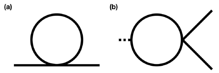
Figure 1: The diagrams that renormalize $\Phi_{2}$ at the first order of $\epsilon$. In the bulk the first diagram only shifts the mass of $\phi_{a}$, but at the boundary it makes a nontrivial contribution to the wave function renormalization.

The gauge invariant order parameter $\sum_{a}\phi_{a}^{2}$ we are interested in reduces to $\Phi_{2}=\sum_{a}\Phi^{2}_{1,a}$ at the boundary, and it has scaling dimension $[\Phi_{2}]=D$ at the mean field level. If the $Z_{2}$ gauge field is ignored, the correlation function of $\Phi_{1,a}$ at the boundary reads

$$\langle\Phi_{1,a}(\mathbf{x}_{1})\Phi^{\ast}_{1,a}(\mathbf{x}_{2})\rangle=\lim_{z_{1},z_{2}\rightarrow 0}\partial_{z_{1}}\partial_{z_{2}}G(\mathbf{x}_{1}-\mathbf{x}_{2},z_{1},z_{2}),$$ (8)

where $G(\mathbf{x}_{1}-\mathbf{x}_{2},z_{1},z_{2})$ is still given by the image method Eq. 6. If we assume that $G_{\mathrm{bulk}}$ takes the standard form at the Gaussian fixed point

$$\langle\phi_{a}(\mathbf{x}_{1},z_{1})\phi^{\ast}_{a}(\mathbf{x}_{2},z_{2})\rangle_{\mathrm{bulk}}$$ (9)

$$= \frac{1}{(|\mathbf{x}_{1}-\mathbf{x}_{2}|^{2}+(z_{1}-z_{2})^{2})^{\frac{D-2}{2}}},$$ (11)

the boundary correlation function of $\Phi_{1,a}$ at the mean field level reads

$$\langle\Phi_{1,a}(\mathbf{x}_{1})\Phi^{\ast}_{1,a}(\mathbf{x}_{2})\rangle=\frac{2(D-2)}{|\mathbf{x}_{1}-\mathbf{x}_{2}|^{D}}.$$ (12)

At the Gaussian fixed point, the correlation function of $\Phi_{2}$ can be derived using the Wick theorem:

$$\langle\Phi_{2}(\mathbf{x}_{1})\Phi^{\ast}_{2}(\mathbf{x}_{2})\rangle = \sum_{a}\langle\Phi_{1,a}(\mathbf{x}_{1})\Phi^{\ast}_{1,a}(\mathbf{x}_{2})\rangle^{2}$$ (13)

$$\sim \frac{1}{|\mathbf{x}_{1}-\mathbf{x}_{2}|^{2D}}.$$ (15)

The scaling dimension of $\Phi_{2}$ will acquire further correction from interaction, which can be computed through the $\epsilon=(4-D)$ expansion. Interestingly, at the leading $\epsilon$ order, $[\Phi_{2}]$ will receive corrections from both wave function renormalization and vertex corrections:

$$[\Phi_{2}]=D+2\delta_{wf}+\delta_{v}.$$ (16)

The wave function renormalization $\delta_{wf}$ can be extracted from the previously calculated $\epsilon-$expansion of the anomalous dimension at the boundary of the Wilson-Fisher fixed points, $i.e.$

$$[\Phi_{1,a}]=\frac{D}{2}+\delta_{wf}=\frac{D}{2}-\frac{N+1}{2(N+4)}\epsilon.$$ (17)

In contrast, in the bulk renormalization group (RG) analysis of the Wilson-Fisher fixed point, the wave function renormalization only appears at the second and higher order of $\epsilon$ expansion.

The vertex correction is most conveniently computed using the standard real-space RG, since now the momentum along the $\hat{z}$ direction is no longer conserved. We will use the following operator-product-expansion (OPE) between $\Phi_{2}(\mathbf{x},0)$ and the interaction term in Eq. 1 (Fig. 1$b$), where $\Phi_{2}(\mathbf{x},0)$ is defined as $\Phi_{2}(\mathbf{x},0)=\lim_{z\rightarrow 0}\left(\partial_{z}\phi(\mathbf{x},z)\right)^{2}$:

$$\Phi_{2}(\mathbf{x},0)g\left(\sum_{a}\phi^{\ast}_{a}(\mathbf{x}^{\prime},z^{\prime})\phi_{a}(\mathbf{x}^{\prime},z^{\prime})\right)^{2}$$ (18)

$$= 2g\lim_{z\rightarrow 0}(\partial_{z}G(\mathbf{x}-\mathbf{x}^{\prime},z,z^{\prime}))^{2}\sum_{a}\phi^{2}_{a}(\mathbf{x}^{\prime},z^{\prime})$$ (20)

$$\sim \frac{32z^{\prime 4}g}{\left((\mathbf{x}-\mathbf{x}^{\prime})^{2}+z^{\prime 2}\right)^{4}}\lim_{z\rightarrow 0}\left(\partial_{z}\phi(\mathbf{x},z)\right)^{2}.$$ (22)

Notice that like all the $4-\epsilon$ expansions, the OPE and loop integrals were performed by assuming the bulk system is in a four dimensional space-time. Under rescaling $\mathbf{x}\rightarrow\mathbf{x}/b$, through the vertex correction the operator $\Phi_{2}$ will acquire a correction

$$\delta\Phi_{2} = -\Phi_{2}\int^{a}_{a/b}4\pi r^{2}dr\int_{0}^{+\infty}dz^{\prime}\ \frac{32z^{\prime 4}g}{\left(r^{2}+z^{\prime 2}\right)^{4}}$$ (23)

$$= -4g\pi^{2}\left(\ln b\right)\Phi_{2}.$$ (25)

The integral of $z^{\prime}$ is within the upper semi-infinite plane $z^{\prime}>0$.

Using epsilon expansion, $g$ will flow from the noninteracting Gaussian fixed point to an interacting fixed point $g_{\ast}=\epsilon/(4(N+4)\pi^{2})$. Plugging the fixed point value of $g$ into Eq. 25, we obtain the vertex correction

$$\delta_{v}=\frac{\epsilon}{N+4}.$$ (26)

The wave function renormalization $\delta_{wf}$ can be reproduced in the same way through OPE (Fig. 1$a$). Eventually the scaling dimension of the gauge invariant order parameter $\Phi_{2}$ at the boundary is

$$[\Phi_{2}]=D-\frac{N\epsilon}{N+4}.$$ (27)

We have also confirmed these calculations through direct computation of the correlation function of $\Phi_{2}$ near the boundary (with diagrams in Fig. 2).

As we discussed before, the case with $N=1$ can be realized as the transition between a $Z_{2}$ topological order and a superconductor. If the system is probed from the boundary, in the ordered phase but close to the critical point, the superconductor order parameter should scale with the tuning parameter $r$ as

$$\Delta\sim|r|^{[\Phi_{2}]\nu}\sim|r|^{1.87},$$ (28)

and we have taken $\nu\sim 2/3$ for the XY^∗ fixed point Calabrese et al. (2003).

For $N=2$, the $\Phi_{2}$ operator is one component of the noncollinear spin order of a ${\rm SU}(2)$ spin system, which scales as

$$\langle\vec{S}\rangle\sim\Phi_{2}\sim|r|^{[\Phi_{2}]\nu}=|r|^{1.97}$$ (29)

Again, we have taken $\nu=0.74$ for the $\mathrm{O}(4)^{\ast}$ fixed point Calabrese et al. (2003). As a comparison, in the $2d$ bulk $\Phi_{2}$ should scale with $r$ as $\Phi_{2}\sim|r|^{0.82}(N=1)$ and $\Phi_{2}\sim|r|^{0.87}(N=2)$ respectively, which is significantly different from the boundary scaling.

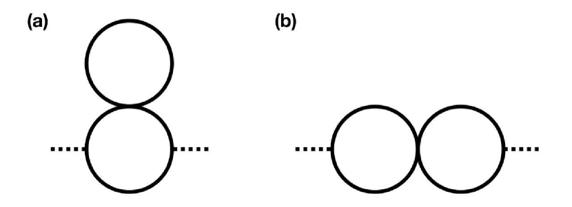
Figure 2: The renormalization of operator $\Phi_{2}$ at the leading order of $\epsilon$ can also be computed directly using the correlation functions in this figure.

When $N=1$, the action Eq. 1 may or may not allow an extra chemical potential term $\mu\phi^{\ast}\partial_{\tau}\phi$, depending on whether the system has a (emergent) particle-hole symmetry $\phi\rightarrow\phi^{\ast}$ or not. With nonzero $\mu$ the system has the same scaling as a mean field transition (with logarithmic corrections) as the total space-time dimension is effectively $D=2+d=4$, and $g$ is marginally irrelevant. In this case the scaling dimension of the Cooper pair at the boundary becomes $[\Phi^{2}]_{\mu\neq 0}=D=4$, and $\nu=1/2$ as in the mean field transition.

The boundary scaling is valid as long as we consider correlation function $G(\mathbf{x}_{1}-\mathbf{x}_{2},z_{1},z_{2})$ with $|\mathbf{x}_{1}-\mathbf{x}_{2}|\gg z_{1},z_{2}$. Right at the boundary of a $2d$ $Z_{2}$ topological order, the gauge field is confined, due to the condensation of the $m-$anyons of the $Z_{2}$ topological order at the boundary (the boundary of a $Z_{2}$ topological order can also have $e-$anyon condensate, but since in our case the $e-$anyons carry nontrivial symmetry transformations, we assume our boundary always has $m-$anyon condensate). Near the boundary, the system still has a finite confinement length $\xi(z)$ as a function of $z$, $i.e.$ the distance from the boundary, due to the “proximity effect” of the $m-$condensation at the boundary. In order to guarantee that we can approximately assume a deconfined $Z_{2}$ gauge field near the boundary, we need $\xi(z)\gg z$.

The most convenient way to estimate the confinement length $\xi(z)$ close to the boundary, is to evaluate the energy cost of two gauge charged particles separated with distance $x$ near the boundary. This energy cost can be estimated in the “dual” Hamiltonian of a $Z_{2}$ gauge theory, which is a $(2+1)d$ quantum Ising model: $H_{\mathrm{dual}}=\sum_{\bar{j}}-h\tau^{x}_{\bar{j}}-\sum_{\mu=x,y}J_{\bar{j},\mu}\tau^{z}_{\bar{j}}\tau^{z}_{\bar{j}+\mu}$, where $\tau^{x}_{\bar{j}}$, $\tau^{z}_{\bar{j}}$ are a pair of Pauli operators defined on the dual lattice sites $\bar{j}$. The dual Ising operator $\tau^{z}_{\bar{j}}$ is a creation/annihilation operator of the $Z_{2}$ gauge flux. A confined (and deconfined) phase of the $Z_{2}$ gauge field corresponds to the ordered (and disordered) phase of the dual quantum Ising model with nonzero (and zero) expectation value $\langle\tau^{z}\rangle$ Fradkin and Susskind (1978). If there is a pair of static $e-$particles with $Z_{2}$ gauge charges separated with distance $x$, this system is dual to a frustrated Ising model with $J_{\bar{j},\mu}=-J$ on the links along the branch-cut that connects the two particles, while $J_{\bar{j},\mu}=+J$ everywhere else. The energy cost of the two separated static particles corresponds to the energy difference between this frustrated Ising model nonuniform $J_{\bar{j},\mu}$, and the case with uniform $J_{\bar{j},\mu}$. Then if $\tau^{z}_{\bar{j}}$ has a nonzero expectation value $\langle\tau^{z}\rangle$, the pair of $Z_{2}-$gauge charges will approximately cost energy $E\sim J\langle\tau^{z}\rangle^{2}x$, $i.e.$ the system is in a confined phase with a linear confining potential between the two $Z_{2}$ gauge charges, and the confinement length is roughly $\xi\sim 1/(J\langle\tau^{z}\rangle^{2})$. In our system with a boundary at $z=0$, although $\langle\tau^{z}\rangle$ is nonzero at the boundary, its expectation value decays exponentially with $z$ because the $Z_{2}$ gauge field is in a deconfined phase deep in the bulk with $\langle\tau^{z}\rangle=0$. Hence the confinement length $\xi(z)$ also increases with $z$ exponentially, and we can safely assume that the $Z_{2}$ gauge field is still approximately deconfined near the boundary.

.3 Continuous Metal-Insulator transition

Another unconventional quantum phase transition that can happen in $2d$ systems is the continuous metal-insulator transition, where the insulator is a ${\rm U}(1)$ liquid phase with a fermi surface of the fermionic parton $f_{j,\alpha}$. Both $f_{j,\alpha}$ and $b_{j}$ are coupled to an emergent ${\rm U}(1)$ gauge field, which is presumably deconfined in the $2d$ bulk due to the existence of the Fermi surface and finite density of states of the matter fields. The critical behavior of this transition in the bulk was studied in Ref. Senthil, 2008, and it is again described by the condensation of $b_{j}$, but in this case $b_{j}$ is coupled to an dynamic ${\rm U}(1)$ gauge field $a_{\mu}$.

Although there is a gapless gauge field $a_{\mu}$ in the bulk, the gauge field dynamics is over-damped by the fermi surface of $f_{\alpha}$ through a term $\mathcal{S}_{\mathrm{damp}}\sim\frac{1}{e^{2}}\sum_{\omega,\vec{q}}|a^{t}_{\omega,q}|^{2}\frac{|\omega|}{|q|}$ based on the standard Hertz-Millis formalism Hertz (1976); Millis (1993), where $a^{t}$ is the transverse mode of the gauge field. A simple power-counting would suggest that the gauge coupling $e^{2}$ becomes irrelevant at the transition where $b_{j}$ condenses, for both $\mu=0$ and $\mu\neq 0$. Hence the universality class of this transition does not receive relevant infrared corrections from the gauge field. Moreover, the direct density-density interaction between the bosonic and fermionic partons also does not lead to relevant effects Senthil (2008). Hence the metal-insulator transition can still be described by Eq. 1. The quasiparticle residue is proportional to $|\langle b\rangle|$, and the electron Green’s function is proportional to $|\langle b\rangle|^{2}$. Hence if one probes from the boundary, the local density of states of electrons at low energy, which is proportional to the electron Green’s function, scales with the tuning parameter $r$ as

$$\rho\sim|\langle\Phi_{1}\rangle^{2}|\sim|r|^{2[\Phi_{1}]\nu}.$$ (30)

For $\mu=0$, $[\Phi_{1}]$ is calculated in Eq. 17, and $\nu\sim 2/3$; for $\mu\neq 0$, $[\Phi_{1}]=2$ and $\nu=1/2$.

Again we need to address the question of confinement length near the boundary, and demonstrate that $\xi(z)\gg z$. A pure ${\rm U}(1)$ gauge field in $(2+1)d$ is dual to a scalar boson $\varphi\sim\exp(\mathrm{i}\theta)$ which physically is the Dirac monopole operator, and the confined phase of a ${\rm U}(1)$ gauge field corresponds to a phase with a pinned nonzero expectation value of $\varphi$. A ${\rm U}(1)$ gauged particle becomes a vortex of $\theta$ in the dual formalism, and in a deconfined phase a vortex costs logarithmically divergent energy; but if $\varphi$ has a pinned nonzero expectation value, a vortex will cost linearly diverging energy and hence confined. Now suppose we consider a pair of gauge charged particles separated at distance $x$, the energy cost will be roughly $x\langle\varphi\rangle^{2}$. Hence we need to evaluate $\langle\varphi(z)\rangle$ as a function of $z$ away from the boundary, assuming a nonzero expectation value of $\varphi$ at the boundary $\varphi_{0}=\langle\varphi(z=0)\rangle$. $\langle\varphi(z)\rangle$ can be inferred from the correlation function $\langle\varphi(z)\rangle\sim\langle\varphi(z)\varphi(0)^{\ast}\rangle\sim\exp(\langle\theta(z)\theta(0)\rangle)$.

A $(2+1)d$ pure ${\rm U}(1)$ gauge field without the matter field is dual to a scalar boson model with an ordinary action $\mathcal{S}\sim\int d^{2}xd\tau\rho_{s}(\partial_{\mu}\theta)^{2}$, then $\theta$ has a positive scaling dimension $[\theta]=1/2$. The correlation function of $\theta$ reads $\langle\theta(r)\theta(0)\rangle\sim 1/r$, which makes the correlation function of the monopole operator saturates to a nonzero value as $r\rightarrow\infty$. Hence a positive scaling dimension of $\theta$ in the dual action renders the confinement of the compact gauge field in $(2+1)d$. If $\theta$ has a negative scaling dimension in its (dual) action, the correlation function of $\varphi$ will decay exponentially. Then the confinement length $\xi(z)\sim 1/\langle\varphi(z)\rangle^{2}\sim 1/\langle\varphi(z)\varphi(0)^{\ast}\rangle^{2}$ will grow exponentially with $z$ in the bulk away from the boundary. And since $\xi(z)\gg z$, the boundary scaling behavior calculated in this work can be applied under the assumption that the gauge field is sufficiently deconfined near the boundary since the confinement length is long enough in the vicinity of the boundary.

Now we need to derive the dual action for $\theta$ more carefully. Schematically the action for the transverse gauge field is

$$\mathcal{S}=\sum_{\omega,\vec{q}}\frac{1}{2}\left(\frac{1}{e^{2}}\frac{|\omega|}{q}+c^{2}q^{2}\right)|a^{t}|^{2}.$$ (31)

The canonical conjugate field of $\vec{a}$, $i.e.$ the electric field of the gauge field is defined as $\vec{E}=\delta\mathcal{L}/\delta\dot{\vec{a}}$, hence $\vec{E}_{\omega,\vec{q}}\sim\vec{a}_{\omega,\vec{q}}/(e^{2}q)$, hence the action can also be written as

$$\mathcal{S}=\sum_{\omega,\vec{q}}\frac{e^{2}}{2}|\omega||\vec{q}||\vec{E}_{\omega,\vec{q}}|^{2}+\frac{c^{2}}{2}q^{2}|a^{t}_{\omega,\vec{q}}|^{2}.$$ (32)

Then we can use the standard duality transformation that preserves the commutation relation between the canonical conjugate variables $\vec{E}$ and $\vec{A}$: $\vec{E}=\vec{\nabla}\theta$, $\vec{\nabla}\times\vec{a}=n$, where $n$ is the flux density, or the particle density conjugate to $\theta$. Eventually the dual action reads

$$\mathcal{S}_{d}=\sum_{\omega,\vec{q}}\frac{1}{2}\left(e^{2}|\omega|q^{3}+\frac{1}{c^{2}}\omega^{2}\right)|\theta_{\omega,\vec{q}}|^{2}.$$ (33)

Indeed, $\theta(\mathbf{x},\tau)$ has a negative scaling dimension in this dual action, which is consistent with our expectation that $\langle\varphi(z)\rangle$ decays exponentially in the bulk, hence the gauge field is still approximately deconfined in the vicinity of the boundary.

.4 Discussion

In this work we computed the boundary universal scaling behaviors of a class of deconfined quantum phase transitions, which is relevant to future realization of these exotic transitions in experimental systems. From the perspective of the pure Laudau’s paradigm, the cases we study correspond to the “ordinary transitions” of boundary CFT Cardy (1996), meaning the bulk will enter an ordered phase before the boundary, which we believe is the most natural case in real systems. Measurement of the scaling laws we calculated depends on the specific realization of the theory Eq. 1. For example, if the $N=1$ theory is realized (as we proposed in this work) as the transition between the $Z_{2}$ spin liquid to superconductor, the amplitude of the Cooper pair at the boundary predicted in our calculation can be measured through the Josephson effect by building a junction between the boundary of the system and another ordinary bulk superconductor, as the Josephson current is proportional to the amplitude of the superconductor order parameter near the boundary. The Josephson current should follow the same scaling law as Eq. 28.

The studies in this work can be naturally generalized to higher dimensions. If there is a deconfined QCP between the $Z_{2}$ topological order and an ordered phase in the $(3+1)d$ bulk, at its $(2+1)d$ boundary the gauge invariant order parameter $\Phi_{2}$ has precise scaling dimension $[\Phi_{2}]=4$, since in the bulk this transition is described by a mean field theory and received no extra corrections.

The direct transition between the Néel and valance bond solid (VBS) order is another type of deconfined QCP that has attracted a great deal of attentions. The boundary effect of this deconfined QCP is more complex than the situations we have considered because the boundary breaks the lattice symmetry, hence the boundary condition would couple to the VBS order parameter. Another interesting scenario worth studying is the boundary scaling of a bulk transition between a symmetry protected topological (SPT) states and an ordered phase which spontaneously breaks part of the defining symmetries of the SPT phase. Although the bulk transition should belong to the same universality class as the ordinary Ginzburg-Landau transition, its boundary is expected to be very different due to the existence of symmetry protected nontrivial boundary states even in the SPT phase. Efforts have been made along this direction including numerical simulation Zhang and Wang (2017) and construction of exactly soluble models Scaffidi et al. (2017). We will leave these subjects to future studies.

This work is supported by NSF Grant No. DMR-1920434, the David and Lucile Packard Foundation, and the Simons Foundation.

References

- WEN (1992) X.-G. WEN, International Journal of Modern Physics B 06, 1711 (1992), eprint https://doi.org/10.1142/S0217979292000840, URL https://doi.org/10.1142/S0217979292000840.
- WEN (1991) X.-G. WEN, International Journal of Modern Physics B 05, 1641 (1991), eprint https://doi.org/10.1142/S0217979291001541, URL https://doi.org/10.1142/S0217979291001541.
- Chen et al. (2013) X. Chen, Z.-C. Gu, Z.-X. Liu, and X.-G. Wen, Phys. Rev. B 87, 155114 (2013).
- Chen et al. (2012) X. Chen, Z.-C. Gu, Z.-X. Liu, and X.-G. Wen, Science 338, 1604 (2012).
- Senthil et al. (2004a) T. Senthil, A. Vishwanath, L. Balents, S. Sachdev, and M. P. A. Fisher, Science 303, 1490 (2004a).
- Senthil et al. (2004b) T. Senthil, L. Balents, S. Sachdev, A. Vishwanath, and M. P. A. Fisher, Phys. Rev. B 70, 144407 (2004b).
- Isakov et al. (2011) S. V. Isakov, M. B. Hastings, and R. G. Melko, Nature Physics 7, 772 (2011).
- Isakov et al. (2012) S. V. Isakov, M. B. Hastings, and R. G. Melko, Science 335, 193 (2012).
- Chubukov et al. (1994) A. V. Chubukov, S. Sachdev, and T. Senthil, Nuclear Physics B 426, 601 (1994), ISSN 0550-3213, URL http://www.sciencedirect.com/science/article/pii/055032139490%023X.
- XU (2012) C. XU, International Journal of Modern Physics B 26, 1230007 (2012), eprint https://doi.org/10.1142/S0217979212300071, URL https://doi.org/10.1142/S0217979212300071.
- Sandvik (2007) A. W. Sandvik, Phys. Rev. Lett. 98, 227202 (2007), URL https://link.aps.org/doi/10.1103/PhysRevLett.98.227202.
- Shao et al. (2016) H. Shao, W. Guo, and A. W. Sandvik, Science 352, 213 (2016), ISSN 0036-8075, eprint https://science.sciencemag.org/content/352/6282/213.full.pdf, URL https://science.sciencemag.org/content/352/6282/213.
- Melko and Kaul (2008) R. G. Melko and R. K. Kaul, Phys. Rev. Lett. 100, 017203 (2008), URL https://link.aps.org/doi/10.1103/PhysRevLett.100.017203.
- Qin et al. (2017) Y. Q. Qin, Y.-Y. He, Y.-Z. You, Z.-Y. Lu, A. Sen, A. W. Sandvik, C. Xu, and Z. Y. Meng, Phys. Rev. X 7, 031052 (2017), URL https://link.aps.org/doi/10.1103/PhysRevX.7.031052.
- Geim and Grigorieva (2013) A. K. Geim and I. V. Grigorieva, Nature 499, 419 (2013).
- Cardy (1996) J. Cardy, Scaling and Renormalization in Statistical Physics (Cambridge Lecture Notes in Physics, 1996).
- Dietrich and Diehl (1983) S. Dietrich and H. W. Diehl, Zeitschrift für Physik B Condensed Matter 51, 343 (1983), ISSN 1431-584X, URL https://doi.org/10.1007/BF01319217.
- Diehl and Dietrich (1981) H. W. Diehl and S. Dietrich, Zeitschrift für Physik B Condensed Matter 42, 65 (1981), ISSN 1431-584X, URL https://doi.org/10.1007/BF01298293.
- Reeve and Guttmann (1981) J. Reeve and A. J. Guttmann, Journal of Physics A: Mathematical and General 14, 3357 (1981), URL https://doi.org/10.1088%2F0305-4470%2F14%2F12%2F028.
- Cardy (1984) J. L. Cardy, Nuclear Physics B 240, 514 (1984), ISSN 0550-3213, URL http://www.sciencedirect.com/science/article/pii/055032138490%2414.
- Read and Sachdev (1991) N. Read and S. Sachdev, Phys. Rev. Lett. 66, 1773 (1991), URL http://link.aps.org/doi/10.1103/PhysRevLett.66.1773.
- Sachdev and Read (1991) S. Sachdev and N. Read, International Journal of Modern Physics B 05, 219 (1991), eprint https://doi.org/10.1142/S0217979291000158, URL https://doi.org/10.1142/S0217979291000158.
- Wu et al. (2003) C. Wu, J.-p. Hu, and S.-c. Zhang, Phys. Rev. Lett. 91, 186402 (2003), URL https://link.aps.org/doi/10.1103/PhysRevLett.91.186402.
- Calabrese et al. (2003) P. Calabrese, A. Pelissetto, and E. Vicari, arXiv:cond-mat/0306273 (2003).
- Fradkin and Susskind (1978) E. Fradkin and L. Susskind, Phys. Rev. D 17, 2637 (1978), URL https://link.aps.org/doi/10.1103/PhysRevD.17.2637.
- Senthil (2008) T. Senthil, Phys. Rev. B 78, 045109 (2008), URL https://link.aps.org/doi/10.1103/PhysRevB.78.045109.
- Hertz (1976) J. A. Hertz, Phys. Rev. B 14, 1165 (1976), URL https://link.aps.org/doi/10.1103/PhysRevB.14.1165.
- Millis (1993) A. J. Millis, Phys. Rev. B 48, 7183 (1993), URL https://link.aps.org/doi/10.1103/PhysRevB.48.7183.
- Zhang and Wang (2017) L. Zhang and F. Wang, Phys. Rev. Lett. 118, 087201 (2017), URL https://link.aps.org/doi/10.1103/PhysRevLett.118.087201.
- Scaffidi et al. (2017) T. Scaffidi, D. E. Parker, and R. Vasseur, Phys. Rev. X 7, 041048 (2017), URL https://link.aps.org/doi/10.1103/PhysRevX.7.041048.