Variational phase recovering without phase unwrapping in phase-shifting interferometry

Abstract

We present a variational method for recovering the phase term from the information obtained from phase-shifting methods. First we introduce the new method based on a variational approach and then describe the numerical solution of the proposed cost function, which results in a simple algorithm. Numerical experiments with both synthetic and real fringe patterns shows the accuracy and simplicity of the resulting algorithm.

1 Introduction

The main goal of fringe analysis techniques is to recover accurately the modulated phase from one or several fringe patterns ^{20, 19}; such phase is related to some physical quantities like shape, deformation, refractive index, temperature, etc. The basic model for a fringe pattern is given by

$$I_{\mathbf{x}}=a_{\mathbf{x}}+b_{\mathbf{x}}\cos\left(\phi_{\mathbf{x}}\right),$$

where $\mathbf{x}=(x,y)$, $a_{\mathbf{x}}$ is the background illumination, $b_{\mathbf{x}}$ is the amplitude modulation, and $\phi_{\mathbf{x}}$ is the phase map to be recovered.

Among the methods for phase estimation is the phase-shifting method ^{3, 23}, which consists in acquiring several fringe patterns where the phase term is incremented between successive frames. Such fringe patterns are defined as

$$I_{\mathbf{x},k}=a_{\mathbf{x}}+b_{\mathbf{x}}\cos\left(\phi_{\mathbf{x}}+\alpha_{k}\right),\;k=1,\ldots,K,\;K\geq 3,$$

where $\alpha_{k}$ is the phase step and $K$ is the number of fringe patterns used. For every $\alpha_{k}$, the fringe pattern can be written as

$$I_{\mathbf{x},k}=a_{\mathbf{x}}+b_{\mathbf{x}}\cos\left(\phi_{\mathbf{x}}+\alpha_{k}\right)=I^{0}_{\mathbf{x}}+I^{c}_{\mathbf{x}}\cos\left(\alpha_{k}\right)-I^{s}_{\mathbf{x}}\sin\left(\alpha_{k}\right)$$ (1)

where

$$I^{0}_{\mathbf{x}} =a_{\mathbf{x}},$$

$$I^{c}_{\mathbf{x}} =b_{\mathbf{x}}\cos\left(\phi_{\mathbf{x}}\right),$$

$$I^{s}_{\mathbf{x}} =b_{\mathbf{x}}\sin\left(\phi_{\mathbf{x}}\right).$$

The funtions $I^{0}_{\mathbf{x}},I^{c}_{\mathbf{x}},I^{s}_{\mathbf{x}}$ can be estimated with different phase-shifting techniques ^{26, 27, 30, 31, 32}. Using these coefficients, the wrapped phase term can be computed by ¹⁴

$$\hat{\phi}_{\mathbf{x}}=\mathtt{atan2}\left[I^{s}_{\mathbf{x}},I^{c}_{\mathbf{x}}\right]=\phi_{\mathbf{x}}\,\bmod{2\pi}.$$ (2)

Then the phase term $\phi_{\mathbf{x}}$ is estimated by a process named phase unwrapping ⁵, which is usually computationally intensive and susceptible to noise. To avoid these drawbacks, several approaches have been developed to estimate the phase without the need of the unwrapping process ^{22, 12, 11, 33}.

A different approach is found in reference 17, where the information obtained from the phase-shifting method, given in Eq. (1), is used to estimate the phase term $\phi_{\mathbf{x}}$ from the information of $I^{c}_{\mathbf{x}}$ and $I^{s}_{\mathbf{x}},$ and the partial derivatives of these two functions, respectively. This approach consists in computing the gradient field as follows:

$$\Phi_{\mathbf{x}} =\left(\Phi_{\mathbf{x}}^{1},\;\Phi_{\mathbf{x}}^{2}\right)=\left(\frac{\partial\phi_{\mathbf{x}}}{\partial x},\;\frac{\partial\phi_{\mathbf{x}}}{\partial y}\right)$$ (3)

$$=\left(\frac{\frac{\partial I^{s}_{\mathbf{x}}}{\partial x}\,I^{c}_{\mathbf{x}}\;-\;I^{s}_{\mathbf{x}}\,\frac{\partial I^{c}_{\mathbf{x}}}{\partial x}}{\left(I^{c}_{\mathbf{x}}\right)^{2}+\left(I^{s}_{\mathbf{x}}\right)^{2}},\;\frac{\frac{\partial I^{s}_{\mathbf{x}}}{\partial y}\,I^{c}_{\mathbf{x}}\;-\;I^{s}_{\mathbf{x}}\,\frac{\partial I^{c}_{\mathbf{x}}}{\partial y}}{\left(I^{c}_{\mathbf{x}}\right)^{2}+\left(I^{s}_{\mathbf{x}}\right)^{2}}\right).$$

From the gradient field $\Phi_{\mathbf{x}}$, the phase term $\phi_{\mathbf{x}}$ is estimated by using line integrals ¹⁷. In this way, the non-linearity of the arctangent function, Eq. (2), is avoided. This approach has been successfully used on the demodulation of fringe patterns obtained from phase-shifting methods ^{27, 28}. However, the line integrals approach fails with moderate levels of noise and/or aliasing in the input fringe patterns, in the same way the Itoh’s method does ⁵.

In this work we present a method for recovering the phase term $\phi_{\mathbf{x}}$ from the information obtained from phase-shifting methods; that is, using only the fringe patterns $I^{c}_{\mathbf{x}}$ and $I^{s}_{\mathbf{x}}$, avoiding the use of the nonlinear arctangent function. First we introduce the new method based on a variational approach. Then we describe the numerical solution of the proposed cost function, which results in a simple algorithm. The performance of the proposed method is evaluated by numerical experiments with both synthetic and real data. A comparison against two well-known least-square based unwrapping methods is also presented. Finally we discuss our results and present some concluding remarks.

2 A new variational model for the recovery of the phase from phase-shifting method

2.1 Variational Formulation

Variational techniques have been successfully used in fringe pattern processing. In the literature it is possible to find several works about fringe-pattern filtering ^{34, 35, 13}, demodulation ¹¹, unwrapping ¹⁰ and gradient-field estimation of a wrapped-phase for unwrapping processing ⁷.

In this work, we propose to estimate the phase map $\phi_{\mathbf{x}}$ as the solution of the minimization problem defined by

$$\underset{\phi}{\min}\;E(\phi_{\mathbf{x}}),$$ (4)

where

$$E(\phi_{\mathbf{x}}) =\frac{1}{2}\int_{\Omega}\left|\nabla\phi_{\mathbf{x}}-\Phi_{\mathbf{x}}\right|^{2}d\mathbf{x}+\frac{1}{2}\int_{\Omega}\left(b_{\mathbf{x}}\cos\phi_{\mathbf{x}}-I^{c}_{\mathbf{x}}\right)^{2}d\mathbf{x}$$

$$+\frac{1}{2}\int_{\Omega}\left(b_{\mathbf{x}}\sin\phi_{\mathbf{x}}-I^{s}_{\mathbf{x}}\right)^{2}d\mathbf{x}+\frac{\lambda}{2}\int_{\Omega}\left|\nabla\phi_{\mathbf{x}}\right|^{2}d\mathbf{x}$$

and $I^{s}_{\mathbf{x}},$ $I^{c}_{\mathbf{x}}$ are the input fringe patterns obtained from the phase-shifting method, given in Eq. (1); the term $b_{\mathbf{x}}$ is estimated from these fringe patterns in the following way

$$b_{\mathbf{x}}=\sqrt{\left(I^{s}_{\mathbf{x}}\right)^{2}+\left(I^{c}_{\mathbf{x}}\right)^{2}}.$$

The term $\Phi_{\mathbf{x}}$ is the gradient field estimated from the input fringe patterns described in Eq. (3), $\Omega\subset\mathbb{R}^{2}$ denotes the continuous signal domain, and $\lambda>0$ is a Lagrange multiplier.

The motivation to our proposed model is two fold. First, we note that the first term in Eq.(4) penalizes the differences between the known and possibly noisy gradient phase field and the recovered gradient phase field, and this term can be seen as an equivalent expression of the least-square approach to the phase unwrapping technique described in reference 5. Also, by the action of the last term, the recovered phase field will be smoothed and the problem made well-posed. By just using these two terms, there will be many possible solutions since the gradient field of more than one phase surface will be a feasible solution. In order to avoid this problem, we inserted the second and third terms in Eq.(4), to enforce the solution to be close to the input information, see Eqs. (1) and (3). In that sense, our model is more robust than similar models used in unwrapping processes that lack a way to constrain the solution to the expected scale and shape.

To obtain the solution of the problem expressed in Eq.(4), the first order optimality condition or Euler-Lagrange equation has to be derived. In the formal derivation we assume that the function $\phi_{\mathbf{x}}$ is smooth enough such that gradients are well defined and the variation $\delta\phi_{\mathbf{x}}$ has compact support over $\Omega$ so that we can use the divergence theorem to get rid of the boundary term.

To simplify notation, write $\left\langle f\right\rangle=\int_{\Omega}f\,d\mathbf{x}$ or $\left\langle f\right\rangle_{\partial}=\int_{\partial\Omega}f\,d\mathbf{x}$ depending on whether the integral is evaluated on the domain $\Omega$ or its boundary $\partial\Omega$. Then the first variation is derived as

$$\delta E(\phi_{\mathbf{x}}) =\frac{1}{2}\left\langle\delta\big{|}\nabla\phi_{\mathbf{x}}-\Phi_{\mathbf{x}}\big{|}^{2}\right\rangle+\frac{1}{2}\left\langle\delta\big{(}b_{\mathbf{x}}\cos\phi_{\mathbf{x}}-I^{c}_{\mathbf{x}}\big{)}^{2}\right\rangle$$ (5)

$$+\frac{1}{2}\left\langle\delta\big{(}b_{\mathbf{x}}\sin\phi_{\mathbf{x}}-I^{s}_{\mathbf{x}}\big{)}^{2}\right\rangle+\frac{\lambda}{2}\left\langle\delta\big{|}\nabla\phi_{\mathbf{x}}\big{|}^{2}\right\rangle$$

$$=\frac{1}{2}\left\langle 2\big{(}\nabla\phi_{\mathbf{x}}-\Phi_{\mathbf{x}}\big{)}\cdot\delta\nabla\phi_{\mathbf{x}}\right\rangle+\frac{1}{2}\left\langle 2\big{(}b_{\mathbf{x}}\cos\phi_{\mathbf{x}}-I^{c}_{\mathbf{x}}\big{)}\cdot\delta\left(b_{\mathbf{x}}\cos\phi_{\mathbf{x}}\right)\right\rangle$$

$$+\frac{1}{2}\left\langle 2\big{(}b_{\mathbf{x}}\sin\phi_{\mathbf{x}}-I^{s}_{\mathbf{x}}\big{)}\cdot\delta\left(b_{\mathbf{x}}\sin\phi_{\mathbf{x}}\right)\right\rangle+\frac{\lambda}{2}\left\langle 2\nabla\phi_{\mathbf{x}}\cdot\delta\nabla\phi_{\mathbf{x}}\right\rangle$$

$$=\left\langle\delta\phi_{\mathbf{x}}\big{(}\nabla\phi_{\mathbf{x}}-\Phi_{\mathbf{x}}\big{)}\cdot\mathbf{n}\right\rangle_{\partial}-\left\langle\nabla\cdotp\big{(}\nabla\phi_{\mathbf{x}}-\Phi_{\mathbf{x}}\big{)}\;\delta\phi_{\mathbf{x}}\right\rangle$$

$$+\left\langle\big{(}b_{\mathbf{x}}\cos\phi_{\mathbf{x}}-I^{c}_{\mathbf{x}}\big{)}\cdotp\big{(}-b_{\mathbf{x}}\sin\phi_{\mathbf{x}}\big{)}\;\delta\phi_{\mathbf{x}}\right\rangle$$

$$+\left\langle\big{(}b_{\mathbf{x}}\sin\phi_{\mathbf{x}}-I^{s}_{\mathbf{x}}\big{)}\cdotp\big{(}b_{\mathbf{x}}\cos\phi_{\mathbf{x}}\big{)}\;\delta\phi_{\mathbf{x}}\right\rangle$$

$$+\lambda\left\langle\delta\phi_{\mathbf{x}}\nabla\phi_{\mathbf{x}}\cdot\mathbf{n}\right\rangle_{\partial}-\lambda\left\langle\big{(}\nabla\cdotp\nabla\phi_{\mathbf{x}}\big{)}\;\delta\phi_{\mathbf{x}}\right\rangle$$

where in the last line we have used the divergence theorem and $\mathbf{n}$ denotes the unit outer normal vector to the boundary. Finally, the variational derivative of $E(\phi_{\mathbf{x}})$ is given by

$$\frac{\partial E(\phi_{\mathbf{x}})}{\partial\phi_{\mathbf{x}}} =-\nabla\cdotp\big{(}\nabla\phi_{\mathbf{x}}-\Phi_{\mathbf{x}}\big{)}+\big{(}b_{\mathbf{x}}\cos\phi_{\mathbf{x}}-I^{c}_{\mathbf{x}}\big{)}\cdotp\big{(}-b_{\mathbf{x}}\sin\phi_{\mathbf{x}}\big{)}$$ (6)

$$+\big{(}b_{\mathbf{x}}\sin\phi_{\mathbf{x}}-I^{s}_{\mathbf{x}}\big{)}\cdotp\big{(}b_{\mathbf{x}}\cos\phi_{\mathbf{x}}\big{)}-\lambda\nabla\cdotp\nabla\phi_{\mathbf{x}}$$

$$=-\left(1+\lambda\right)\nabla\cdotp\nabla\phi_{\mathbf{x}}+\nabla\cdotp\Phi_{\mathbf{x}}+I^{c}_{\mathbf{x}}\cdotp\big{(}b_{\mathbf{x}}\sin\phi_{\mathbf{x}}\big{)}-I^{s}_{\mathbf{x}}\cdotp\big{(}b_{\mathbf{x}}\cos\phi_{\mathbf{x}}\big{)}=0$$

with boundary conditions

$$\big{(}\nabla\phi_{\mathbf{x}}-\Phi_{\mathbf{x}}\big{)}\cdot\mathbf{n} =0$$ (7)

$$\nabla\phi_{\mathbf{x}}\cdot\mathbf{n} =0$$

2.2 Numerical Solution

Let $\phi_{i,j}=\phi(x_{i},y_{j})$ to denote the value of a grid function $\phi$ at point $(x_{i},y_{j})$ defined on $\Omega=[a,b]\times[c,d]$ where the sampling points of the grid are

$$x_{i} =a+(i-1)h_{x}$$

$$y_{j} =c+(j-1)h_{y}$$

with $1\leq i\leq m,\;1\leq j\leq n,$ and $h_{x}=(b-a)/(m-1),h_{y}=(d-c)/(n-1)$.

To approximate the derivatives, we use central finite differences between ghost half-points as follows

$$\delta_{x}\phi_{i,j}=\frac{\phi_{i+1/2,j}-\phi_{i-1/2,j}}{h_{x}},\quad\text{and}\quad\delta_{y}\phi_{i,j}=\frac{\phi_{i,j+1/2}-\phi_{i,j-1/2}}{h_{y}}.$$

The divergence term in Eq. (6) is approximated as

$$\nabla\cdot V_{i,j}=\delta_{x}V^{1}_{i,j}+\delta_{y}V^{2}_{i,j},$$

where

$$V_{i,j} =(V^{1}_{i,j},V^{2}_{i,j})=\nabla\phi_{i,j}-\Phi_{i,j},$$

$$\nabla\phi_{i,j} =(\delta_{x}\phi_{i,j},\delta_{y}\phi_{i,j}).$$

The rest of the terms in the equation are approximated by straight forward evaluation at point $(x_{i},y_{j})$.

To implement the boundary condition on $\partial\Omega$, we assume without loss of generality that $\mathbf{n}=(\pm 1,0)$ and $\mathbf{n}=(0,\pm 1)$ in the $x-$ and $y-$direction, respectively. With this consideration, the first boundary condition is expressed as

$$\delta_{x}\phi_{m,j}-\Phi_{m,j}^{1} =0\quad\text{for}\quad\mathbf{n}=(1,0),$$ (8)

$$-\left(\delta_{x}\phi_{1,j}-\Phi_{1,j}^{1}\right) =0\quad\text{for}\quad\mathbf{n}=(-1,0),$$

$$\delta_{y}\phi_{i,n}-\Phi_{i,n}^{2} =0\quad\text{for}\quad\mathbf{n}=(0,1),$$

$$-\left(\delta_{y}\phi_{i,1}-\Phi_{i,1}^{2}\right) =0\quad\text{for}\quad\mathbf{n}=(0,-1).$$

Examples of numerical implementations of similar functionals can be found on references 21 and 4.

3 Numerical Experiments

To illustrate the performance of the proposed method, we carried out some numerical experiments using a Intel Core i7 @ 2.40 GHz laptop with Debian GNU/Linux 8 (jessie) 64–bit and 16 GB of memory. For both experiments, we solve Eq. (6) using a fast variant of Nesterov’s method, which is an improvement of the gradient descent method ^{8, 16}. In our experiments we found that the Nesterov’s method is approximately 58 times faster than the gradient descent method, as far as iterations is concerned. This method is given by

$$\beta^{k+1}_{\mathbf{x}} =\phi^{k}_{\mathbf{x}}-\tau\;\frac{\partial E(\phi_{\mathbf{x}})}{\partial\phi_{\mathbf{x}}},$$ (9)

$$t^{k+1} =\frac{1+\sqrt{1+4\left(t^{k}\right)^{2}}}{2},$$

$$\phi^{k+1}_{\mathbf{x}} =\beta^{k+1}_{\mathbf{x}}+\frac{t^{k}-1}{t^{k+1}}\left(\beta^{k+1}_{\mathbf{x}}-\beta^{k}_{\mathbf{x}}\right)+\frac{t^{k}}{t^{k+1}}\left(\beta^{k+1}_{\mathbf{x}}-\phi^{k}_{\mathbf{x}}\right),$$

where $\beta^{0}_{\mathbf{x}}=\phi^{0}_{\mathbf{x}},$ $t^{0}=1$, $k=0,1,2,\ldots,$ and $\tau$ is the step size of the gradient descent. We chose the step size $\tau$ using the algorithm proposed in reference 24, which estimates the Lipschitz constant of the functional.

We use as stopping criteria for our optimization algorithm the same terms used in reference 29 with $\delta_{1}=\delta_{2}=\delta_{3}=10^{-7}$ and $k_{max}=15000.$ For simplicity, we selected the regularization parameter $\lambda$ manually; however, well known methods can be used to obtain the best parameter for this task, such as those described in section 5.6 of reference 1. In addition, we use a normalized error $Q$ to compare the phase-map estimation; this error is defined as ¹⁸:

$$Q\left(\mu,\nu\right)=\frac{\|\mu-\nu\|_{2}}{\|\mu\|_{2}+\|\nu\|_{2}},$$ (10)

where $\mu$ and $\nu$ are the signals to be compared. The normalized error values vary between zero (for perfect agreement) and one (for perfect disagreement).

3.1 Phase estimation using synthetic fringe patterns

The first set of experiments was the estimation of a synthetic phase map defined as ²⁷:

$$\phi_{\mathbf{x}}^{a} =1.3-1.9x-1.3\left(1-6y^{2}-6x^{2}+6y^{4}+12x^{2}y^{2}+6x^{4}\right)$$ (11)

$$+3.415\left(5xy^{4}-10x^{3}y^{2}+x^{5}\right)$$

$$+0.43\left(3x-12xy^{2}-12x^{3}+10xy^{4}+20x^{3}y^{2}+10x^{5}\right)$$

$$+2.6\left(-4y^{3}+12x^{2}y+5y^{5}-10x^{2}y^{3}-15x^{4}\right),$$

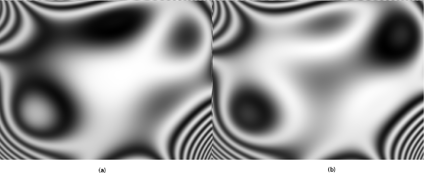
Figure 2: Fringe patterns generated with the phase map given in Eq. (11): (a) $I^{c}_{\mathbf{x}}$, (b) $I^{s}_{\mathbf{x}}$.

evaluated in a square domain $\Omega=\left\{(x,y)\,|\,-1\leq x,y\leq 1\right\}.$ Figure 1 shows the phase obtained from Eq. (11). Figure 2 shows the fringe patterns $I^{c}_{\mathbf{x}}$ and $I^{s}_{\mathbf{x}}$ (Eq. (1)) used in the estimation, with resolution of 640 $\times$ 480 pixels. A first experiment was the phase estimation using the fringe patterns shown in Figure 2, where $\lambda=1$ and the value for $\phi^{0}_{\mathbf{x}}$ was randomly generated. The estimated phase map is shown in Figure 3. The normalized error was $Q=0.0014$ and the time employed to obtain the solution was 106 seconds using 2342 iterations of the Nesterov’s method (Eq. (9)). Figure 4 shows the error obtained in this estimation.

A second estimation was made using fringe patterns with SNR = 12.5 db ⁶, shown in Figure 5. For this estimation, we use $\lambda=1.0$ and the initial value was randomly generated. The estimated phase map is shown in Figure 6. The normalized error was $Q=0.016$ and the time employed to obtain the solution was 123 seconds using 2819 iterations of the Nesterov’s method. Figure 7 shows the error obtained in this estimation. Table 1 presents a summary of the estimation performance of our proposed functional using the fringes patterns generated by Eq. (11) with different SNR.

A second experiment was the estimation of a synthetic phase map defined by the MATLAB peaks function², evaluated in a square domain
$\Omega=\left\{(x,y)\,|\,-2.3\leq x,y\leq 2.3\right\}.$ Figure 8 shows the wrapped phase generated by the peaks function, and Figure 9 shows the fringe patterns $I^{c}_{\mathbf{x}}$ and $I^{s}_{\mathbf{x}}$ (Eq. (1)) used in the estimation, with resolution of 640 $\times$ 480 pixels with SNR = 12.7 db. The resultant estimated phase map is shown in Figure 10 where the normalized error was $Q=0.014$ and the time employed to obtain the solution was 342 seconds using 7552 iterations of the Nesterov’s method. Figure 11 shows the error obtained in this estimation. Table 2 presents a summary of the estimation performance of our proposed functional using the fringes patterns generated by the MATLAB peaks function with different SNR.

3.2 Phase estimation using experimental fringe patterns

In this experiment we show the performance of the proposed method on the processing of experimental information with noise. This experiment consists of the phase estimation of a sequence of 5 fringe patterns obtained from a holographic interferometric experiment ⁹. Figure 12 shows the fringe patterns $I^{c}_{\mathbf{x}}$ and $I^{s}_{\mathbf{x}}$ (Eq. (1)) obtained from the phase-shifting method, with resolution of 640 $\times$ 480 pixels. The wrapped phase map obtained from these fringe patterns can be observed in Figure 13.

Due to the noisy phase-term, the strong variations in the modulation or the presence of phase-shift miscalibration ²⁵, the iterative process will be slow or even trapped on a local minimum. To improve the iterative process, we propose to use as initial value the phase term obtained from the method reported in reference 17. Figure 14 shows the estimated phase using $\lambda=1.5$; the normalized error was $Q=0.012$ and the time employed to obtain the solution was 87 seconds, including the time employed to estimate the initial value, using 1590 iterations of the Nesterov’s method.

To compare the performance of our proposal, we unwrap the phase map shown in Figure 13 with two unwrapping methods: a) the discrete version of Poisson equation (Eq. (5.31) of reference 5), and b) the method described in reference 15. For both cases, we used the Nesterov’s method as optimization technique. Figure 15 shows the estimated phase using reference 5, where the time employed to obtain the solution was 40 seconds, including the time employed to estimate the initial value, using 5205 iterations of the Nesterov’s method and the normalized error was $Q=0.015$. Figure 16 shows the estimated phase using reference 15 with $\lambda=1.2$, where the time employed to obtain the solution was 245 seconds, including the time employed to estimate the initial value, using 15000 iterations of the Nesterov’s method and the normalized error was $Q=0.241$.

4 Discussion of results and conclusions

As can be observed from the above experiments, the proposed method successfully estimates the unwrapped phase map from the information of the phase-shifting method methods; that is, the fringe patterns $I^{c}_{\mathbf{x}}$ and $I^{s}_{\mathbf{x}}$, without the use of the wrapped phase map. This method converges to an accurate solution given an arbitrary initial point, even for noisy fringe patterns. Due to the smoothing term included in the functional, it is possible to obtain a filtered phase map with the preservation of the dynamic range of the fringe patterns.

The numerical solution of Eq. (4) results on a very simple algorithm which estimate a filtered phase map in a short time, despite the optimization algorithm with poor convergence-rate used in experiments. In comparison with the methods described in reference 5 (Eq. (5.31) and reference 15, the proposed method shows a good performance on the estimation and the computational load employed to compute the phase map. To improve the convergence-rate, the proposed method can be easily implemented with a better computationally efficient techniques, including parallel approaches. This will be one aim of our future research.

Table 1: Estimation performance of Eq. (4) using fringes patterns generated with Eq. (11).

SNR (db)	iterations	Normalized error (Q)
$\inf$	2342	0.00142
39.97	2428	0.00335
27.98	2483	0.00980
21.08	2501	0.00867

Table 2: Estimation performance of Eq. (4) using fringes patterns generated with peaks function.

SNR (db)	iterations	Normalized error (Q)
$\inf$	5555	0.00072
40.26	5876	0.00366
28.22	6350	0.00603
21.22	6782	0.00823
14.44	7349	0.01076
12.72	7552	0.01427

Figures

Figure 1: Synthetic phase map given in Eq. (11).

Figure 3: Estimated phase map using fringe patterns shown in Fig. 2.

Figure 4: Absolute difference between the estimated phase map using fringe patterns shown in Fig. 2 and the synthetic phase map given in Eq. (11).

Figure 5: Noisy fringe patterns generated with the phase map given in Eq. (11): (a) $I^{c}_{\mathbf{x}}$, (b) $I^{s}_{\mathbf{x}}$.

Figure 6: Estimated phase map using fringe patterns shown in Fig. 5.

Figure 7: Absolute difference between the estimated phase map using fringe patterns shown in Fig. 5 and the synthetic phase map given in Eq. (11).

Figure 8: Synthetic phase map given by peaks function.

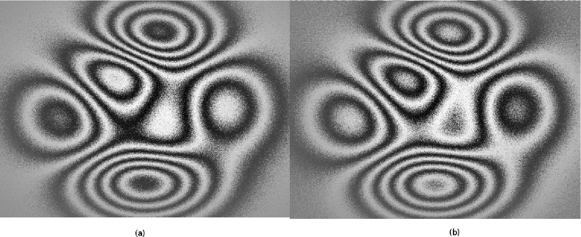
Figure 9: Noisy fringe patterns generated with the phase map given in Fig. 8: (a) $I^{c}_{\mathbf{x}}$, (b) $I^{s}_{\mathbf{x}}$.

Figure 10: Estimated phase map using fringe patterns shown in Fig. 9.

Figure 11: Absolute difference between the estimated phase map using fringe patterns shown in Fig. 9 and the synthetic phase map given by peaks function.

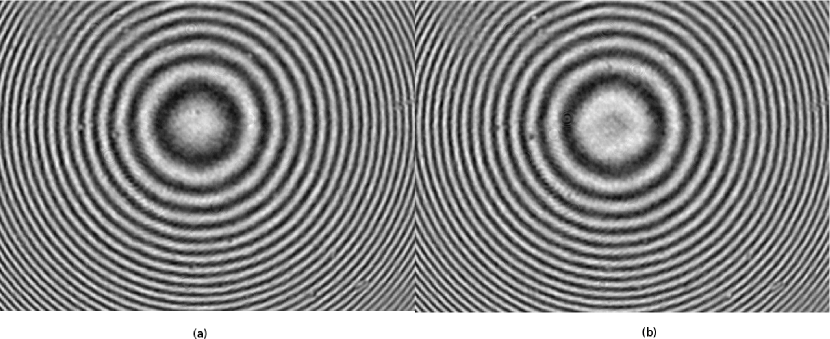
Figure 12: Experimental fringe patterns: (a) $I^{c}_{\mathbf{x}}$, (b) $I^{s}_{\mathbf{x}}$.

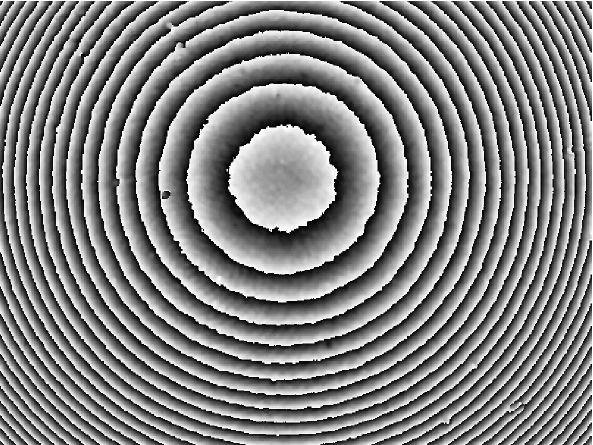
Figure 13: Wrapped phase map generated by the fringe patterns shown in Fig. 12

Figure 14: Estimated phase map using Eq. (4).

Figure 15: Estimated phase map using Eq. (5.31) of reference 5.

Figure 16: Estimated phase map using reference 15.

References

- 1 M. Bertero and P. Boccacci, Introduction to Inverse Problems in Imaging, Taylor & Francis, 1998.
- 2 T.A. Davis, MATLAB® Primer, 8th ed., CRC Press, 2014.
- 3 K.J. Gasvik., Optical metrology, 3rd ed., John Wiley & Sons, 2002.
- 4 P. Getreuer, Rudin-Osher-Fatemi Total Variation Denoising using Split Bregman, Image Processing On Line 2012 (2012), pp. 1–20. Available at http://dx.doi.org/10.5201/ipol.2012.g-tvd.
- 5 D.C. Ghiglia and M.D. Pritt, Two-Dimensional Phase Unwrapping: Theory, Algorithms, and Software, Wiley-Interscience, 1998.
- 6 R.C. Gonzalez and R.E. Woods, Digital Image Processing, 3rd ed., Pearson Prentice Hall, Upper Saddle River, NJ, 2008.
- 7 H.Y.H. Huang, L. Tian, Z. Zhang, Y. Liu, Z. Chen, and G. Barbastathis, Path-independent phase unwrapping using phase gradient and total-variation (TV) denoising, Optics Express 20 (2012), pp. 14075–14089. Available at http://dx.doi.org/10.1364/OE.20.014075.
- 8 D. Kim and J.A. Fessler, Optimized first-order methods for smooth convex minimization, Mathematical Programming 159 (2016), pp. 81–107. Available at http://dx.doi.org/10.1007/s10107-015-0949-3.
- 9 T. Kreis, Holographic Interferometry: Principles and Methods, Wiley-VCH, 1996.
- 10 C. Lacombe, P. Kornprobst, G. Aubert, and L. Blanc-Feraud, A variational approach to one dimensional Phase Unwrapping, in 16th International Conference on Pattern Recognition, 2002, Vol. 2. 2002, pp. 810–813. Available at http://dx.doi.org/10.1109/ICPR.2002.1048426.
- 11 R. Legarda-Saenz, C. Brito-Loeza, and A. Espinosa-Romero, Total variation regularization cost function for demodulating phase discontinuities, Applied Optics 53 (2014), p. 2297. Available at http://dx.doi.org/10.1364/AO.53.002297.
- 12 R. Legarda-Saenz, W. Osten, and W.P. Juptner, Improvement of the regularized phase tracking technique for the processing of nonnormalized fringe patterns, Applied Optics 41 (2002), pp. 5519–5526. Available at http://dx.doi.org/10.1364/AO.41.005519.
- 13 B. Li, C. Tang, G. Gao, M. Chen, S. Tang, and Z. Lei, General filtering method for electronic speckle pattern interferometry fringe images with various densities based on variational image decomposition, Applied Optics 56 (2017), p. 4843. Available at https://doi.org/10.1364/AO.56.004843.
- 14 D. Malacara, M. Servín, and Z. Malacara, Interferogram Analysis For Optical Testing, 2nd ed., CRC Press, 2005, Available at http://dx.doi.org/10.1201/9781420027273.fmatt.
- 15 J.L. Marroquin and M. Rivera, Quadratic regularization functionals for phase unwrapping, Journal of the Optical Society of America A 12 (1995), pp. 2393–2400. Available at http://dx.doi.org/10.1364/JOSAA.12.002393.
- 16 B. O’Donoghue and E. Candes, Adaptive Restart for Accelerated Gradient Schemes, Foundations of Computational Mathematics 15 (2015), pp. 715–732. Available at http://dx.doi.org/10.1007/s10208-013-9150-3.
- 17 G. Paez and M. Strojnik, Phase-shifted interferometry without phase unwrapping: reconstruction of a decentered wave front, Journal of the Optical Society of America A 16 (1999), p. 475. Available at https://doi.org/10.1364/JOSAA.16.000475.
- 18 M. Perlin and M.D. Bustamante, A robust quantitative comparison criterion of two signals based on the Sobolev norm of their difference, Journal of Engineering Mathematics 101 (2016), pp. 115–124. Available at http://dx.doi.org/10.1007/s10665-016-9849-7.
- 19 G. Rajshekhar and P. Rastogi, Fringe analysis : Premise and perspectives, Optics and Lasers in Engineering 50 (2012), pp. iii–x. Available at http://dx.doi.org/10.1016/j.optlaseng.2012.04.006.
- 20 D.W. Robinson and G.T. Reid, Interferogram Analysis, Digital Fringe Pattern Measurement Techniques, Taylor & Francis, 1993.
- 21 L.I. Rudin, S. Osher, and E. Fatemi, Nonlinear total variation based noise removal algorithms, Physica D: Nonlinear Phenomena 60 (1992), pp. 259–268. Available at http://dx.doi.org/10.1016/0167-2789(92)90242-F.
- 22 M. Servin, J.L. Marroquin, and F.J. Cuevas, Demodulation of a single interferogram by use of a two-dimensional regularized phase-tracking technique, Applied Optics 36 (1997), pp. 4540–8. Available at http://dx.doi.org/10.1364/AO.36.004540.
- 23 M. Servin, J.A. Quiroga, and M. Padilla, Fringe Pattern Analysis for Optical Metrology: Theory, Algorithms, and Applications, Wiley, 2014.
- 24 Z.J. Shi and J. Shen, Step-size estimation for unconstrained optimization methods, Computational & Applied Mathematics 24 (2005), pp. 399–416. Available at https://doi.org/10.1590/S0101-82052005000300005.
- 25 Y. Surrel, Design of algorithms for phase measurements by the use of phase stepping, Applied Optics 35 (1996), pp. 51–60. Available at http://dx.doi.org/10.1364/AO.35.000051.
- 26 A. Tellez-Quinones and D. Malacara-Doblado, Inhomogeneous phase shifting : an algorithm for nonconstant phase displacements, Applied Optics 49 (2010), pp. 6224–6231. Available at http://dx.doi.org/10.1364/AO.49.006224.
- 27 A. Tellez-Quinones and D. Malacara-Doblado, Phase recovering without phase unwrapping in phase-shifting interferometry by cubic and average interpolation, Applied Optics 51 (2012), pp. 1257–1265. Available at http://dx.doi.org/10.1364/AO.51.001257.
- 28 A. Tellez-Quinones, D. Malacara-Doblado, and J. Garcia-Marquez, Polynomial fitting model for phase reconstruction: interferograms with high fringe density, in Proceeding of the SPIE, J. Schmit, K. Creath, C.E. Towers, and J. Burke, eds., Vol. 8493, sep. 2012, p. 849319. Available at http://dx.doi.org/10.1117/12.956500.
- 29 C.R. Vogel and M.E. Oman, Iterative methods for total variation denoising, SIAM Journal on Scientific Computing 17 (1996), pp. 227–238. Available at http://dx.doi.org/10.1137/0917016.
- 30 K. Yatabe, K. Ishikawa, and Y. Oikawa, Improving principal component analysis based phase extraction method for phase-shifting interferometry by integrating spatial information, Optics Express 24 (2016), p. 22881. Available at http://dx.doi.org/10.1364/OE.24.022881.
- 31 K. Yatabe, K. Ishikawa, and Y. Oikawa, Hyper ellipse fitting in subspace method for phase-shifting interferometry: practical implementation with automatic pixel selection, Optics Express 25 (2017), p. 29401. Available at https://doi.org/10.1364/OE.25.029401.
- 32 K. Yatabe, K. Ishikawa, and Y. Oikawa, Simple, flexible, and accurate phase retrieval method for generalized phase-shifting interferometry, Journal of the Optical Society of America A 34 (2017), p. 87. Available at https://doi.org/10.1364/JOSAA.34.000087.
- 33 K. Yatabe and Y. Oikawa, Convex optimization-based windowed Fourier filtering with multiple windows for wrapped-phase denoising, Applied Optics 55 (2016), p. 4632. Available at http://dx.doi.org/10.1364/AO.55.004632.
- 34 F. Zhang, W. Liu, C. Tang, J. Wang, and L. Ren, Variational denoising method for electronic speckle pattern interferometry, Chinese Optics Letters 6 (2008), pp. 38–40. Available at http://dx.doi.org/10.3788/COL20080601.0038.
- 35 X. Zhu, Z. Chen, and C. Tang, Variational image decomposition for automatic background and noise removal of fringe patterns, Optics Letters 38 (2013), pp. 275–277. Available at http://dx.doi.org/10.1364/OL.38.000275.