DESY 20-011, CERN-TH-2020-014

¹ Deutsches Elektronen-Synchrotron DESY, Notkestr. 85, 22607 Hamburg, Germany
² CERN Theory Division, 1211 Geneva 23, Switzerland
³ Institut für Theoretische Physik, Universität Regensburg, 93040 Regensburg, Germany

Abstract: Models for double parton distributions that are realistic and consistent with theoretical constraints are crucial for a reliable description of double parton scattering. We show how an ansatz that has the correct behaviour in the limit of small transverse distance between the partons can be improved step by step, such as to fulfil the sum rules for double parton distributions with an accuracy around 10%.

^∗ present address: Technische Universität München, Physik Department, 85748 Garching, Germany

 

1 Introduction

To analyse data taken at the Large Hadron Collider in the best possible way, it is of great importance to have sound theoretical control over the QCD dynamics of proton-proton collisions. The mechanism of double parton scattering (DPS), in which two partons in each proton participate in a hard-scattering process, can give important contributions to particular final states and in particular kinematic regions. A prominent example is the production of two $W$ bosons with the same charge [1, 2, 3, 4, 5, 6, 7], a channel that is also a background in searches for new physics (see e.g. [8, 9, 10]). A variety of DPS processes have been studied experimentally at the LHC [11, 12, 13, 14, 15, 16, 17, 18, 19, 20, 21, 6] and at lower energies [22, 23, 24, 25, 26, 27, 28, 29, 30, 31, 32] (see e.g. figure 4 of [19] and figure 15 of [33] for overviews). Recent years have seen significant progress in the QCD description of double parton scattering, see e.g. [34, 35, 36, 37, 38, 39, 40, 41, 42] and the brief overview in [43]. In particular, the formalism developed in [39, 44, 45, 46, 47] extends the factorisation proofs for single Drell-Yan production [48, 49, 50] to double parton scattering with colourless final-state particles and achieves a consistent combination of single and double parton scattering contributions to a given final state. The non-perturbative quantities in DPS factorisation formulae are double parton distributions (DPDs), which specify the joint distribution of two partons in a proton. In the formalism just mentioned, these distributions depend in particular on the spatial separation $\boldsymbol{y}$ of the two partons in the plane transverse to the proton momentum. Alternatively, one may work with the transverse momentum $\boldsymbol{\Delta}$ that is Fourier conjugate to $\boldsymbol{y}$.

Given the complexity of measuring and computing DPS cross sections, a largely model-independent fit of DPDs to experimental data, akin to what is done for single parton distributions (PDFs), will not be possible for a considerable time. It is hence essential to develop realistic models for DPDs. Considerable efforts have been made to compute them in quark models [51, 52, 53, 54, 55, 56, 57, 58, 59, 60, 61, 62], and lattice calculations of Mellin moments of DPDs are underway [63, 64]. In addition, there are important theoretical constraints on DPDs. On the one hand, there is the perturbative splitting of one parton into two [65, 66, 67, 68, 34, 35, 36, 37, 38, 39, 69, 41, 42, 70, 71, 72, 73, 74, 57, 75, 45, 76], which determines the behaviour of DPDs at small $\boldsymbol{y}$ and likewise puts constraints on DPDs depending on $\boldsymbol{\Delta}$. On the other hand, there are sum rules [77, 78], which involve DPDs integrated over $\boldsymbol{y}$ (or evaluated at $\boldsymbol{\Delta}=\boldsymbol{0}$) and express the conservation of momentum and quark number. So far, only a small number of studies [77, 2, 79, 80, 81] have used these sum rule to constrain DPDs, and it is the goal of the present paper to continue this line of work. Whereas the DPD models in [77, 2, 79, 80] are formulated for DPDs at $\boldsymbol{\Delta}=\boldsymbol{0}$, we work with DPDs in $\boldsymbol{y}$ space, because these are the quantities required for computing DPS cross sections in the formalism of [45].

This paper is organised as follows. In section 2, we recall the theory underlying our model construction, highlighting in particular the nontrivial relation between DPDs depending on $\boldsymbol{y}$ and those depending on $\boldsymbol{\Delta}$. The starting point for our DPD model, taken from [45], is described in section 3. In section 4 we give a few technical details about our numerical calculations. In section 5, we make a series of changes to our model DPDs, improving at each step their agreement with the sum rules. The scale dependence of our results is studied in section 6, before we conclude in section 7.

2 Theory

The model analysis in this paper is based on the theory for double parton distributions developed in [45]. Let us briefly present the most important results of that work for our context.

Consider the distribution function $F_{a_{1}a_{2}}(x_{1},x_{2},\boldsymbol{y};\mu)$ for finding two partons $a_{1}$ and $a_{2}$ in the proton. The momentum fractions of the partons are $x_{1}$ and $x_{2}$, and $\boldsymbol{y}$ denotes their spatial separation in the transverse plane. At leading order (LO) in $\alpha_{s}$, the scale dependence of DPDs is given by evolution equations

$$\frac{\mathrm{d}F_{a_{1}a_{2}}(x_{1},x_{2},\boldsymbol{y};\mu)}{\mathrm{d}\log\mu^{2}}\, =\frac{\alpha_{s}(\mu)}{2\pi}\sum_{b_{1}}\int\limits_{x_{1}}^{1-x_{2}}\frac{\mathrm{d}z_{1}}{z_{1}}\;P_{a_{1}b_{1}}\Bigl{(}\frac{x_{1}}{z_{1}}\Bigr{)}\,F_{b_{1}a_{2}}(z_{1},x_{2},\boldsymbol{y};\mu)$$

$$\quad+\frac{\alpha_{s}(\mu)}{2\pi}\sum_{b_{2}}\int\limits_{x_{2}}^{1-x_{1}}\frac{\mathrm{d}z_{2}}{z_{2}}\;P_{a_{2}b_{2}}\Bigl{(}\frac{x_{2}}{z_{2}}\Bigr{)}\,F_{a_{1}b_{2}}(x_{1},z_{2},\boldsymbol{y};\mu)\,,$$ (1)

with the same DGLAP splitting functions $P_{ab}(v)$ that govern the evolution of ordinary PDFs at LO. For simplicity, we take a common factorisation scale $\mu$ for both partons in the present work, but it is straightforward to use different scales $\mu_{1}$ and $\mu_{2}$.

The behaviour of $F_{a_{1}a_{2}}(x_{1},x_{2},\boldsymbol{y};\mu)$ at small $y=|\boldsymbol{y}|$ is dominated by the perturbative splitting of a single parton $a_{0}$ into the observed partons $a_{1}$ and $a_{2}$. Evaluating the splitting mechanism at LO in $\alpha_{s}$, one obtains

$$F_{a_{1}a_{2},\mskip 1.5mu\text{spl,pt}}(x_{1},x_{2},\boldsymbol{y};\mu)\,\Big{|}_{D=4-2\epsilon}$$

$$\quad=\frac{\mu^{2\epsilon}}{y^{2-4\epsilon}}\,\frac{\Gamma^{2}(1-\epsilon)}{\pi^{1-2\epsilon}}\,\frac{f_{a_{0}}(x_{1}+x_{2};\mu)}{x_{1}+x_{2}}\,\frac{\alpha_{s}(\mu)}{2\pi}\,P_{a_{1}a_{2},a_{0}}\biggl{(}\frac{x_{1}}{x_{1}+x_{2}},\epsilon\biggr{)}\,,$$ (2)

in $D=4-2\epsilon$ dimensions, where $f_{a_{0}}$ is the PDF for parton $a_{0}$. The function $P_{a_{1}a_{2},a_{0}}(v,\epsilon)$ is equal to the ordinary DGLAP splitting function $P_{a_{1}\mskip 1.5mua_{0}}(v)$ for $\epsilon=0$, and its form for nonzero $\epsilon$ may be found in [82].

Instead of the DPDs $F(x_{1},x_{2},\boldsymbol{y};\mu)$ in transverse-position space, one may also consider distributions depending on the transverse momentum $\boldsymbol{\Delta}$ that is Fourier conjugate to $\boldsymbol{y}$. Since according to (2) the distribution $F(x_{1},x_{2},\boldsymbol{y};\mu)$ behaves like $1/y^{2-4\epsilon}$ at short distances $y$, its Fourier transform w.r.t. $\boldsymbol{y}$ requires an additional renormalisation in the ultraviolet.

One way to achieve this is to perform the Fourier transform in $2-2\epsilon$ transverse dimensions. This gives rise to a $1/\epsilon$ ultraviolet pole that can be renormalised using standard $\overline{\text{MS}}$ subtraction, after which one can set $\epsilon$ to zero. Owing to this additional renormalisation, the evolution equations of the resulting momentum space distributions $F(x_{1},x_{2},\boldsymbol{\Delta};\mu)$ differ from those of $F(x_{1},x_{2},\boldsymbol{y};\mu)$ by an inhomogeneous term that can readily be deduced from (2). This inhomogeneous equation has long been known and discussed in the literature [65, 66, 67, 77, 68, 71].

An alternative is to start from the distributions $F(x_{1},x_{2},\boldsymbol{y};\mu)$ in $D=4$ physical dimensions and to cut off their $1/y^{2}$ singularity at short distances in the Fourier transform:

$$F_{\Phi,a_{1}a_{2}}(x_{1},x_{2},\boldsymbol{\Delta};\mu,\nu) =\int\mathrm{d}^{2}\boldsymbol{y}\;e^{i\boldsymbol{y}\boldsymbol{\Delta}}\;\Phi(y\nu)\,F_{a_{1}a_{2}}(x_{1},x_{2},\boldsymbol{y};\mu)\,.$$ (3)

Here $\nu$ is a scale with dimension of mass, and $\Phi(u)$ is a suitable function, which may be taken as a hard cutoff

$$\Phi(u)=\Theta(u-b_{0}) \text{with }b_{0}=2e^{-\gamma}\approx 1.12\,,$$ (4)

where $\gamma$ is the Euler-Mascheroni constant. This choice of $b_{0}$ is such that certain analytical expressions simplify, see [45, 82].

Since the distributions in (3) differ from those defined with $\overline{\text{MS}}$ subtraction only by the treatment of the ultraviolet region, one can use the small $y$ expression (2) to derive a perturbative matching equation between the two types of DPD:

$$F_{a_{1}a_{2}}(x_{1},x_{2},\boldsymbol{\Delta};\mu)=F_{\Phi,a_{1}a_{2}}(x_{1},x_{2},\boldsymbol{\Delta};\mu,\nu)$$

$$\qquad+\frac{f_{a_{0}}(x_{1}+x_{2};\mu)}{x_{1}+x_{2}}\,\frac{\alpha_{s}(\mu)}{2\pi}\,\biggl{[}\log\frac{\mu^{2}}{\nu^{2}}\;P_{a_{1}a_{2},a_{0}}(v,0)+P^{\prime}_{a_{1}a_{2},a_{0}}(v,0)\mskip 1.5mu\biggr{]}+\mathcal{O}\biggl{(}\frac{\Delta^{2}}{\nu^{2}},\frac{\Lambda^{2}}{\nu^{2}},\alpha_{s}^{2}\biggr{)}\,,$$ (5)

where we have abbreviated $P^{\prime}(v,\epsilon)=\partial P(v,\epsilon)/\partial\epsilon$ and $v=x_{1}/(x_{1}+x_{2})$. Here $\Lambda$ denotes a non-perturbative scale. It is understood that one should take $\nu\sim\mu$ to avoid logarithmically enhanced higher-order corrections . Under this condition, the $\nu$ dependence cancels between the first and second line of (2) within the stated accuracy. We will investigate this numerically in section 6.2.

We remark in passing that the previous discussion can be extended beyond LO. The higher-order forms of (2) and (2) involve convolutions instead of ordinary products, and the NLO kernels for unpolarised partons have been computed in [82].

The distributions $F(x_{1},x_{2},\boldsymbol{\Delta};\mu)$ are of particular interest because at the point $\boldsymbol{\Delta}=\boldsymbol{0}$ they fulfil the sum rules formulated in [77]. Abbreviating $F(x_{1},x_{2};\mu)=F(x_{1},x_{2},\boldsymbol{\Delta}=\boldsymbol{0};\mu)$, these sum rules read

$$\int\limits_{0}^{1-x_{1}}\!\!\mathrm{d}x_{2}\,F_{a_{1}q_{v}}(x_{1},x_{2};\mu) =(N_{q_{v}}+\delta_{a_{1},\bar{q}}-\delta_{a_{1},q})\mskip 1.5muf_{a_{1}}(x_{1};\mu)$$ (6)

$$\sum_{a_{2}}\!\!\!\int\limits_{0}^{1-x_{1}}\!\!\!\mathrm{d}x_{2}\,x_{2}\,F_{a_{1}a_{2}}(x_{1},x_{2};\mu) =(1-x_{1})\mskip 1.5muf_{a_{1}}(x_{1};\mu)$$ (7)

and express the conservation of quark number and of momentum, respectively. Here $F_{a_{1}q_{v}}=F_{a_{1}q}-F_{a_{1}\bar{q}}$ denotes the valence combination for quark flavor $q$, and $N_{q_{v}}$ is the number of valence quarks with flavour $q$ in the target. Equivalent sum rules can be written down for DPDs integrated over $x_{1}$, given the trivial symmetry relation $F_{a_{1}a_{2}}(x_{1},x_{2};\mu)=F_{a_{2}a_{1}}(x_{2},x_{1};\mu)$.

Note that naively $F(x_{1},x_{2};\mu)$ just corresponds to the integral of $F(x_{1},x_{2},\boldsymbol{y};\mu)$ over all $\boldsymbol{y}$, as one would expect for a sum rule. As discussed above, this simple correspondence is however invalidated by the singular short-distance behaviour of the $\boldsymbol{y}$ dependent distributions. As shown in [78], it is indeed the momentum space DPDs defined with $\overline{\text{MS}}$ renormalisation and taken at $\boldsymbol{\Delta}=\boldsymbol{0}$ that appear in the above sum rules (together with $\overline{\text{MS}}$ renormalised PDFs). Already in [77] it was pointed out that the inhomogeneous term in the evolution equations for momentum space DPDs is essential for ensuring that (6) and (7) are valid at all $\mu$.

The matching relation (2) allows us to devise models for the position space distributions $F(x_{1},x_{2},\boldsymbol{y};\mu)$, which are the primary quantities needed to compute cross sections in the formalism of [45] and at the same time to use the DPD sum rules (6) and (7) as constraints for these models. In practice, the sum rules will then only be fulfilled approximately and in a particular range of momentum fractions. This is the strategy adopted in the present work.

One might think of a different procedure and start with a model for the momentum space DPDs $F(x_{1},x_{2},\boldsymbol{\Delta};\mu)$, constructed such that the sum rules are satisfied exactly. Using the extension of (2) to arbitrary values of $\boldsymbol{\Delta}$, given in[82], one can then compute the functions $F_{\Phi}(x_{1},x_{2},\boldsymbol{\Delta};\mu,\nu)$. The latter can be used instead of $F(x_{1},x_{2},\boldsymbol{y},\mu)$ to compute the double parton scattering cross section, as shown in section 8 of [45]. This possibility shall not be pursued here. We note that it has proven to be difficult to devise a general ansatz for distributions $F(x_{1},x_{2};\mu)$ that satisfy the sum rules exactly, with the only consistent solution so far being limited to the pure gluon sector [80]. Until further progress is made in that direction, the best one can achieve with either momentum or position space models is that the sum rules are satisfied approximately to a degree one deems satisfactory.

3 Initial model

As starting point of our work, we take the DPD model introduced in [45]. Let us briefly recall its features and motivation. We require that the DPDs have the small $y$ behaviour given by the perturbative splitting mechanism at LO. This is achieved by using a two-component ansatz

$$F_{a_{1}a_{2}\phantom{t}\!\!}(x_{1},x_{2},\boldsymbol{y};\mu) =F_{a_{1}a_{2},\mskip 1.5mu\text{int}}(x_{1},x_{2},\boldsymbol{y};\mu)+F_{a_{1}a_{2},\mskip 1.5mu\text{spl}}(x_{1},x_{2},\boldsymbol{y};\mu)\,,$$ (8)

where $F_{\text{spl}}$ tends to the perturbative splitting form at small $y$, whilst $F_{\text{int}}$ remains finite in that limit. The $\mu$ dependence of both components is required to follow the evolution equations (2). The physical idea behind the separation (8) is that in $F_{a_{1}a_{2},\mskip 1.5mu\text{int}}$ the partons $a_{1}$ and $a_{2}$ originate from the “intrinsic” part of the proton wave function, whilst in $F_{a_{1}a_{2},\mskip 1.5mu\text{spl}}$ they are obtained from a parton $a_{0}$ in the proton by perturbative splitting. It should be borne in mind that this is meant to be a heuristic picture, rather than a distinction that could be formulated in a field theoretically rigorous way.

For the intrinsic part of the DPD, we make an ansatz at the scale $\mu_{0}=1\operatorname{GeV}$. It consists of the product of two PDFs with a factor for the $y$ dependence and a “phase space factor” $\rho_{a_{1}a_{2}}$ suppressing the distributions close to the kinematic boundary $x_{1}+x_{2}=1$,

$$F_{a_{1}a_{2},\mskip 1.5mu\text{int}}(x_{1},x_{2},\boldsymbol{y};\mu_{0}) =f_{a_{1}}(x_{1};\mu_{0})\,f_{a_{2}}(x_{2};\mu_{0})\;\frac{1}{4\pi h_{a_{1}a_{2}}}\,\exp\biggl{[}-\frac{y^{2}}{4h_{a_{1}a_{2}}}\biggr{]}\,\rho_{a_{1}a_{2}}(x_{1},x_{2})$$ (9)

with

$$\rho_{a_{1}a_{2}}(x_{1},x_{2}) =\frac{(1-x_{1}-x_{2})^{2}}{(1-x_{1})^{2}\,(1-x_{2})^{2}}\,.$$ (10)

Apart from the factor $\rho_{a_{1}a_{2}}$, this form is obtained if one assumes that the two partons $a_{1}$ and $a_{2}$ in the proton are completely uncorrelated. Under that assumption, one can express a DPD as a convolution

$$F_{a_{1}a_{2}}(x_{1},x_{2},\boldsymbol{y};\mu_{0}) =\int d^{2}\boldsymbol{b}\,f_{a_{1}}(x_{1},\boldsymbol{b}+\boldsymbol{y};\mu_{0})\,f_{a_{2}}(x_{2},\boldsymbol{b};\mu_{0})$$ (11)

of two impact-parameter dependent PDFs $f_{a}(x,\boldsymbol{b})$, cf. [83] and section 2.1 of [39]. If one furthermore assumes that the impact-parameter dependent PDFs can be expressed in terms of ordinary PDFs and a Gaussian impact parameter profile, i.e.

$$f_{a}(x,\boldsymbol{b};\mu) =f_{a}(x;\mu)\,\frac{1}{4\pi h_{a}}\,\exp\left[-\frac{\boldsymbol{b}^{2}}{4h_{a}}\right]\,,$$ (12)

then the convolution integral in (11) yields a Gaussian with a width that is the sum of the single-particle widths, i.e. $h_{a_{1}a_{2}}=h_{a_{1}}+h_{a_{2}}$. For the single-particle widths we use the values

$$h_{g} =2.33\operatorname{GeV}^{-2}\,, h_{q} =h_{\bar{q}}=3.53\operatorname{GeV}^{-2}\,,$$ (13)

whose physical motivation is discussed in [45].

The phase space factor $\rho_{a_{1}a_{2}}$ ensures that the distributions go to zero when approaching the kinematical boundary $x_{1}+x_{2}=1$. The first or second power of $(1-x_{1}-x_{2})$ is frequently used in the literature, but as observed in [77], this results in a strong violation of the sum rules in the region $x_{1}\ll 1$. A much better agreement is obtained with a phase space factor that does not yield any suppression in that limit. This is achieved by dividing $(1-x_{1}-x_{2})^{n}$ by $(1-x_{1})^{n}\,(1-x_{2})^{n}$.

For the “splitting part” of the DPD, we make the ansatz

$$F_{a_{1}a_{2},\mskip 1.5mu\text{spl}}(x_{1},x_{2},\boldsymbol{y};\mu_{y}) =F_{a_{1}a_{2},\mskip 1.5mu\text{spl,pt}}(x_{1},x_{2},\boldsymbol{y};\mu_{y})\,\exp\biggl{[}-\frac{y^{2}}{4h_{a_{1}a_{2}}}\biggr{]}\,,$$ (14)

where

$$F_{a_{1}a_{2},\mskip 1.5mu\text{spl,pt}}(x_{1},x_{2},\boldsymbol{y};\mu_{y})=\frac{1}{\pi y^{2}}\;\frac{f_{a_{0}}(x_{1}+x_{2};\mu_{y})}{x_{1}+x_{2}}\,\frac{\alpha_{s}(\mu_{y})}{2\pi}\,P_{a_{1}a_{0}}\biggl{(}\frac{x_{1}}{x_{1}+x_{2}}\biggr{)}$$ (15)

is the splitting form (2) in $D=4$ dimensions. As required by theory, the ansatz (14) tends to the perturbative result for small $y$, with power corrections of order $y^{2}/h_{a_{1}a_{2}}$. At large $y$, the $1/y^{2}$ falloff of the perturbative result is dampened by the Gaussian factor in (14). For lack of better guidance, we take the same parameters $h_{a_{1}a_{2}}$ in this factor as in the intrinsic part (9).

The splitting form (14) is evaluated at the scale

$$\mu_{y} =\frac{b_{0}}{y^{*}}\,, y^{*} =\frac{y}{\sqrt{1+y^{2}/y_{\text{max}}^{2}}}$$ (16)

with $y_{\text{max}}=0.5\operatorname{GeV}^{-1}$. In the perturbative regime $y\ll y_{\text{max}}$ this corresponds to the natural choice $\mu\sim 1/y$, which avoids logarithmically enhanced corrections from higher orders. For large $y$, the scale $\mu_{y}$ approaches a limiting value $b_{0}/y_{\text{max}}\approx 2.25\operatorname{GeV}$, which ensures that neither $\alpha_{s}$ nor the PDFs on the r.h.s. of (14) are evaluated at too small scales.

For the parton densities appearing in both (9) and (15), we take the MSTW2008 LO distributions [84] with the small modification described in section 3.2 of [77]. The latter ensures that the $\bar{d}$ and the $\bar{s}$ PDFs are positive and thus admit a probability interpretation. For the strong coupling, we use the starting value $\alpha_{s}(\mu_{0})=0.682$ adopted in the MSTW2008 LO analysis. Throughout this work, we fix the number of active quark flavours to $n_{f}=3$.

4 Technical implementation

With the general prescription (2) and the two-component model (8), the DPDs entering the sum rules are given by

$$F_{a_{1}a_{2}}(x_{1},x_{2};\mu) =2\pi\int_{b_{0}/\nu}^{\infty}\mathrm{d}y\;y\,F_{a_{1}a_{2},\mskip 1.5mu\text{int}}(x_{1},x_{2},y;\mu)+2\pi\int_{b_{0}/\nu}^{\infty}\mathrm{d}y\;y\,F_{a_{1}a_{2},\mskip 1.5mu\text{spl}}(x_{1},x_{2},y;\mu)$$

$$\quad+F_{a_{1}a_{2},\mskip 1.5mu\text{match}}(x_{1},x_{2};\mu)\,,$$ (17)

where the matching term

$$F_{a_{1}a_{2},\mskip 1.5mu\text{match}}(x_{1},x_{2};\mu) =\frac{f_{a_{0}}(x_{1}+x_{2};\mu)}{x_{1}+x_{2}}\,\frac{\alpha_{s}(\mu)}{2\pi}\,\biggl{[}\log\frac{\mu^{2}}{\nu^{2}}\;P_{a_{1}a_{2},a_{0}}(v,0)+P^{\prime}_{a_{1}a_{2},a_{0}}(v,0)\mskip 1.5mu\biggr{]}$$ (18)

follows from (2). In (4) we have used that the position space DPDs depend on $\boldsymbol{y}$ only via $y$. Whilst evaluating $F_{\text{match}}$ is straightforward, the numerical computation of the intrinsic and splitting terms is more demanding. In the following paragraphs, we give some details about our numerical implementation. A reader not interested in these technicalities may skip forward to section 5.

DPD evolution and grids.

To evolve $F_{\text{int}}$ and $F_{\text{spl}}$ from their respective starting scales in (9) and (14) to the scale $\mu$ at which the sum rules are to be evaluated, we use a modified version of the code employed in the study [45], which was itself a modification of the original code described in [77]. With this code, we compute position space DPDs on grids in the momentum fractions $x_{1}$ and $x_{2}$, the interparton distance $y$, and the renormalisation scale $\mu$. The momentum fraction grids are equidistant in the variables $u_{i}=\log(x_{i}/(1-x_{i}))$. We use $89$ grid points in each $x_{i}$ direction, with the smallest and largest $x_{i}$ values being $x_{\text{min}}=5\times 10^{-5}$ and $x_{\text{max}}=1-x_{\text{min}}$.

For the factorisation scale, we use $51$ points on an equidistant grid in $\log\mu^{2}$, with largest scale $\mu_{\text{max}}=172\operatorname{GeV}$. For each grid point $\mu_{i}$, we define a grid point in $y_{i}$ such that $\mu_{i}=\mu_{y_{i}}$ with the function $\mu_{y}$ given in (16). This is convenient for evaluating $F_{\text{spl}}$ at its starting scale. The smallest value $\mu_{\text{min}}$ on the $\mu$ grid thus corresponds to the largest value on the $y$ grid and is just slightly larger than the limiting value $b_{0}/y_{\text{max}}\approx 2.25\operatorname{GeV}$ of $\mu_{y}$ for infinitely large $y$.

It turns out that for evaluating the integrals in (4), the $y$ grid just described is not quite dense enough at small $y$ values, and that for $F_{\text{spl}}$ we also need additional points at large $y$. Extending the $y$ grid appropriately, we end up with $60$ points for the intrinsic part and $90$ points for the splitting part of the DPD.

Integration.

At the starting scale $\mu_{0}$, the $y$ dependence of the intrinsic part $F_{\text{int}}$ is given by a simple Gaussian factor. This does not remain true at other scales $\mu$, because quark and gluon distributions mix under evolution and have different Gaussian widths in our model. However, we find that at the $\mu$ values we consider, the $y$ dependence of the evolved distributions $F_{\text{int}}$ is reasonably well approximated by a linear superposition of Gaussians with widths $h_{qq}$, $h_{qg}$, and $h_{gg}$. Determining the appropriate superposition by a fit for each pair $(x_{1},x_{2})$ on our grid, we can evaluate the first $y$ integral in (4) analytically.

This strategy does not work for the splitting part $F_{\text{spl}}$, for which we perform the $y$ integral numerically, using the values of the distribution on the grid in $y$. Finally, the integral over $x_{2}$ in the sum rules is evaluated numerically, using the values of $F_{a_{1}a_{2}}(x_{1},x_{2};\mu)$ on the $x_{2}$ grid. For both the $y$ and the $x_{2}$ integrals, integration rules for equidistant grids with errors of order $1/N^{4}$ are used if $N>4$, where $N$ is the number of grid points in the relevant integration interval.

5 Refining the model

In this section, we describe how the initial model described in section 3 is modified so as to fulfil the DPD sum rules to a good approximation over a wide range in $x_{1}$. The modifications are performed in several steps, after each of which we quantify the degree to which the sum rules are satisfied. To this end, we follow [77] and consider the “sum rule ratios”

$$R_{a_{1}q_{v}}(x_{1};\mu) =\frac{\int\mathrm{d}x_{2}\,F_{a_{1}q_{v}}(x_{1},x_{2};\mu)}{(N_{q_{v}}+\delta_{a_{1},\bar{q}}-\delta_{a_{1},q})\mskip 1.5muf_{a_{1}}(x_{1};\mu)}\,,$$ (19)

$$R_{a_{1}}(x_{1};\mu) =\frac{\sum_{a_{2}}\int\mathrm{d}x_{2}\,x_{2}\,F_{a_{1}a_{2}}(x_{1},x_{2};\mu)}{(1-x_{1})\mskip 1.5muf_{a_{1}}(x_{1};\mu)}$$ (20)

with $a_{1}$ being a quark, an antiquark, or a gluon. Note that a number sum rule ratio cannot be defined for $F_{dd_{v}}$ in this way, because the denominator of $R_{a_{1}q_{v}}$ is zero in that case. The same holds for $F_{a_{1}s_{v}}$ unless $a_{1}=s$ or $a_{1}=\bar{s}$.

Postponing the discussion of $F_{dd_{v}}$ to the end of this section, we now take a closer look at the number sum rules involving $s_{v}$. We first observe that the PDFs underlying our DPD model satisfy the relation $f_{s}(x)=f_{\bar{s}}(x)$, which is of course stable under LO evolution. As a consequence, our initial DPD model satisfies

$$F_{ss_{v}} =-F_{\bar{s}s_{v}}\,, F_{a_{1}s_{v}} =0\text{\leavevmode\nobreak\ \leavevmode\nobreak\ \leavevmode\nobreak\ for\leavevmode\nobreak\ $a_{1}\neq s,\bar{s}$}$$ (21)

at all scales $\mu$. This will remain true with the modifications made in the present section. One thus obtains $R_{ss_{v}}=R_{\bar{s}s_{v}}$ and needs to consider only one of these ratios. Furthermore, the number sum rules for $F_{a_{1}s_{v}}$ with $a_{1}\neq s,\bar{s}$ are satisfied exactly. To prove the relations (21), we first note that they hold separately for $F_{\text{int}}(x_{1},x_{2},\boldsymbol{y},\mu_{0})$ and for $F_{\text{spl}}(x_{1},x_{2},\boldsymbol{y},\mu_{y})$ in the model specified in section 3. It is easy to see that they are stable under LO evolution. Since they also hold for the matching term in (4), they are valid for the distributions $F_{a_{1}s_{v}}(x_{1},x_{2};\mu)$ entering the sum rules.

We will separately evaluate the contributions of the three terms in (4) to the numerators of $R_{a_{1}q_{v}}$ and $R_{a_{1}}$, so as to see which part of the DPD model requires adjustment to improve a specific sum rule. We will show plots for selected sum rules that are representative of the general situation, or – when there are large differences between sum rules – show the best and worst cases.

Throughout this section, we evaluate the distributions (4) for $\nu=\mu=\mu_{\text{min}}$, where $\mu_{\text{min}}=2.25\operatorname{GeV}$ is the smallest value on the grid described in the previous subsection. Other scale choices will be explored in section 6.

5.1 Zeroth iteration: Initial ansatz

Let us start with the DPD model described in section 3 and consider the momentum sum rules. They turn out to be satisfied surprisingly well, as is illustrated in figure 1. Notice that there is a rather large contribution from $F_{\text{spl}}$ to $R_{g}$. This is readily explained by identifying which parton combinations can be produced by perturbative splitting at LO, namely $q\bar{q}$, $qg$, $\bar{q}g$, and $gg$, as well as channels obtained from those by interchanging the two partons. All $2n_{f}+1$ DPDs appearing in the $g$ momentum sum rule thus receive a sizeable splitting contribution. By contrast, for the $u$ momentum sum rule shown in figure 1(a) there are just two parton combinations with a large splitting contribution, namely $u\bar{u}$ and $ug$. Another noteworthy feature is the relatively small size of the matching contribution, which is a consequence of our choice $\nu=\mu$.

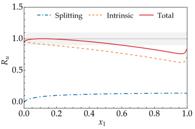
(a) $u$ momentum sum rule

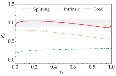
(b) $g$ momentum sum rule

Figure 1: Momentum sum rule ratios $R_{u}$ and $R_{g}$ for the initial model of section 3, evaluated at the scale $\mu_{\text{min}}=2.25\operatorname{GeV}$. Shown are the individual contributions from the intrinsic and splitting parts in (4), as well as the full result. The $\pm 10\%$ deviations from unity are indicated by a light grey band. Not shown is the separate contribution from the matching term $F_{\text{match}}$, which is negligible in this case. The remaining plots in this section will follow the same conventions unless explicitly stated otherwise.

Let us investigate at this point the phase space factor $\rho_{a_{1}a_{2}}$ in (9). In some of the earlier works on DPDs, a simple factor $(1-x_{1}-x_{2})$ has been suggested [85, 86, 87, 88], whilst the more recent study [89] argued that a factor $(1-x_{1}-x_{2})^{2}$ is more appropriate. Even higher powers $n$ would be obtained if one were to generalise the Brodsky-Farrar quark counting rules [90, 91] from PDFs to DPDs. Each of these variants leads to a very strong suppression of DPDs in the region where $x_{1}\approx 1$ and $x_{2}\approx 0$ (or vice versa), since in that region the suppression from the phase space factor comes on top of the suppression of the corresponding PDF. As discussed in section 3, it is more appropriate to divide $(1-x_{1}-x_{2})^{n}$ by $(1-x_{1})^{n}\,(1-x_{2})^{n}$ for a given $n$ in order to remove the phase space suppression in the regions $x_{1}\approx 0$ and $x_{2}\approx 0$. Including this division, we have investigated the momentum sum rules for different values of $n$ and find that best agreement is achieved for $n=2$, as is illustrated by the comparison of figure 2 with figure 1(b).

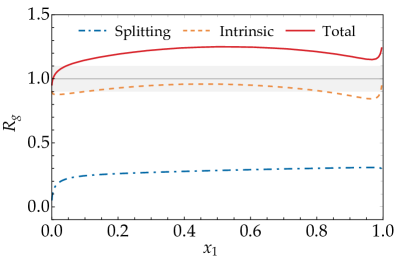
(a) $n=1$, $g$ momentum sum rule

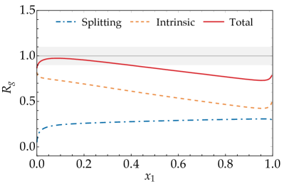
(b) $n=3$, $g$ momentum sum rule

Figure 2: The momentum sum rule ratio $R_{g}$ for different powers $n$ in the phase space factor $\rho_{a_{1}a_{2}}=(1-x_{1}-x_{2})^{n}\,(1-x_{1})^{-n}\,(1-x_{2})^{-n}$ of the intrinsic part (9). The case $n=2$ is shown in figure 1(b).

Turning to the number sum rules, we find that these are violated quite strongly in the initial model, as is illustrated in figure 3. The agreement does not improve with other choices of the power $n$ just discussed.

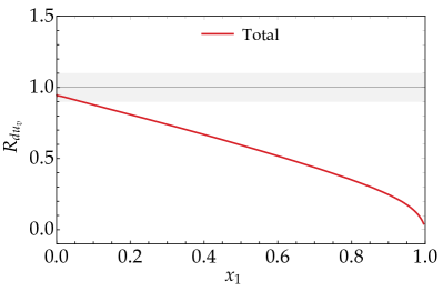
(a) $du_{v}$ number sum rule

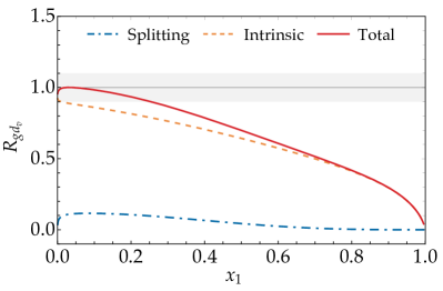
(b) $gd_{v}$ number sum rule

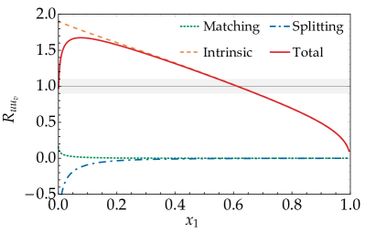
(c) $uu_{v}$ number sum rule

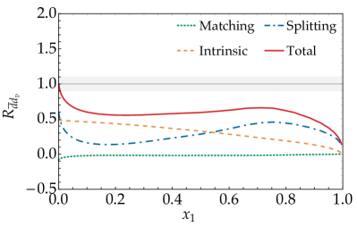
(d) $\bar{d}d_{v}$ number sum rule

Figure 3: Number sum rule ratios $R_{a_{1}q_{v}}$ for the initial model. The upper plots are for unequal flavors of the two partons, and the lower ones are for equal flavours. The ratio $R_{du_{v}}$ is completely dominated by the intrinsic part of the DPD.

The adjustments discussed in the following will improve the situation considerably. Let us at this point note that the number sum rules for equal quark flavours (such as those in the lower row of figure 3) can receive a substantial contribution from $g\to q\bar{q}$ splitting at the starting scale $\mu_{y}$ of $F_{\text{spl}}$. This contribution is negative for $a_{1}=q$ and positive for $a_{1}=\bar{q}$, given that $F_{a_{1}q_{v}}=F_{a_{1}q}-F_{a_{1}\bar{q}}$.

5.2 First iteration: number effects and modified phase space factor

In the first iteration of our model, we implement the same two adjustments that were already made in [77]. To describe these adjustments, it is convenient to specify the ansatz (9) for $F_{a_{1}a_{2},\mskip 1.5mu\text{int}}$ with $a_{1}$ and $a_{2}$ taking the values $q_{v},\bar{q},g$ instead of $q$, $\bar{q}$, $g$ (with $q_{v}$ denoting the linear combination $q-\bar{q}$). This switch from quarks and antiquarks to “valence” and “sea” quarks is familiar from the parametrisation of ordinary PDFs.

Following the argumentation in [77], it is natural to change the ansatz for distributions with two valence quark labels so as to take into account “number effects”, i.e. the fact that we have a finite number of valence quarks in the proton, two $u$ and one $d$. To do this, we set $F_{u_{v}u_{v},\text{int}}$ to half the value given by (9) and set $F_{d_{v}d_{v},\text{int}}$ to zero. The latter corresponds to the simple intuition that the probability to find two “valence $d$ quarks” in the proton is nil. The second adjustment argued for in [77] is to modify the phase space factor from the parton independent form in (10) to

$$\rho_{a_{1}a_{2}}(x_{1},x_{2})\, =(1-x_{1}-x_{2})^{2}\,(1-x_{1})^{-2-\alpha(a_{2})}\,(1-x_{2})^{-2-\alpha(a_{1})}\,,$$ (22)

with

$$\alpha(a)=\begin{cases}0.5&\text{for $a=q_{v}$}\\ 0&\text{for $a=\bar{q},g$}\end{cases}$$ (23)

Whilst the original form in (10) satisfies $0\leq\rho_{a_{1}a_{2}}\leq 1$, the phase space factor in (22) becomes greater than $1$ when the momentum fraction of a valence parton tends to $0$ and the momentum fraction of the other parton (valence or sea) tends to $1$. Due to the PDFs in the ansatz (9), the intrinsic part of the DPD still goes to zero in that limit.

With these modifications, we find that the momentum sum rules are further improved, such that for most of the $x_{1}$ range, relative deviations are less then $10\%$. This is illustrated in figure 4, which is to be compared with figure 1 for the initial model.

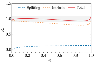
(a) $u$ momentum sum rule

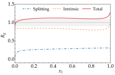
(b) $g$ momentum sum rule

Figure 4: Momentum sum rule ratios for the first iteration of our model, taking into account number effects (explained in the second paragraph of section 5.2) and the modified phase space factor given by (22) and (23). The corresponding plots for the original model are shown in figure 1.

A more significant improvement is obtained for the number sum rules, as can be seen from the comparison of figure 5 with figure 3. The modified phase space factor yields a weaker suppression for valence partons at large momentum fractions of the other parton. This largely mitigates the steep decrease of the sum rule ratios with $x_{1}$ in the initial model. Taking into account number effects strongly reduces the value of $R_{uu_{v}}$ at low $x_{1}$, which is much too high in figure 3(c).

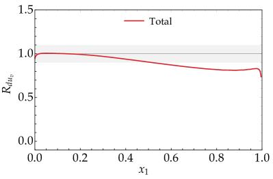
(a) $du_{v}$ number sum rule

(b) $gd_{v}$ number sum rule

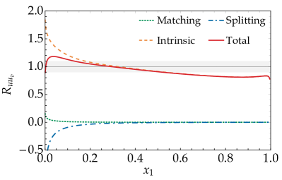
(c) $uu_{v}$ number sum rule

(d) $\bar{d}d_{v}$ number sum rule

Figure 5: The same number sum rule ratios as in figure 3, but for the first iteration of our model.

5.3 Second iteration: parameter scan for the phase space factor

Given that there is no strong motivation to take the particular value $0.5$ for $\alpha(u_{v})$ and $\alpha(d_{v})$ in (23), it is natural to explore whether tuning these parameters can improve the sum rule ratios further. We have therefore performed a parameter scan over these two powers. To quantify the degree to which the sum rules are fulfilled, we introduce

$$\delta =\int\limits_{x_{\text{min}}}^{0.8}\text{d}x_{1}\,\left|R(x_{1})-1\right|$$ (24)

as a quality measure for each sum rule ratio $R$, where $x_{\text{min}}=5\times 10^{-5}$. A global quality measure is then the sum $\delta_{\text{gl}}$ of these measures over all sum rules, excluding of course the cases for which $R_{a_{1}q_{v}}$ cannot be defined, as specified below (20).

Notice that in (24) we have taken an upper integration limit of $x_{1}=0.8$. This is because for very high $x_{1}$, we consider even large relative deviations from the DPD sum rules to be acceptable: DPDs in this region are expected to be very small and should hence not play any role in cross sections that are of measurable size.

The values of $\delta_{\text{gl}}$ obtained in our parameter scan over $\alpha(u_{v})$ and $\alpha(d_{v})$ are shown in figure 6. A minimum is reached at

$$\alpha(a)=\begin{cases}0.63&\text{for $a=u_{v}$}\\ 0.49&\text{for $a=d_{v}$}\\ 0&\text{for $a=\bar{q},g$}\\ \end{cases}$$ (25)

which we take as the second iteration of our model.

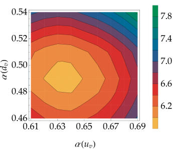
Figure 6: The quality measure $\delta_{\text{gl}}$ defined after (24), evaluated as a function of the powers $\alpha(u_{v})$ and $\alpha(d_{v})$ in the phase space factor. The right panel gives a zoom into the parameter space shown on the left.

As illustrated in figure 7(a), the momentum sum rules are not strongly affected by this change of parameters. The same holds for number sum rules that do not involve $u$ quarks, which is not surprising because $\alpha(u_{v})$ has significantly changed whereas $\alpha(d_{v})$ has not. Furthermore, we see in figure 7(b) that the change in $R_{ud_{v}}$ is very small. By contrast, all number sum rules for $u_{v}$ are significantly improved in the range $x_{1}\leq 0.8$, as illustrated in the lower plots of figure 7.

(a) $u$ momentum sum rule

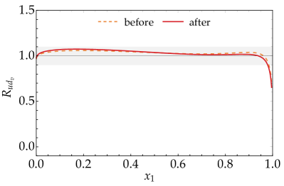
(b) $ud_{v}$ number sum rule

(c) $du_{v}$ number sum rule

(d) $uu_{v}$ number sum rule

Figure 7: Sum rule ratios in the first and second interactions of the model, which respectively correspond to the powers (23) and (25) in the phase space factor.

One may wonder whether tuning other parameters in our model can lead to further improvements. Candidates for such an endeavour are the parameter $y_{\text{max}}$ in the starting scale $\mu_{y}$ of $F_{\text{spl}}$, as well as the widths $h_{a_{1}a_{2}}$ of the Gaussian damping factor, which appears in both $F_{\text{int}}$ and $F_{\text{spl}}$. We find, however, that changing these parameters does not lead to a significant decrease of $\delta_{\text{gl}}$, and that the minimum of $\delta_{\text{gl}}$ is achieved for parameter values very close to those specified in section 3. We hence leave these parameters at their initial values.

Notice that the Gaussian factor in the intrinsic part (9) of the DPD is normalised such that its integral over all $\boldsymbol{y}$ gives unity. Restricting this integral to $y\geq b_{0}/\nu$ has little effect, which explains why a change of $h_{a_{1}a_{2}}$ has almost no impact on the contribution of $F_{\text{int}}$ to the sum rules.

5.4 Third iteration: modifying the splitting part at large distances

After several modifications to the intrinsic part $F_{\text{int}}$ of our DPD model, we now turn to the splitting part $F_{\text{spl}}$. While the latter can be computed for perturbatively small $y$, its form at large distance $y$ needs to be modelled. We now modify the initial ansatz (14) and multiply $F_{\text{spl,pt}}$ by the superposition of two Gaussians in $y$, with a relative weight depending on the momentum fractions:

$$\tilde{F}_{a_{1}a_{2},\text{spl}}(x_{1},x_{2},\boldsymbol{y};\mu_{y}) =F_{a_{1}a_{2},\text{spl,pt}}(x_{1},x_{2},\boldsymbol{y};\mu_{y})\exp\left[-\frac{y^{2}}{4h_{a_{1}a_{2}}}\right]$$

$$\quad\times\Biggl{\{}1+\left(\exp\left[\frac{y^{2}}{4h_{a_{1}a_{2}}^{*}}\right]-1\right)g_{a_{1}a_{2}}(x_{1}+x_{2})\Biggr{\}}\,.$$ (26)

The factor multiplying $F_{\text{spl,pt}}$ can be rewritten as the sum of two Gaussians, one multiplied with $1-g_{a_{1}a_{2}}(x_{1}+x_{2})$ and the other multiplied with $g_{a_{1}a_{2}}(x_{1}+x_{2})$. For the new width parameters $h_{a_{1}a_{2}}^{*}$ we make the same ansatz as we did for $h_{a_{1}a_{2}}^{\phantom{*}}$, i.e. we set $h_{a_{1}a_{2}}^{*}=h_{a_{1}}^{*}+h_{a_{2}}^{*}$. We take values

$$h_{g}^{*} =3.015\operatorname{GeV}^{-2}\,, h_{q}^{*}=h_{\bar{q}}^{*} =5.375\operatorname{GeV}^{-2}$$ (27)

such that the Gaussian factor $\exp\bigl{[}-y^{2}/(4h_{a_{1}a_{2}})+y^{2}/(4h_{a_{1}a_{2}}^{*})\bigr{]}$ multiplying $g_{a_{1}a_{2}}$ is approximately the same for all parton combinations. Admittedly, the form (5.4) is rather special among all possible functions that have the correct limit at small $y$. Clearly, the requirement of fulfilling the sum rules is not nearly enough to determine the functional form of DPDs at large $y$, so that a particular ansatz must be made. Our choice has the feature of introducing a nontrivial interplay between the dependence on $y$ and on the parton momentum fractions, controlled by a one-variable function $g_{a_{1}a_{2}}(x_{1}+x_{2})$ for each LO splitting process $a_{0}\to a_{1}a_{2}$. We will find that this is an adequate degree of complexity, in the sense that the sum rule constraints are sufficient to determine this function.

Whilst strict positivity of $\tilde{F}_{\text{spl}}$ requires $g_{a_{1}a_{2}}(x_{1}+x_{2})>0$, the procedure described below yields negative values of this function in some cases. We checked that the resulting full DPDs $F_{\text{int}}+\tilde{F}_{\text{spl}}$ are still positive in the range of $x_{1},x_{2}$ and $y$ covered by our DPD grids. This holds for all scales $\mu$ on our grid, from the starting scale $\mu_{\text{min}}=2.25\operatorname{GeV}$ up to the highest value $\mu=172\operatorname{GeV}$.

Let us first consider the splitting $g\to q\bar{q}$, where $q$ takes one of the values $u$, $d$, $s$. This splitting feeds into the number sum rules for equal quark flavours, which at this stage are least well satisfied. Judging the impact of the function $g_{a_{1}a_{2}}(x_{1}+x_{2})$ is complicated by the fact that the ansatz (5.4) for $\tilde{F}_{\text{spl}}$ is made at the $y$ dependent scale $\mu_{y}$ and needs to be evolved to the scale $\mu_{\min}$ where we evaluate the sum rules. For definiteness, we consider the sum rule

$$(N_{q_{v}}+1)\,f_{\bar{q}}(x_{1};\mu_{\text{min}}) =\int\limits_{0}^{1-x_{1}}\!\text{d}x_{2}\int\text{d}^{2}\boldsymbol{y}\;\Bigl{[}F_{\bar{q}q_{v},\text{int}}(x_{1},x_{2},\boldsymbol{y};\mu_{\text{min}})+\tilde{F}_{\bar{q}q_{v},\text{spl}}(x_{1},x_{2},\boldsymbol{y};\mu_{\text{min}})\Bigr{]}$$

$$\quad+\int\limits_{0}^{1-x_{1}}\!\text{d}x_{2}\;F_{\bar{q}q_{v},\text{match}}(x_{1},x_{2};\mu_{\text{min}})\,,$$ (28)

where here and in the following it is understood that the integrals over $\boldsymbol{y}$ are restricted to $y\geq b_{0}/\nu=b_{0}/\mu_{\text{min}}$. To simplify the determination of $g_{a_{1}a_{2}}(x_{1}+x_{2})$, we make two approximations. Firstly, we use that for small $y$ the initial and modified splitting model do not differ significantly, i.e.

$$\tilde{F}_{\bar{q}q_{v},\text{spl}}(x_{1},x_{2},\boldsymbol{y};\mu_{\text{min}})\approx F_{\bar{q}q_{v},\text{spl}}(x_{1},x_{2},\boldsymbol{y};\mu_{\text{min}})\,.$$ (29)

Secondly, we recall that for large $y$ the scale $\mu_{y}$ is close to $\mu_{\text{min}}$, so that we have

$$\tilde{F}_{\bar{q}q_{v},\text{spl}}(x_{1},x_{2},\boldsymbol{y};\mu_{\text{min}})\approx\tilde{F}_{\bar{q}q_{v},\text{spl}}(x_{1},x_{2},\boldsymbol{y};\mu_{y})\,.$$ (30)

Combining both approximations gives

$$\int\text{d}^{2}\boldsymbol{y}\,\tilde{F}_{\bar{q}q_{v},\text{spl}}(x_{1},x_{2},\boldsymbol{y};\mu_{\text{min}})\approx \int\text{d}^{2}\boldsymbol{y}\;\Theta(y_{\text{sep}}-y)\,F_{\bar{q}q_{v},\text{spl}}(x_{1},x_{2},\boldsymbol{y};\mu_{\text{min}})$$

$$+\int\text{d}^{2}\boldsymbol{y}\;\Theta(y-y_{\text{sep}})\,\tilde{F}_{\bar{q}q_{v},\text{spl}}(x_{1},x_{2},\boldsymbol{y};\mu_{y})\,,$$ (31)

where we use (29) below $y_{\text{sep}}$ and (30) above. Taking $y_{\text{sep}}=1\operatorname{GeV}^{-1}$ ensures that (30) is rather well fulfilled, as $\mu_{\text{min}}$ and $\mu_{y}$ differ by at most $12\%$. We will find that $|g_{q\bar{q}}|<12$, which corresponds to a relative discrepancy below $30\%$ between the l.h.s. and the r.h.s. of (29). While this may not seem to be very precise, it will turn out to be sufficient for improving the sum rules significantly.

Using (5.4) and (5.4), the sum rule (5.4) can be approximated as

$$k_{\bar{q}}(x_{1})\, \underset{\text{def}}{=}\,(N_{q_{v}}+1)\,f_{\bar{q}}(x_{1};\mu_{\text{min}})\;-\!\int\limits_{0}^{1-x_{1}}\!\text{d}x_{2}\;F_{\bar{q}q_{v}}(x_{1},x_{2};\mu_{\text{min}})$$

$$=\int\limits_{0}^{1-x_{1}}\!\text{d}x_{2}\int\text{d}^{2}\boldsymbol{y}\;\Theta(y-y_{\text{sep}})\,F_{q\bar{q},\text{spl}}(x_{1},x_{2},\boldsymbol{y};\mu_{y})\,h_{q\bar{q}}(y)\,g_{q\bar{q}}(x_{1}+x_{2})\,,$$ (32)

where $F_{\bar{q}q_{v}}(x_{1},x_{2};\mu)$ denotes the full DPD (4) in the second iteration of our model and we have abbreviated

$$h_{q\bar{q}}^{\phantom{*}}(y) =\exp\bigl{[}y^{2}/(4h_{q\bar{q}}^{*})\bigr{]}-1\,.$$ (33)

Here we used that at the scale $\mu_{y}$ one has ${F}_{\bar{q}q_{v},\text{spl}}={F}_{\bar{q}q,\text{spl}}={F}_{q\bar{q},\text{spl}}$ and a corresponding relation for $\tilde{F}_{a_{1}a_{2},\text{spl}}$. Shifting the integration variable on the r.h.s. of (5.4) from $x_{2}$ to $x=x_{1}+x_{2}$ gives

$$k_{\bar{q}}(x_{1}) =\int\limits_{1}^{x_{1}}\text{d}x\;K_{q\bar{q}}(x_{1},x)\,g_{q\bar{q}}(x)$$ (34)

with

$$K_{q\bar{q}}(x_{1},x) =-\int\text{d}^{2}\boldsymbol{y}\;\Theta(y-y_{\text{sep}})\,F_{q\bar{q},\text{spl}}(x_{1},x-x_{1},\boldsymbol{y};\mu_{y})\,h_{q\bar{q}}(y)\,.$$ (35)

We recognise in (34) a Volterra equation of the first kind [92]. We discretise this equation by taking both $x_{1}$ and $x$ on the grid for DPDs discussed in section 4. The integral over $x$ is turned into a sum using a simple trapezoidal rule in the variable $u=\log(x/(1-x))$. The result is a linear system of equations

$$(k_{\bar{q}})_{i}=\sum_{j}(K_{q\bar{q}})_{ij}\,(g_{q\bar{q}})_{j}$$ (36)

with an upper diagonal matrix $K_{ij}$, which is readily solved using Gauss-Jordan elimination.

In order to have an analytic formulation for our model, we fit the obtained discrete values of $g_{a_{1}a_{2}}(x)$ to the form

$$g(x) =A+Bx^{b}+C\mskip 1.5mux^{c_{1}}(1-x)^{c_{2}}\,,$$ (37)

for each of the splittings $g\to u\bar{u},g\to d\bar{d}$, and $g\to s\bar{s}$. This reproduces the general shape of the numerical results rather well, except for some deviations at very large $x$. The resulting functions are shown in figure 8(a) to 8(c), and the fitted parameters are given in table 1.

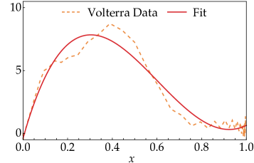
(a) $g_{u\bar{u}}$

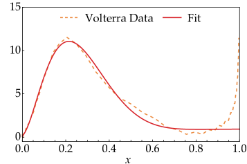
(b) $g_{d\bar{d}}$

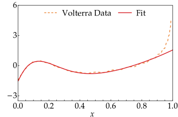
(c) $g_{s\bar{s}}$

(d) $g_{gg}$

Figure 8: Modification functions $g_{a_{1}a_{2}}(x)$ for the $g\to q\bar{q}$ and $g\to gg$ splittings. For each channel we display the fit to the form (37) and the direct solution of the discretised Volterra equation (36). The direct solution is shown as a dashed curve with linear interpolation between each data point.

$a_{0}\to a_{1}a_{2}$	$A$	$B$	$b$	$C$	$c_{1}$	$c_{2}$
$g\to u\bar{u}$	$-0.4193$	$1.0627$	$7.7448$	$60.8558$	$0.9881$	$2.2641$
$g\to d\bar{d}$	$-0.8020$	$1.7291$	$0.0988$	$932.0289$	$1.8515$	$6.8244$
$g\to s\bar{s}$	$-1.5409$	$3.0985$	$2.3609$	$49.8862$	$1.0964$	$7.2093$
$g\to gg$	$25.8143$	$-26.1923$	$0.0600$	$-5.3466$	$0.0764$	$2.6904$

Table 1: Parameters of the modification functions $g_{a_{1}a_{2}}$ defined by (5.4) and (37).

With these modified $g\to q\bar{q}$ splittings, the agreement of the model with the $\bar{q}q_{v}$ number sum rules improves significantly, as can be seen in figure 9(b) to 9(d). Remarkably, the modification of the $g\to u\bar{u}$ splitting improves not only the sum rule for $\bar{u}u_{v}$ but also one for $uu_{v}$, as seen in figure 9(a).

(a) $uu_{v}$ number sum rule

(b) $\bar{u}u_{v}$ number sum rule

(c) $\bar{d}d_{v}$ number sum rule

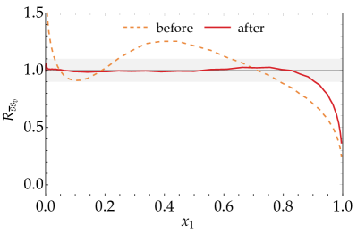
(d) $\bar{s}s_{v}$ number sum rule

Figure 9: Change of the number sum rules for equal flavours due to the modification of the $g\to q\bar{q}$ splittings at large $y$.

At this point, we recall that the ratio $R_{a_{1}q_{v}}$ is undefined for $F_{dd_{v}}$. In order to quantify how well the number sum rule for this distribution is satisfied, we introduce the modified ratio

$$\tilde{R}_{dd_{v}}(x_{1};\mu) =\frac{\int\mathrm{d}x_{2}\,F_{dd_{v}}(x_{1},x_{2};\mu)}{f_{d}(x_{1};\mu)}\,,$$ (38)

in which the zero prefactor in the denominator of (19) has been replaced with unity. The ratio $\tilde{R}_{dd_{v}}$ should be close to zero. We see in figure 10 that this is indeed the case: the modification of the $g\to d\bar{d}$ splitting improves not only the sum rule for $F_{\bar{d}d_{v}}$ but also the one for $F_{dd_{v}}$. Altogether, we have reached a satisfactory agreement of our model with all number sum rules.

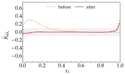
(a) $dd_{v}$ number sum rule

Figure 10: Change of the sum rule ratio (38) due to the modification of the $g\to d\bar{d}$ splitting at large $y$. The sum rule is exactly satisfied if $\tilde{R}_{dd_{v}}=0$.

The modification of the $g\to q\bar{q}$ splitting also affects the quark momentum sum rules, as illustrated in figure 11. In the cases shown in the figure, the agreement of the momentum sum rule becomes slightly worse, whereas the changes in the remaining cases are insignificant. One could improve $R_{\bar{u}}$ and $R_{\smash{\bar{d}}}$ by modifying the $g\to g\bar{u}$ and $g\to g\bar{d}$ splittings, but this would also affect the number sum rules ratios $R_{gu_{v}}$ and $R_{g\smash{d_{v}}}$. We refrain from such an exercise, considering that the agreement shown in figure 11 is still satisfactory.

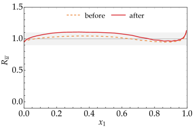
(a) $\bar{u}$ momentum sum rule

(b) $\bar{d}$ momentum sum rule

Figure 11: Change of momentum sum rules due to the modification of the $g\to q\bar{q}$ splittings at large $y$.

The sum rule ratio that is farthest away from $1$ after these improvements is the one for the gluon momentum sum rule. This can be adjusted by modifying the $g\to gg$ splitting at large $y$ in the same way as discussed for $g\to q\bar{q}$. The parameters of the modification function $g_{gg}(x)$ are given in table 1, and the function itself is shown in figure 8(d). The resulting improvement of the sum rule can be seen in figure 12, and we have checked that none of the other sum rule ratios is adversely affected by this final modification of our model.

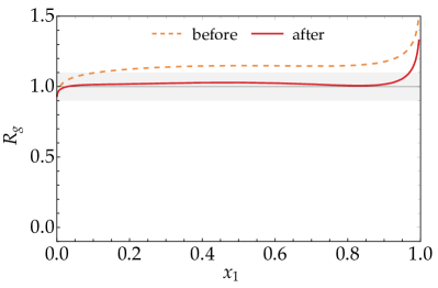
(a) $g$ momentum sum rule

Figure 12: Change of the gluon momentum sum rule due to the modification of the $g\to gg$ splitting at large $y$.

Let us finally take a look at the relative importance of intrinsic and splitting contributions to the sum rules in the final iteration of our model. In figures 13 and 14, we show the situation for the same sum rules that were shown in figures 1 and 3 for our initial model. We find that for $R_{u}$, $R_{du_{v}}$, and $R_{gd_{v}}$ the main change between the initial and final versions is due to the intrinsic part. By contrast, for $R_{g}$ and $R_{uu_{v}}$, and $R_{\smash{\bar{d}}d_{v}}$ there are important changes both in the intrinsic and in the splitting parts, where the latter are restricted to the small $x_{1}$ region in the case of $R_{uu_{v}}$. That these sum rules are strongly affected by the splitting modification at large $y$ was already seen in figures 12, 9(a), and 9(c).

In the final iteration of our model, the sum rules that receive positive or negative splitting contributions larger than $20\%$ in at least part of the $x_{1}$ range are the momentum sum rules for sea quarks ($\bar{u}$, $\bar{d}$, $\bar{s}$, and $s$) and the number sum rules for equal flavours ($qq_{v}$ and $\bar{q}q_{v}$). Compared with the initial model, the contribution of the $g\to gg$ splitting to $R_{g}$ has strongly decreased due to its modification at large $y$.

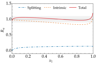
(a) $u$ momentum sum rule

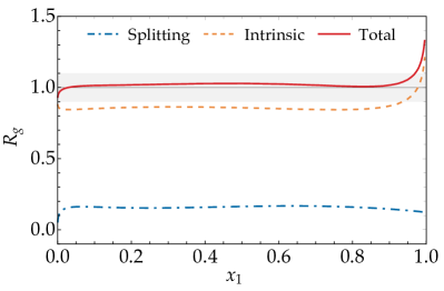
(b) $g$ momentum sum rule

Figure 13: Momentum sum rule ratios $R_{u}$ and $R_{g}$ for the final iteration of our model. The corresponding plots for the initial model are in figure 1 and those for the first iteration in figure 4. Not shown is the separate contribution from the matching term $F_{\text{match}}$, which is negligible in this case.

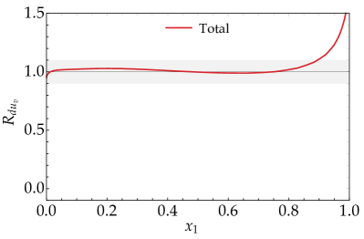
(a) $du_{v}$ number sum rule

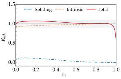
(b) $gd_{v}$ number sum rule

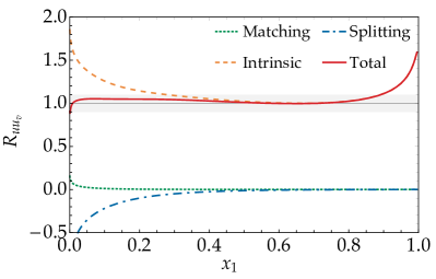
(c) $uu_{v}$ number sum rule

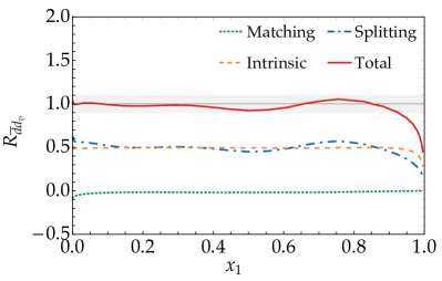
(d) $\bar{d}d_{v}$ number sum rule

Figure 14: Number sum rule ratios $R_{a_{1}q_{v}}$ for the final iteration of our model. The corresponding plots for the initial model are in figure 3 and those for the first iteration in figure 5.. The ratio $R_{du_{v}}$ is completely dominated by the intrinsic part of the DPD.

6 Scale dependence

So far, we have evaluated the sum rules for DPDs and PDFs at the scale $\mu=\mu_{\text{min}}=2.25\operatorname{GeV}$, and with the matching between position and momentum space DPDs computed for a cutoff scale $\nu=\mu$. In this section, we investigate how the sum rules change if these scales are chosen differently.

6.1 Renormalisation scale

As shown in [77], the DPD sum rules are preserved under LO evolution. If they are approximately valid at some scale, one may expect that they are still approximately valid when the DPDs and PDFs are evolved to a different scale. We verified that this is indeed the case for the DPD model developed in the previous section. This is illustrated in figure 15 for momentum sum rules and in figure 16 for number sum rules. We evolved the distributions from $\mu_{\text{min}}$ to $\mu=144.6\operatorname{GeV}$, which is a point on our $\mu$ grid. The DPD matching at the high scale is evaluated with $\nu=\mu$.

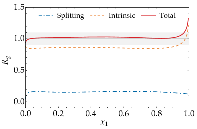
(a) $g$ momentum sum rule at $\mu=2.25\operatorname{GeV}$

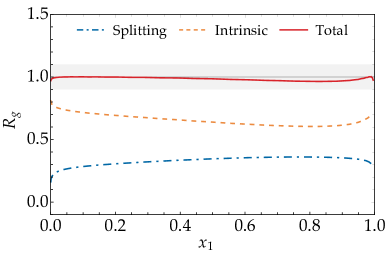
(b) $g$ momentum sum rule at $\mu=144.6\operatorname{GeV}$

Figure 15: Comparison of the gluon momentum sum rule ratio for the final iteration of our model at two different scales. The contribution of the matching term is small and not shown.

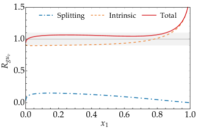
(a) $gu_{v}$ number sum rule at $\mu=2.25\operatorname{GeV}$

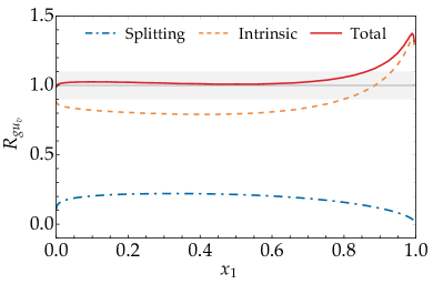
(b) $gu_{v}$ number sum rule at $\mu=144.6\operatorname{GeV}$

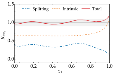
(c) $\bar{u}u_{v}$ number sum rule at $\mu=2.25\operatorname{GeV}$

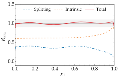
(d) $\bar{u}u_{v}$ number sum rule at $\mu=144.6\operatorname{GeV}$

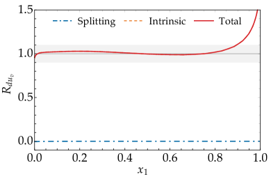
(e) $du_{v}$ number sum rule at $\mu=2.25\operatorname{GeV}$

(f) $du_{v}$ number sum rule at $\mu=144.6\operatorname{GeV}$

Figure 16: Comparison of number sum rule ratios for the final model at low and high scales. The contribution of the matching term is small and not shown.

In the case of the $g$ momentum and the $gu_{v}$ number sum rule, we notice that the individual contributions from $F_{\text{int}}$ and $F_{\text{spl}}$ to the sum rule ratios change considerably under evolution, while the sum of all contributions remains nearly the same. This highlights the relevance of the perturbative splitting mechanism for ensuring the scale independence of the DPD sum rules, which was pointed out in a number of different studies [70, 71, 78].

In the figures for the $\bar{u}u_{v}$ sum rule, we observe that the oscillatory behaviour of $R_{\bar{u}u_{v}}$, which is a consequence of the modified splitting term in our model, is less pronounced after evolution to $\mu=144.6\operatorname{GeV}$. This is a typical feature of scale evolution, which tends to “wash out” details of distributions when going from low to high scales.

6.2 Cutoff scale

The matching relation given in (2) is only accurate up to higher orders in $\alpha_{s}$ and up to power corrections in $\Lambda/\nu$. The higher order analysis in [82] reveals that the term of order $\alpha_{s}^{n}$ in the matching relation is accompanied by up to $n$ powers of $\log(\mu^{2}/\nu^{2})$. Varying $\nu$ around its “natural value” $\mu$ thus provides an estimate of higher order and power corrections in the matching relation. Following a widespread practice for scale variations, we vary $\nu$ between $\mu/2$ and $2\mu$, taking again $\mu=\mu_{\text{min}}$. The resulting variation of the sum rule ratios for our final DPD model is illustrated in figure 17.

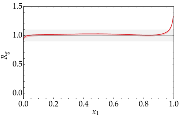
(a) $g$ momentum sum rule

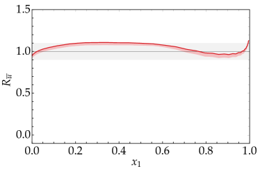
(b) $\bar{u}$ momentum sum rule

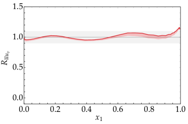
(c) $\bar{u}u_{v}$ number sum rule

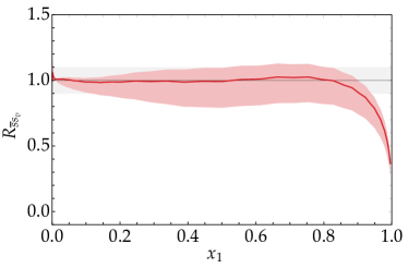
(d) $\bar{s}s_{v}$ number sum rule

Figure 17: Cutoff scale dependence of sum rule ratios, evaluated at $\mu=\mu_{\text{min}}$ for the final iteration of our model. The solid curve is for $\nu=\mu$, and the band corresponds to a variation of $\nu$ between $\mu/2$ and $2\mu$.

We find the $\nu$ dependence to be moderate, with changes of $10\%$ or less in the sum rule ratios in almost all cases. These variations are hence of the same order as the agreement of the sum rule ratios with $1$. The theoretical uncertainties reflected by the $\nu$ variation also suggest that it is of limited value to tune the sum rule ratios obtained for $\nu=\mu$ much further than we have done.

The only sum rule ratio with a larger $\nu$ dependence is $R_{\bar{s}s_{v}}$, shown in figure 17(d), which varies up to $20\%$. To understand this, we note that the $\nu$ dependence of the splitting and matching terms in (4) is stronger than the $\nu$ dependence of the intrinsic term. The latter gives an important contribution to all sum rule ratios, except for $R_{\bar{s}s_{v}}$, where within our model it is strictly zero.

One might wonder whether a change of the scale $\nu$ could systematically improve the agreement of our initial model with the sum rules. The examples in figure 18 show that this is not the case: the $\nu$ variation is not able to bring the ratios $R_{\bar{u}}$ or $R_{\bar{u}u_{v}}$ close to $1$ for all $x_{1}\leq 0.8$. We also note that the change of the sum rules with $\nu$ is roughly of the same size in our initial and final models. This justifies our choice of $\nu=\mu$ for the tuning of the model described in the previous section.

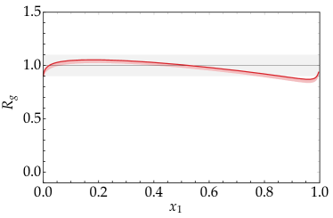
(a) $g$ momentum sum rule

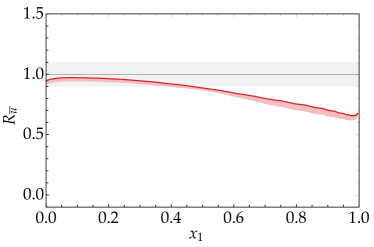
(b) $\bar{u}$ momentum sum rule

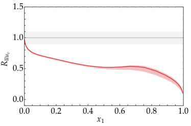
(c) $\bar{u}u_{v}$ number sum rule

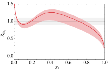
(d) $\bar{s}s_{v}$ number sum rule

Figure 18: As figure 17, but for the initial DPD model described in section 3.

7 Conclusions

The number and momentum sum rules for DPDs put important constraints on DPD parametrisations. We have shown that one can construct physically plausible models for DPDs in position space that approximately fulfil these constraints. Our starting point was the DPD ansatz used in [45], the construction of which ensures the correct small $y$ limit given by LO perturbation theory, but does not take into account DPD sum rule constraints at all. That ansatz was then sequentially modified: we started by adapting the modifications discussed in [77] to our case and furthermore tuned some model parameters, using parameter scans and a measure that quantifies how well the sum rules are globally satisfied. In the last step, we modified the form of the parton splitting term at large $y$, where perturbation theory is not applicable and this term has to be regarded as part of the non-perturbative model. Whilst the specific form of that modification was motivated more by practical considerations than by physical intuition, our exercise shows that one can adapt position space DPDs up to the point where all momentum and number sum rules are satisfied within about $10\%$ accuracy. An exception to this statement is the region of parton momentum fractions $x>0.8$, where even ordinary PDFs are poorly known and where double parton scattering processes will have tiny cross sections.

We verified that the approximate validity of the sum rules remains stable under evolution from low to high scales. Furthermore, we find that the sum rules are robust under variation of the cutoff scale $\nu$, which appears when converting DPDs from position to momentum space. The largest $\nu$ variation is observed for the number sum rule that involves only strange quarks, where we see effects of up to $20\%$. Since the $\nu$ variation reflects in particular the size of uncomputed higher orders in the parton splitting, and since we vary $\nu$ around a central value of $2.25\operatorname{GeV}$, we find a scale variation of this size not too surprising. One can expect that the inclusion of perturbative splitting terms at NLO, which have been computed in [82], will improve the situation.

For any given DPD model and PDF set, one can verify to which extent the sum rules are fulfilled. If they are violated significantly, one can unfortunately not fully deduce the region of variables $x_{1},x_{2},y$ in which the DPDs are unreliable, since the sum rules are integrated over one momentum fraction and over $y$. If, however, one has a given functional form of DPDs and needs to choose its parameters, the sum rules can be of more direct use. Whilst imposing that they be satisfied exactly will in general be a condition that cannot be fulfilled, the type of quality measure for the sum rules we introduced in section 5.3 provides a simple quantitative criterion for the theoretical consistency of the model. In a more sophisticated treatment, one should also take into account the uncertainties on the PDFs, which appear on the r.h.s. of the sum rules and typically are also an input to the DPD model.

Whilst perturbative calculations for double parton scattering have been pushed to higher orders in recent years, the construction of more reliable DPD models remains an outstanding task. The present work shows that two major theoretical constraints on DPDs, namely the small $y$ limit and the sum rules (where $y$ is integrated over) can be satisfied simultaneously at least in an approximate way. Of course, this theoretical input alone is not sufficient to pin down the DPDs, and ultimately, the predictions obtained with any DPD model should be compared with experiment. This will be a huge endeavour and must be left to future work.

References

- [1] A. Kulesza and W. J. Stirling, Like sign boson production at the LHC as a probe of double parton scattering, Phys. Lett. B475 (2000) 168 [hep-ph/9912232].
- [2] J. R. Gaunt, C.-H. Kom, A. Kulesza and W. J. Stirling, Same-sign W pair production as a probe of double parton scattering at the LHC, Eur. Phys. J. C69 (2010) 53 [1003.3953].
- [3] CMS collaboration, Double Parton Scattering cross section limit from same-sign bosons pair production in di-muon final state at LHC, CMS-PAS-FSQ-13-001 (2015).
- [4] F. A. Ceccopieri, M. Rinaldi and S. Scopetta, Parton correlations in same-sign pair production via double parton scattering at the LHC, Phys. Rev. D95 (2017) 114030 [1702.05363].
- [5] S. Cotogno, T. Kasemets and M. Myska, Spin on same-sign -boson pair production, Phys.Rev.D 100 (2019) 011503 [1809.09024].
- [6] CMS collaboration, A. M. Sirunyan et al., Evidence for WW production from double-parton interactions in proton–proton collisions at , Eur. Phys. J. C 80 (2020) 41 [1909.06265].
- [7] S. Cotogno, T. Kasemets and M. Myska, Confronting same-sign W-boson production with parton correlations, 2003.03347.
- [8] LHCb collaboration, R. Aaij et al., Measurement of the J/ pair production cross-section in pp collisions at TeV, JHEP 06 (2017) 047 [1612.07451].
- [9] CMS collaboration, V. Khachatryan et al., Search for new physics in same-sign dilepton events in proton-proton collisions at , Eur. Phys. J. C76 (2016) 439 [1605.03171].
- [10] CMS collaboration, A. M. Sirunyan et al., Search for top quark partners with charge 5/3 in the same-sign dilepton and single-lepton final states in proton-proton collisions at TeV, JHEP 03 (2019) 082 [1810.03188].
- [11] LHCb collaboration, R. Aaij et al., Observation of -pair production in collisions at = 7 TeV, Phys. Lett. B 707 (2012) 52 [1109.0963].
- [12] LHCb collaboration, R. Aaij et al., Observation of double charm production involving open charm in pp collisions at = 7 TeV, JHEP 06 (2012) 141 [1205.0975].
- [13] LHCb collaboration, R. Aaij et al., Production of associated and open charm hadrons in pp collisions at and 8 TeV via double parton scattering, JHEP 07 (2016) 052 [1510.05949].
- [14] ATLAS collaboration, G. Aad et al., Measurement of hard double-parton interactions in + 2-jet events at =7 TeV with the ATLAS detector, New J. Phys. 15 (2013) 033038 [1301.6872].
- [15] ATLAS collaboration, G. Aad et al., Measurement of the production cross section of prompt mesons in association with a boson in collisions at 7 TeV with the ATLAS detector, JHEP 04 (2014) 172 [1401.2831].
- [16] ATLAS collaboration, G. Aad et al., Observation and measurements of the production of prompt and non-prompt mesons in association with a boson in collisions at = 8 TeV with the ATLAS detector, Eur. Phys. J. C 75 (2015) 229 [1412.6428].
- [17] ATLAS collaboration, M. Aaboud et al., Study of hard double-parton scattering in four-jet events in collisions at TeV with the ATLAS experiment, JHEP 11 (2016) 110 [1608.01857].
- [18] ATLAS collaboration, M. Aaboud et al., Measurement of the prompt pair production cross-section in collisions at TeV with the ATLAS detector, Eur. Phys. J. C 77 (2017) 76 [1612.02950].
- [19] ATLAS collaboration, M. Aaboud et al., Study of the hard double-parton scattering contribution to inclusive four-lepton production in collisions at 8 TeV with the ATLAS detector, Phys. Lett. B790 (2019) 595 [1811.11094].
- [20] CMS collaboration, S. Chatrchyan et al., Study of double parton scattering using W + 2-jet events in proton-proton collisions at = 7 TeV, JHEP 03 (2014) 032 [1312.5729].
- [21] CMS collaboration, V. Khachatryan et al., Observation of (1S) pair production in proton-proton collisions at TeV, JHEP 05 (2017) 013 [1610.07095].
- [22] Axial Field Spectrometer collaboration, T. Akesson et al., Double Parton Scattering in Collisions at GeV, Z. Phys. C 34 (1987) 163.
- [23] UA2 collaboration, J. Alitti et al., A study of multi-jet events at the CERN p collider and a search for double parton scattering, Phys. Lett. B 268 (1991) 145.
- [24] CDF collaboration, F. Abe et al., Study of four-jet events and evidence for double parton interactions in collisions at TeV, Phys. Rev. D 47 (1993) 4857.
- [25] CDF collaboration, F. Abe et al., Measurement of Double Parton Scattering in Collisions at TeV, Phys. Rev. Lett. 79 (1997) 584.
- [26] CDF collaboration, F. Abe et al., Double parton scattering in collisions at TeV, Phys. Rev. D 56 (1997) 3811.
- [27] D0 collaboration, V. M. Abazov et al., Double parton interactions in +3 jet events in collisions at TeV, Phys. Rev. D 81 (2010) 052012 [0912.5104].
- [28] D0 collaboration, V. M. Abazov et al., Azimuthal decorrelations and multiple parton interactions in +2 jet and +3 jet events in collisions at TeV, Phys. Rev. D 83 (2011) 052008 [1101.1509].
- [29] D0 collaboration, V. M. Abazov et al., Double parton interactions in jet and jet jet events in collisions at TeV, Phys. Rev. D 89 (2014) 072006 [1402.1550].
- [30] D0 collaboration, V. M. Abazov et al., Observation and studies of double production at the Tevatron, Phys. Rev. D 90 (2014) 111101 [1406.2380].
- [31] D0 collaboration, V. M. Abazov et al., Evidence for Simultaneous Production of and Mesons, Phys. Rev. Lett. 116 (2016) 082002 [1511.02428].
- [32] D0 collaboration, V. M. Abazov et al., Study of double parton interactions in diphoton + dijet events in collisions at TeV, Phys. Rev. D 93 (2016) 052008 [1512.05291].
- [33] I. Belyaev and D. Savrina, Study of double parton scattering processes with heavy quarks, Adv. Ser. Direct. High Energy Phys. 29 (2018) 141 [1711.10877].
- [34] B. Blok, Yu. Dokshitzer, L. Frankfurt and M. Strikman, The Four jet production at LHC and Tevatron in QCD, Phys. Rev. D83 (2011) 071501 [1009.2714].
- [35] M. Diehl and A. Schäfer, Theoretical considerations on multiparton interactions in QCD, Phys. Lett. B698 (2011) 389 [1102.3081].
- [36] J. R. Gaunt and W. J. Stirling, Double Parton Scattering Singularity in One-Loop Integrals, JHEP 06 (2011) 048 [1103.1888].
- [37] M. G. Ryskin and A. M. Snigirev, A Fresh look at double parton scattering, Phys. Rev. D83 (2011) 114047 [1103.3495].
- [38] B. Blok, Yu. Dokshitser, L. Frankfurt and M. Strikman, pQCD physics of multiparton interactions, Eur. Phys. J. C72 (2012) 1963 [1106.5533].
- [39] M. Diehl, D. Ostermeier and A. Schäfer, Elements of a theory for multiparton interactions in QCD, JHEP 03 (2012) 089 [1111.0910].
- [40] A. V. Manohar and W. J. Waalewijn, A QCD Analysis of Double Parton Scattering: Color Correlations, Interference Effects and Evolution, Phys. Rev. D85 (2012) 114009 [1202.3794].
- [41] A. V. Manohar and W. J. Waalewijn, What is Double Parton Scattering?, Phys. Lett. B713 (2012) 196 [1202.5034].
- [42] M. G. Ryskin and A. M. Snigirev, Double parton scattering in double logarithm approximation of perturbative QCD, Phys. Rev. D86 (2012) 014018 [1203.2330].
- [43] M. Diehl and J. R. Gaunt, Double parton scattering theory overview, Adv. Ser. Direct. High Energy Phys. 29 (2018) 7 [1710.04408].
- [44] M. Diehl, J. R. Gaunt, D. Ostermeier, P. Plößl and A. Schäfer, Cancellation of Glauber gluon exchange in the double Drell-Yan process, JHEP 01 (2016) 076 [1510.08696].
- [45] M. Diehl, J. R. Gaunt and K. Schönwald, Double hard scattering without double counting, JHEP 06 (2017) 083 [1702.06486].
- [46] M. G. A. Buffing, M. Diehl and T. Kasemets, Transverse momentum in double parton scattering: factorisation, evolution and matching, JHEP 01 (2018) 044 [1708.03528].
- [47] M. Diehl and R. Nagar, Factorisation of soft gluons in multiparton scattering, JHEP 04 (2019) 124 [1812.09509].
- [48] G. T. Bodwin, Factorization of the Drell-Yan Cross-Section in Perturbation Theory, Phys. Rev. D31 (1985) 2616.
- [49] J. C. Collins, D. E. Soper and G. F. Sterman, Factorization for Short Distance Hadron-Hadron Scattering, Nucl. Phys. B261 (1985) 104.
- [50] J. C. Collins, D. E. Soper and G. F. Sterman, Soft Gluons and Factorization, Nucl. Phys. B308 (1988) 833.
- [51] H.-M. Chang, A. V. Manohar and W. J. Waalewijn, Double Parton Correlations in the Bag Model, Phys. Rev. D87 (2013) 034009 [1211.3132].
- [52] M. Rinaldi, S. Scopetta and V. Vento, Double parton correlations in constituent quark models, Phys. Rev. D87 (2013) 114021 [1302.6462].
- [53] W. Broniowski and E. Ruiz Arriola, Valence double parton distributions of the nucleon in a simple model, Few Body Syst. 55 (2014) 381 [1310.8419].
- [54] M. Rinaldi, S. Scopetta, M. Traini and V. Vento, Double parton correlations and constituent quark models: a Light Front approach to the valence sector, JHEP 12 (2014) 028 [1409.1500].
- [55] W. Broniowski, E. Ruiz Arriola and K. Golec-Biernat, Generalized Valon Model for Double Parton Distributions, Few Body Syst. 57 (2016) 405 [1602.00254].
- [56] T. Kasemets and A. Mukherjee, Quark-gluon double parton distributions in the light-front dressed quark model, Phys. Rev. D94 (2016) 074029 [1606.05686].
- [57] M. Rinaldi, S. Scopetta, M. C. Traini and V. Vento, Correlations in Double Parton Distributions: Perturbative and Non-Perturbative effects, JHEP 10 (2016) 063 [1608.02521].
- [58] M. Rinaldi and F. A. Ceccopieri, Relativistic effects in model calculations of double parton distribution function, Phys. Rev. D95 (2017) 034040 [1611.04793].
- [59] M. Rinaldi, S. Scopetta, M. Traini and V. Vento, A model calculation of double parton distribution functions of the pion, Eur. Phys. J. C78 (2018) 781 [1806.10112].
- [60] A. Courtoy, S. Noguera and S. Scopetta, Double parton distributions in the pion in the Nambu-Jona-Lasinio model, JHEP 12 (2019) 045 [1909.09530].
- [61] W. Broniowski and E. Ruiz Arriola, Double parton distribution of valence quarks in the pion in chiral quark models, Phys. Rev. D 101 (2020) 014019 [1910.03707].
- [62] W. Broniowski and E. Ruiz Arriola, Double parton distributions of the pion in the NJL model, in Light Cone 2019 (LC2019) Palaiseau, France, September 16-20, 2019, 2020, 2001.00883.
- [63] G. S. Bali, P. C. Bruns, L. Castagnini, M. Diehl, J. R. Gaunt, B. Gläßle et al., Two-current correlations in the pion on the lattice, JHEP 12 (2018) 061 [1807.03073].
- [64] C. Zimmermann, Two-current correlations and DPDs for the nucleon on the lattice, 1911.05051.
- [65] R. Kirschner, Generalized Lipatov-Altarelli-Parisi Equations and Jet Calculus Rules, Phys. Lett. B84 (1979) 266.
- [66] V. P. Shelest, A. M. Snigirev and G. M. Zinovev, The Multiparton Distribution Equations in QCD, Phys. Lett. B113 (1982) 325.
- [67] A. M. Snigirev, Double parton distributions in the leading logarithm approximation of perturbative QCD, Phys. Rev. D68 (2003) 114012 [hep-ph/0304172].
- [68] F. A. Ceccopieri, An update on the evolution of double parton distributions, Phys. Lett. B697 (2011) 482 [1011.6586].
- [69] J. R. Gaunt, Single Perturbative Splitting Diagrams in Double Parton Scattering, JHEP 01 (2013) 042 [1207.0480].
- [70] B. Blok, Yu. Dokshitzer, L. Frankfurt and M. Strikman, Perturbative QCD correlations in multi-parton collisions, Eur. Phys. J. C74 (2014) 2926 [1306.3763].
- [71] F. A. Ceccopieri, A second update on double parton distributions, Phys. Lett. B734 (2014) 79 [1403.2167].
- [72] A. M. Snigirev, N. A. Snigireva and G. M. Zinovjev, Perturbative and nonperturbative correlations in double parton distributions, Phys. Rev. D90 (2014) 014015 [1403.6947].
- [73] K. Golec-Biernat and E. Lewandowska, Electroweak boson production in double parton scattering, Phys. Rev. D90 (2014) 094032 [1407.4038].
- [74] J. R. Gaunt, R. Maciula and A. Szczurek, Conventional versus single-ladder-splitting contributions to double parton scattering production of two quarkonia, two Higgs bosons and , Phys. Rev. D90 (2014) 054017 [1407.5821].
- [75] K. Golec-Biernat and A. M. Stasto, Unintegrated double parton distributions, Phys. Rev. D95 (2017) 034033 [1611.02033].
- [76] E. Elias, K. Golec-Biernat and A. M. Staśto, Numerical analysis of the unintegrated double gluon distribution, JHEP 01 (2018) 141 [1801.00018].
- [77] J. R. Gaunt and W. J. Stirling, Double Parton Distributions Incorporating Perturbative QCD Evolution and Momentum and Quark Number Sum Rules, JHEP 03 (2010) 005 [0910.4347].
- [78] M. Diehl, P. Plößl and A. Schäfer, Proof of sum rules for double parton distributions in QCD, Eur. Phys. J. C79 (2019) 253 [1811.00289].
- [79] K. Golec-Biernat and E. Lewandowska, How to impose initial conditions for QCD evolution of double parton distributions?, Phys. Rev. D90 (2014) 014032 [1402.4079].
- [80] K. Golec-Biernat, E. Lewandowska, M. Serino, Z. Snyder and A. M. Stasto, Constraining the double gluon distribution by the single gluon distribution, Phys. Lett. B750 (2015) 559 [1507.08583].
- [81] B. Cabouat, J. R. Gaunt and K. Ostrolenk, A Monte-Carlo Simulation of Double Parton Scattering, JHEP 11 (2019) 061 [1906.04669].
- [82] M. Diehl, J. R. Gaunt, P. Plößl and A. Schäfer, Two-loop splitting in double parton distributions, SciPost Phys. 7 (2019) 017 [1902.08019].
- [83] L. Frankfurt, M. Strikman and C. Weiss, Dijet production as a centrality trigger for collisions at CERN LHC, Phys. Rev. D69 (2004) 114010 [hep-ph/0311231].
- [84] A. D. Martin, W. J. Stirling, R. S. Thorne and G. Watt, Parton distributions for the LHC, Eur. Phys. J. C63 (2009) 189 [0901.0002].
- [85] C. Goebel, F. Halzen and D. M. Scott, Double Drell-Yan Annihilations in Hadron Collisions: Novel Tests of the Constituent Picture, Phys. Rev. D22 (1980) 2789.
- [86] B. Humpert, Are there multi-quark interactions?, Phys. Lett. 131B (1983) 461.
- [87] B. Humpert and R. Odorico, Multiparton Scattering and QCD Radiation as Sources of Four Jet Events, Phys. Lett. 154B (1985) 211.
- [88] F. Halzen, P. Hoyer and W. J. Stirling, Evidence for Multiple Parton Interactions From the Observation of Multi-Muon Events in Drell-Yan Experiments, Phys. Lett. B188 (1987) 375.
- [89] V. L. Korotkikh and A. M. Snigirev, Double parton correlations versus factorized distributions, Phys. Lett. B594 (2004) 171 [hep-ph/0404155].
- [90] S. J. Brodsky and G. R. Farrar, Scaling Laws at Large Transverse Momentum, Phys. Rev. Lett. 31 (1973) 1153.
- [91] S. J. Brodsky and G. R. Farrar, Scaling Laws for Large Momentum Transfer Processes, Phys. Rev. D11 (1975) 1309.
- [92] T. Lalescu, Introduction à la théorie des équations intégrales. Librairie Scientifique A. Hermann, 1912.