Rate of estimation for the stationary distribution of stochastic damping Hamiltonian systems with continuous observations

Abstract.

We study the problem of the non-parametric estimation for the density $\pi$ of the stationary distribution of a stochastic two-dimensional damping Hamiltonian system $(Z_{t})_{t\in[0,T]}=(X_{t},Y_{t})_{t\in[0,T]}$. From the continuous observation of the sampling path on $[0,T]$, we study the rate of estimation for $\pi(x_{0},y_{0})$ as $T\to\infty$. We show that kernel based estimators can achieve the rate $T^{-v}$ for some explicit exponent $v\in(0,1/2)$. One finding is that the rate of estimation depends on the smoothness of $\pi$ and is completely different with the rate appearing in the standard i.i.d. setting or in the case of two-dimensional non degenerate diffusion processes. Especially, this rate depends also on $y_{0}$. Moreover, we obtain a minimax lower bound on the $L^{2}$-risk for pointwise estimation, with the same rate $T^{-v}$, up to $\log(T)$ terms.

1. Introduction

The class of hypo-elliptic diffusion processes, for which the diffusion coefficient is degenerate, has been the subject of many recent works and is used for modeling in many fields, such as mathematical finance, biology, neuro-science, mechanics, ecology,… (see e.g. [8], [11], [7] and references therein). In this paper, we focus on the situation of a bi-dimensional hypo-elliptic process, describing the evolution in time of the couple position/velocity of some quantity. The velocity $Y$ is modeled by a non degenerate one-dimensional diffusion process, while the position $X$ is its integral, and the resulting bi-dimensional process $Z=(X,Y)$ is hypo-elliptic. Our aim is to estimate the density $\pi$ of the stationary measure of this diffusion process, under the assumption of an ergodic setting.

The problem of non-parametric estimation of the stationary measure of a continuous mixing process is a long-standing problem (see for instance N’Guyen [13], or Comte and Merlevede [3] and references therein). Based on sample of length $T$ of the data Comte and Merlevede [3] find estimators of the stationary measure, converging at rate depending on the smoothness of the stationary measure and slower than $\sqrt{T}$, as it is usual in non-parametric problems.

In the specific context where the continuous time process is a one-dimensional diffusion process, observed continuously on some interval $[0,T]$, the finding is different. It is shown that the rate of estimation of the stationary measure is $\sqrt{T}$ (see Kutoyants [10]). The rate of estimation is thus independent of the smoothness of the object that one estimates, in contrast to the typical non-parametric situation. The optimal estimator is very specific to the diffusive nature of the process as it relies on the local time of the process. Remark that if the process is a diffusion observed discretely on $[0,T]$ with a sufficiently high frequency it is possible to estimate with rate $\sqrt{T}$ also (see [12], [4]).

The case of multi-dimensional non-degenerate diffusions is treated in Dalalyan and Reiß [6] and Srauss [14]. In that case, the local time process is not available, but it is shown that for non degenerate diffusion process of dimension $d=2$, there exists an estimator of the pointwise values of the stationary measure with rate $\sqrt{T}/\log(T)^{2}$. This rate of estimation does not depend on the smoothness of the stationary measure for $d=2$. In the situation of a non degenerate diffusion with dimension $d\geq 3$, they find estimators whose rate is polynomial in $T$, depends on both the smoothness of the stationary measure and the dimension $d\geq 3$. For $d\geq 3$, the rate is strictly slower than $\sqrt{T}$, but faster than the rate appearing in standard multivariate density estimation from $T$ i.i.d. observations. Hence, for $d\geq 3$, the diffusive structure of the process, enables to get a faster estimation rate than for the i.i.d. case, as well.

In the case of hypo-elliptic processes, fewer results exist for the estimation of the stationary distribution. In [5], the authors consider the case of two-dimensional process $Z=(X,Y)$, where $Y$ is a velocity and $X$ a position. Based on a discrete sampling of the path of size $n$, they propose an estimator of the stationary measure which converges at a non parametric rate depending on the smoothness of the stationary measure. Assuming that the stationary measure has anisotropic regularity $(k_{1},k_{2})$, the proposed estimator has a rate depending on the harmonic mean $2/(1/k_{1}+1/k_{2})$ as it is for the optimal rate of estimation of distribution on in the case of i.i.d. sequence.

In this paper, we focus on the situation where the process is observed continuously on $[0,T]$ and our goal is to determine what is the optimal rate of estimation of $\pi$ in this context. Assuming that the stationary density $(x,y)\mapsto\pi(x,y)$ has an anisotropic Hölder regularity with index $k_{1}$ with respect to the variable $x$, and $k_{2}$ with respect to $y$, we construct an estimator of $\pi(x_{0},y_{0})$ based on $(X_{t},Y_{t})_{t\in[0,T]}$. This estimator achieves some rate $T^{-v(k_{1},k_{2})}$ and this rate of convergence depends on the smoothness of $\pi$ in a very specific way. Indeed, the expression of the rate of estimation involves only $k_{1}$ or $k_{2}$, depending on the relative positions of these two smoothness indexes. This shows the specificity of the estimation problem for continuous observation of process $Z=(X,Y)$ with a non degenerate diffusive velocity $Y$, and a degenerate component $X$. It is noteworthy that we find a rate of estimation slower than in the case of continuous observation of a non-degenerate diffusion in dimension $2$. Another interesting finding is that the rate of estimation of $\pi(x_{0},y_{0})$ depends on the point where one estimates the stationary measure, and is slower for points corresponding to null velocity $y_{0}=0$. A crucial ingredient in the study of the rate of estimation is to derive the variance of a kernel estimator with a choice of bandwidth $(h_{1},h_{2})$. We show that the variance of the kernel estimator depends in a completely unsymmetrical way on $h_{1}$ and $h_{2}$. As a consequence, we get that the optimal bandwidth choice for the estimator is such that one of the two bandwidth can go almost arbitrarily fast to $0$, while the optimal choice for the other bandwidth depends sharply on the smoothness of the stationary measure.

Also, we show a lower bound for the minimax risk of estimation of $\pi(x_{0},y_{0})$ on a class of hypo-elliptic diffusion models with stationary measure of Hölder regularity $(k_{1},k_{2})$. This proves that it is impossible to estimate uniformly on this class with a rate faster than $T^{-v(k_{1},k_{2})}$ (up to $\log(T)$ term).

The outline of the paper is the following. In Section 2, we present the model and give assumptions that are sufficient to get an ergodic system with stationary measure admitting a density $\pi$. In Section 3, we present the construction of the estimator and states the results on their rate of convergence (in Theorem 1 for $y_{0}\neq 0$, and Theorem 2 for $y_{0}=0$). In Section 4, we prove the upper bound on the variance of the kernel estimator. We also illustrate the very specific behaviour of the variance of the kernel estimator for hypo-elliptic diffusion by numerical simulations. In Section 5, we state and prove minimax lower bounds for the risk of estimation. In the Appendix, we prove some technical results used in the proofs of Section 4.

2. Hamiltonian system and mixing property

Let us consider $(\Omega,\mathcal{A},\mathbb{P})$, some probability space on which a standard one dimensional Brownian motion $(B_{t})_{t\geq 0}$ is defined. We assume that the process $(Z_{t})_{t\geq 0}=(X_{t},Y_{t})_{t\geq 0}$ is solution of the stochastic differential equation

(2.1) $$\text{d}X_{t}=Y_{t}\text{d}t$$

(2.2) $$\text{d}Y_{t}=a(X_{t},Y_{t})\text{d}B_{t}-[\beta(X_{t},Y_{t})Y_{t}+V^{\prime}(X_{t})]\text{d}t,$$

where $(X_{0},Y_{0})$ is a random variable independent of $(B_{t})_{t}$.

We introduce the following regularity assumption on the coefficients.

Assumption HReg:

• The functions $a:\mathbb{R}^{2}\to\mathbb{R}$ is a $\mathcal{C}^{\infty}$ function and $\overline{a}>a(x,y)\geq\underline{a}>0$, and for some constants $\overline{a}>\underline{a}>0$.

• The function $\beta:\mathbb{R}^{2}\to\mathbb{R}$ is continuously differentiable, and such that ${\left|\beta(x,y)\right|}\leq\overline{\beta}$ for all $(x,y)\in\mathbb{R}^{2}$, and for some constant $\overline{\beta}>0$. Moreover, we have $\beta(x,y)>\underline{\beta}$, $\forall x\in[l,\infty),y\in\mathbb{R}$, where $l\geq 0$, $\underline{\beta}>0$ are two constants.

• The function $V:\mathbb{R}\to\mathbb{R}$ is lower bounded, and with $\mathcal{C}^{2}$ regularity.

It is shown in [17], that under the assumptions HReg the S.D.E. (2.1)–(2.2) admits a weak solution, which satisfies the Markov property, and the associated semi group $(P_{t})_{t\geq 0}$ is strongly Feller [17], which in turn implies that the process is strongly Markovian. Let us stress that the sign condition on $\beta$ for large $x$ together with the existence of lower bound on $V$ are crucial to insure that the solution of (2.1)–(2.2) does not explode in finite time. Of course, if we know that $(x,y)\mapsto a(x,y)$, $(x,y)\mapsto y\beta(x,y)$ and $x\mapsto V^{\prime}(x)$ are globally Lipschitz, the solutions of the S.D.E. exists in the strong sense.

We now introduce an assumption on the potential $V$ of the system that ensure that the process tends to some equilibrium.

Assumption HErg: one has $\displaystyle\lim_{{\left|x\right|}\to\infty}V^{\prime}(x)\text{sign}(x)=+\infty$.

Is is shown in [17] that under HReg and HErg, one can construct a Lyapounov function $\Psi\geq 1$, and that a stationary probability $\pi$ exists and is unique for the process $Z=(X,Y)$, and satisfies $\pi(\Psi)<\infty$. It is shown in [17] (see Theorem 2.4) that for some $D>0$ and $\rho>0$,

(2.3) $$\forall t\geq 0,\quad\forall z\in\mathbb{R}^{2},\quad\sup_{{\left|f\right|}\leq\Psi}{\left|P_{t}(f)(z)-\int_{\mathbb{R}^{2}}f(z^{\prime})\pi(\text{d}z^{\prime})\right|}\leq D\Psi(z)e^{-\rho t}$$

for any function measurable function $f$ such as $f/\Psi$ is bounded on $\mathbb{R}$ and where $(P_{t})_{t\geq 0}$ is the semi group of $Z$,

$$P_{t}(f)(z)=E[f(X_{t},Y_{t})\mid(X_{0},Y_{0})=z].$$

Remark that under HReg and HErg, it is possible to construct a Lyapounov function such that $\Psi(x,y)\geq\frac{1}{C}\exp\left(\frac{1}{C}[{\left|y\right|}^{2}+V(x)]\right)$, for some constant $C>0$ (see (3.10) in [17]). As a consequence, (2.3) applies to functions $f$ with exponential growth, and the invariant distribution admits finite exponential moments.

Hence, we can state the following proposition

Proposition 1.

Assume that the coefficients of the equation (2.2) satisfy HReg and HErg, then there exists a stationary solution $Z=(X,Y)$ to the S.D.E. (2.1)–(2.2), and the stationary distribution is unique and admits some density $\pi$. Moreover, there exist constants $D_{\text{erg}}>0$ and $\rho>0$ such that for any bounded measurable functions $f$, $g$, we have

(2.4) $$\forall t\geq 0,\quad{\left|\text{cov}(f(Z_{0}),g(Z_{t}))\right|}\leq{D_{\text{erg}}}{\left\lVert f\right\rVert}_{\infty}{\left\lVert g\right\rVert}_{\infty}e^{-\rho t}.$$

The Proposition (1) is a consequence of the results shown in [17]. Indeed, from the fact that the Lyapounov function $\Psi$ is greater than $1$ and integrable with respect to the stationary measure, one can check that (2.4) is a consequence of (2.3).

3. Estimator and upper bounds

In this section we introduce the expression for our estimator of the stationary measure $\pi$ of the S.D.E. (2.1)–(2.2) and prove that the estimator achieves some rate of convergence, depending on the smoothness of $\pi$.

Let $\varphi:\mathbb{R}\to\mathbb{R}$ a bounded, compactly supported function. For convenience, we suppose that the support of $\varphi$ is $[-1,1]$. We assume that

(3.1) $$\int_{\mathbb{R}}\varphi(u)\text{d}u=1,\quad\int_{\mathbb{R}}\varphi(u)u^{l}\text{d}u=0,\text{ for $l\in\{1,\dots,L\}$ where $L\geq 1$.}$$

We let $h_{1}(T)>0$, $h_{2}(T)>0$ be two bandwidths which converge to zero as $T\to\infty$, and we consider a kernel estimator of $\pi$ at the point $(x_{0},y_{0})\in\mathbb{R}^{2}$ as

(3.2) $$\hat{\pi}_{T}(x_{0},y_{0})=\frac{1}{T}\int_{0}^{T}\varphi_{h_{1}(T),h_{2}(T)}(X_{s}-x_{0},Y_{s}-y_{0})\text{d}s,$$

where

(3.3) $$\varphi_{h_{1},h_{2}}(x-x_{0},y-y_{0})=\frac{1}{h_{1}h_{2}}\varphi(\frac{x-x_{0}}{h_{1}})\varphi(\frac{y-y_{0}}{h_{2}}).$$

We assume that the two bandwidths satisfy,

(3.4) $$\exists K>0,\quad h_{1}(T)^{-1}+h_{2}(T)^{-1}{\leq K(1+T^{K}),~{}\forall T>0,}$$

(3.5) $$\sqrt{h_{1}(T)}+h_{2}(T){\leq K(\log(T))^{-3/2}\wedge 1,~{}\forall T>1.}$$

The two previous conditions insure that the bandwidths go faster to zero than the logarithmic rate by (3.5), but not faster than any polynomial rates by (3.4). Actually these two bandwidths will be specified later (see equations (3.12), (3.13), (3.14), (3.15) in the proofs of Theorems 1 and 2).

We introduce the class of Hölder functions.

Definition 1.

For $(k_{1},k_{2})\in(0,\infty)^{2}$, and $R>0$, we denote $\mathcal{H}^{k_{1},k_{2}}(R)$ the set of functions $f:\mathbb{R}^{2}\to\mathbb{R}$ such that $x\mapsto f(x,y)$ and $y\mapsto f(x,y)$ are respectively of class $\mathcal{C}^{{\lfloor k_{1}\rfloor}}$ and $\mathcal{C}^{{\lfloor k_{2}\rfloor}}$, and satisfy the control, $\forall x,y$ in $\mathbb{R}$ and $h\in[-1,1]$,

$${\left|f(x,y)\right|}\leq R,$$

$${\left|\frac{\partial^{{\lfloor k_{1}\rfloor}}f}{\partial x^{{\lfloor k_{1}\rfloor}}}(x+h,y)-\frac{\partial^{{\lfloor k_{1}\rfloor}}f}{\partial x^{{\lfloor k_{1}\rfloor}}}(x,y)\right|}\leq R{\left|h\right|}^{k_{1}-{\lfloor k_{1}\rfloor}},$$

$${\left|\frac{\partial^{{\lfloor k_{2}\rfloor}}f}{\partial x^{{\lfloor k_{2}\rfloor}}}(x,y+h)-\frac{\partial^{{\lfloor k_{2}\rfloor}}f}{\partial x^{{\lfloor k_{2}\rfloor}}}(x,y)\right|}\leq R{\left|h\right|}^{k_{2}-{\lfloor k_{2}\rfloor}}.$$

We can state the main results on the asymptotic behaviour of the estimator. This behaviour is different according to the fact that we estimate the value of the stationary measure on a point $(x_{0},y_{0})$ corresponding to a null velocity or not.

Theorem 1.

Assume that $Z=(X,Y)$ is a stationary solution to (2.1)–(2.2) and that Assumptions HReg, HErg hold true. We assume that the stationary distribution $\pi$ belongs to the set $\mathcal{H}^{k_{1},k_{2}}(R)$ for $k_{1}>0,k_{2}>0,R>0$, with $\max(k_{1},k_{2})\leq L$ (recall (3.1)).

Assume that $y_{0}\neq 0$. Then, there exist bandwidths $(h_{1}(T))_{T}$, $(h_{2}(T))_{T}$, depending only on $k_{1}$ and $k_{2}$, such that the estimator satisfies :

(3.6) $$\text{if $k_{1}<k_{2}/2$,\quad}E\left[(\hat{\pi}_{T}(x_{0},y_{0})-\pi(x_{0},y_{0}))^{2}\right]\leq CT^{-\frac{2k_{2}}{2k_{2}+1}},$$

(3.7) $$\text{if $k_{1}\geq k_{2}/2$,\quad}E\left[(\hat{\pi}_{T}(x_{0},y_{0})-\pi(x_{0},y_{0}))^{2}\right]\leq CT^{-\frac{2k_{1}}{2k_{1}+1/2}},$$

for some constant $C$ independent of $T$.

Theorem 2.

Assume that $Z=(X,Y)$ is a stationary solution to (2.1)–(2.2) and that Assumptions HReg, HErg hold true. We assume that the stationary distribution $\pi$ belongs to the set $\mathcal{H}^{k_{1},k_{2}}(R)$ for $k_{1}>0,k_{2}>0,R>0$, with $\max(k_{1},k_{2})\leq L$ (recall (3.1)).

Assume that $y_{0}=0$. Then, there exist bandwidths $(h_{1}(T))_{T}$, $(h_{2}(T))_{T}$, depending only on $k_{1}$ and $k_{2}$, such that the estimator satisfies :

(3.8) $$\text{if $k_{1}<k_{2}/3$,\quad}E\left[(\hat{\pi}_{T}(x_{0},y_{0})-\pi(x_{0},y_{0}))^{2}\right]\leq C(\frac{T}{\log T})^{-\frac{2k_{2}}{2k_{2}+2}},$$

(3.9) $$\text{if $k_{1}\geq k_{2}/3$,\quad}E\left[(\hat{\pi}_{T}(x_{0},y_{0})-\pi(x_{0},y_{0}))^{2}\right]\leq CT^{-\frac{2k_{1}}{2k_{1}+2/3}},$$

for some constant $C$ independent of $T$.

Remark 1.

The rates of estimation obtained in Theorems 1–2 are completely different with the usual one in several ways. First, they do not depend on the harmonic mean of the smoothness index $k_{1}$, $k_{2}$, as it is usual in non-parametric setting. Second, the rate depends on the point $(x_{0},y_{0})$ where the density is estimated. We state in Section 5 a minimax lower bound for the $L^{2}$ risk of estimation of $\pi(x_{0},y_{0})$ with the same rates (up to $\log$ terms).

The asymptotic behaviour of the estimator relies on the standard bias variance decomposition. Hence, we need sharp evaluations for the variance of the estimator, that are stated below, and will be proved in Section 4.

Proposition 2.

Assume that $Z=(X,Y)$ is solution to (2.1)–(2.2), that Assumptions HReg, HErg, hold true and ${\left\lVert\pi\right\rVert}_{\infty}\leq R$ for some $R>0$.

Assume that $y_{0}\neq 0$. Then, there exists some constant $C$, such that for all $T>0$,

$$\operatorname{Var}(\hat{\pi}_{T}(x_{0},y_{0}))\leq C\left(\frac{1}{Th_{2}(T)}\wedge\frac{1}{T\sqrt{h_{1}(T)}}\right)+C\varepsilon(T,h_{1}(T),h_{2}(T)),$$

where

(3.10) $$\varepsilon(T,h_{1}(T),h_{2}(T))\leq\frac{{\left|\log(h_{1}(T)h_{2}(T))\right|}^{C}}{T}.$$

Proposition 3.

Assume that $Z=(X,Y)$ is a solution to (2.1)–(2.2), that Assumptions HReg, HErg, hold true and that ${\left\lVert\pi\right\rVert}_{\infty}\leq R$ for some $R>0$.

Assume that $y_{0}=0$. Then, there exists some constant $C$, such that for all $T>0$,

$$\operatorname{Var}(\hat{\pi}_{T}(x_{0},y_{0}))\leq C\left(\frac{\ln(T)}{Th_{2}(T)^{2}}\wedge\frac{1}{Th_{1}(T)^{2/3}}\right)+C\varepsilon(T,h_{1}(T),h_{2}(T)),$$

where

$$\varepsilon(T,h_{1}(T),h_{2}(T))\leq\frac{{\left|\log(h_{1}(T)h_{2}(T))\right|}^{C}}{T}.$$

We can now prove the that our estimator achieves the rates given in Theorems 1–2.  
Proof [Proof of Theorem 1.] We write the usual bias-variance decomposition,

(3.11) $$E[(\hat{\pi}_{T}(x_{0},y_{0})-\pi(x_{0},y_{0}))^{2}]\leq\\ {\left|E(\hat{\pi}_{T}(x_{0},y_{0}))-\pi(x_{0},y_{0})\right|}^{2}+\operatorname{Var}(\hat{\pi}_{T}(x_{0},y_{0})).$$

Using the stationarity of the process, we can upper bound the bias term as

$${\left|E(\hat{\pi}_{T}(x_{0},y_{0}))-\pi(x_{0},y_{0})\right|}^{2}\\ =\left(\int_{\mathbb{R}^{2}}\varphi(u)\varphi(v)[\pi(x_{0}+uh_{1}(T),y_{0}+vh_{2}(T))-\pi(x_{0},y_{0})]\text{d}u\text{d}v\right)\\ \leq C(h_{1}(T)^{2k_{1}}+h_{2}(T)^{2k_{2}}),$$

where in the last line we used $\pi\in\mathcal{H}^{k_{1},k_{2}}(R)$ with (3.1) (see e.g. [16], or Proposition 1 in [2] for details). We now use the results of Proposition 2 on the variance of the estimator and choose the optimal bandwidths $h_{1}(T)$, $h_{2}(T)$.

$\bullet$ Case 1: $k_{1}<k_{2}/2$.

Using Proposition 2

$$E[(\hat{\pi}_{T}(x_{0},y_{0})-\pi(x_{0},y_{0}))^{2}]\leq C(h_{1}(T)^{2k_{1}}+h_{2}(T)^{2k_{2}})\\ +\frac{C}{Th_{2}(T)}+C\varepsilon(T,h_{1}(T),h_{2}(T)).$$

We now choose to balance $h_{2}(T)^{2k_{2}}$ with the main contribution of the variance term and let the contribution of $h_{1}(T)$ on the bias be smaller. It yields us to set

(3.12) $$h_{2}(T)=T^{-1/(2k_{2}+1)},\quad h_{1}(T)=T^{-C_{1}},\text{ where $C_{1}\geq{\frac{k_{2}}{k_{1}(2k_{2}+1)}}$}.$$

With these choices and recalling (3.10), we get (3.6).

$\bullet$ Case 2: $k_{1}\geq k_{2}/2$.

We use again Proposition 2:

$$E[(\hat{\pi}_{T}(x_{0},y_{0})-\pi(x_{0},y_{0}))^{2}]\leq C(h_{1}(T)^{2k_{1}}+h_{2}(T)^{2k_{2}})\\ +\frac{C}{T\sqrt{h_{1}(T)}}+C\varepsilon(T,h_{1}(T),h_{2}(T)).$$

Balancing the variance and bias terms yields to

(3.13) $$h_{1}(T)=T^{-1/(2k_{1}+1/2)},\quad h_{2}(T)=T^{-C_{2}},\text{ where $C_{2}\geq{\frac{k_{1}}{k_{2}(2k_{1}+1/2)}}$},$$

and (3.7) follows. $\square$

Proof [Proof of Theorem 2] We use again the bias/variance decomposition (3.11) and exploit now the results of Proposition 3.

$\bullet$ Case 1: $k_{1}<k_{2}/3$.

We have that,

$$E[(\hat{\pi}_{T}(x_{0},y_{0})-\pi(x_{0},y_{0}))^{2}]\leq C(h_{1}(T)^{2k_{1}}+h_{2}(T)^{2k_{2}})\\ +\frac{C\ln(T)}{Th_{2}(T)^{2}}+C\varepsilon(T,h_{1}(T),h_{2}(T)).$$

We set

(3.14) $$h_{2}(T)=(\frac{T}{\ln(T)})^{-1/(2k_{2}+2)},\quad h_{1}(T)=T^{-C_{1}},\text{ where $C_{1}\geq{\frac{k_{2}}{k_{1}(2k_{2}+2)}}$},$$

and (3.8) follows.

$\bullet$ Case 2: $k_{1}\geq k_{2}/3$.

We have that,

$$E[(\hat{\pi}_{T}(x_{0},y_{0})-\pi(x_{0},y_{0}))^{2}]\leq C(h_{1}(T)^{2k_{1}}+h_{2}(T)^{2k_{2}})\\ +\frac{C}{Th_{1}(T)^{2/3}}+C\varepsilon(T,h_{1}(T),h_{2}(T)).$$

The choice

(3.15) $$h_{1}(T)=T^{-1/(2k_{1}+2/3)},\quad h_{2}(T)=T^{-C_{2}},\text{ where $C_{2}\geq{\frac{k_{1}}{k_{2}(2k_{1}+2/3)}}$}$$

gives (3.9). $\square$

Remark 2.

• The optimal choices for the bandwidths are given in (3.12), (3.13), (3.14) and (3.15). In all the situations, we see that one of the two bandwidths $h_{1}(T)$ or $h_{2}(T)$ can be chosen “arbitrarily small” (as the constants $C_{1}$ and $C_{2}$ in (3.12), (3.13), (3.14), (3.15) can be arbitrarily large). In means that the bias induced by the variation of $\pi$ along one of the two variables $x$ or $y$ can be arbitrarily reduced by the choice of a very thin bandwidth. It explains why the expression of the rate of estimation depends only on one index of smoothness $k_{1}$ or $k_{2}$.

• The fact that one of the two bandwidths can be chosen arbitrarily small is reminiscent to the situation of the estimation of the stationary measure $\pi(z)$ for a one dimensional diffusion process $(Z_{t})_{t\in[0,T]}$ observed continuously. In that case, the efficient estimator is based on the local time of the process (see [10]) and the rate is $\sqrt{T}$ independently of the smoothness of $\pi$. The use of local time is a way to give a rigorous analysis of the quantity $\tilde{\pi}_{T}(z)=\frac{1}{T}\int_{0}^{T}\delta_{\{z\}}(Z_{s})\text{d}s$, where $\delta_{\{z\}}$ is the Dirac mass located at $z$. We see that $\tilde{\pi}_{T}$ is essentially a kernel estimator with bandwidth $h=0$, for which the bias is reduced to $0$.

4. Variance of the kernel estimator

In this section we prove the crucial upper bounds given in Propositions 2–3. We first need to state two lemmas related to the behaviour of density and semi group of the process, and whose proofs are postponed to Section 6.

Lemma 1 (Corollary 2.12 in [1]).

Assume HReg. Then, the process admits a transition density $(p_{t})_{t>0}$ which satisfies the following upper bound. For all $K$ compact subset of $\mathbb{R}^{2}$, $\forall(x,y,x^{\prime},y^{\prime})\in K\times K$, $\forall t\in(0,1)$

(4.1) $$p_{t}((x,y);(x^{\prime},y^{\prime}))\leq p_{t}^{G}((x,y);(x^{\prime},y^{\prime}))+p_{t}^{U}((x,y);(x^{\prime},y^{\prime}))$$

where

(4.2) $$p_{t}^{G}((x,y);(x^{\prime},y^{\prime}))=\frac{{C_{G}}}{t^{2}}\exp\left(-\frac{1}{{C_{G}}}\left[\frac{(y-y^{\prime})^{2}}{t}+\frac{(x^{\prime}-x-\frac{y+y^{\prime}}{2}t)^{2}}{t^{3}}\right]\right),$$

for some ${C_{G}}>0$ and $p^{U}$ is a measurable non negative function such that for any compact $K\subset\mathbb{R}^{2}$ and $(x,y)\in K$ we have for all $t\in(0,1)$,

(4.3) $$\int_{\mathbb{R}^{2}}p_{t}^{U}((x,y);(x^{\prime},y^{\prime}))\text{d}x^{\prime}\text{d}y^{\prime}\leq C_{U}\exp(-t^{-1}C_{U}^{-1}),$$

for $C_{U}>0$. The two constants $C_{G}$ and $C_{U}$ are independent of $t\in[0,1]$, but depend on the compact set $K$.

The Lemma 1 gives us a control on the short time behaviour of the transition density. For the sequel, we need a control valid for any time. This is the purpose of the following lemma about the semi group of the process.

Lemma 2.

Assume HReg, and let $K$ be a compact subset of $\mathbb{R}^{2}$. Then, there exists a constant $\widetilde{C}_{K}$ such that for all $0<D<1$, $t\geq D$, $\forall z\in\mathbb{R}^{2}$, and any $f$ measurable bounded function with support on $K$,

(4.4) $${\left|P_{t}(f)(z)\right|}\leq\widetilde{C}_{K}\left[\frac{{\left\lVert f\right\rVert}_{{L}^{1}(\mathbb{R}^{2})}}{D^{2}}+{\left\lVert f\right\rVert}_{\infty}e^{-1/(\widetilde{C}_{K}D)}\right].$$

4.1. Proof or Proposition 2

Throughout the proof we suppress in the notation the dependence upon $T$ of $h_{1}(T)$ and $h_{2}(T)$. The constant $C$ may change from line to line and is independent of $T$. In the proof, we will use repeatedly Lemmas 1–2. To this end, we consider a compact set $K$ that contains a ball of radius $\sqrt{2}$ centered at $(x_{0},y_{0})$, and as a result the support of $(x,y)\mapsto\varphi(x-x_{0},y-y_{0})$ is included in this compact.

To prove the proposition, it is sufficient to prove that the following inequalities holds both, for $T$ large enough,

(4.5) $$\operatorname{Var}(\hat{\pi}_{T}(x_{0},y_{0}))\leq C\frac{1}{Th_{2}}+C\varepsilon(T,h_{1}(T),h_{2}(T)),$$

(4.6) $$\operatorname{Var}(\hat{\pi}_{T}(x_{0},y_{0}))\leq C\frac{1}{T\sqrt{h_{1}}}+C\varepsilon(T,h_{1}(T),h_{2}(T)).$$

First step: we prove (4.5).

From (3.2), and the stationarity of the process we get that

(4.7) $$\operatorname{Var}\left(\hat{\pi}_{T}(x_{0},y_{0})\right)=\frac{1}{T^{2}}\int_{0}^{T}\int_{0}^{T}\kappa(t-s)\text{d}t\text{d}s,$$

where

$$\kappa(u)=\operatorname{Cov}\left(\varphi_{h_{1},h_{2}}(X_{0}-x_{0},Y_{0}-y_{0}),\varphi_{h_{1},h_{2}}(X_{u}-x_{0},Y_{u}-y_{0})\right).$$

We deduce that

(4.8) $$\operatorname{Var}\left(\hat{\pi}_{T}(x_{0},y_{0})\right)\leq\frac{1}{T}\int_{0}^{T}{\left|\kappa(s)\right|}\text{d}s.$$

We will find an upper bound for the integral on the right-hand side of the latter expression by splitting the time interval $[0,T]$ into 4 pieces $[0,T]=[0,\delta)\cup[\delta,D_{1})\cup[D_{1},D_{2})\cup{[D_{2},T]}$, where $\delta$, $D_{1}$, $D_{2}$, will be chosen latter.

$\bullet$ For $s\in[0,\delta)$, we write from (4.7) and using Cauchy-Schwarz inequality and the stationarity of the process,

$${\left|\kappa(s)\right|} \leq\operatorname{Var}(\varphi_{h_{1},h_{2}}(X_{0}-x_{0},Y_{0}-y_{0}))^{1/2}\operatorname{Var}(\varphi_{h_{1},h_{2}}(X_{s}-x_{0},Y_{s}-y_{0}))^{1/2}$$

$$=\operatorname{Var}(\varphi_{h_{1},h_{2}}(X_{0}-x_{0},Y_{0}-y_{0})).$$

This variance is smaller than

$$\int_{\mathbb{R}^{2}}\varphi_{h_{1},h_{2}}(x-x_{0},y-y_{0})^{2}\pi(x,y)\text{d}x\text{d}y$$

and using that $\pi$ is bounded and (3.3), we deduce

(4.9) $${\left|\kappa_{s}\right|}\leq\frac{C}{h_{1}h_{2}}.$$

In turn, we have

(4.10) $$\int_{0}^{\delta}{\left|\kappa(s)\right|}\text{d}s\leq C\frac{\delta}{h_{1}h_{2}}.$$

$\bullet$ For $s\in[\delta,D_{1})$, where $\delta<D_{1}\leq 1$. We write

$${\left|\kappa(s)\right|}\leq E\left[{\left|\varphi_{h_{1},h_{2}}(X_{0}-x_{0},Y_{0}-y_{0})\right|}{\left|\varphi_{h_{1},h_{2}}(X_{u}-x_{0},Y_{u}-y_{0})\right|}\right]+\\ E\left[{\left|\varphi_{h_{1},h_{2}}(X_{0}-x_{0},Y_{0}-y_{0})\right|}\right]E\left[{\left|\varphi_{h_{1},h_{2}}(X_{s}-x_{0},Y_{s}-y_{0})\right|}\right]$$

Using that $(X_{t},Y_{t})_{t}$ is stationary with marginal law having a bounded density we deduce that $E\left[{\left|\varphi_{h_{1},h_{2}}(X_{s}-x_{0},Y_{s}-y_{0})\right|}\right]\leq C\int_{\mathbb{R}^{2}}{\left|\varphi_{h_{1},h_{2}}(x-x_{0},y-y_{0})\right|}\text{d}x\text{d}y\leq C$ from (3.3). This gives,

(4.11) $${\left|\kappa(s)\right|}\leq\int_{\mathbb{R}^{2}}{\left|\varphi_{h_{1},h_{2}}(x-x_{0},y-y_{0})\right|}\\ \int_{\mathbb{R}^{2}}{\left|\varphi_{h_{1},h_{2}}(x^{\prime}-x_{0},y^{\prime}-y_{0})\right|}p_{s}(x,y;x^{\prime},y^{\prime})\text{d}x^{\prime}\text{d}y^{\prime}\pi(x,y)\text{d}x\text{d}y+C.$$

Using now equation (4.1) in Lemma 1, we get that

(4.12) $${\left|\kappa(s)\right|}\leq\overline{\kappa}^{1}(s)+\overline{\kappa}^{2}(s)+C$$

with

(4.13) $$\overline{\kappa}^{1}(s):=\int_{\mathbb{R}^{2}}{\left|\varphi_{h_{1},h_{2}}(x-x_{0},y-y_{0})\right|}\\ \int_{\mathbb{R}^{2}}{\left|\varphi_{h_{1},h_{2}}(x^{\prime}-x_{0},y^{\prime}-y_{0})\right|}p^{G}_{s}(x,y;x^{\prime},y^{\prime})\text{d}x^{\prime}\text{d}y^{\prime}\pi(x,y)\text{d}x\text{d}y,$$

$$\overline{\kappa}^{2}(s):=\int_{\mathbb{R}^{2}}{\left|\varphi_{h_{1},h_{2}}(x-x_{0},y-y_{0})\right|}\\ \int_{\mathbb{R}^{2}}{\left|\varphi_{h_{1},h_{2}}(x^{\prime}-x_{0},y^{\prime}-y_{0})\right|}p^{U}_{s}(x,y;x,y)\text{d}x^{\prime}\text{d}y^{\prime}\pi(x,y)\text{d}x\text{d}y.$$

In order to upper bound $\overline{\kappa}^{1}(s)$ we show that the Gaussian kernel (4.2) appearing in the expression of $\overline{\kappa}^{1}(s)$ takes small values for $s\in[\delta,D_{1})$ as soon as $\delta$ is well chosen. Recall that $y_{0}\neq 0$, and for simplicity assume that $y_{0}>0$. Then, using that $\varphi$ is compactly supported on$[-1,1]$ we know that ${\left|\varphi_{h_{1},h_{2}}(x-x_{0},y-y_{0})\varphi_{h_{1},h_{2}}(x^{\prime}-x_{0},y^{\prime}-y_{0})\right|}\neq 0$ implies that

(4.14) $${\left|x-x_{0}\right|}\leq h_{1},{\left|x^{\prime}-x_{0}\right|}\leq h_{1},{\left|y-y_{0}\right|}\leq h_{2},{\left|y^{\prime}-y_{0}\right|}\leq h_{2}.$$

Let us denote $K(h_{1},h_{2})$ the rectangle of $\mathbb{R}^{4}$ defined by the conditions (4.14). Then,

(4.15) $$\overline{\kappa}^{1}(s)\leq C\int_{K(h_{1},h_{2})}{\left|\varphi_{h_{1},h_{2}}(x-x_{0},y-y_{0})\right|}\\ {\left|\varphi_{h_{1},h_{2}}(x^{\prime}-x_{0},y^{\prime}-y_{0})\right|}p^{G}_{s}(x,y;x^{\prime},y^{\prime})\text{d}x\text{d}y\text{d}x^{\prime}\text{d}y^{\prime},$$

where we used that $\pi$ is bounded. On $K(h_{1},h_{2})$, we have $\frac{y+y^{\prime}}{2}\geq\frac{y_{0}}{2}>0$ if $h_{2}$ is small enough, and ${\left|x-x^{\prime}\right|}\leq 2h_{1}$. Hence, if we assume that $s\geq{\frac{6h_{1}}{y_{0}}}$ we have ${\left|x^{\prime}-x\right|}\leq\frac{sy_{0}}{3}$. It entails, $x^{\prime}-x-\frac{y+y^{\prime}}{2}s\leq\frac{sy_{0}}{3}-\frac{y_{0}}{2}s={-\frac{sy_{0}}{6}}$, and in turn $\frac{(x^{\prime}-x-\frac{y+y^{\prime}}{2}s)^{2}}{s^{3}}\geq{\frac{y_{0}^{2}}{36}\frac{1}{s}}$. Plugging in (4.2) this yields to $p^{G}_{s}(x,y;x^{\prime};y^{\prime})\leq\frac{C}{s^{2}}\exp(-\frac{1}{Cs})$ for some constant $C$ independent of $s$. Using (4.15), we deduce

$$\overline{\kappa}^{1}(s)\leq\frac{C}{s^{2}}\exp(-\frac{1}{Cs})\int_{K(h_{1},h_{2})}{\left|\varphi_{h_{1},h_{2}}(x-x_{0},y-y_{0})\right|}\\ {\left|\varphi_{h_{1},h_{2}}(x^{\prime}-x_{0},y^{\prime}-y_{0})\right|}\text{d}x\text{d}y\text{d}x^{\prime}\text{d}y^{\prime}$$

and hence

(4.16) $$\overline{\kappa}^{1}(s)\leq\frac{C}{s^{2}}\exp(-\frac{1}{Cs}).$$

To control $\overline{\kappa}^{2}(s)$, we use (4.3) and ${\left\lVert\varphi_{h_{1},h_{2}}(\cdot-x_{0},\cdot-y_{0})\right\rVert}_{\infty}\leq\frac{C}{h_{1}h_{2}}$ to get that for all $x,y$ in the compact $K$ containing a ball of radius $\sqrt{2}$ centered at $(x_{0},y_{0})$, we have the upper bound $\int_{\mathbb{R}^{2}}{\left|\varphi_{h_{1},h_{2}}(x^{\prime}-x_{0},y^{\prime}-y_{0})\right|}p^{U}_{s}(x,y;x^{\prime},y^{\prime})\text{d}x^{\prime}\text{d}y^{\prime}\leq\frac{C}{h_{1}h_{2}}e^{-\frac{1}{Cs}}$. As a consequence,

$$\overline{\kappa}^{2}(s) \leq C\int_{\mathbb{R}^{2}}{\left|\varphi_{h_{1},h_{2}}(x-x_{0},y-y_{0})\right|}\frac{1}{h_{1}h_{2}}e^{-\frac{1}{Cs}}\pi(x,y)\text{d}x\text{d}y$$

(4.17) $$\leq\frac{C}{h_{1}h_{2}}e^{-\frac{1}{Cs}},$$

where we used again that $\pi$ is bounded and that the support of $\varphi_{h_{1},h_{2}}(\cdot-x_{0},\cdot-y_{0})$ is included in $K$. From (4.12), (4.16)–(4.17), we deduce that for ${\frac{6h_{1}}{y_{0}}}\leq\delta\leq D_{1}\leq 1$,

$$\int_{\delta}^{D_{1}}{\left|\kappa(s)\right|}\text{d}s \leq\int_{\delta}^{D_{1}}[\frac{C}{s^{2}}\exp(-\frac{1}{Cs})+\frac{C}{h_{1}h_{2}}\exp(-\frac{1}{Cs})+C]\text{d}s$$

$$\leq\int_{\delta}^{D_{1}}[\frac{C}{s^{2}}\exp(-\frac{1}{Cs})+\frac{C}{h_{1}h_{2}s^{2}}\exp(-\frac{1}{Cs})+C]\text{d}s$$

(4.18) $$\leq C\exp(-\frac{1}{CD_{1}})[1+\frac{1}{h_{1}h_{2}}]+CD_{1},$$

where in the second line we used $D_{1}\leq 1$.

$\bullet$ For $s\in[D_{1},D_{2})$ with $D_{1}\leq 1\leq D_{2}<T$, we start from the control (4.11) that we write

$${\left|\kappa(s)\right|}\leq\int_{\mathbb{R}^{2}}{\left|\varphi_{h_{1},h_{2}}(x-x_{0},y-y_{0})\right|}P_{s}({\left|\varphi_{h_{1},h_{2}}(\cdot-x_{0},\cdot-y_{0})\right|})(x,y)\pi(x,y)\text{d}x\text{d}y+C.$$

Since $\varphi_{h_{1},h_{2}}(\cdot-x_{0},\cdot-y_{0})$ vanishes outside the compact neighbourhood $K$ of $(x_{0},y_{0})$ we can use Lemma 2 to upper bound the semi group term. Hence, we get for some constant $C>0$,

$${\left|\kappa(s)\right|}\leq C\int_{\mathbb{R}^{2}}{\left|\varphi_{h_{1},h_{2}}(x-x_{0},y-y_{0})\right|}\times\\ [\frac{{\left\lVert\varphi_{h_{1},h_{2}}\right\rVert}_{L^{1}(\mathbb{R}^{2})}}{D_{1}^{2}}+\frac{1}{h_{1}h_{2}}e^{-1/(CD_{1})}]\pi(x,y)\text{d}x\text{d}y+C,$$

and we deduce ${\left|\kappa(s)\right|}\leq C~[\frac{1}{D_{1}^{2}}+\frac{1}{h_{1}h_{2}}e^{-1/(CD_{1})}+1]$. This yields,

(4.19) $$\int_{D_{1}}^{D_{2}}{\left|\kappa(s)\right|}\text{d}s\leq{C~[\frac{D_{2}}{D_{1}^{2}}+\frac{D_{2}}{h_{1}h_{2}}e^{-1/(CD_{1})}+D_{2}],}$$

for some constant $C>0$.

$\bullet$ For $s\in[D_{2},T]$, we use the covariance control (2.4), that allows us to write ${\left|\kappa(s)\right|}\leq C{\left\lVert\varphi_{h_{1},h_{2}}(\cdot-x_{0},\cdot-y_{0})\right\rVert}_{\infty}^{2}e^{-\rho s}\leq C\left(\frac{1}{h_{1}h_{2}}\right)^{2}e^{-\rho s}$, for $C>0$ and $\rho>0$. It entails the upper bound,

(4.20) $$\int_{D_{2}}^{T}{\left|\kappa(s)\right|}\text{d}s\leq C\frac{e^{-\rho D_{2}}}{(h_{1}h_{2})^{2}}.$$

Collecting together (4.8), (4.10), (4.18), (4.19), (4.20) we deduce,

$$\operatorname{Var}(\hat{\pi}_{T}(x_{0},y_{0}))\leq\frac{C}{T}\big{[}\frac{\delta}{h_{1}h_{2}}+\exp(-\frac{1}{CD_{1}})[1+{\frac{D_{2}}{h_{1}h_{2}}}]+\\ D_{1}+{D_{2}+\frac{D_{2}}{D_{1}^{2}}}+\frac{e^{-\rho D_{2}}}{(h_{1}h_{2})^{2}}\big{]},$$

for $C>0$ some constant. We choose $\delta={\frac{6h_{1}}{y_{0}}}$, $D_{1}=\frac{1}{C{\left|\log h_{1}h_{2}\right|}}$, $D_{2}=\frac{{\left|\ln((h_{1}h_{2})^{2})\right|}}{\rho}$. By (3.4)–(3.5) we see that this choice is such that, $\frac{6h_{1}}{y_{0}}=\delta<D_{1}<{1<}D_{2}<T$ for $T$ large enough. And it yields,

$$\operatorname{Var}(\hat{\pi}_{T}(x_{0},y_{0}))\leq\frac{C}{T}\big{[}\frac{{6}}{y_{0}}\frac{1}{h_{2}}+h_{1}h_{2}+D_{1}+{D_{2}+\frac{D_{2}}{D_{1}^{2}}}+1\big{]}.$$

Since $h_{1}\to 0$, $h_{2}\to 0$, and as the value of $C$ may change from line to line, we can write that

$$\operatorname{Var}(\hat{\pi}_{T}(x_{0},y_{0}))\leq\frac{C}{T}\left[\frac{1}{h_{2}}+{\left|\ln(h_{1}h_{2})\right|}^{C}\right]$$

and we have shown (4.5).

Second step: we prove (4.6).

We use the same decomposition of $\int_{0}^{T}{\left|\kappa(s)\right|}\text{d}s$ in four terms as for the proof of (4.5), but we treat in a different way the contribution of the short time correlations $\int_{0}^{\delta}{\left|\kappa(s)\right|}\text{d}s$.

$\bullet$ Let us find an upper bound for $\kappa(s)$ for $s\in(0,\delta)$ with $\delta<1$. We recall that, from Lemma 1, the decomposition (4.12) holds true where $\overline{\kappa}^{1}(s)$ is given by (4.13) and $\overline{\kappa}^{2}(s)$ is upper bounded by (4.17). We now study $\overline{\kappa}^{1}(s)$. To this end, we remark that $p_{s}^{G}(x,y;x^{\prime},y^{\prime})\leq\frac{C}{\sqrt{s}}q_{s}(x^{\prime}\mid x,y,y^{\prime})$ where

$$q_{s}(x^{\prime}\mid x,y,y^{\prime})=\frac{C}{s^{3/2}}\exp\left(-C^{-1}\frac{(x^{\prime}-x-\frac{y+y^{\prime}}{2}s)^{2}}{s^{3}}\right).$$

Let us stress that

(4.21) $$\sup_{s\in(0,1)}\sup_{(x,y,y^{\prime})\in\mathbb{R}^{3}}\int_{\mathbb{R}}q_{s}(x^{\prime}\mid x,y,y^{\prime})\text{d}x^{\prime}\leq C<\infty.$$

Thus, using (4.13), we have

$$\overline{\kappa}^{1}(s)\leq\frac{C}{\sqrt{s}}\int_{\mathbb{R}^{2}}{\left|\varphi_{h_{1},h_{2}}(x-x_{0},y-y_{0})\right|}\pi(x,y)\\ \Big{(}\int_{\mathbb{R}^{2}}{\left|\varphi_{h_{1},h_{2}}(x^{\prime}-x_{0},y^{\prime}-y_{0})\right|}q_{s}(x^{\prime}\mid x,y,y^{\prime})\text{d}x^{\prime}\text{d}y^{\prime}\Big{)}\text{d}x\text{d}y.$$

By (3.3), we have ${\left|\varphi_{h_{1},h_{2}}(x^{\prime}-x_{0},y^{\prime}-y_{0})\right|}\leq\frac{C}{h_{1}}\frac{1}{h_{2}}{\left|\varphi(\frac{y^{\prime}-y_{0}}{h_{2}})\right|}$, and thus, using (4.21), we get

$$\int_{\mathbb{R}^{2}}{\left|\varphi_{h_{1},h_{2}}(x^{\prime}-x_{0},y^{\prime}-y_{0})\right|}q_{s}(x^{\prime}\mid x,y,y^{\prime})\text{d}x^{\prime}\text{d}y^{\prime}\\ \leq\frac{C}{h_{1}}\int_{\mathbb{R}}\frac{1}{h_{2}}{\left|\varphi(\frac{y^{\prime}-y_{0}}{h_{2}})\right|}\int_{\mathbb{R}}q_{s}(x^{\prime}\mid x,y,y^{\prime})\text{d}x^{\prime}\text{d}y^{\prime}\\ \leq\frac{C}{h_{1}}\int_{\mathbb{R}}\frac{1}{h_{2}}{\left|\varphi(\frac{y^{\prime}-y_{0}}{h_{2}})\right|}\text{d}y^{\prime}\leq\frac{C}{h_{1}}.$$

We deduce that $\overline{\kappa}^{1}(s)\leq\frac{C}{\sqrt{s}h_{1}}\int_{\mathbb{R}^{2}}{\left|\varphi_{h_{1},h_{2}}(x-x_{0},y-y_{0})\right|}\pi(x,y)\text{d}x\text{d}y\leq\frac{C}{\sqrt{s}h_{1}}$. Collecting the latter equation with (4.12) and (4.17), it yields

$$\int_{0}^{\delta}{\left|\kappa(s)\right|}\text{d}s \leq\int_{0}^{\delta}[\frac{C}{\sqrt{s}h_{1}}+C\frac{e^{-\frac{1}{Cs}}}{h_{1}h_{2}}+C]\text{d}s$$

$$\leq\int_{0}^{\delta}[\frac{C}{\sqrt{s}h_{1}}+C\frac{1}{s^{2}}\frac{e^{-\frac{1}{Cs}}}{h_{1}h_{2}}+C]\text{d}s$$

(4.22) $$\leq C[\frac{\sqrt{\delta}}{h_{1}}+\frac{e^{-\frac{1}{C\delta}}}{h_{1}h_{2}}+\delta]$$

where we have used in the second line that $\delta<1$.

We now gather (4.8), (4.18), (4.19), (4.20), (4.22), to derive,

$$\operatorname{Var}(\hat{\pi}_{T}(x_{0},y_{0}))\leq\frac{C}{T}\bigg{[}\frac{\sqrt{\delta}}{h_{1}}+\frac{e^{-\frac{1}{C\delta}}}{h_{1}h_{2}}+\delta+\exp(-\frac{1}{CD_{1}})[1+{\frac{D_{2}}{h_{1}h_{2}}}]+\\ D_{1}+{D_{2}+\frac{D_{1}}{D_{2}^{2}}}+\frac{e^{-\rho D_{2}}}{(h_{1}h_{2})^{2}}\bigg{]}.$$

We choose the same thresholds as in the first step, $\delta=\frac{6h_{1}}{y_{0}}$, $D_{1}=\frac{1}{C{\left|\log h_{1}h_{2}\right|}}$, $D_{2}=\frac{{\left|\ln((h_{1}h_{2})^{2})\right|}}{\rho}$. Recalling (3.4)–(3.5), we have $e^{-(C6h_{1}/y_{0})^{-1}}=O(e^{-\varepsilon{\log(T)^{3}}})=o(h_{1}h_{2})$, with some $\varepsilon>0$. We derive that

$$\operatorname{Var}(\hat{\pi}_{T}(x_{0},y_{0}))\leq\frac{C}{T}[\frac{1}{\sqrt{h_{1}}}+{\left|\ln(h_{1}h_{2})\right|}^{C}],$$

for some $C>0$. The second step of the proposition is proved. ∎

Remark 3.

1. The Proposition 2 consists actually in the two upper bounds (4.5)–(4.6) for the variance of the estimator. We see that one of these two bounds is smaller than the other, depending on the relative positions of $h_{2}$ or $\sqrt{h_{1}}$. It explains why the expression for the rate of convergence of the estimator in Theorem 1 depends on the relative positions of $k_{1}$ and $k_{2}/2$, which determines which one of the two bounds (4.5) or (4.6) is used in the bias/variance decomposition of the estimation error (see proof of Theorem 1).

2. The control of $\kappa(s)=\operatorname{Cov}\left(\varphi_{h_{1},h_{2}}(X_{0}-x_{0},Y_{0}-y_{0}),\varphi_{h_{1},h_{2}}(X_{s}-x_{0},Y_{s}-y_{0})\right)$ for $s\in[\delta,D_{1}]$, with $\delta\approx h_{1}$ and $D_{1}\leq 1$ depends on the fine structure of the main term (4.2) in the short time expansion of the transition density of the process and on the fact that $y_{0}\neq 0$. In the situation $y_{0}\neq 0$, it is impossible to get such a refined result on the covariance, and eventually the bound on the variance of the estimator is larger (see Proposition 3).

4.2. Proof of Proposition 3

We need to prove that the following two inequalities hold true, for $T$ large enough:

(4.23) $$\operatorname{Var}(\hat{\pi}_{T}(x_{0},y_{0}))\leq C\frac{1}{Th_{1}^{2/3}}+C\varepsilon(T,h_{1}(T),h_{2}(T)),$$

(4.24) $$\operatorname{Var}(\hat{\pi}_{T}(x_{0},y_{0}))\leq C\frac{\ln(T)}{Th_{2}^{2}}+C\varepsilon(T,h_{1}(T),h_{2}(T)).$$

Again we consider $K$ a compact set of $\mathbb{R}^{2}$ that contains a ball of radius $\sqrt{2}$ centered at $(x_{0},y_{0})$.

First step : let us prove (4.23).

We recall the control (4.8) for the variance of $\hat{\pi}_{T}(x_{0},y_{0})$ and split the integral in (4.8) into four pieces corresponding to the partition $[0,T]=[0,\delta)\cup[\delta,D_{1})\cup[D_{1},D_{2})\cup{[D_{2},T]}$, where $\delta$, $D_{1}$, $D_{2}$ will be specified latter. Let us stress that in the proof of Proposition 2, only the control of ${\left|\kappa(s)\right|}$ for $s\in[\delta,D_{1})$, uses the fact that $y_{0}\neq 0$.

$\bullet$ For $s\in[0,\delta)$ with $\delta<1$, we recall the result obtained in (4.22) which states

$$\int_{0}^{\delta}{\left|\kappa(s)\right|}\text{d}s\leq C[\frac{\sqrt{\delta}}{h_{1}}+\frac{e^{-\frac{1}{C\delta}}}{h_{1}h_{2}}+\delta].$$

$\bullet$ For $s\in[\delta,D_{1}]$ with $0<\delta<D_{1}<1$, exactly with the same proof as in Proposition 2, we have ${\left|\kappa(s)\right|}\leq\overline{\kappa}^{1}(s)+\overline{\kappa}^{2}(s)+C$ where $\overline{\kappa}^{1}(s)$ is given by (4.13) and $\overline{\kappa}^{2}(s)$ is upper-bounded as in (4.17). We need to find a control on $\overline{\kappa}^{1}(s)$ in the situation $y_{0}\neq 0$. Using, from (4.2), that $p^{G}_{s}(x,y;x^{\prime},y)\leq\frac{C}{s^{2}}$, $\forall(x,y,x^{\prime},y^{\prime})\in K^{2}$, and the fact that $\pi$ is bounded, we get

$$\overline{\kappa}^{1}(s)\leq\frac{C}{s^{2}}\int_{\mathbb{R}^{4}}{\left|\varphi_{h_{1},h_{2}}(x-x_{0},y-y_{0})\right|}\\ {\left|\varphi_{h_{1},h_{2}}(x^{\prime}-x_{0},y^{\prime}-y_{0})\right|}\text{d}x\text{d}y\text{d}x^{\prime}\text{d}y^{\prime}\leq\frac{C}{s^{2}}.$$

We deduce

$$\int_{\delta}^{D_{1}}{\left|\kappa(s)\right|}\text{d}s \leq\int_{\delta}^{D_{1}}C[\frac{1}{s^{2}}+\frac{e^{-\frac{1}{Cs}}}{h_{1}h_{2}}+C]\text{d}s$$

$$\leq C[\frac{1}{\delta}+\exp(-\frac{1}{CD_{1}})\frac{1}{h_{1}h_{2}}+D_{1}]$$

(4.25) $$\leq C[\frac{1}{\delta}+\exp(-\frac{1}{CD_{1}})\frac{1}{h_{1}h_{2}}],$$

where we used $D_{1}\leq 1$.

$\bullet$ For $s\in[D_{1},D_{2})$, with $D_{1}<1<D_{2}<T$, we use the control (4.19).

$\bullet$ For $s\in[D_{2},T]$, with $D_{2}<T$, we use the control (4.20).

Collecting the four previous controls, we deduce

$$\operatorname{Var}(\hat{\pi}_{T}(x_{0},y_{0}))\leq\frac{C}{T}\big{[}\frac{\sqrt{\delta}}{h_{1}}+\frac{e^{-\frac{1}{C\delta}}}{h_{1}h_{2}}+\frac{1}{\delta}+\frac{\exp(-\frac{1}{CD_{1}})}{h_{1}h_{2}}{(1+D_{2})}+\\ {D_{1}+D_{2}+\frac{D_{2}}{D_{1}^{2}}}+\frac{e^{-\rho D_{2}}}{(h_{1}h_{2})^{2}}\big{]}$$

where $C>0$, $\rho>0$. We choose $\delta$ that balances $\sqrt{\delta}/h_{1}$ with $1/\delta$, namely $\delta=h_{1}^{2/3}$ which is smaller than $1$ for $T$ large enough, recalling (3.5). Next, we choose $D_{2}=\frac{{\left|\ln((h_{1}h_{2})^{2})\right|}}{\rho}$, and $D_{1}=\frac{C}{{\left|\log{h_{1}h_{2}}\right|}}$. We deduce

$$\operatorname{Var}(\hat{\pi}_{T}(x_{0},y_{0}))\leq\frac{C}{T}[\frac{1}{h_{1}^{2/3}}+{\left|\log(h_{1}h_{2})\right|}^{C}],$$

for some $C>0$, and where we have used that, from (3.4)–(3.5), $\exp(-1/(Ch_{1}^{2/3}))=O(\exp(-\varepsilon{\log(T)^{2}}))=o(h_{1}h_{2})$, with some $\varepsilon>0$. Hence (4.23) is proved.

Second step: we show (4.24).

Comparing with the first part of the proposition, we have to modify our upper bound on $\int_{0}^{\delta}{\left|\kappa(s)\right|}\text{d}s$ with $\delta<1$. We split this integral into two parts, $\int_{0}^{\delta^{\prime}}{\left|\kappa(s)\right|}\text{d}s+\int_{\delta^{\prime}}^{\delta}{\left|\kappa(s)\right|}\text{d}s$. On the first part, we use the control (4.9) and get

(4.26) $$\int_{0}^{\delta^{\prime}}{\left|\kappa(s)\right|}\text{d}s\leq C\frac{\delta^{\prime}}{h_{1}h_{2}}.$$

On the second part, we use (4.12), where $\overline{\kappa}^{2}(s)$ is bounded in (4.17). We deduce,

$$\int_{\delta^{\prime}}^{\delta}{\left|\kappa(s)\right|}\text{d}s \leq\int_{\delta^{\prime}}^{\delta}C[\frac{1}{h_{1}h_{2}}e^{-\frac{1}{Cs}}+1]\text{d}s+\int_{\delta^{\prime}}^{\delta}{\left|\overline{\kappa}^{1}(s)\right|}\text{d}s$$

(4.27) $$\leq C[\frac{1}{h_{1}h_{2}}e^{-\frac{1}{C\delta}}+\delta]+\int_{\delta^{\prime}}^{\delta}\overline{\kappa}^{1}(s)\text{d}s.$$

To upper bound $\overline{\kappa}^{1}(s)$, we use (4.13) and (3.3), and obtain by Fubini’s Theorem,

(4.28) $$\overline{\kappa}^{1}(s)=\int_{\mathbb{R}^{2}}{\left|\frac{1}{h_{1}}\varphi(\frac{x-x_{0}}{h_{1}})\frac{1}{h_{1}}\varphi(\frac{x^{\prime}-x_{0}}{h_{1}})\right|}\\ \big{(}\int_{\mathbb{R}^{2}}{\left|\frac{1}{h_{2}}\varphi(\frac{y-y_{0}}{h_{2}})\frac{1}{h_{2}}\varphi(\frac{y^{\prime}-y_{0}}{h_{2}})\right|}p^{G}_{s}(x,y;x^{\prime},y^{\prime})\pi(x,y)\text{d}y\text{d}y^{\prime}\big{)}\text{d}x\text{d}x^{\prime}.$$

Since $\pi$ is bounded, and using (4.2), we deduce that the inner integral is lower than

$$\frac{{\left\lVert\varphi\right\rVert}_{\infty}^{2}}{h_{2}^{2}}\int_{\mathbb{R}^{2}}\frac{C}{s^{2}}\exp\left(-\frac{1}{C}\left[\frac{(y-y^{\prime})^{2}}{s}+\frac{(x^{\prime}-x-\frac{y+y^{\prime}}{2}s)^{2}}{s^{3}}\right]\right)\text{d}y\text{d}y^{\prime}$$

$$= \frac{{\left\lVert\varphi\right\rVert}_{\infty}^{2}}{2h_{2}^{2}}\int_{\mathbb{R}^{2}}\frac{C}{s}\exp\left(-\frac{1}{C}\left[w^{2}+(\frac{x^{\prime}-x}{s^{3/2}}-\frac{w^{\prime}}{2})^{2}\right]\right)\text{d}w\text{d}w^{\prime}$$

$$= \frac{{\left\lVert\varphi\right\rVert}_{\infty}^{2}}{2h_{2}^{2}}\int_{\mathbb{R}^{2}}\frac{C}{s}\exp\left(-\frac{1}{C}\left[w^{2}+(\frac{w^{\prime}}{2})^{2}\right]\right)\text{d}w\text{d}w^{\prime},$$

where we have made the change of variables $w=\frac{y-y^{\prime}}{\sqrt{s}}$, $w^{\prime}=\frac{y+y^{\prime}}{\sqrt{s}}$ in the second line, and used the invariance by translation of the Lebesgue measure in the last one. We deduce that the inner integral in (4.28) is lower than $\frac{C}{h_{2}^{2}s}$ where we stress that $C$ does not depend on $(x,x^{\prime})$. In turn,

$$\overline{\kappa}^{1}(s)\leq\frac{C}{h_{2}^{2}s}\int_{\mathbb{R}^{2}}{\left|\frac{1}{h_{1}}\varphi(\frac{x-x_{0}}{h_{1}})\frac{1}{h_{1}}\varphi(\frac{x^{\prime}-x_{0}}{h_{1}})\right|}\text{d}x\text{d}x^{\prime}\leq\frac{C}{h_{2}^{2}s}.$$

This yields, using (4.27) to

(4.29) $$\int_{\delta^{\prime}}^{\delta}{\left|\kappa(s)\right|}\text{d}s\leq C[\frac{1}{h_{1}h_{2}}e^{-\frac{1}{C\delta}}+\delta+\frac{1}{h_{2}^{2}}\ln(\frac{\delta}{\delta^{\prime}})].$$

Collecting (4.26), (4.29), (4.25), (4.19), (4.20), we deduce, for $0<\delta^{\prime}<\delta<D_{1}<1<D_{2}<T$,

$$\operatorname{Var}(\hat{\pi}_{T}(x_{0},y_{0}))\leq\frac{C}{T}\big{[}\frac{\delta^{\prime}}{h_{1}h_{2}}+\frac{e^{-\frac{1}{C\delta}}}{h_{1}h_{2}}+\frac{1}{h_{2}^{2}}\ln(\frac{\delta}{\delta^{\prime}})+\frac{1}{\delta}+\frac{\exp(-\frac{1}{CD_{1}})}{h_{1}h_{2}}{(1+D_{2})}+\\ {D_{1}+D_{2}+\frac{D_{1}}{D_{2}^{2}}}+\frac{e^{-\rho D_{2}}}{(h_{1}h_{2})^{2}}\big{]}.$$

Now we let $\delta=h_{2}^{2}$ and $\delta^{\prime}=T^{-C_{\delta}^{\prime}}$ where $C_{\delta}^{\prime}>0$ is such that $\delta^{\prime}=o(h_{1}h_{2})$ which is possible from the at most polynomial decay of the bandwidths, resorting to (3.4). As in the first step of the proposition, we set $D_{1}=\frac{C}{{\left|\ln(h_{1}h_{2})\right|}}$, $D_{2}=\frac{{\left|\ln((h_{1}h_{2})^{2})\right|}}{\rho}$. With these choices, we have for $T$ large enough, $0<\delta^{\prime}<\delta<D_{1}<1<D_{2}<T$ and

$$\operatorname{Var}(\hat{\pi}_{T}(x_{0},y_{0})) \leq\frac{C}{T}[1+\frac{e^{-\frac{1}{Ch_{2}^{2}}}}{h_{1}h_{2}}+\frac{1}{h_{2}^{2}}\ln(\delta/T^{-C_{\delta^{\prime}}})+{\left|\ln(h_{1}h_{2})\right|}^{C}]$$

$$\leq\frac{C}{T}[\frac{\ln(T)}{h_{2}^{2}}+{\left|\ln(h_{1}h_{2})\right|}^{C}]$$

where we used again (3.4)–(3.5) in the last line. This proves (4.24). ∎

4.3. Numerical simulations

In this section, we explore numerically on an example the behaviour of the variance of the estimator as $h_{1}$ and $h_{2}$ go to $0$. Especially, we wonder if the variance of the estimator asymptotically depends, in these simulations, only on the minimum of two quantities related to $h_{1}$ and $h_{2}$ as suggested by the upper bounds in Propositions 2–3. This is the crucial point in the upper bound of the variance, that makes the choice of the optimal bandwidth very specific, allowing an arbitrary thin bandwidth on one component. We consider the model (2.1)–(2.2) with $\beta(x,y)=0.5$, $V(x)=x^{2}/2$ and $a(x,y)=1$. From a Monté–Carlo experiment based on 500 replications, we evaluate the variance of $\hat{\pi}(x_{0},y_{0})$ for $(x_{0},y_{0})=(0,1.5)$ and with different values of bandwidths $h_{1}$ and $h_{2}$. We have chosen the simple kernel $\varphi(u)=\frac{1}{2}1_{[-1,1]}(u)$ and $T=200$. Results are given in Figure 1, where each curve corresponds to a choice for the bandwidth $h_{2}$, and these curves plot the value of the variance as a function of $h_{1}$, using log-scales. We see that, as expected, the variance is increasing as $h_{1}$ and $h_{2}$ get smaller. Moreover, it appears that when $h_{2}$ gets smaller than some threshold depending on $h_{1}$ the variance ceases to strictly increase, as all the curves are flat on the left side of the Figure 1. Symmetrically, we see that the right part of the curves for $h_{2}=10^{-1.8}$ and $h_{2}=10^{-2.4}$ coincides. It shows for instance that decreasing $h_{2}$ below $10^{-1.8}$ does not increase anymore the variance when $h_{1}\geq 10^{-2}$. Hence, the numerical results are consistent with the upper bound given for the variance, as a function depending on $\min(1/h_{2},1/\sqrt{h_{1}})$. This suggests that the upper bounds given in Propositions 2–3 are fairly sharp.

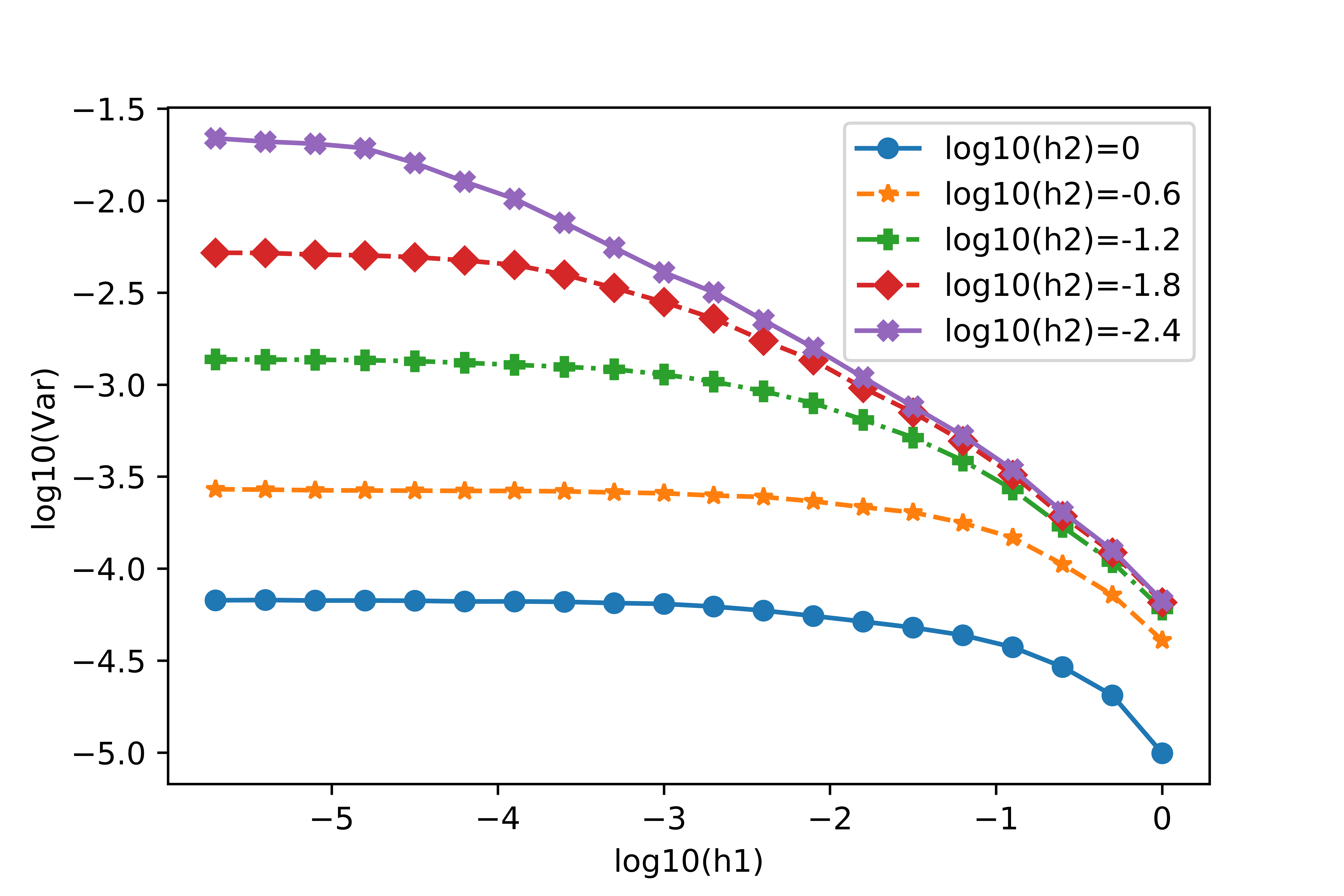
Figure 1. Variance of the estimator

5. Minimax lower bound

In this section, we show that it is impossible to construct any estimator with a uniform rate better (up to a log term) than the rates obtained in Theorems 1–2.

5.1. Lower bounds

For the computation of lower bounds, we introduce the family of S.D.E.

(5.1) $$\text{d}X_{t}=Y_{t}\text{d}t$$

(5.2) $$\text{d}Y_{t}=2\sigma\text{d}B_{t}-[\sigma^{2}\beta(X_{t},Y_{t})Y_{t}+V^{\prime}(X_{t})]\text{d}t,$$

where $\sigma>0$, $\beta$ is a bounded $\mathcal{C}^{1}$ function lower bounded by a strictly positive number and $V$ is $\mathcal{C}^{2}$. As the model satisfies the conditions of HReg we know that the S.D.E. admits a weak solution. We know that if $V$ satisfies HErg then a Lyapounov function exists and the process admits a unique stationary measure, that we note $\pi_{V,\beta}$. In Section 5.2, we make more explicit the connection between $\pi_{V,\beta}$ and the coefficients $V$, $\beta$. Remark that we omit in the notations the dependence on $\sigma$, as $\sigma$ will be fixed in the sequel.

If the stationary measure exists and is unique, we denote $\mathbb{P}_{V,\beta}$ the law of a stationary solution $(X_{t},Y_{t})_{t\geq 0}$ of (5.1)–(5.2). Here, $\mathbb{P}_{V,\beta}$ is a measure on the space of continuous function $\mathcal{C}([0,\infty),\mathbb{R}^{2})$, and we note by $\mathbb{E}_{V,\beta}$ the corresponding expectation. When needed, we will note by $\mathbb{P}_{V,\beta}^{(T)}$ the law of the stationary process $(X_{t},Y_{t})_{t\in[0,T]}$ solution to the S.D.E. (5.1)–(5.2).

In the sequel, we note again $(X,Y)$ the canonical process on $\mathcal{C}([0,\infty),\mathbb{R}^{2})$ or $\mathcal{C}([0,T],\mathbb{R}^{2})$.

In order to write down an expression for the minimax risk of estimation, we have to consider a set of solutions to the S.D.E. (5.1)–(5.2), which are stationary and whose stationary measure has a prescribed Hölder regularity. This leads us to the following definition.

Definition 2.

Let $V:\mathbb{R}\to\mathbb{R}$ be a $\mathcal{C}^{2}$ function satisfying HErg. We consider $k_{1}>0,~{}k_{2}>0,~{}R>0$, and $R^{\prime}>1$ real numbers. We define $\Sigma^{k_{1},k_{2}}(V,R,R^{\prime})$ the set of continuously differentiable functions $\beta:\mathbb{R}^{2}\to\mathbb{R}$ satisfying the following two conditions :

1. $1/R^{\prime}\leq\beta(x,y)\leq R^{\prime}$ for all $(x,y)\in\mathbb{R}^{2}$,

2. the density $\pi_{V,\beta}$ of the stationary measure associated to the S.D.E. (5.1)–(5.2) is such that $\pi_{V,\beta}\in\mathcal{H}^{k_{1},k_{2}}(R)$.

We introduce the minimax risk for the estimation at some point. Let $(x_{0},y_{0})\in\mathbb{R}^{2}$, and $V$, $k_{1},~{}k_{2},~{}R,~{}R^{\prime}$ as in Definition 2. We let

(5.3) $$R_{T}(V,k_{1},k_{2},R,R^{\prime})=\inf_{\widetilde{\pi}_{T}}\sup_{\beta\in\Sigma^{k_{1},k_{2}}(V,R,R^{\prime})}\mathbb{E}_{V,\beta}\left[(\widetilde{\pi}_{T}(x_{0},y_{0})-\pi_{V,\beta}(x_{0},y_{0}))^{2}\right],$$

where the infimum is taken on all possible estimators of $\pi_{T}(x_{0},y_{0})$, that is for $\widetilde{\pi}_{T}=\widetilde{\pi}_{T}(x_{0},y_{0})$ ranging in the set of all the measurable functions of $(X_{t},Y_{t})_{t\in[0,T]}$ with values in $\mathbb{R}$.

Theorem 3.

Let $k_{1},k_{2},R>0$ and assume $y_{0}\neq 0$ and $\max(k_{1},k_{2}/2)>1/2$. Then, there exists $V$ satisfying HErg and $R^{\prime}>1$ such that, for some constant $C>0$, we have :

(5.4) $$R_{T}(V,k_{1},k_{2},R,R^{\prime})\geq CT^{-2v(k_{1},k_{2})},\quad\forall T>1,$$

with

$$v(k_{1},k_{2})=\begin{cases}\frac{k_{2}}{2k_{2}+1},&\text{ if $k_{1}<k_{2}/2$,}\\ \frac{k_{1}}{2k_{1}+1/2},&\text{ if $k_{1}\geq k_{2}/2$.}\end{cases}$$

Remark 4.

1. Theorem 3 tells us that it is impossible to find an estimator with a rate of estimation, for the pointwise $L^{2}$ risk, better than $T^{-v(k_{1},k_{2})}$ on a the class of diffusions $Z=(X,Y)$ having a with $\mathcal{H}^{k_{1},k_{2}}(R)$ stationary measure. On the other hand the estimator introduced in Section 3 achieves this rate, by Theorem 1, for each diffusion $Z=(X,Y)$ satisfying HReg and HErg and with stationary measure in $\mathcal{H}^{k_{1},k_{2}}(R)$.

2. The upper bound given in Theorem 1 is not stated uniformly on the class of all diffusions satisfying HReg and HErg and is not a minimax upper bound. To get uniform upper bound, we would need that the mixing control (2.4) holds uniformly on a class of diffusions whose coefficients satisfy uniform versions of the assumptions HReg, HErg. We are not aware of such uniform mixing results, and hence, getting a uniform version of Theorem 1 is left for further research.

3. The condition $\max(k_{1},k_{2}/2)>1/2$ asserts that $\pi$ is not too irregular with respect to both variables $x$ and $y$. Such assumption is weak, as the stationary measure is typically smoother than the coefficients of the S.D.E. (see point 3 of Remark 5 below).

Theorem 4.

Let $k_{1},k_{2},R>0$ and assume $y_{0}=0$ and $\max(k_{1},k_{2}/3)>2/3$. Then, there exists $V$ satisfying HErg and $R^{\prime}>1$ such that, for some constant $C>0$, we have :

(5.5) $$R_{T}(V,k_{1},k_{2},R,R^{\prime})\geq CT^{-2v^{\prime}(k_{1},k_{2})},\quad\forall T>1,$$

with

$$v^{\prime}(k_{1},k_{2})=\begin{cases}\frac{k_{2}}{2k_{2}+2},&\text{ if $k_{1}<k_{2}/3$,}\\ \frac{k_{1}}{2k_{1}+2/3},&\text{ if $k_{1}\geq k_{2}/3$.}\end{cases}$$

Again, the previous result shows that the estimator introduced in Section 3 is rate efficient, up to a log term, in the case where $y_{0}=0$.

5.2. Explicit link between the drift and the stationary measure

Recall that from Proposition 1, HReg and HErg are sufficient for the existence and uniqueness of a stationary probability of the process solution of (5.1)–(5.2) (see [17] also, or see Talay [15] for related conditions too). In this section, we will characterize explicit relations between $(V,\beta)$ and $\pi_{V,\beta}$.

We need to introduce $A^{\star}_{V,\beta}$ the adjoint on $\mathbf{L}^{2}(\mathbb{R}^{2},\text{d}x\text{d}y)$ of the generator $A_{V,\beta}$ of the process $Z=(X,Y)$ solution to (5.1)–(5.2).

Assume that $V$ is $\mathcal{C}^{2}$ and that $(x,y)\mapsto y\beta(x,y)$ is of class $\mathcal{C}^{1}$. Then we define for $g:\mathbb{R}^{2}\to\mathbb{R}$ any $\mathcal{C}^{2}$ function,

(5.6) $$A^{\star}_{V,\beta}g(x,y)=2\sigma^{2}\frac{\partial^{2}g}{\partial y^{2}}(x,y)-y\frac{\partial g}{\partial x}(x,y)\\ +[\sigma^{2}y\beta(x,y)+V^{\prime}(x)]\frac{\partial g}{\partial y}(x,y)+\sigma^{2}\frac{\partial(y\beta)}{\partial y}(x,y)g(x,y).$$

It can be checked that (5.6) is the expression for the adjoint of the generator of the process. If $g:\mathbb{R}^{2}\to\mathbb{R}$ is a probability density, of class $\mathcal{C}^{2}$, solution to $A^{\star}_{V,\beta}g=0$, then it is an invariant density for the process. Hence, when the stationary distribution $\pi_{V,\beta}$ is unique, it can be computed as solution of the equation $A^{\star}_{V,\beta}\pi_{V,\beta}=0$. From the expression (5.6) it seems impossible to find explicit solutions $g$ to the equation $A^{\star}_{V,\beta}g=0$ for any $V$ and $\beta$, as one need to solve explicitly some P.D.E. Consequently, it seems impossible to write $\pi_{V,\beta}$ as an explicit expression of $(V,\beta)$.

On the other hand, using (5.6) it can be seen that if one consider $g$ and $V$ as fixed and $\beta$ as the unknown variable in the equation $A^{\star}_{V,\beta}g=0$, then finding solution in $\beta$ is simpler as one has to deal with a P.D.E. involving only differentiation with respect to $y$. As a consequence, it will be possible to express $\beta$ as a function of the stationary distribution $\pi$ (for a fixed $V$). This is the object of the next proposition. We need to introduce some notations first.

For $g\in\mathcal{C}^{2}$ and $g>0$, we define for all $(x,y)\in\mathbb{R}^{2}$,

(5.7) $$\xi_{g}(x,y)=\frac{1}{\sigma^{2}g(x,y)}\int_{0}^{y}\big{[}z\frac{\partial g}{\partial x}(x,z)-V^{\prime}(x)\frac{\partial g}{\partial y}(x,z)+2\sigma^{2}\frac{\partial^{2}g}{\partial y^{2}}(x,z)\big{]}\text{d}z,$$

and

(5.8) $$\beta_{g}(x,y)=\begin{cases}\displaystyle\frac{1}{y}\xi_{g}(x,y),\text{ for $y\neq 0$,}\\ \displaystyle\lim_{y\to 0}\frac{1}{y}\xi_{g}(x,y)=\\ \quad\displaystyle\frac{1}{\sigma^{2}g(x,0)}[-V^{\prime}(x)\frac{\partial g}{\partial y}(x,0)+2\sigma^{2}\frac{\partial^{2}g}{\partial y^{2}}(x,0)],\text{ for $y=0$.}\end{cases}$$

Proposition 4.

1. Let $V:\mathbb{R}\to\mathbb{R}$ with regularity $\mathcal{C}^{2}$, $g:\mathbb{R}^{2}\to\mathbb{R}$ with regularity $\mathcal{C}^{2}$ and $g>0$.

   Then, we have that $(x,y)\mapsto y\beta_{g}(x,y)$ is a $\mathcal{C}^{1}$ function and

   (5.9) $$A^{\star}_{V,\beta_{g}}g(x,y)=0,\quad\forall(x,y)\in\mathbb{R}^{2}.$$

   Moreover, $\beta_{g}$ is the unique function solution to (5.9) such that $(x,y)\mapsto y\beta_{g}(x,y)$ is $\mathcal{C}^{0,1}$.

2. Let $V:\mathbb{R}\to\mathbb{R}$ with regularity $\mathcal{C}^{2}$ and satisfying HErg and consider $\pi:\mathbb{R}^{2}\to\mathbb{R}$ a probability density with regularity $\mathcal{C}^{2}$ and $\pi>0$.

   Assume that $1/R^{\prime}<\beta_{\pi}<R^{\prime}$ for some $R^{\prime}>1$, where $\beta_{\pi}$ is defined by (5.8).

   Then, $\pi$ is the unique stationary probability of the S.D.E (5.1)–(5.2) with damping coefficient $\beta=\beta_{\pi}$ and potential $V$

Proof 1) For $g:\mathbb{R}^{2}\to\mathbb{R}$ with regularity $\mathcal{C}^{2}$ and $g>0$ and $\beta$ such that $(x,y)\mapsto y\beta(x,y)$ is of class $\mathcal{C}^{1}$, we can write the equation $A^{\star}_{V,\beta}g(x,y)=0$, recalling (5.6), as

(5.10) $$\frac{\partial(y\beta)}{\partial y}(x,y)+\frac{\frac{\partial g}{\partial y}(x,y)}{g(x,y)}(y\beta(x,y))=i_{g}(x,y)$$

with

$$i_{g}(x,y)=\frac{1}{\sigma^{2}g(x,y)}\left[y\frac{\partial g}{\partial x}(x,y)-V^{\prime}(x)\frac{\partial g}{\partial y}(x,y)-2\sigma^{2}\frac{\partial^{2}g}{\partial y^{2}}(x,y)\right].$$

Let us fix $x\in\mathbb{R}$, we then interpret (5.10) as an ordinary differential equation with differentiation variable $y$, where the unknown parameter is the function $y\mapsto\xi(x,y):=y\beta(x,y)$ :

(5.11) $$\frac{\partial\xi}{\partial y}+\frac{\frac{\partial g}{\partial y}}{g}\xi=i_{g}.$$

A solution of the homogeneous equation $\frac{\partial\xi}{\partial y}+\frac{\frac{\partial g}{\partial y}}{g}\xi=0$ is $\xi(x,y)=1/g(x,y)$. Then, by variation of the constant method, we deduce that the solution to (5.11), has the expression,

$$\xi(x,y)=\frac{1}{g(x,y)}\left[c(x)+\int_{0}^{y}g(x,z)i_{g}(x,z)\text{d}z\right],$$

where $c(x)$ is an integration constant. As $\xi(x,0)=0\times\beta(x,0)=0$, we deduce that $c(x)=0$, $\forall x$. Hence the solution $\xi(x,y)=y\beta(x,y)$ of (5.11) is given by (5.7) and in turn, we deduce that $\beta=\beta_{g}$ given by (5.8) is the unique solution to (5.10) or equivalently to (5.9).

2) Using Ito’s formula, one can check that any $\pi$ solution to $A^{\star}_{V,\beta}\pi=0$ is a stationary measure for the process $(X,Y)$ given by (5.1)–(5.2). From the first part of the proposition, $\pi$ is solution to $A^{\star}_{V,\beta_{\pi}}\pi=0$. By Proposition 1, the stationary measure of the equation with damping coefficient $\beta_{\pi}$ is unique, and is thus equal to $\pi$. $\square$

Remark 5.

1. Is is known that the S.D.E.

   $$\text{d}X_{t}=Y_{t}\text{d}t$$

   $$\text{d}Y_{t}=2\sigma\text{d}B_{t}-[\sigma^{2}\varepsilon Y_{t}+V^{\prime}(X_{t})]\text{d}t.$$

   admits for the stationary measure $\pi(x,y)=C\exp\left(-\frac{\varepsilon}{2}[\frac{y^{2}}{2}+V(x)]\right)$ (see e.g. [5]). As expected, if we take $\pi(x,y)=C\exp\left(-\frac{\varepsilon}{2}[\frac{y^{2}}{2}+V(x)]\right)$ and compute $\beta_{\pi}$ by the formula (5.8), we find $\beta_{\pi}=\varepsilon$.

2. Proposition 4 shows how to compute the damping part of the drift in order to get a diffusion with a prescribed stationary measure. However, it is not clear that for a given $\pi$ the corresponding $\beta_{\pi}$, computed with (5.7)–(5.8) satisfies the sign condition $\beta_{\pi}>1/R^{\prime}$ insuring that the process is indeed ergodic. This is why in part 2) of Proposition 4 we postulate $\beta_{\pi}>1/R^{\prime}$. However, we will see in Section 5.3 that if $\pi$ is a small deviation of $\pi_{0}$ given by $\pi_{0}(x,y)=C\exp\left(-\frac{\varepsilon}{2}[\frac{y^{2}}{2}+V(x)]\right)$, then the corresponding $\beta$ is a small deviation of $\beta_{0}=\varepsilon$ and thus is positive.

3. The equation (5.7) enables to relate the degree of smoothness of the drift coefficient and of the stationary measure, when the latter exists and is unique. Indeed, from (5.7), we get that if $\pi\in\mathcal{C}^{k_{1},k_{2}}$ and $V\in\mathcal{C}^{k_{1}}$, then the associated drift of the S.D.E. $\xi_{\pi}+V^{\prime}$ is $\mathcal{C}^{k_{1}-1,k_{2}-1}$.

5.3. Proof of Theorem 3

The proof of the lower bound is made by a comparison between the minmax risk (5.3) and some Bayesian risk where the Bayesian prior is supported on a set of two elements.

5.3.1. Construction of the prior

Let $k_{1},k_{2}>0$ and $R>0$. We set $V_{0}(x)={\left|x\right|}^{2}$ and define

(5.12) $$\pi_{0}(x,y)=c_{\eta}\exp(-\frac{\eta}{2}[\frac{y^{2}}{2}+x^{2}]),\quad\beta_{0}(x,y)=\eta,\quad\xi_{0}(x,y)=\eta y,$$

where $\eta>0$ and where $c_{\eta}$ is the constant that makes $\pi_{0}$ a probability measure. The function $\pi_{0}$ is $\mathcal{C}^{\infty}$ and it is possible to choose $0<\eta<1/2$ small enough such that

$$\pi_{0}\in\mathcal{H}^{k_{1},k_{2}}(R/2).$$

We know from Section 5.2 that $\pi_{0}$ is the unique stationary measure for $(X^{(0)},Y^{(0)})$ solution of

(5.13) $$\text{d}X^{(0)}_{t}=Y^{(0)}_{t}\text{d}t$$

(5.14) $$\text{d}Y^{(0)}_{t}=2\sigma\text{d}B_{t}-[\sigma^{2}\eta Y^{(0)}_{t}+V_{0}^{\prime}(X^{(0)}_{t})]\text{d}t.$$

Now, if we set ${R^{\prime}=2/\eta>1}$, we have, using $\beta_{0}=\eta$ and recalling Definition 2,

(5.15) $$\beta_{0}\in\Sigma^{k_{1},k_{2}}(V,R/2,R^{\prime}/2).$$

Let $h:\mathbb{R}\to\mathbb{R}$ be a $\mathcal{C}^{\infty}$ function with support on $[-1,1]$ and such that

(5.16) $$h(0)=1,~{}\int_{-1}^{1}h(z)\text{d}z=0,~{}\int_{-1}^{1}zh(z)\text{d}z=0.$$

We set for $T>0$,

(5.17) $$\tilde{\pi}_{T}(x,y)=\pi_{0}(x,y)+\frac{1}{M_{T}}h(\frac{x-x_{0}}{h_{1}(T)})h(\frac{y-y_{0}}{h_{2}(T)}),$$

where $M_{T}$, $h_{1}(T)$, $h_{2}(T)$ will be calibrated later and satisfy

$$M_{T}\xrightarrow{T\to\infty}\infty,~{}h_{1}(T)\xrightarrow{T\to\infty}0,~{}h_{2}(T)\xrightarrow{T\to\infty}0.$$

From (5.16), we see that $\int_{\mathbb{R}^{2}}\tilde{\pi}_{T}(x,y)\text{d}x\text{d}y=\int_{\mathbb{R}^{2}}\pi_{0}(x,y)\text{d}x\text{d}y=1$, and using $\pi_{0}>0$, $1/M_{T}\to 0$ and that $h$ is compactly supported, we see that $\tilde{\pi}_{T}>0$ for $T$ large enough. Hence $\tilde{\pi}_{T}$ is a smooth probability measure for $T$ large enough. We define

$$\tilde{\beta}_{T}(x,y)=\beta_{\tilde{\pi}_{T}}(x,y),\quad\tilde{\xi}_{T}(x,y)=y\tilde{\beta}_{T}(x,y)=\xi_{\tilde{\pi}_{T}}(x,y),$$

where we used the definitions (5.7) and (5.8).

Before proving Theorem 3, we need to state two lemmas. The first lemma shows that the two functions $\beta_{0}$ and $\tilde{\beta}_{T}$ only differ on some vanishing neighbourhood of $(x_{0},y_{0})$.

Lemma 3.

1) Let us define the compact set of $\mathbb{R}^{2}$

$$K_{T}=[x_{0}-h_{1}(T),x_{0}+h_{1}(T)]\times[y_{0}-h_{2}(T),y_{0}+h_{2}(T)].$$

Then, for $T$ large enough, we have for all $(x,y)\notin K_{T}$ :

$$\beta_{0}(x,y)=\tilde{\beta}_{T}(x,y),\quad\xi_{0}(x,y)=\tilde{\xi}_{T}(x,y).$$

2) For $(x,y)\in K_{T}$, we have the control

(5.18) $${\left|\beta_{0}(x,y)-\tilde{\beta}_{T}(x,y)\right|}~\leq\frac{C}{M_{T}}\left[\frac{h_{2}(T)}{h_{1}(T)}+\frac{1}{h_{2}(T)}\right],$$

(5.19) $${\left|\xi_{0}(x,y)-\tilde{\xi}_{T}(x,y)\right|}~\leq\frac{C}{M_{T}}\left[\frac{h_{2}(T)}{h_{1}(T)}+\frac{1}{h_{2}(T)}\right],$$

where $C$ is some constant independent of $T$, $h_{1}(T)$, $h_{2}(T)$, $M_{T}$.

3) We have

$$\int_{\mathbb{R}^{2}}{\left|\tilde{\xi}_{T}(x,y)-\xi_{0}(x,y)\right|}^{2}\text{d}x\text{d}y\leq\frac{C}{M_{T}^{2}}\left[\frac{h_{2}(T)^{3}}{h_{1}(T)}+\frac{h_{1}(T)}{h_{2}(T)}\right].$$

Proof 1) We first prove the $\tilde{\xi}_{T}$ and $\xi_{0}$ coincides on $K_{T}^{c}$. With the definition (5.7) in mind, we set for $g$ of class $\mathcal{C}^{1,2}$:

$$\mathcal{I}[g](x,y) =\frac{1}{\sigma^{2}}\int_{0}^{y}\big{[}z\frac{\partial g}{\partial x}(x,z)-V^{\prime}(x)\frac{\partial g}{\partial y}(x,z)+2\sigma^{2}\frac{\partial^{2}g}{\partial y^{2}}(x,z)\big{]}\text{d}z$$

$$=\mathcal{I}^{1}[g](x,y)+\mathcal{I}^{2}[g](x,y)+\mathcal{I}^{3}[g](x,y),$$

where

(5.20) $$\mathcal{I}^{1}[g](x,y) =\frac{1}{\sigma^{2}}\int_{0}^{y}z\frac{\partial g}{\partial x}(x,z)\text{d}z,$$

(5.21) $$\mathcal{I}^{2}[g](x,y) =-\frac{V^{\prime}(x)}{\sigma^{2}}[g(x,y)-g(x,0)],$$

(5.22) $$\mathcal{I}^{3}[g](x,y) =2~[\frac{\partial g}{\partial y}(x,y)-\frac{\partial g}{\partial y}(x,0)].$$

Using this notation, we have

(5.23) $$\tilde{\xi}_{T}=\frac{1}{\tilde{\pi}_{T}}\mathcal{I}[\tilde{\pi}_{T}],\quad\xi_{0}=\frac{1}{\pi_{0}}\mathcal{I}[\pi_{0}].$$

Let us note

(5.24) $$d_{T}=\tilde{\pi}_{T}-\pi_{0}$$

and by (5.17), we have

(5.25) $$d_{T}(x,y)=\frac{1}{M_{T}}h(\frac{x-x_{0}}{h_{1}(T)})h(\frac{y-y_{0}}{h_{2}(T)}).$$

Since $g\mapsto\mathcal{I}[g]$ is a linear operator we deduce that

(5.26) $$\tilde{\xi}_{T}=\frac{1}{\tilde{\pi}_{T}}\mathcal{I}[\tilde{\pi}_{T}]=\frac{1}{\tilde{\pi}_{T}}\mathcal{I}[\pi_{0}]+\frac{1}{\tilde{\pi}_{T}}\mathcal{I}[d_{T}].$$

If $(x,y)\notin K_{T}$ we have from (5.24), (5.25) and the fact that the support of $h$ is included in $[-1,1]$ that $\tilde{\pi}_{T}(x,y)=\pi_{0}(x,y)$. Thus $\tilde{\xi}_{T}(x,y)=\frac{1}{\pi_{0}(x,y)}\mathcal{I}[\pi_{0}](x,y)+\frac{1}{\pi_{0}(x,y)}\mathcal{I}[d_{T}](x,y)=\xi_{0}(x,y)+\frac{1}{\pi_{0}(x,y)}\mathcal{I}[d_{T}](x,y)$. It follows that the equality of $\tilde{\xi}_{T}$ and $\xi_{0}$ on $K_{T}^{c}$ will a consequence of the following fact:

(5.27) $$\text{for $(x,y)\notin K_{T}$, we have,}\quad\mathcal{I}[d_{T}](x,y)=0.$$

Let us check that (5.27) holds true. To this end, it is enough that $\mathcal{I}^{i}[d_{T}](x,y)=0$ for $i=1,2,3$ and $(x,y)\notin K_{T}$. Since $h$ is a smooth function with compact support on $[-1,1]$, the function $d_{T}$ and its derivatives vanishes outside of the compact set $K_{T}$ by (5.25). Recalling $y_{0}\neq 0$, for $T$ large enough and for all $x\in\mathbb{R}$, the point $(x,0)$ does not belong to $K_{T}$, thus we deduce from (5.21)–(5.22) that $\mathcal{I}^{2}[d_{T}](x,y)=\mathcal{I}^{3}[d_{T}](x,y)=0$ when $(x,y)\notin K_{T}$. It remains to see that $\mathcal{I}^{1}[d_{T}](x,y)=0$ for $(x,y)\notin K_{T}$. We have by (5.20) and (5.25),

(5.28) $$\mathcal{I}^{1}[d_{T}](x,y)=\frac{h^{\prime}((x-x_{0})/h_{1}(T))}{\sigma^{2}M_{T}h_{1}(T)}\int_{0}^{y}zh(\frac{z-y_{0}}{h_{2}(T)})\text{d}z.$$

For $(x,y)\notin K_{T}$, a first possibility is $x\notin[x_{0}-h_{1}(T),x_{0}+h_{1}(T)]$ that leads to $\mathcal{I}^{1}[d_{T}](x,y)=0$ as $h^{\prime}$ vanishes outside $[-1,1]$ and thus $h^{\prime}((x-x_{0})/h_{1}(T))=0$. Otherwise, we must have $y\notin[y_{0}-h_{2}(T),y_{0}+h_{2}(T)]$. For simplicity of the presentation, assume that $y_{0}>0$. Then,

$$\int_{0}^{y}zh(\frac{z-y_{0}}{h_{2}(T)})\text{d}z =\int_{0}^{y}zh(\frac{z-y_{0}}{h_{2}(T)})1_{[y_{0}-h_{2}(T),y_{0}+h_{2}(T)]}(z)\text{d}z,$$

$$=\begin{cases}\displaystyle 0,&\text{ if $y\displaystyle\leq y_{0}-h_{2}(T)$,}\\ \displaystyle\int_{y_{0}-h_{2}(T)}^{y_{0}+h_{2}(T)}zh(\frac{z-y_{0}}{h_{2}(T)})\text{d}z,&\text{ if $\displaystyle y\geq y_{0}+h_{2}(T)$.}\end{cases}$$

But $\int_{y_{0}-h_{2}(T)}^{y_{0}+h_{2}(T)}zh(\frac{z-y_{0}}{h_{2}(T)})\text{d}z=h_{2}(T)\int_{-1}^{1}(y_{0}+h_{2}(T)z)h(z)\text{d}z=0$ using (5.16). This yields to $\mathcal{I}^{1}[d_{T}](x,y)=0$ for $(x,y)\notin K_{T}$ and (5.27) is proved. It follows that $\tilde{\xi}(x,y)=\xi_{0}(x,y)$ for $(x,y)\notin K_{T}$.

The equality between $\tilde{\beta}_{T}$ and $\beta_{0}$ outside $K_{T}$ is a consequence of $\tilde{\beta}_{T}(x,y)=\tilde{\xi}(x,y)/y$, $\beta_{0}(x,y)={\xi_{0}}(x,y)/y$ for $y\neq 0$.

2) We will prove (5.19) first. From (5.23) and (5.26), we have

(5.29) $$\tilde{\xi}_{T}-\xi_{0}=\frac{\pi_{0}-\tilde{\pi}_{T}}{\tilde{\pi}_{T}}\xi_{0}+\frac{1}{\tilde{\pi}_{T}}\mathcal{I}[d_{T}].$$

On the set $K_{T}$, we see that $\tilde{\pi}_{T}=\pi_{0}+d_{T}$ is lower bounded away from $0$ and that $\xi_{0}$ is bounded. Using ${\left\lVert d_{T}\right\rVert}_{\infty}\leq C/M_{T}$ we deduce that

$$\forall(x,y)\in K_{T},~{}{\left|\tilde{\xi}_{T}(x,y)-\xi_{0}(x,y)\right|}\leq C\big{[}\frac{1}{M_{T}}+\mathcal{I}[d_{T}](x,y)\big{]}.$$

Now, ${\left|\mathcal{I}[d_{T}](x,y)\right|}\leq{\left|\mathcal{I}^{1}[d_{T}](x,y)\right|}+{\left|\mathcal{I}^{2}[d_{T}](x,y)\right|}+{\left|\mathcal{I}^{3}[d_{T}](x,y)\right|}$. From (5.21) and (5.25), ${\left|\mathcal{I}^{2}[d_{T}](x,y)\right|}\leq C{\left\lVert d_{T}\right\rVert}_{\infty}\leq C/M_{T}$ and by (5.22), ${\left|\mathcal{I}^{3}[d_{T}](x,y)\right|}\leq C{\left\lVert\frac{\partial d_{T}}{\partial y}\right\rVert}_{\infty}\leq C/(h_{2}(T)M_{T})$. Using (5.28), we have

$${\left|\mathcal{I}^{1}[d_{T}](x,y)\right|}\leq\frac{{\left\lVert h^{\prime}\right\rVert}_{\infty}}{\sigma^{2}M_{T}h_{1}(T)}\int_{y_{0}-h_{2}(T)}^{y_{0}+h_{2}(T)}{\left|z\right|}\text{d}s{\left\lVert h\right\rVert}_{\infty}\leq C\frac{h_{2}(T)}{M_{T}h_{1}(T)}.$$

We deduce that,

$$\forall(x,y)\in K_{T},~{}{\left|\tilde{\xi}_{T}(x,y)-\xi_{0}(x,y)\right|}\leq\frac{C}{M_{T}}\big{[}\frac{h_{2}(T)}{h_{1}(T)}+1+\frac{1}{h_{2}(T)}\big{]},$$

which gives (5.19) as $h_{2}(T)\to 0$.

Eventually, (5.18) follows from the fact that, for $T$ large enough, $K_{T}$ does not intersect the axis $y=0$ since $y_{0}\neq 0$ and the relation between $\tilde{\beta}_{T}(x,y)=\tilde{\xi}(x,y)/y$, $\beta_{0}(x,y)={\xi_{0}}(x,y)/y$.

3) We have,

$$\int_{\mathbb{R}^{2}}{\left|\tilde{\xi}_{T}(x,y)-\xi_{0}(x,y)\right|}^{2}\text{d}x\text{d}y=\int_{K_{T}}{\left|\tilde{\xi}_{T}(x,y)-\xi_{0}(x,y)\right|}^{2}\text{d}x\text{d}y$$

and the third point of the lemma follows from (5.19) with the fact that the Lebesgue measure of $K_{T}$ is proportional to $h_{1}(T)h_{2}(T)$. $\square$

Lemma 4.

Let $\varepsilon>0$ and assume that for all $T$ large,

(5.30) $$M_{T}^{-1}\leq\varepsilon h_{1}(T)^{k_{1}},\quad M_{T}^{-1}\leq\varepsilon h_{2}(T)^{k_{2}},$$

and

$$\frac{h_{2}(T)}{h_{1}(T)}+\frac{1}{h_{2}(T)}=o(M_{T})\text{ as $T\to\infty$.}$$

Then, if $\varepsilon>0$ is small enough, we have

$$\tilde{\beta}_{T}\in\Sigma^{k_{1},k_{2}}(V_{0},R,R^{\prime}),$$

for all $T$ sufficiently large.

Proof From Lemma 3, we know that $\tilde{\beta}_{T}=\beta_{0}$ outside $K_{T}$ and thus is constant equal to $\eta>0$ outside $K_{T}$. For $(x,y)\in K_{T}$, we have by (5.18) in Lemma 3, $\tilde{\beta}_{T}(x,y)=\beta_{0}(x,y)+O\left(\frac{1}{M_{T}}\left[\frac{h_{2}(T)}{h_{1}(T)}+\frac{1}{h_{2}(T)}\right]\right)=\eta+o(1)$. where $C$ is some constant. Thus for $T$ sufficiently large we have

$$\forall(x,y),\quad 1/R^{\prime}=\eta/2<\tilde{\beta}_{T}(x,y)<1<R^{\prime}$$

where we recall that $R^{\prime}=2/\eta>1$. As $V_{0}$ is $\mathcal{C}^{1}$ and satisfy HErg, we can apply the second point of Proposition 4 and deduce that $\tilde{\pi}_{T}$ is the unique stationary measure associated to $\tilde{\beta}_{T}$. Recalling Definition 2, the lemma will be shown as soon as we have,

$$\tilde{\pi}_{T}\in\mathcal{H}^{k_{1},k_{2}}(R).$$

Let us check the Hölder condition with respect to the variable $x$, as the condition with respect to the variable $y$ is similar. For all $(x,y)\in\mathbb{R}^{2}$ and $z\in[-1,1]$,

$${\left|\frac{\partial^{{\lfloor k_{1}\rfloor}}\tilde{\pi}_{T}}{\partial x^{{\lfloor k_{1}\rfloor}}}(x+z,y)-\frac{\partial^{{\lfloor k_{1}\rfloor}}\tilde{\pi}_{T}}{\partial x^{{\lfloor k_{1}\rfloor}}}(x,y)\right|}\leq{\left|\frac{\partial^{{\lfloor k_{1}\rfloor}}\pi_{0}}{\partial x^{{\lfloor k_{1}\rfloor}}}(x+z,y)-\frac{\partial^{{\lfloor k_{1}\rfloor}}\pi_{0}}{\partial x^{{\lfloor k_{1}\rfloor}}}(x,y)\right|}+\\ {\left|\frac{\partial^{{\lfloor k_{1}\rfloor}}d_{T}}{\partial x^{{\lfloor k_{1}\rfloor}}}(x+z,y)-\frac{\partial^{{\lfloor k_{1}\rfloor}}d_{T}}{\partial x^{{\lfloor k_{1}\rfloor}}}(x,y)\right|}\\ \leq\frac{R}{2}{\left|z\right|}^{k_{1}-{\lfloor k_{1}\rfloor}}+{\left|\frac{\partial^{{\lfloor k_{1}\rfloor}}d_{T}}{\partial x^{{\lfloor k_{1}\rfloor}}}(x+z,y)-\frac{\partial^{{\lfloor k_{1}\rfloor}}d_{T}}{\partial x^{{\lfloor k_{1}\rfloor}}}(x,y)\right|}\\ \leq\frac{R}{2}{\left|z\right|}^{k_{1}-{\lfloor k_{1}\rfloor}}+\frac{{\left\lVert h\right\rVert}_{\infty}}{M_{T}h_{1}(T)^{\lfloor k_{1}\rfloor}}{\left|h^{({\lfloor k_{1}\rfloor})}\left(\frac{x+z-x_{0}}{h_{1}(T)}\right)-h^{({\lfloor k_{1}\rfloor})}\left(\frac{x-x_{0}}{h_{1}(T)}\right)\right|}$$

where we have successively used $\tilde{\pi}_{T}=\pi_{0}+d_{T}$, $\pi_{0}\in\mathcal{H}^{k_{1},k_{2}}(R/2)$, and the definition (5.25) of $d_{T}$. We now write

$${\left|h^{({\lfloor k_{1}\rfloor})}\left(\frac{x+z-x_{0}}{h_{1}(T)}\right)-h^{({\lfloor k_{1}\rfloor})}\left(\frac{x-x_{0}}{h_{1}(T)}\right)\right|}\leq\\ {\left|h^{({\lfloor k_{1}\rfloor})}\left(\frac{x+z-x_{0}}{h_{1}(T)}\right)-h^{({\lfloor k_{1}\rfloor})}\left(\frac{x-x_{0}}{h_{1}(T)}\right)\right|}^{k_{1}-{\lfloor k_{1}\rfloor}}*(2{\left\lVert h^{({\lfloor k_{1}\rfloor})}\right\rVert}_{\infty})^{1-(k_{1}-{\lfloor k_{1}\rfloor})}$$

which is smaller than ${\left\lVert h^{({\lfloor k_{1}\rfloor}+1)}\right\rVert}_{\infty}^{k_{1}-{\lfloor k_{1}\rfloor}}{\left|\frac{z}{h_{1}(T)}\right|}^{k_{1}-{\lfloor k_{1}\rfloor}}*(2{\left\lVert h^{({\lfloor k_{1}\rfloor})}\right\rVert}_{\infty})^{1-(k_{1}-{\lfloor k_{1}\rfloor})}$. It implies that

$${\left|\frac{\partial^{{\lfloor k_{1}\rfloor}}\tilde{\pi}_{T}}{\partial x^{{\lfloor k_{1}\rfloor}}}(x+z,y)-\frac{\partial^{({\lfloor k_{1}\rfloor})}\tilde{\pi}_{T}}{\partial x^{{\lfloor k_{1}\rfloor}}}(x,y)\right|}\leq{\left|z\right|}^{k_{1}-{\lfloor k_{1}\rfloor}}\left[\frac{R}{2}+\frac{c_{h}}{M_{T}h_{1}(T)^{k_{1}}}\right]$$

where $c_{h}={\left\lVert h\right\rVert}_{\infty}{\left\lVert h^{({\lfloor k_{1}\rfloor}+1)}\right\rVert}_{\infty}^{k_{1}-{\lfloor k_{1}\rfloor}}(2{\left\lVert h^{({\lfloor k_{1}\rfloor})}\right\rVert}_{\infty})^{1-(k_{1}-{\lfloor k_{1}\rfloor})}$. If one uses (5.30) with any $\varepsilon<\frac{R}{2c_{h}}$, we deduce

$${\left|\frac{\partial^{{\lfloor k_{1}\rfloor}}\tilde{\pi}_{T}}{\partial x^{{\lfloor k_{1}\rfloor}}}(x+z,y)-\frac{\partial^{{\lfloor k_{1}\rfloor}}\tilde{\pi}_{T}}{\partial x^{{\lfloor k_{1}\rfloor}}}(x,y)\right|}\leq R{\left|z\right|}^{k_{1}-{\lfloor k_{1}\rfloor}}.$$

This is the required Hölder control on the derivatives of $\tilde{\pi}_{T}$ with respect to $x$. The lemma follows. $\square$

5.3.2. Proof of the lower bound (5.4) on the minimax risk

Let us recall some notations. We denote $\mathbb{P}_{V,\beta}$ the law of the stationary solution to (5.1)–(5.2) on the canonical space $\mathcal{C}([0,\infty),\mathbb{R}^{2})$ and $\mathbb{E}_{V,\beta}$ the corresponding expectation. We denote by $\mathbb{P}_{V,\beta}^{(T)}$ (resp. $\mathbb{E}_{V,\beta}^{(T)}$) the restrictions of this probability (resp. expectation) on $\mathcal{C}([0,T],\mathbb{R}^{2})$.

Let $\widetilde{\pi}_{T}(x_{0},y_{0})$ be any measurable function from $\mathcal{C}([0,T],\mathbb{R}^{2})$ to $\mathbb{R}$. We will estimate by below, for $T$ large,

$$R(\tilde{\pi}_{T}(x_{0},y_{0})):=\sup_{\beta\in\Sigma^{k_{1},k_{2}}(V_{0},R,R^{\prime})}\mathbb{E}^{(T)}_{V_{0},\beta}\left[(\widetilde{\pi}_{T}(x_{0},y_{0})-\pi_{V_{0},\beta}(x_{0},y_{0}))^{2}\right].$$

Let us assume that the following conditions hold true,

(5.31) $$M_{T}^{-1}\leq\varepsilon h_{1}(T)^{k_{1}},\quad M_{T}^{-1}\leq\varepsilon h_{2}(T)^{k_{2}},$$

(5.32) $$\frac{h_{2}(T)}{h_{1}(T)}+\frac{1}{h_{2}(T)}=o(M_{T})\text{ as $T\to\infty$,}$$

where $\varepsilon$ is sufficiently small to get the conclusion of Lemma 4. We deduce that for $T$ large enough $\tilde{\beta}_{T}\in\Sigma^{k_{1},k_{2}}(V_{0},R,R^{\prime})$. From (5.15), we have $\beta_{0}\in\Sigma^{k_{1},k_{2}}(V_{0},R/2,R^{\prime}/2)\subset\Sigma^{k_{1},k_{2}}(V_{0},R,R^{\prime})$. It follows

$$R(\tilde{\pi}_{T}(x_{0},y_{0}))\geq\frac{1}{2}\mathbb{E}^{(T)}_{V_{0},\tilde{\beta}_{T}}\left[(\widetilde{\pi}_{T}(x_{0},y_{0})-\pi_{V_{0},\tilde{\beta}_{T}}(x_{0},y_{0}))^{2}\right]+\\ \frac{1}{2}\mathbb{E}^{(T)}_{V_{0},\beta_{0}}\left[(\widetilde{\pi}_{T}(x_{0},y_{0})-\pi_{V_{0},\beta_{0}}(x_{0},y_{0}))^{2}\right].$$

Using Lemma 5 below, we know that $Z^{(T)}=\frac{\text{d}\mathbb{P}_{V_{0},\tilde{\beta}_{T}}^{(T)}}{\text{d}\mathbb{P}_{V_{0},\beta_{0}}^{(T)}}$ exists, and we can write

$$R(\tilde{\pi}_{T}(x_{0},y_{0})) \geq\frac{1}{2}\mathbb{E}^{(T)}_{V_{0},\beta_{0}}\left[(\widetilde{\pi}_{T}(x_{0},y_{0})-\pi_{V_{0},\tilde{\beta}_{T}}(x_{0},y_{0}))^{2}Z^{(T)}\right]+$$

$$\quad\quad\quad\quad\quad\quad\quad\frac{1}{2}\mathbb{E}^{(T)}_{V_{0},\beta_{0}}\left[(\widetilde{\pi}_{T}(x_{0},y_{0})-\pi_{V_{0},\beta_{0}}(x_{0},y_{0}))^{2}\right]$$

$$\geq\frac{1}{2\lambda}\mathbb{E}^{(T)}_{V_{0},\beta_{0}}\left[(\widetilde{\pi}_{T}(x_{0},y_{0})-\pi_{V_{0},\tilde{\beta}_{T}}(x_{0},y_{0}))^{2}1_{\{Z^{(T)}\geq\frac{1}{\lambda}\}}\right]+$$

$$\quad\quad\quad\quad\quad\quad\quad\frac{1}{2}\mathbb{E}^{(T)}_{V_{0},\beta_{0}}\left[(\widetilde{\pi}_{T}(x_{0},y_{0})-\pi_{V_{0},\beta_{0}}(x_{0},y_{0}))^{2}1_{\{Z^{(T)}\geq\frac{1}{\lambda}\}}\right]$$

$$=\frac{1}{2\lambda}\mathbb{E}^{(T)}_{V_{0},\beta_{0}} \left[[(\widetilde{\pi}_{T}(x_{0},y_{0})-\pi_{V_{0},\tilde{\beta}_{T}}(x_{0},y_{0}))^{2}+(\widetilde{\pi}_{T}(x_{0},y_{0})-\pi_{V_{0},\beta_{0}}(x_{0},y_{0}))^{2}]1_{\{Z^{(T)}\geq\frac{1}{\lambda}\}}\right]$$

for all $\lambda>1$. As $(\widetilde{\pi}_{T}(x_{0},y_{0})-\pi_{V_{0},\tilde{\beta}_{T}}(x_{0},y_{0}))^{2}+(\widetilde{\pi}_{T}(x_{0},y_{0})-\pi_{V_{0},\beta_{0}}(x_{0},y_{0}))^{2}\geq\left(\frac{\pi_{V_{0},\tilde{\beta}_{T}}(x_{0},y_{0})-\pi_{V_{0},{\beta}_{0}}(x_{0},y_{0})}{2}\right)^{2}$ we deduce,

$$R(\tilde{\pi}_{T}(x_{0},y_{0}))\geq\frac{1}{8\lambda}(\pi_{V_{0},\tilde{\beta}_{T}}(x_{0},y_{0})-\pi_{V_{0},{\beta}_{0}}(x_{0},y_{0}))^{2}\mathbb{P}^{T}_{V_{0},\beta_{0}}\left(Z^{(T)}\geq\frac{1}{\lambda}\right).$$

Since $\pi_{V_{0},\tilde{\beta}_{T}}=\tilde{\pi}_{T}$, $\pi_{V_{0},{\beta}_{0}}=\pi_{0}$ and recalling (5.24), (5.25) with $h(0)=1$ we deduce $\pi_{V_{0},\tilde{\beta}_{T}}(x_{0},y_{0})-\pi_{V_{0},{\beta}_{0}}(x_{0},y_{0})=d_{T}(x_{0},y_{0})=1/M_{T}$, and it follows,

$$R(\tilde{\pi}_{T}(x_{0},y_{0}))\geq\frac{1}{8\lambda}\frac{1}{M_{T}^{2}}\mathbb{P}^{T}_{V_{0},\beta_{0}}\left(Z_{T}\geq\frac{1}{\lambda}\right).$$

From Lemma 5 below we know that $\inf_{T\geq 0}\mathbb{P}^{T}_{V_{0},\beta_{0}}\left(Z_{T}\geq\frac{1}{\lambda}\right)>0$ for some $\lambda=\lambda_{0}$ as soon as

$$\sup_{T\geq 0}T\int_{\mathbb{R}^{2}}{\left|\widetilde{\xi}_{T}(x,y)-\xi_{0}(x,y)\right|}^{2}\text{d}x\text{d}y<\infty.$$

Using the third point of Lemma 3, the latter condition is implied by,

(5.33) $$\sup_{T}\frac{T}{M_{T}^{2}}\left[\frac{h_{2}(T)^{3}}{h_{1}(T)}+\frac{h_{1}(T)}{h_{2}(T)}\right]<\infty.$$

We deduce that

(5.34) $$R(\tilde{\pi}_{T}(x_{0},y_{0}))\geq\frac{C}{M_{T}^{2}},$$

for $C>0$, if the conditions (5.31), (5.32) and (5.33) are satisfied. It remains to find the larger choice for $1/M_{T}^{2}$, subject to the conditions (5.31), (5.32) and (5.33). The optimal choice depends on $k_{1}$ and $k_{2}$.

Case 1, $k_{1}<k_{2}/2$ :

We set $h_{1}(T)=h_{2}(T)^{2}$, and $h_{2}(T)=\left(\frac{1}{\varepsilon M_{T}}\right)^{1/k_{2}}$. The choice for $h_{2}(T)$ saturates one the conditions in (5.31). Let us see that the other condition holds also true . Indeed $1/M_{T}=\varepsilon h_{2}(T)^{k_{2}}=\varepsilon h_{1}(T)^{k_{2}/2}\leq\varepsilon h_{1}(T)^{k_{1}}$ for $T$ large, as $k_{1}<k_{2}/2$ and $h_{1}(T)\to 0$. Thus (5.31) is satisfied.

Plugging the values of $h_{1}(T)$ and $h_{2}(T)$ in (5.33), we obtain the constraint $\frac{T}{M_{T}^{2}}\left(\frac{1}{\varepsilon M_{T}}\right)^{1/k_{2}}\leq C$ for some $C>0$, that leads us to the choice $M_{T}=T^{1/(2+1/k_{2})}=T^{\frac{k_{2}}{2k_{2}+1}}$. Then, the condition (5.32) is satisfied as $k_{2}>1$, indeed $h_{2}(T)/h_{1}(T)+1/h_{2}(T)=2/h_{2}(T)=2\left(\varepsilon M_{T}\right)^{1/k_{2}}=o(M_{T})$.

Eventually, we deduce from the application of (5.34),

(5.35) $$R(\tilde{\pi}_{T}(x_{0},y_{0}))\geq C/M_{T}^{2}=CT^{-\frac{2k_{2}}{2k_{2}+1}}.$$

Case 2, $k_{1}\geq k_{2}/2$ :

We set $h_{1}(T)=h_{2}(T)^{2}$, and $h_{1}(T)=\left(\frac{1}{\varepsilon M_{T}}\right)^{1/k_{1}}$. As $1/M_{T}=\varepsilon h_{1}(T)^{k_{1}}=h_{2}(T)^{2k_{1}}\leq h_{2}(T)^{k_{2}}$, we see that (5.31) is satisfied. Plugging these choices of bandwidths in (5.33), we obtain the constraint $\frac{T}{M_{T}^{2}}\left(\frac{1}{\varepsilon M_{T}}\right)^{1/(2k_{1})}\leq C$ for some $C>0$, that leads us to the choice $M_{T}=T^{1/(2+1/(2k_{1}))}=T^{\frac{k_{1}}{2k_{1}+1/2}}$. Then, the condition (5.32) is satisfied as $k_{1}>1/2$, indeed $h_{2}(T)/h_{1}(T)+1/h_{2}(T)=2/h_{2}(T)=2\left(\varepsilon M_{T}\right)^{1/(2k_{1})}=o(M_{T})$.

Eventually, we deduce from the application of (5.34),

(5.36) $$R(\tilde{\pi}_{T}(x_{0},y_{0}))\geq C/M_{T}^{2}=CT^{-\frac{2k_{1}}{2k_{1}+1/2}}.$$

Gathering (5.35) and (5.36), we have shown Theorem 3. ∎

Lemma 5.

1) The measure $\mathbb{P}^{(T)}_{V_{0},\tilde{\beta}_{T}}$ is absolutely continuous with respect to $\mathbb{P}^{(T)}_{V_{0},\beta_{0}}$.

2) Denote $Z^{(T)}=\frac{\text{d}\mathbb{P}^{(T)}_{V_{0},\tilde{\beta}_{T}}}{\text{d}\mathbb{P}^{(T)}_{V_{0},\beta_{0}}}$ and assume that,

(5.37) $$\sup_{T\geq 0}T\int_{\mathbb{R}^{2}}{\left|\widetilde{\xi}_{T}(x,y)-\xi_{0}(x,y)\right|}^{2}\text{d}x\text{d}y<\infty.$$

Then, there exist $\lambda_{0},~{}C>0$ such that,

$$\mathbb{P}^{(T)}_{V_{0},\beta_{0}}\left(Z^{(T)}\geq\frac{1}{\lambda_{0}}\right)\geq C$$

for all $T$ large enough.

Proof 1) The absolute continuity $\mathbb{P}^{(T)}_{V_{0},\tilde{\beta}_{T}}\ll\mathbb{P}^{(T)}_{V_{0},\beta_{0}}$ and expression for the ratio $Z^{(T)}=\frac{\text{d}\mathbb{P}^{(T)}_{V_{0},\tilde{\beta}_{T}}}{\text{d}\mathbb{P}^{(T)}_{V_{0},\beta_{0}}}$ is obtained by Girsanov formula, changing the drift of the component $Y^{0}$ in (5.14) to the drift appearing in the component $Y^{(T)}$ of the stationary solution of the S.D.E.

$$\text{d}X^{(T)}_{t}=Y^{(T)}_{t}\text{d}t$$

$$\text{d}Y^{(T)}_{t}=2\sigma\text{d}B_{t}-[\sigma^{2}\tilde{\beta}_{T}(Y^{(T)}_{t})Y^{(T)}_{t}+V_{0}^{\prime}(X^{(T)}_{t})]\text{d}t.$$

By classical computations (see Theorem 1.12 in [10]), we have

(5.38) $$Z^{(T)}=\frac{\text{d}\mathbb{P}^{(T)}_{V_{0},\tilde{\beta}_{T}}}{\text{d}\mathbb{P}^{(T)}_{V_{0},\beta_{0}}}\left((X_{s},Y_{s})_{0\leq s\leq T}\right)\\ =\frac{\tilde{\pi}_{T}(X_{0},Y_{0})}{\pi_{0}(X_{0},Y_{0})}\exp\Bigg{\{}-\frac{1}{4}\int_{0}^{T}\Delta_{T}(X_{s},Y_{s})\text{d}Y_{s}\\ -\frac{1}{8\sigma^{2}}\int_{0}^{T}[\sigma^{2}{\xi}_{0}(X_{s},Y_{s})+\sigma^{2}\Delta_{T}(X_{s},Y_{s})+V_{0}^{\prime}(X_{s},Y_{s})]^{2}-[\sigma^{2}{\xi}_{0}(X_{s},Y_{s})+V_{0}^{\prime}(X_{s},Y_{s})]^{2}\text{d}s\Bigg{\}},$$

where $\Delta_{T}(x,y)=\tilde{\xi}_{T}(x,y)-{\xi}_{0}(x,y)=y\tilde{\beta}_{T}(x,y)-y{\beta}_{0}(x,y)$. Let us stress that the ratio $\frac{\tilde{\pi}_{T}(X_{0},Y_{0})}{\pi_{0}(X_{0},Y_{0})}$ in the expression of $Z^{(T)}$ comes from the fact that the two diffusions $(X^{(0)},X^{(0)})_{t}$ and $(X^{(T)},X^{(T)})_{t}$ have different initial laws, since they are both stationary, with the different stationary laws.

2) Let us control by below $\mathbb{P}^{(T)}_{V_{0},\beta_{0}}(Z^{(T)}\geq\frac{1}{\lambda})$ for $\lambda>0$. Recalling the definition of $\pi_{0}$ and $\tilde{\pi}_{T}$ (see (5.12), (5.17))), we see that $\tilde{\pi}_{T}/\pi_{0}$ is equal to $1$ outside some compact set (that can be chosen independent of $T$), and converges uniformly to $1$ on this compact set. Hence it is bounded away from zero if $T$ is large, and $\frac{\tilde{\pi}_{T}(X_{0},Y_{0})}{\pi_{0}(X_{0},Y_{0})}\geq C>0$ almost surely.

Hence, we will focus on the exponential term in (5.38), that we note $\mathcal{E}^{(T)}=Z^{(T)}\frac{\pi_{0}(X_{0},Y_{0})}{\tilde{\pi}_{T}(X_{0},Y_{0})}$. We know that under $\mathbb{P}^{(T)}_{V_{0},\beta_{0}}$ the canonical process $(X,Y)_{t}$ has the same law as $(X^{(0)},Y^{(0)})_{t}$ defined in (5.13)–(5.14). Hence, the law of $\log(\mathcal{E}^{(T)})$ is the law of the random variable

$$-\frac{1}{4}\int_{0}^{T}\Delta_{T}(X^{(0)}_{s},Y^{(0)}_{s})\text{d}Y^{(0)}_{s}\\ -\frac{1}{8\sigma^{2}}\int_{0}^{T}[\sigma^{2}{\xi}_{0}(X^{(0)}_{s},Y^{(0)}_{s})+\sigma^{2}\Delta_{T}(X^{(0)}_{s},Y^{(0)}_{s})+V_{0}^{\prime}(X^{(0)}_{s},Y^{(0)}_{s})]^{2}\\ -[\sigma^{2}{\xi}_{0}(X^{(0)}_{s},Y^{(0)}_{s})+V_{0}^{\prime}(X^{(0)}_{s},Y^{(0)}_{s})]^{2}\text{d}s.$$

This random variable is equal, using (5.14) and after some computations, to

$$-\frac{\sigma}{2}\int_{0}^{T}\Delta_{T}(X^{(0)}_{s},Y^{(0)}_{s})\text{d}B_{s}-\frac{\sigma^{2}}{8}\int_{0}^{T}\Delta_{T}(X^{(0)}_{s},Y^{(0)}_{s})^{2}\text{d}s$$

$$:= -M_{T}-I_{T}.$$

Using the previous considerations we can write that, for $T$ large enough,

$$\mathbb{P}^{(T)}_{V_{0},\beta_{0}}(Z^{(T)}\geq\frac{1}{\lambda}) \geq\mathbb{P}^{(T)}_{V_{0},\beta_{0}}(\mathcal{E}^{(T)}\geq\frac{1}{C\lambda})$$

$$=\mathbb{P}^{(T)}_{V_{0},\beta_{0}}\left(-\log\mathcal{E}^{(T)}\leq\log(C\lambda)\right)$$

$$=1-\mathbb{P}^{(T)}_{V_{0},\beta_{0}}\left(-\log\mathcal{E}^{(T)}>\log(C\lambda)\right)$$

$$\geq 1-\mathbb{P}^{(T)}_{V_{0},\beta_{0}}\left({\left|\log\mathcal{E}^{(T)}\right|}>\log(C\lambda)\right)$$

$$=1-\mathbb{P}\left({\left|M_{T}+I_{T}\right|}>\log(C\lambda)\right)$$

where in the last line we have used that the law of $\log\mathcal{E}^{(T)}$ under $\mathbb{P}^{(T)}_{V_{0},\beta_{0}}$ is the law of $-M_{T}-I_{T}$. Assume now that $\lambda>1/C$, then using Markov inequality, we can write

$$\mathbb{P}\left({\left|M_{T}+I_{T}\right|}>\log(C\lambda)\right) \leq\mathbb{P}\left({\left|M_{T}\right|}>\frac{1}{2}\log(C\lambda)\right)+\mathbb{P}\left({\left|I_{T}\right|}>\frac{1}{2}\log(C\lambda)\right)$$

$$\leq\frac{4}{\log(C\lambda)^{2}}\mathbb{E}(M_{T}^{2})+\frac{2}{\log(C\lambda)}\mathbb{E}({\left|I_{T}\right|})$$

Since $\mathbb{E}(M_{T}^{2})=2\mathbb{E}(I_{T})$ by Ito’s isometry, we see that the condition

(5.39) $$\sup_{T\geq 0}~{}\mathbb{E}(I_{T})<\infty$$

is sufficient to get that there exists $\lambda_{0}$ such that for any $T$ large enough we have,

$$\mathbb{P}^{(T)}_{V_{0},\beta_{0}}(Z^{(T)}\geq\frac{1}{\lambda_{0}})\geq 1/2.$$

It remains to check that (5.39) holds true. Recalling that $I_{T}=\frac{\sigma^{2}}{8}\int_{0}^{T}\Delta_{T}(X_{s}^{(0)},Y_{s}^{(0)})^{2}\text{d}s$ and using that the process $(X^{(0)}_{t},Y^{(0)}_{t})_{t\geq 0}$ is stationary, with invariant law $\pi_{0}$ we have

$$\mathbb{E}(I_{T})=T\frac{\sigma^{2}}{8}\mathbb{E}\big{[}\Delta_{T}(X_{0}^{(0)},Y_{0}^{(0)})^{2}\big{]}=T\frac{\sigma^{2}}{8}\int_{\mathbb{R}^{2}}\Delta_{T}(x,y)^{2}{\pi}_{0}(x,y)\text{d}x\text{d}y.$$

Since $\pi_{0}$ is a bounded function by (5.12), we deduce

$$\mathbb{E}(I_{T})\leq CT\int_{\mathbb{R}^{2}}\Delta_{T}(x,y)^{2}\text{d}x\text{d}y.$$

Recalling that by definition $\Delta_{T}=\tilde{\xi}_{T}-{\xi}_{0}$ and using the assumption (5.37) in the statement of the lemma, we deduce that (5.39) holds true and the lemma follows. $\square$

5.4. Proof of Theorem 4

The scheme of the proof is similar to the proof of Theorem 3. However, one needs some modifications taking into account that $y_{0}=0$.

5.4.1. Constuction of the prior

The prior is the same as in the proof of Theorem 3 except that we need to modify slightly the functions $V_{0}$ and $h$. Let us give more details. Let $k_{1}$, $k_{2}$ and $R>0$. We choose $V_{0}:\mathbb{R}\to\mathbb{R}$ a $\mathcal{C}^{\infty}$ function such that $V_{0}(x)=x^{2}$ for ${\left|x\right|}$ large and $V^{\prime}_{0}(x)=0$ on a neighbourhood of $x_{0}$, and we define

$$\pi_{0}(x,y)=c_{\eta}\exp(-\frac{\eta}{2}[\frac{y^{2}}{2}+V_{0}(x)]),\quad\beta_{0}(x,y)=\eta,\quad\xi_{0}(x,y)=\eta y,$$

where $0<\eta<1/2$ and where $c_{\eta}$ is the constant that make $\pi_{0}$ a probability measure. The function $\pi_{0}$ is $\mathcal{C}^{\infty}$ and it is possible to choose $\eta$ small enough such that

$$\pi_{0}\in\mathcal{H}^{k_{1},k_{2}}(R/2).$$

We know from Section 5.2 that $\pi_{0}$ is the unique stationary measure of the process $(X^{(0)},Y^{(0)})$ solution to the stochastic differential equation (5.13)–(5.14). If we set $R^{\prime}=2/\eta$, then recalling Definition 2 we have $\beta_{0}\in\Sigma^{k_{1},k_{2}}(V,R/2,R^{\prime}/2)$.

Let $h:\mathbb{R}\to\mathbb{R}$ be a $\mathcal{C}^{\infty}$ function with support on $[-1,1]$ such that,

(5.40) $$h(0)=1,~{}h^{\prime}(0)=0,~{}\int_{-1}^{1}h(z)\text{d}z=0,~{}\int_{0}^{1}zh(z)\text{d}z=\int_{-1}^{0}zh(z)\text{d}z=0.$$

For $T>0$ we define the perturbation of $\pi_{0}$, as in Section 5.3.1 by

$$\tilde{\pi}_{T}(x,y)=\pi_{0}(x,y)+\frac{1}{M_{T}}h(\frac{x-x_{0}}{h_{1}(T)})h(\frac{y}{h_{2}(T)}),$$

where $M_{T}\to\infty$, $h_{1}(T)\to 0$, $h_{2}(T)\to 0$ will be calibrated latter. Again $\tilde{\pi}_{T}$ is a smooth probability measure for $T$ large enough and we define

$$\tilde{\beta}_{T}(x,y)=\beta_{\tilde{\pi}_{T}}(x,y),\quad\tilde{\xi}_{T}(x,y)=y\tilde{\beta}_{T}(x,y)=\xi_{\tilde{\pi}_{T}}(x,y),$$

where we used the definitions (5.7) and (5.8).

The following lemma gives an assessment of the difference between $\beta_{0}$ and $\tilde{\beta}_{T}$.

Lemma 6.

1) Recall the definition of the following compact set of $\mathbb{R}^{2}$

$$K_{T}=[x_{0}-h_{1}(T),x_{0}+h_{1}(T)]\times[-h_{2}(T),h_{2}(T)].$$

Then, for $T$ large enough, we have for all $(x,y)\notin K_{T}$ :

$$\beta_{0}(x,y)=\tilde{\beta}_{T}(x,y),\quad\xi_{0}(x,y)=\tilde{\xi}_{T}(x,y).$$

2) For $(x,y)\in K_{T}$, we have the control,

(5.41) $${\left|\beta_{0}(x,y)-\tilde{\beta}_{T}(x,y)\right|}~\leq\frac{C}{M_{T}}\left[\frac{h_{2}(T)}{h_{1}(T)}+\frac{1}{h_{2}(T)^{2}}\right],$$

(5.42) $${\left|\xi_{0}(x,y)-\tilde{\xi}_{T}(x,y)\right|}~\leq\frac{C}{M_{T}}\left[\frac{h_{2}(T)^{2}}{h_{1}(T)}+\frac{1}{h_{2}(T)}\right],$$

where $C$ is some constant independent of $T$, $h_{1}(T)$, $h_{2}(T)$, $M_{T}$.

3) We have

$$\int_{\mathbb{R}^{2}}{\left|\tilde{\xi}_{T}(x,y)-\xi_{0}(x,y)\right|}^{2}\text{d}x\text{d}y\leq\frac{C}{M_{T}^{2}}\left[\frac{h_{2}(T)^{5}}{h_{1}(T)}+\frac{h_{1}(T)}{h_{2}(T)}\right].$$

Proof 1) We first prove that $\tilde{\xi}_{T}$ and $\xi_{0}$ coincides on $K_{T}^{c}$. Using the notations and arguments of Lemma 3, we know that $\tilde{\xi}_{T}(x,y)=\xi_{0}(x,y),$ for all $(x,y)\notin K_{T}$ is a consequence of $\mathcal{I}[d_{T}](x,y)=0$ for $(x,y)\notin K_{T}$. We recall that $\mathcal{I}=\sum_{i=1}^{3}\mathcal{I}^{i}$ is given by (5.20)–(5.22) and $d_{T}(x,y)=\tilde{\pi}_{T}(x,y)-\pi_{0}(x,y)$ is given by :

(5.43) $$d_{T}(x,y)=\frac{1}{M_{T}}h(\frac{x-x_{0}}{h_{1}(T)})h(\frac{y}{h_{2}(T)}).$$

If $(x,y)\notin K_{T}$, the first situation is ${\left|x-x_{0}\right|}>h_{1}(T)$, then $d_{T}(x,z)=\frac{\partial d_{T}}{\partial x}(x,z)=\frac{\partial d_{T}}{\partial y}(x,z)=0$ for all $z\in\mathbb{R}$ and we deduce that $\mathcal{I}^{i}[d_{T}](x,y)=0$ for $i=1,2,3$. The second situation is ${\left|y\right|}>h_{2}(T)$ and ${\left|x-x_{0}\right|}\leq h_{1}(T)$. In that case $\mathcal{I}^{2}[d_{T}](x,y)=0$ for $T$ large enough, by using that from assumption on $V_{0}$, $V^{\prime}_{0}(x)=0$ for $x$ in some neighbourhood of $x_{0}$. From (5.22), we have $\mathcal{I}^{3}[d_{T}](x,y)=\frac{2}{M_{T}h_{2}(T)}h(\frac{x-x_{0}}{h_{1}(T)})[h^{\prime}(\frac{y}{h_{2}(T)})-h^{\prime}(0)]$ which is equal to $0$ since ${\left|y\right|}>h_{2}(T)$ and $h^{\prime}(0)=0$ by (5.40). In order to check that $\mathcal{I}^{1}[d_{T}](x,y)=0$, let us assume for simplicity that $y>h_{2}(T)$, as the case $y<-h_{2}(T)$ is similar. Then,

$$\mathcal{I}^{1}[d_{T}](x,y)=\frac{1}{\sigma^{2}h_{1}(T)}\int_{0}^{h_{2}}zh(\frac{z}{h_{2}(T)})\text{d}zh^{\prime}(\frac{x-x_{0}}{h_{1}(T)})\\ =\frac{h_{2}(T)^{2}}{\sigma^{2}h_{1}(T)}\int_{0}^{1}zh(z)\text{d}zh^{\prime}(\frac{x-x_{0}}{h_{1}(T)})=0$$

by (5.40). Eventually, this gives that $\mathcal{I}[d_{T}](x,y)=0$ for $(x,y)\notin K_{T}$, and thus $\tilde{\xi}_{T}(x,y)=\xi_{0}(x,y)$.

The equality between the functions $\tilde{\beta}_{T}$ and $\beta_{0}$ on $K_{T}^{c}$ is a consequence of $\tilde{\beta}_{T}(x,y)=\tilde{\xi}(x,y)/y$, $\beta_{0}(x,y)={\xi_{0}}(x,y)/y$ for $y\neq 0$.

2) We first prove (5.42). Recalling (5.29), the fact that ${\left\lVert\pi_{0}-\tilde{\pi}\right\rVert}_{\infty}={\left\lVert d_{T}\right\rVert}_{\infty}\leq C/M_{T}$, and that $\tilde{\pi}_{T}$ is lower bounded on $K_{T}$ as soon as $T$ is large enough, we deduce

$$\forall(x,y)\in K_{T},~{}{\left|\tilde{\xi}_{T}(x,y)-\xi_{0}(x,y)\right|} \leq C\big{[}\frac{{\left|\xi_{0}(x,y)\right|}}{M_{T}}+\mathcal{I}[d_{T}](x,y)\big{]}$$

(5.44) $$\leq C\big{[}\frac{{\left|y\right|}}{M_{T}}+\mathcal{I}[d_{T}](x,y)\big{]}.$$

Now, we use ${\left|\mathcal{I}[d_{T}](x,y)\right|}\leq{\left|\mathcal{I}^{1}[d_{T}](x,y)\right|}+{\left|\mathcal{I}^{2}[d_{T}](x,y)\right|}+{\left|\mathcal{I}^{3}[d_{T}](x,y)\right|}$. From (5.20), we have ${\left|\mathcal{I}^{1}[d_{T}](x,y)\right|}\leq C{\left|\int_{0}^{y}z\text{d}z\right|}{\left\lVert\frac{\partial d_{T}}{\partial x}\right\rVert}_{\infty}\leq C{\left|y\right|}h_{2}(T)\frac{C}{M_{T}h_{1}(T)}$, for all $(x,y)\in K_{T}=[x_{0}-h_{1}(T),x_{0}+h_{1}(T)]\times[-h_{2}(T),h_{2}(T)]$, and where we have used the expression (5.43) for $d_{T}$. As $x\mapsto V^{\prime}(x)$ vanishes on a neighbourhood of $x_{0}$, we get that for $T$ large enough $\mathcal{I}^{2}[d_{T}](x,y)=0$ for $(x,y)\in K_{T}$. From (5.22), we deduce ${\left|\mathcal{I}^{3}[d_{T}](x,y)\right|}\leq C{\left|y\right|}{\left\lVert\frac{\partial^{2}d_{T}}{\partial y^{2}}\right\rVert}_{\infty}\leq C\frac{{\left|y\right|}}{M_{T}h_{2}(T)^{2}}$. Collecting the controls on $\mathcal{I}^{i}[d_{T}](x,y)$ for $i=1,2,3$, with (5.44) we get

$$\forall(x,y)\in K_{T},~{}{\left|\tilde{\xi}_{T}(x,y)-\xi_{0}(x,y)\right|}\leq C\frac{{\left|y\right|}}{M_{T}}\big{[}1+\frac{h_{2}(T)}{h_{1}(T)}+\frac{1}{h_{2}(T)^{2}}\big{]}.$$

Using that for $(x,y)\in K_{T}$, we have ${\left|y\right|}\leq h_{2}(T)$ and the last equation implies (5.42). Moreover, from the fact that $\tilde{\xi}_{T}(x,y)-\xi_{0}(x,y)=y[\tilde{\beta}_{T}(x,y)-\beta_{0}(x,y)]$, it implies (5.41).

3) The third point of the lemma in a consequence of the first two points and the fact that the Lebesgue measure of $K_{T}$ is proportional to $h_{1}(T)h_{2}(T)$. $\square$

We now state a result analogous to Lemma 4, but in the situation $y_{0}=0$.

Lemma 7.

Let $\varepsilon>0$ and assume that for all $T$ large,

$$M_{T}^{-1}\leq\varepsilon h_{1}(T)^{k_{1}},\quad M_{T}^{-1}\leq\varepsilon h_{2}(T)^{k_{2}},$$

and

$$\frac{h_{2}(T)}{h_{1}(T)}+\frac{1}{h_{2}(T)^{2}}=o(M_{T})\text{ as $T\to\infty$.}$$

Then, if $\varepsilon>0$ is small enough, we have

$$\tilde{\beta}_{T}\in\Sigma^{k_{1},k_{2}}(V_{0},R,R^{\prime}),$$

for all $T$ sufficiently large.

We omit the proof of Lemma 7 as it is similar to the proof of Lemma 4 (except that we use (5.41) instead of (5.18)).

5.4.2. Proof of the lower bound (5.5) on the minimax risk

We omit most of the details of the proof as it is very similar to the proof given in Section 5.3.2. Indeed, by repeating the arguments of the proof given in Section 5.3.2, relying on Lemmas 6–7 instead of Lemmas 3–4, we deduce that,

(5.45) $$R(\widetilde{\pi}_{T}(x_{0},0))\geq\frac{C}{M_{T}^{2}},$$

as soon as we can find $\varepsilon>0$, $h_{1}(T)\to 0$, $h_{2}(T)\to 0$ and $M_{T}\to\infty$ satisfying the conditions

(5.46) $$M_{T}^{-1}\leq\varepsilon h_{1}(T)^{k_{1}},\quad M_{T}^{-1}\leq\varepsilon h_{2}(T)^{k_{2}},$$

(5.47) $$\frac{h_{2}(T)}{h_{1}(T)}+\frac{1}{h_{2}(T)^{2}}=o(M_{T})\text{ as $T\to\infty$},$$

(5.48) $$\sup_{T}\frac{T}{M_{T}^{2}}\left[\frac{h_{2}(T)^{5}}{h_{1}(T)}+\frac{h_{1}(T)}{h_{2}(T)}\right]<\infty.$$

Let us maximise $1/M_{T}^{2}$ under these three constraints.

Case 1, $k_{1}<k_{2}/3$ : we set $h_{1}(T)=h_{2}(T)^{3}$ and $h_{2}(T)=\left(\frac{1}{\varepsilon M_{T}}\right)^{1/k_{2}}$ and the conditions (5.46) hold true, using $k_{1}<k_{2}/3$. With these choices, the condition (5.48) reduces to the boundedness of $\frac{T}{M_{T}^{2}}M_{T}^{-2/k_{2}}$, which is implied if we set $M_{T}=T^{-\frac{k_{2}}{2+2k_{2}}}$. Next (5.47) holds true as $\frac{h_{2}(T)}{h_{1}(T)}+\frac{1}{h_{2}(T)^{2}}=O(\frac{1}{h_{2}(T)^{2}})=O(M_{T}^{2/k_{2}})=o(M_{T})$ as $k_{2}>2$. Hence, we can use (5.45) with $M_{T}=T^{-\frac{1}{2+2k_{2}}}$, yielding to (5.5) in the case $k_{1}<k_{2}/3$.

Case 2, $k_{1}\geq k_{2}/3$ : we set $h_{1}(T)=h_{2}(T)^{3}$ and $h_{1}(T)=\left(\frac{1}{\varepsilon M_{T}}\right)^{1/k_{1}}$ and the conditions (5.46) follows. Now, the condition (5.48) reduces to the boundedness of $\frac{T}{M_{T}^{2}}M_{T}^{-2/(3k_{1})}$, which yields to the choice $M_{T}=T^{-\frac{k_{1}}{2k_{1}+2/3}}$. Next (5.47) holds true as $\frac{h_{2}(T)}{h_{1}(T)}+\frac{1}{h_{2}(T)^{2}}=O(\frac{1}{h_{2}(T)^{2}})=O(M_{T}^{2/(3k_{1})})=o(M_{T})$ as $k_{1}>2/3$. Eventually, we deduce (5.5) from (5.45).

6. Appendix

In this section we prove the technical Lemmas 1–2 on the semi group of the process.

6.1. Proof of Lemma 1

This proof is exactly the same as the one of Corollary 2.12 in [1], after remarking that the results of Theorem 2.1. in [9] can be applied to S.D.E. with $\mathcal{C}^{1}$ coefficients. ∎

6.2. Proof of Lemma 2

We first prove that (4.4) holds for $t=D$. Let us denote $\widetilde{K}=\{z\in\mathbb{R}^{2}\mid d(z,K)\leq 1\}$ the compact set of points at distance less than $1$ of $K$. Since $D<1$, we can apply Lemma 1 with the choice of compact set $\widetilde{K}$, to get that if $f$ has support on $K\subset\widetilde{K}$, and $z\in\widetilde{K}$

$${\left|P_{D}(f)(z)\right|} \leq\int_{\mathbb{R}^{2}}{\left|f(z^{\prime})\right|}p_{D}(z;z^{\prime})dz^{\prime}$$

$$\leq\int_{\mathbb{R}^{2}}{\left|f(z^{\prime})\right|}p_{D}^{G}(z;z^{\prime})dz^{\prime}+\int_{\mathbb{R}^{2}}{\left|f(z^{\prime})\right|}p_{D}^{U}(z;z^{\prime})dz^{\prime}$$

(6.1) $$\leq\frac{C_{G}}{D^{2}}\int_{\mathbb{R}^{2}}{\left|f(z^{\prime})\right|}dz^{\prime}+C_{U}{\left\lVert f\right\rVert}_{\infty}e^{-1/(C_{U}D)}.$$

Hence, it proves (4.4) for $t=D$ and $z\in\widetilde{K}$.

If $z\notin\widetilde{K}$, we let $T_{\widetilde{K}}=\inf\{t\geq 0\mid Z_{t}\in\widetilde{K}\}$ the entrance time in the compact set $\widetilde{K}$, which is a stopping time. As the support of $f$ is included in $K$, we have by continuity of the process, $P_{D}(f)(z)=E_{z}[f(Z_{D})]=E_{z}[f(Z_{D})1_{\{T_{\widetilde{K}}\leq t\}}]$. Using the strong Markov property at the time $T_{\widetilde{K}}$ we deduce,

(6.2) $$P_{D}(f)(z)=E_{z}[P_{D-T_{\widetilde{K}}}(f)(Z_{T_{\widetilde{K}}})1_{\{T_{\widetilde{K}}\leq D\}}].$$

By the continuity of the process, we remark that $d(Z_{T_{\widetilde{K}}},K)=1$ on the set $T_{\widetilde{K}}\leq D$, and $D-T_{\widetilde{K}}$ in $(0,D)$ as $z\notin\widetilde{K}$. This lead us to consider for $z^{\prime}\in\widetilde{K}$ with $d(z^{\prime},K)=1$ and $s\in(0,D)\subset(0,1)$, an upper bound for

$${\left|P_{s}(f)(z^{\prime})\right|} \leq\int_{\mathbb{R}^{2}}{\left|f(w)\right|}p_{s}^{G}(z^{\prime};w)dw+\int_{\mathbb{R}^{2}}{\left|f(w)\right|}p_{s}^{U}(z^{\prime};w)dw$$

(6.3) $$\leq\int_{\mathbb{R}^{2}}{\left|f(w)\right|}dw\tilde{C}_{G}+C_{U}{\left\lVert f\right\rVert}_{\infty}e^{-1/(C_{U}s)},$$

where $\tilde{C}_{G}=\sup\{p_{s}^{G}(z^{\prime},w)\mid s\in(0,1),w\in K,z^{\prime}\in\widetilde{K}\text{ with }d(z^{\prime},K)=1\}$, and where we used again Lemma 1. We can see that $\tilde{C}_{G}$ is finite. Indeed, if $z^{\prime}=(x^{\prime},y^{\prime})$ is such that $d(z^{\prime},K)=1$ and $w=(w_{1},w_{2})\in K$, we have $p_{s}^{G}(z^{\prime},w)\leq\frac{C_{G}}{s^{2}}\exp(-\frac{1}{C_{G}}[\frac{(w_{2}-y^{\prime})^{2}}{s}+\frac{(w_{1}-x^{\prime}-\frac{w_{2}+y^{\prime}}{2}s)^{2}}{s^{3}}])$. Using the inequality $A^{2}\leq(A-B)^{2}(1+1/s)+B^{2}(1+s)$ for any $A$, $B$, that entails $(A-B)^{2}\geq A^{2}\frac{s}{s+1}-B^{2}s$, we deduce $\frac{(w_{2}-y^{\prime})^{2}}{s}+\frac{(w_{1}-x^{\prime}-\frac{w_{2}+y^{\prime}}{2}s)^{2}}{s^{3}}\geq\frac{(w_{2}-y^{\prime})^{2}}{s}+\frac{(w_{1}-x^{\prime})^{2}}{s^{3}}\frac{s}{s+1}-\frac{(w_{2}+y^{\prime})^{2}}{2s}s$. Using that $s<1$ and that ${\left|w_{2}\right|}$ and ${\left|y^{\prime}\right|}$ are bounded by some constant depending on the compact $K$, we deduce $\frac{(w_{2}-y^{\prime})^{2}}{s}+\frac{(w_{1}-x^{\prime}-\frac{w_{2}+y^{\prime}}{2}s)^{2}}{s^{3}}\geq d(z^{\prime},w)^{2}/(2s)-\tilde{C}_{K}$ for some constant $\tilde{C}_{K}$ depending on the compact $K$ only. It gives $p_{s}^{G}(z^{\prime},w)\leq\frac{C_{G}}{s^{2}}\exp(-\frac{d(z^{\prime},w)^{2}}{C_{G}2s})\exp(\frac{\widetilde{C}_{K}}{C_{G}})$. As $w\in K$ and $d(w^{\prime},K)=1$, we deduce that $p_{s}^{G}(z^{\prime},w)\leq\frac{C_{G}}{s^{2}}\exp(-\frac{1}{C_{G}2s})\exp(\frac{\widetilde{C}_{K}}{C_{G}})$ and thus $\widetilde{C}_{G}$ is finite. Joining (6.3) and (6.2), we deduce that, for $z\notin\widetilde{K}$

$${\left|P_{D}(f)(z)\right|} \leq\widetilde{C}_{G}{\left\lVert f\right\rVert}_{L^{1}(\mathbb{R}^{2})}+C_{U}{\left\lVert f\right\rVert}_{\infty}E_{z}[e^{-1/(C_{U}(D-T_{\widetilde{K}}))}1_{\{T_{\widetilde{K}}\leq D\}}]$$

(6.4) $$\leq\widetilde{C}_{G}{\left\lVert f\right\rVert}_{L^{1}(\mathbb{R}^{2})}+C_{U}{\left\lVert f\right\rVert}_{\infty}e^{-1/(C_{U}D)}.$$

The control (4.4) for $t=D$ is now a consequence of (6.1) and (6.4). Eventually, we prove that (4.4) for $t=D$ is sufficient to deduce the lemma. Let $0<D<1$ and $t>D$, then for $z\in\mathbb{R}^{2}$, we write

$${\left|P_{t}(f)(z)\right|}\leq\int_{\mathbb{R}^{2}}p_{t-D}(z,z^{\prime}){\left|P_{D}(f)(z^{\prime})\right|}dz^{\prime}$$

and using the estimate (4.4) for ${\left|P_{D}(f)(z^{\prime})\right|}$ gives the result for ${\left|P_{t}(f)(z)\right|}$. ∎

References

- [1] Cattiaux P., León, J. and Prieur, C. Estimation for stochastic damping Hamiltonian systems under partial observation I. Invariant density. Stochastic Process. Appl., 124, no. 3, (2014), 1236–1260.
- [2] Comte, F. and Lacour, C. Anisotropic adaptive kernel deconvolution. Annales de l’Institut Henri Poincaré - Probabilités et Statistiques, Vol. 49, No. 2, (2013), 569–609.
- [3] Comte F, and Merlevède, F. Adaptive estimation of the stationary density of discrete and continuous time mixing processes. ESAIM Probab. Statist., 6:211–238, 2002. New directions in time series analysis (Luminy, 2001).
- [4] Comte, F. and Merlevède, F. Super optimal rates for nonparametric density estimation via projection estimators. Stochastic Process. Appl., 115(5):797–826, 2005.
- [5] Comte, F., Prieur, C. and Samson, A. Adaptive estimation for stochastic damping Hamiltonian systems under partial observation. Stochastic Process. Appl. 127 (2017), no. 11, 3689–3718.
- [6] Dalalyan, A. and Reiß, M. Asymptotic statistical equivalence for ergodic diffusions : the multidimensional case Probab. Theory. Relat. Fields, 137(1), 25–47
- [7] Ditlevsen, S. and Sørensen, M. Inference for Observations of Integrated Diffusion Processes. Scandinavian Journal of Statistics, 31 (2004), 417–429. doi:10.1111/j.1467-9469.2004.02_023.x
- [8] Ditlevsen, S. and Samson, A. Hypoelliptic diffusions: discretization, filtering and inference from complete and partial observations, J Royal Statistical Society B, 81, (2019) 361–384.
- [9] Konakov, V., Menozzi, S. and Molchanov, S. Explicit parametrix and local limit theorems for some degenerate diffusion processes, Annales de l’Institut Henri Poincaré - Probabilités et Statistiques, Vol. 46, No. 4, (2010), 908–923.
- [10] Kutoyants, Y. Statistical inference for ergodic diffusion processes. Springer Series in Statistics. Springer-Verlag London, Ltd., London, 2004. xiv+481 pp. ISBN: 1-85233-759-1.
- [11] Leòn, J.R. and Samson, A. Hypoelliptic stochastic FitzHugh-Nagumo neuronal model: mixing, up-crossing and estimation of the spike rate, Annals of Applied Probability, 28, (2018), 2243–2274, .
- [12] Nishiyama, Y. Estimation for the invariant law of an ergodic diffusion process based on high-frequency data, Journal of Nonparametric Statistics, 23:4, 909-915, DOI: 10.1080/10485252.2011.591397
- [13] Nguyen, H-T. Density estimation in a continuous-time stationary Markov process. Ann. Statist., 7(2):341–348, 1979.
- [14] Strauch, C. Adaptive invariant density estimation for ergodic diffusions over anisotropic classes. Ann. Statist., 46(6B):3451–3480, 2018.
- [15] Talay, D. Stochastic Hamiltonian Systems: Exponential Convergence to the Invariant Measure, and Discretization by the Implicit Euler Scheme, Markov Processes Relat. Fields, 8, (2002), 1–36.
- [16] Tsybakov, A. Introduction to nonparametric estimation. Revised and extended from the 2004 French original. Translated by Vladimir Zaiats. Springer Series in Statistics. Springer, New York, 2009. xii+214 pp. ISBN: 978-0-387-79051-0.
- [17] Wu, L. Large and moderate deviations and exponential convergence for stochastic damping Hamiltonian systems, Stochastic Processes and their Applications, 91, (2001), 205–238.