Global Sensitivity Analysis on Numerical Solver Parameters of Particle-In-Cell Models in Particle Accelerator Systems

Abstract

Every computer model depends on numerical input parameters that are chosen according to mostly conservative but rigorous numerical or empirical estimates. These parameters could for example be the step size for time integrators, a seed for pseudo-random number generators, a threshold or the number of grid points to discretize a computational domain. In case a numerical model is enhanced with new algorithms and modelling techniques the numerical influence on the quantities of interest, the running time as well as the accuracy is often initially unknown.
Usually parameters are chosen on a trial-and-error basis neglecting the computational cost versus accuracy aspects. As a consequence the cost per simulation might be unnecessarily high which wastes computing resources. Hence, it is essential to identify the most critical numerical parameters and to analyze systematically their effect on the result in order to minimize the time-to-solution without losing significantly on accuracy. Relevant parameters are identified by global sensitivity studies where Sobol’ indices are common measures. These sensitivities are obtained by surrogate models based on polynomial chaos expansion.
In this paper, we first introduce the general methods for uncertainty quantification. We then demonstrate their use on numerical solver parameters to reduce the computational costs and discuss further model improvements based on the sensitivity analysis. The sensitivities are evaluated for neighbouring bunch simulations of the existing PSI Injector II and PSI Ring as well as the proposed DAE$\delta$ALUS Injector cyclotron and simulations of the rf electron gun of the Argonne Wakefield Accelerator.

1 Introduction

Numerical models in scientific research disciplines are usually extremely complex and computationally intensive. A common feature to all is the dependency on numerical model parameters that do not represent an actual property of the underlying scientific problem. They are either prescribed in the source code and, thus, hidden to the user or can be chosen at runtime. Examples are the seed for pseudo random number generators, an error threshold in a convergence criterion, the number of grid points in mesh-based models or the step size in time integrators. Latter two are often chosen to satisfy memory constraints or time limits. When applying new algorithms and modelling techniques the sensitivity of such input values on the response is usually studied by varying only a single parameter. While this captures the main influence of the tested parameter, possible correlations with other parameters are missed. A remedy is the evaluation of Sobol’ indices [1] which are variance-based global sensitivity measures to express both individual and correlated parameter influences. Instead of Monte Carlo estimates, these quantifiers can easily be obtained by surrogate models based on polynomial chaos expansion (PCE). Uncertainty quantification (UQ) based on PCE is generally used in many areas of scientific computing and modelling [2, 3, 4, 5] and several frameworks exist such as [6, 7, 8]. The coefficients of the truncated PCE that are required to determine Sobol’ indices are mostly computed using the projection or regression method [9]. Since some numerical parameters are limited to integers, the former method is not applicable.

In this paper we study the sensitivity of adaptive mesh refinement (AMR) and multi bunch [10, 11] parameters in Particle-In-Cell (PIC) simulations of high intensity cyclotrons where we use the new AMR capabilities of OPAL (Object Oriented Parallel Accelerator Library) [12] as presented in [13]. We further explore the sensitivity of a rf electron gun model with respect to the number of macro particles, the energy binning and the time step. The sensivitities are evaluated using ordinary least squares and Bayesian compressive sensing (BCS) [14, 15]. Both methods are part of the uncertainty quantification toolkit UQTk [16, 17] (version 3.0.4). The results are cross-checked using Chaospy [7] (version 3.0.5) together with the orthogonal matching pursuit [18, 19] regression model of the Python machine learning library scikit-learn [20, 21] (version 0.21.2).

Although we apply UQ on numerical solver parameters, it is a general method used for example in [5] to evaluate the sensitivities and to predict the quantities of interest due to uncertainties in physical parameters.

The paper is organised as follows: In Sec. 2.1 we elaborate the physical applications and their numerical modelling. An introduction to UQ is given in Sec. 3. The experimental setup and its results are presented in Sec. 4 and Sec. 5, respectively. In Sec. 6 are the final conclusions.

2 Applications

2.1 High Intensity Cyclotrons

Cyclotrons are circular machines that accelerate charged particles (e.g. protons) or ions (e.g. $H_{2}^{+}$). Depending on the particle species and delivered energy, these machines find different applications ranging from isotope production [22, 23] and neutron spallation [24] to cancer treatment [25, 26]. An example that provides a beam for neutron spallation is the High Intensity Proton Accelerator (HIPA) facility at Paul Scherrer Institut (PSI) consisting of two cyclotrons, i.e. the PSI Injector II and PSI Ring. At a frequency of $50.65\text{\,}\mathrm{M}\mathrm{H}\mathrm{z}$ $10\text{\,}\mathrm{m}\mathrm{A}$ DC (direct current) proton bunches at $870\text{\,}\mathrm{k}\mathrm{e}\mathrm{V}$ are injected into PSI Injector II in which they are collimated to approximately $2.2\text{\,}\mathrm{m}\mathrm{A}$ and accelerated up to $72\text{\,}\mathrm{M}\mathrm{e}\mathrm{V}$ ($\sim$37.075\,160\,5\text{\,}\mathrm{\char 37\relax}$$ speed of light), before being transported to the PSI Ring where they reach a kinetic energy of $590\text{\,}\mathrm{M}\mathrm{e}\mathrm{V}$ ($\sim$78.935\,030\,854\text{\,}\mathrm{\char 37\relax}$$ speed of light) at extraction.

Another example is the planned facility of the DAE$\delta$ALUS and IsoDAR (Isotope Decay At Rest) experiments for neutrino oscillation and CP violation. It consists of two cyclotrons where the DAE$\delta$ALUS Injector Cyclotron (DIC) [27, 28] is the first acceleration stage delivering a $60\text{\,}\mathrm{M}\mathrm{e}\mathrm{V}\mathrm{/}\mathrm{a}\mathrm{m}\mathrm{u}$ $H_{2}^{+}$ beam to the Superconducting Ring Cyclotron (DSRC) with extraction energy of $800\text{\,}\mathrm{M}\mathrm{e}\mathrm{V}\mathrm{/}\mathrm{a}\mathrm{m}\mathrm{u}$.

Since cyclotrons are isochronous, i.e. the magnetic field is increased radially in order to keep the orbital frequency constant, i.e. the revolution time per turn is energy-independent and, thus, the bunches lie radially on axis. A sketch showing five bunches denoted as circles on adjacent turns is depicted in Fig. 1(a). As shown in [11], a small turn separation causes interactions between neighbouring bunches which yields to more halo particles (cf. Fig. 1(b)). In order to resolve these effects, the open source beam dynamics code OPAL [12] got recently enhanced with AMR capabilities [13] which adds more complexity to the numerical model. The influence of the AMR solver parameter settings on the statistical measures of the particle bunches is yet unknown and a too conservative AMR regrid frequency worsens the time-to-solution. Furthermore, the applied energy binnnig technique [10] to fulfill the electrostatic assumption (cf. Sec. 2.1.1) increases the computational costs considerably. Hence, the goal of this study is to quantify the impact of AMR solver and energy binning parameters in order to improve further computational investigations of these bunch interactions.

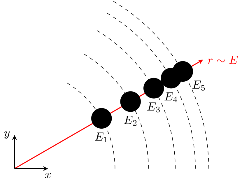
(a) Five bunches evolving radially on axis due to the isochronism of the cyclotron. The origin of the coordinate system denotes the center of the machine. The orbit radius $r$ of each bunch is proportional to its energy $E_{1}<E_{2}<\dots<E_{5}.$

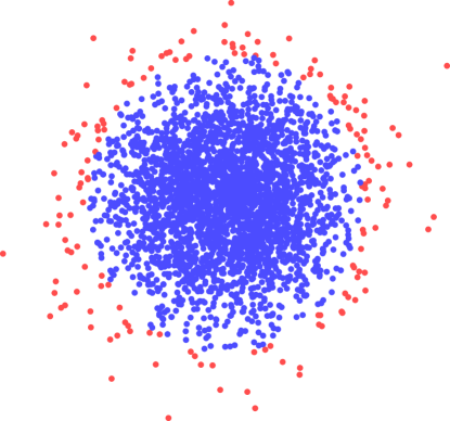
(b) Separation of a particle bunch into core (blue) and halo (red) particles. In the PSI Ring the overall loss is on the order of $10^{-4}$ which corresponds to a beam intensity of about $0.2\text{\,}\mathrm{\SIUnitSymbolMicro}\mathrm{A}$, i.e. all particles outside of approximately $3\sigma$ of a Gaussian distribution with standard deviation $\sigma$.

Figure 1: Sketch of neighbouring bunches (left) in the context of isochronous cyclotrons and characterization of a single bunch (right).

2.1.1 Numerical Model

The numerical model of neighbouring bunch simulations in OPAL, as presented in [11], is based on [10]. Due to the energy difference of the particle bunches on neighbouring turns a single transformation into the particle rest frame does not fully satisfy the requirements of the electrostatic assumption to solve Poisson’s equation. Instead, each of the $N$ macro particles is assigned to an energy bin $b$ due to its momentum $\beta\gamma$ according to

$$b=\Bigg{\lfloor}\frac{\operatorname{sinh^{-1}}{\left(\beta\gamma\right)}-\operatorname{sinh^{-1}}{\left(\min_{i=\{1,N\}}(\beta\gamma)_{i}\right)}}{\eta}\Bigg{\rfloor}$$ (1)

where the binning parameter $\eta$ is a measure of the energy spread. In each time step the force on a particle exerted by all others is the sum of the electric field contributions of each energy bin $b$ evaluated in the appropriate rest frame of the particles obtained by a Lorentz transform with the proper relativistic factor $\gamma_{b}$. The algorithm is summarised in Alg. 1. The computation of the electric field of an energy bin involves only particles of that bin, thus, the charge deposition applies only on a subset of particles $M\subset{\{1,\dots,N\}}$. However, the field on the mesh is interpolated and applied to all $N$ particles.

1:${\bf E}_{n}\leftarrow{\bf 0}\quad\forall n\in\{1,\dots,N\}$ // Electric field at particle location

2:for $b\in\{1,\dots,B\}$ do// Loop over energy bins

3:    ${\bf\tilde{x}}_{n}\leftarrow$LorentzTransform(${\bf x}_{n},\gamma_{b}$)$\quad\forall n\in\{1,\dots,N\}$

4:    $\tilde{\rho}_{i,j,k}\leftarrow$DepositCharge(${\bf\tilde{x}}_{m},q_{m}$) $\quad\forall m\in M\subset{\{1,\dots,N\}}$ // Interpolate charge onto mesh

5:    ${\bf\tilde{E}}_{i,j,k}^{b}\leftarrow$PoissonSolve($\tilde{\rho}_{i,j,k}$)

6:    ${\bf\tilde{E}}_{n}^{b}\leftarrow$ GatherEfield(${\bf\tilde{E}}_{i,j,k}^{b},{\bf\tilde{x}}_{n}$)$\quad\forall n\in\{1,\dots,N\}$ // Get field at particle location

7:    ${\bf E}_{n}^{b}\leftarrow$BackLorentzTransform(${\bf\tilde{E}}_{n}^{b},\gamma_{b}$) $\quad\forall n\in\{1,\dots,N\}$

8:    ${\bf x}_{n}\leftarrow$BackLorentzTransform(${\bf\tilde{x}}_{n},\gamma_{b}$)$\quad\forall n\in\{1,\dots,N\}$

9:    ${\bf E}_{n}\leftarrow{\bf E}_{n}+{\bf E}_{n}^{b}\quad\forall n\in\{1,\dots,N\}$ // Add field contribution

10:end for

Algorithm 1 Electrostatic Particle-In-Cell with $B$ energy bins and $N$ macro particles.

2.1.2 RF Electron Gun Model

To study the effect of energy binning we further use the example of the Argonne Wakefield Accelerator (AWA) [29, 30, 31] facility, an experiment setup for beam physics studies and accelerator technology developments. The facility is equipped with a photocathode rf electron gun that emits high intensity electron beams at high accelerating gradients ($\gg$1\text{\,}\mathrm{M}\mathrm{V}\mathrm{/}\mathrm{m}$$). Due to the high gradients the electrostatic approximation is invalidated and, hence, energy binning is necessary. In OPAL, we model the particle emission by

$$p_{total} =\sqrt{\left(\frac{E_{kin}}{mc^{2}}+1\right)^{2}-1}$$

$$p_{x} =p_{total}\sin\left(\varphi\right)\cos\left(\theta\right)$$

$$p_{y} =p_{total}\sin\left(\varphi\right)\sin\left(\theta\right)$$

$$p_{z} =p_{total}\left|\cos\left(\varphi\right)\right|$$

$$\varphi =2\cos^{-1}\left(\sqrt{x}\right)$$

with $x\in[0,1]$ and $\theta\in[0,\pi]$ uniformly randomly sampled [12].

2.2 Quantities of interest

In accelerator physics interesting quantities of interest (QoI) also denoted as observables, of the co-moving frame are the rms beam size

$$\sigma_{\omega}=\sqrt{\langle\omega^{2}\rangle}\quad\forall\omega=x,y,z$$

and the projected emittance

$$\varepsilon_{\omega}=\sqrt{\langle\omega^{2}\rangle\langle p_{\omega}^{2}\rangle-\langle\omega p_{\omega}\rangle^{2}}$$ (2)

that describes the phase space volume per dimension. The bracket $\langle\cdot\rangle$ represents the moment. In order to quantify halo (cf. Fig. 1(b)), i.e. the tails of a particle distribution, we use two statistical definitions for bunched beams by [32, 33], the spatial-profile parameter

$$h_{\omega}=\frac{\langle\omega^{4}\rangle}{\sigma_{\omega}^{4}}-\frac{15}{7}$$ (3)

and the phase-space halo parameter

$$H_{\omega}=\frac{\sqrt{3}}{2}\frac{\sqrt{I_{4}^{\omega}}}{\varepsilon_{\omega}^{2}}-\frac{15}{7}$$ (4)

with Eq. (2) and fourth order invariant (cf. also [34])

$$I_{4}^{\omega}=\left\langle\omega^{4}\right\rangle\left\langle p_{\omega}^{4}\right\rangle+3\left\langle\omega^{2}p_{\omega}^{2}\right\rangle^{2}-4\left\langle\omega p_{\omega}^{3}\right\rangle\left\langle\omega^{3}p_{\omega}\right\rangle.$$

In case the bunch has uniform density Eq. (3) is zero due to the constant $15/7$. An important quantity of interest in the rf electron gun model is the energy spread

$$\Delta E\propto\sqrt{\langle p_{z}^{2}\rangle}.$$ (5)

3 Non-Intrusive Uncertainty Quantification

Simulations of physical phenomena usually rely on measured input data. Depending on the accuracy of the measurement and the model sensitivity, the response may vary significantly. UQ introduces methods to quantify this variability in order to estimate the reliability of the obtained results. UQ distinguishes two approaches which are called intrusive and non-intrusive UQ. In contrast to intrusive UQ, non-intrusive UQ uses the computational model as a black box. In this paper we only give a short overview following the description and notation of [5, 9, 1, 35, 36]. A detailed introduction to UQ in general is found in e.g. [37, 38].

In Sec. 3.1, the surrogate model based on the polynomial chaos expansion (PCE) is explained in general. The sections 3.2 to 3.5 describe methods to obtain the coefficients of the expansion where special focus is given on the methods applied in this paper. The definition of the Sobol’ indices and their computation with the PCE is given in Sec. 3.6. In order to check the error bounds of the estimated sensitivities, we use the bootstrap method explained in Sec. 3.7.

3.1 Surrogate Model based on Polynomial Chaos Expansion

The PC-decomposition originates from [39], where a random variable of a Gaussian distribution is represented as a series of multivariate Hermite polynomials of increasing order. And as stated by the Cameron-Martin theorem [40], any functional in $L_{2}$ space can be represented in a series of Fourier-Hermite functionals. Later, this method was rediscovered and applied by [41] to a stochastic process and then generalized by [42] to other probability measures and their corresponding orthogonal polynomials.

Let a multivariate polynomial $\Psi_{\boldsymbol{\alpha}_{i}}(\boldsymbol{\xi})$ of dimension $d\in\mathbb{N}\setminus\{0\}$ and multiindex $\boldsymbol{\alpha}_{i}=(\alpha_{1},\alpha_{2},\dots,\alpha_{d})\in\mathbb{N}^{d}$ be defined by

$$\Psi_{\boldsymbol{\alpha}_{i}}(\boldsymbol{\xi})=\prod_{j=1}^{d}\psi_{\alpha_{j}}(\xi_{j})$$

with orthogonal univariate polynomials $\{\psi_{\alpha_{j}}\}_{j=1}^{d}$. The response of a model $m(\boldsymbol{x})$ with random input vector $\boldsymbol{x}\in\Omega_{1}\times\dots\times\Omega_{d}$, where $\Omega_{j}~{}\forall j=\{1,\dots,d\}$ denotes the sample space of the $j$-th random variable, can then be represented as

$$m(\boldsymbol{x})=\sum_{i=0}^{\infty}c_{\boldsymbol{\alpha}_{i}}\Psi_{\boldsymbol{\alpha}_{i}}(\mathcal{T}(\boldsymbol{x}))$$ (6)

where the basis of a random input component is determined by its probability distribution (cf. Tab. 1) and $\mathcal{T}:\boldsymbol{x}\mapsto\boldsymbol{\xi}$ denotes an isoprobabilistic transform. In case of dependent input components, for example, $\mathcal{T}$ represents the Rosenblatt transform [43] that yields independent random variables. Another method for dependent variables presented in [44] applies the Gram-Schmidt orthogonalization.

Under the assumption of only independent input variables, the transform $\mathcal{T}$ reduces to a simple linear mapping of every component of $\boldsymbol{x}$ onto the defined interval of the corresponding univariate polynomial, e.g. $\xi_{j}\in[-1,1]$ for Legendre polynomials. In numerical computations the sum in Eq. (6) is truncated at some polynomial degree $p$, hence the expansion is only an approximation of the exact model $m(\boldsymbol{x})$, i.e.

$$\hat{m}(\boldsymbol{x})=\sum_{i=0}^{P-1}c_{\boldsymbol{\alpha}_{i}}\Psi_{\boldsymbol{\alpha}_{i}}(\mathcal{T}(\boldsymbol{x})).$$ (7)

The truncation scheme is not clearly defined. A common rule, which is also used here, is the so-called total order truncation that keeps all multiindices $\boldsymbol{\alpha}$ for which $\left\lvert\left\lvert\boldsymbol{\alpha}\right\rvert\right\rvert_{1}\leq p$. This yields a number of

$$P=\frac{(p+d)!}{p!d!}$$ (8)

multiindices. Three other schemes are explained in [35]. In the next sections we describe methods to compute the coefficients $c_{\boldsymbol{\alpha}_{i}}$ of Eq. (7).

PDF of $\xi_{j}$	Polynomial Basis	Support
	$\{\psi_{\alpha_{j}}(\xi_{j})\}$	$\Omega_{j}$
Gaussian	Hermite	$]-\infty,\infty[$
Gamma	Laguerre	$[0,\infty[$
Uniform	Legendre	$[a,b]$ with $a,b\in\mathbb{R}$

Table 1: Examples of the Wiener-Askey polynomial chaos of random variables $\xi_{j}$ with appropriate probability density function (PDF) [42].

3.2 Projection Method

The (spectral) projection method computes the coefficients of Eq. (7) making use of the orthogonality of the basis functions, i.e. $\left\langle\Psi_{\boldsymbol{\alpha}_{i}}(\boldsymbol{\xi})\Psi_{\boldsymbol{\alpha}_{j}}(\boldsymbol{\xi})\right\rangle=0$ with $\forall i\neq j$. Thus, the PC coefficients are given by

$$c_{\boldsymbol{\alpha}_{i}}=\frac{\left\langle m(\mathcal{T}^{-1}(\boldsymbol{\xi}))\Psi_{\boldsymbol{\alpha}_{i}}(\boldsymbol{\xi})\right\rangle}{\left\langle\Psi_{\boldsymbol{\alpha}_{i}}^{2}(\boldsymbol{\xi})\right\rangle}.$$

While the denominator is evaluated by analytic formulas (see examples in the appendix of [9]), the numerator is computed by Gaussian quadrature integration where

$$N=(p+1)^{d}$$

integration points, i.e. high fidelity model $m(\boldsymbol{x})$ evaluations, are required.

3.3 Linear Regression Method

The coefficients of Eq. (7) can also be computed with regression-based methods

$$\boldsymbol{\hat{c}}=\operatorname*{arg\,min}_{\boldsymbol{c}}\frac{1}{2}\left\lvert\left\lvert\sum_{j=0}^{N-1}\left(m(\boldsymbol{x}_{j})-\sum_{i=0}^{P-1}c_{\boldsymbol{\alpha}_{i}}\Psi_{\boldsymbol{\alpha}_{i}}(\boldsymbol{\xi}_{j})\right)\right\rvert\right\rvert_{2}^{2}+\frac{\lambda_{1}}{2}\left\lvert\left\lvert\boldsymbol{c}\right\rvert\right\rvert_{2}^{2}+\lambda_{2}\left\lvert\left\lvert\boldsymbol{c}\right\rvert\right\rvert_{1}$$ (9)

with regularization parameters $\lambda_{1},\lambda_{2}\geq 0$, and the $l_{1}$ norm and $l_{2}$ norm denoted by $\left\lvert\left\lvert\cdot\right\rvert\right\rvert_{1}$ and $\left\lvert\left\lvert\cdot\right\rvert\right\rvert_{2}$, respectively. The minimization problem is called ordinary least squares if $\lambda_{1}=\lambda_{2}=0$, elastic net [45] if $\lambda_{1},\lambda_{2}>0$, ridge regression [46] (or Tikhonov regularization) if only $\lambda_{1}>0$ and Lasso [47] if only $\lambda_{2}>0$. In matrix form the problem reads

$$\boldsymbol{\hat{c}}=\operatorname*{arg\,min}_{\boldsymbol{c}}\frac{1}{2}\left\lvert\left\lvert\boldsymbol{y}-A\boldsymbol{c}\right\rvert\right\rvert_{2}^{2}+\frac{\lambda_{1}}{2}\left\lvert\left\lvert\boldsymbol{c}\right\rvert\right\rvert_{2}^{2}+\lambda_{2}\left\lvert\left\lvert\boldsymbol{c}\right\rvert\right\rvert_{1}$$ (10)

with model response $\boldsymbol{y}=\left(m(\boldsymbol{x}_{0}),\dots,m(\boldsymbol{x}_{N-1})\right)^{\intercal}\in\mathbb{R}^{N\times 1}$, unknown coefficient vector $\boldsymbol{c}=\left(c_{\boldsymbol{\alpha}_{0}},\dots,c_{\boldsymbol{\alpha}_{p}}\right)^{\intercal}\in\mathbb{R}^{P\times 1}$ and system matrix $A\in\mathbb{R}^{N\times P}$. In case of $\lambda_{2}=0$, the coefficients of Eq. (10) are obtained in closed form by

$$\boldsymbol{\hat{c}}=\left(A^{\intercal}A+\lambda_{1}I\right)^{-1}A^{\intercal}\boldsymbol{y}$$

with $P\times P$ identity matrix $I$. In contrast to the projection method (cf. Sec. 3.2), this method does not require a fixed number of samples $N$. However, [9] gives an empirical optimal training sample size of

$$N=(d-1)P$$ (11)

with $P$ defined in Eq. (8).

3.4 Orthogonal Matching Pursuit

The matching pursuit (MP) is a greedy algorithm developed by [18] which was enhanced by [19] to obtain better convergence. This improved method is called orthogonal MP (OMP). In terms of PCE, the algorithm searches a minimal set of non-zero coefficients to represent the model response, i.e.

$$\boldsymbol{\hat{c}}=\operatorname*{arg\,min}_{\boldsymbol{c}} \left\lvert\left\lvert\boldsymbol{y}-A\boldsymbol{c}\right\rvert\right\rvert_{2}^{2}$$

subject to $$\left\lvert\left\lvert\boldsymbol{c}\right\rvert\right\rvert_{0}\leq N_{c}$$

where $\left\lvert\left\lvert\boldsymbol{c}\right\rvert\right\rvert_{0}$ denotes the number of non-zero coefficients in $\boldsymbol{c}$ with a user-defined maximum $N_{c}$ [48]. The vectors and matrices are defined according to Eq. (10). It is an iterative procedure where in the $(i+1)$-th step a new coefficient vector $\boldsymbol{c}_{i+1}$ is searched that maximizes the inner product to the current residual $\boldsymbol{r}_{i}=\boldsymbol{y}-\boldsymbol{y}_{i}$. We refer to the given references for details.

3.5 Bayesian Compressive Sensing

As stated in [14, 15], the linear regression model Eq. (9) can be interpreted in a Bayesian manner, i.e.

$$p\left(\boldsymbol{c}|\mathcal{D}\right)=\frac{p\left(\mathcal{D}|\boldsymbol{c}\right)p\left(\boldsymbol{c}\right)}{p\left(\mathcal{D}\right)}$$

with posterior distribution $p\left(\boldsymbol{c}|\mathcal{D}\right)$, likelihood $p\left(\mathcal{D}|\boldsymbol{c}\right)$, prior $p\left(\boldsymbol{c}\right)$ and evidence $p\left(\mathcal{D}\right)$ of training data $\mathcal{D}=\{\boldsymbol{x},y\}_{j=0}^{N-1}$ [36]. The likelihood is assigned a Gaussian noise model

$$p\left(\mathcal{D}|\boldsymbol{c}\right)=\frac{1}{\left(2\pi\sigma^{2}\right)^{N/2}}\exp\left(-\sum_{j=0}^{N-1}\frac{\left(m\left(\boldsymbol{x}_{i}\right)-\hat{m}\left(\boldsymbol{x}_{i}\right)\right)^{2}}{2\sigma^{2}}\right)$$

with variance $\sigma^{2}$. It is a measure of how well the high fidelity model is represented by the surrogate model Eq. (7). In order to favour a sparse PCE solution, a Laplace prior

$$p\left(\boldsymbol{c}\right)=\left(\frac{\lambda}{2}\right)^{P+1}\exp\left(-\lambda\sum_{i=0}^{P}\left|c_{i}\right|\right)$$ (12)

is chosen. Using Eq. (12) in the maximum a posteriori (MAP) estimate for $\boldsymbol{c}$, i.e.

$$\operatorname*{arg\,max}_{\boldsymbol{c}}{}\log\left[p\left(\mathcal{D}|\boldsymbol{c}\right)p\left(\boldsymbol{c}\right)\right],$$ (13)

the Bayesian approach is equivalent to Eq. (9) with $\lambda_{1}=0$ [49], since Eq. (13) is identical to a minimization of

$$\operatorname*{arg\,min}_{\boldsymbol{c}}{}-\log\left[p\left(\mathcal{D}|\boldsymbol{c}\right)p\left(\boldsymbol{c}\right)\right].$$

An iterative algorithm to obtain the coefficients is described in [15]. It requires a user-defined stopping threshold $\varepsilon$ that basically controls the number of kept basis terms, with more being skipped the higher the value is. The overall method is known as Bayesian Compressive Sensing (BCS) [14, 15].

3.6 Sensitivity Analysis

Sobol’ indices [1] are good measures of sensitivity since they provide information about single and mixed parameter effects. In addition to these sensitivity measures, there are various other methodologies such as Morris screening [50]. A survey is presented in [51] on the example of a hydrological model. Instead of Monte Carlo, Sobol’ indices are also easily obtained by surrogate models based on PCE as discussed in the following subsections.

3.6.1 Sobol’ Sensitivity Indices

In [1] Sobol’ proposed global sensitivity indices that are calculated on an analysis of variance (ANOVA) decomposition (Sobol’ decomposition) of a square integrable function $f(\boldsymbol{x})$ with $\boldsymbol{x}\in I^{d}\coloneqq[0,1]^{d}$, i.e. [52]

$$f(\boldsymbol{x})=f_{0}+\sum_{i=1}^{d}f_{i}(x_{i})+\sum_{1\leq i_{1}<\dots<i_{s}\leq d}f_{i_{1}i_{s}}(x_{i_{1}},x_{i_{s}})+\dots+f_{12\dots d}(x_{1},x_{2},\dots,x_{d})$$ (14)

with mean

$$f_{0}=\int_{I^{d}}f(\boldsymbol{x})\mathrm{d}\boldsymbol{x}$$

and

$$\int_{0}^{1}f_{i_{1}\dots i_{s}}(x_{i_{1}},\dots,x_{i_{s}})\mathrm{d}x_{k}=0,$$ (15)

for $k=i_{1},\dots,i_{s}$ and $s=1,\dots,d$. Since Eq. (15) holds, the components of Eq. (14) are mutually orthogonal. Therefore, the total variance of Eq. (14) is

$$D=\int_{I^{d}}f^{2}(\boldsymbol{x})\mathrm{d}\boldsymbol{x}-f_{0}^{2}$$

that can also be written as

$$D=\sum_{i=1}^{d}D_{i}+\sum_{1\leq i_{1}<\dots<i_{s}\leq d}D_{i_{1}i_{s}}+\dots+D_{123\dots d}$$ (16)

where

$$D_{i_{1}\dots i_{s}}=\int_{I^{s}}f_{i_{1}\dots i_{s}}^{2}(x_{i_{1}},\dots,x_{i_{s}})\mathrm{d}x_{i_{1}}\cdots\mathrm{d}x_{i_{s}},$$ (17)

with $1\leq i_{1}<\dots<i_{s}\leq d$. Based on Eq. (16) and Eq. (17), the Sobol’ indices are defined as

$$S_{i_{1}\dots i_{s}}\coloneqq\frac{D_{i_{1}\dots i_{s}}}{D}$$

with

$$\sum_{i=1}^{d}S_{i}+\sum_{1\leq i<j\leq d}S_{ij}+\dots+S_{12\dots d}=1.$$ (18)

The first order indices $S_{i}$ are also known as main sensitivities. They describe the effect of a single input parameter on the model response. The total effect of the $i$-th design variable on the model response, proposed by [53], is the sum of all Sobol’ indices that include the $i$-th index, i.e.

$$S_{i}^{T}=\sum_{\boldsymbol{i}\in\mathcal{I}}S_{\boldsymbol{i}}$$

with $\mathcal{I}=\{\boldsymbol{i}=(i_{1},\dots,i_{s}):\exists k,1\leq k\leq s\leq d,i_{k}=i\}$.

3.6.2 Sobol’ Indices using Polynomial Chaos Expansion

Instead of Monte Carlo techniques, Sobol’ indices can be estimated using surrogate models based on PCE since the truncated expansion can be rearranged like Eq. (14). The Sobol’ estimates are then given by [9]

$$\hat{S}_{i_{1}\dots i_{s}}=\frac{1}{\hat{D}}\sum_{\boldsymbol{\alpha}\in\mathcal{I}_{i_{1},\dots,i_{s}}}c_{\boldsymbol{\alpha}}^{2}\left\langle\Psi_{\boldsymbol{\alpha}}^{2}\right\rangle$$

where

$$\mathcal{I}_{i_{1},\dots,i_{s}}=\left\{\boldsymbol{\alpha}:\begin{matrix}\alpha_{k}>0&\forall k=1,\dots,n,\quad k\in\left(i_{1},\dots,i_{s}\right)\\ \alpha_{k}=0&\forall k=1,\dots,n,\quad k\not\in\left(i_{1},\dots,i_{s}\right)\end{matrix}\right\}$$

and variance

$$\hat{D}=\sum_{i=1}^{P-1}c_{\boldsymbol{\alpha}_{i}}^{2}\left\langle\Psi_{\boldsymbol{\alpha}_{i}}^{2}\right\rangle.$$

The main and total sensitivities are computed by

$$\hat{S}_{i}=\frac{1}{\hat{D}}\sum_{\boldsymbol{\alpha}\in\mathcal{I}_{i}}c_{\boldsymbol{\alpha}}^{2}\left\langle\Psi_{\boldsymbol{\alpha}}^{2}\right\rangle$$

with $\mathcal{I}_{i}=\{\boldsymbol{\alpha}=\left(\alpha_{1},\dots,\alpha_{d}\right):\alpha_{i}>0\wedge\forall k\neq i,\alpha_{k}=0\}$ and

$$\hat{S}_{i}^{T}=\frac{1}{\hat{D}}\sum_{\boldsymbol{\alpha}\in\mathcal{I}_{i}}c_{\boldsymbol{\alpha}}^{2}\left\langle\Psi_{\boldsymbol{\alpha}}^{2}\right\rangle,$$

with $\mathcal{I}_{i}=\{\boldsymbol{\alpha}=(\alpha_{1},\dots,\alpha_{d}):\alpha_{i}>0\}$, respectively.

3.7 Confidence Intervals using Bootstrap

In this subsection we briefly outline the computation of confidence intervals for the estimates of Sobol’ indices using the bootstrap method [54]. In the context of PCE, the bootstrap method has already been applied in [55], where it is referred to as bootstrap-PCE (or bPCE). The bootstrap method, in general, generates $B$ independent samples each of size $N$ by resampling from the original dataset. Each bootstrap sample, that may contain a point several times, is then considered as a new training sample to compute the coefficients of Eq. (7). In order to calculate the $95\text{\,}\mathrm{\char 37\relax}$ confidence interval for Sobol’ indices we follow the description of [56], where the bounds are given by

$$\hat{S}_{i_{1}\dots i_{s}}\pm 1.96\cdot s.e.(\hat{S}_{i_{1}\dots i_{s}})$$

with $1\leq s\leq d$ and standard error ($s.e.$) of $B\in\mathbb{N}^{>1}$ bootstrap samples

$$s.e.(\hat{S}_{i_{1}\dots i_{s}})=\sqrt{\frac{1}{B-1}\sum_{b=1}^{B}\left(S_{i_{1}\dots i_{s}}^{(b)}-S_{i_{1}\dots i_{s}}^{*}\right)^{2}}$$

and bootstrap sample mean

$$S_{i_{1}\dots i_{s}}^{*}=\frac{1}{B}\sum_{b=1}^{B}S_{i_{1}\dots i_{s}}^{(b)}.$$

4 Experiment Design

4.1 High Intensity Cyclotrons

In order to study the effect of AMR solver parameters and energy binning in neighbouring bunch simulations we perform sensitivity experiments with three different high intensity cyclotrons, the PSI Ring [57], the PSI Injector II [58] and the DAE$\delta$ALUS Injector Cyclotron (DIC) [27, 28]. We always accelerate 5 particle bunches with $10^{6}$ particles. The coarsest level grid is kept constant with $24^{3}$ mesh points which is refined twice. For the PSI Injector II and PSI Ring the particles are integrated in time over one turn using $2880$ steps per turn and for the DIC over three turns with $1440$ steps per turn. The experimental setup is summarized in Tab. 2. In all experiments the initial particle distribution is read from a checkpoint file to guarantee identical conditions for all training and validation points of a UQ sample.

no. turns	steps/turn	no. bunches	particles/bunch	PIC base grid	no. AMR levels
1 or 3	1440 or 2880	5	$10^{6}$	$24\times 24\times 24$	2

Table 2: Experimental setup of the PSI Ring, PSI Injector II and DAE$\delta$ALUS Injector Cyclotron model.

A list of the design variables under consideration is given in Tab. 3. While the resolution is basically controlled by the maximum number of AMR levels, the refinement policy affects its location. As described in [13] the OPAL library provides several refinement criteria such as the charge density per grid point, the potential as well as the electric field. Here, we want to analyze the effect of the threshold $\lambda\in[0,1]$ of the electrostatic potential refinement policy, where a grid cell $(i,j,k)$ on a level $l$ is refined if

$$|\phi^{l}_{i,j,k}|\geq\lambda\max_{i,j,k}|\phi^{l}_{i,j,k}|$$

holds. Due to the motion of the particles in space the multi-level hierarchy has to be updated regularly to maintain the resolution which is defined by the regrid frequency $f_{r}$. It should be noted that the regrid frequency defines the number of steps until the AMR hierarchy is updated. Hence, if $f_{r}=1$, the AMR levels are updated in each time step. Whenever this happens, the electric self-field needs to be recalculated by solving Poisson’s equation. The number of Poisson solves is controlled by the number of energy bins and therefore by the binning parameter $\eta$ (cf. Sec. 2.1.1). The lower the value of $\eta$, the smaller the bin width and, hence, the more expensive the model is.

As an upper limit of the regrid frequency $f_{r}$ we choose $120$ integration steps. Since we perform either $1440$ or $2880$ steps per turn, this corresponds to an azimuthal angle of $30\text{\,}\mathrm{\SIUnitSymbolDegree}$ and $15\text{\,}\mathrm{\SIUnitSymbolDegree}$, respectively. The choice of the binning parameter $\eta$ in Eq. (1) depends mainly on the energy difference between bunches. The upper bound of the sampling range was selected such that we have at most as many energy bins as bunches in simulation. However, the sampling from the range is not straightforward since there exist more states with fewer energy bins (cf. Fig. 2) due to Eq. (1). Instead, we sample the binning parameter in subranges of equal bin count in order to avoid a biased sample set.

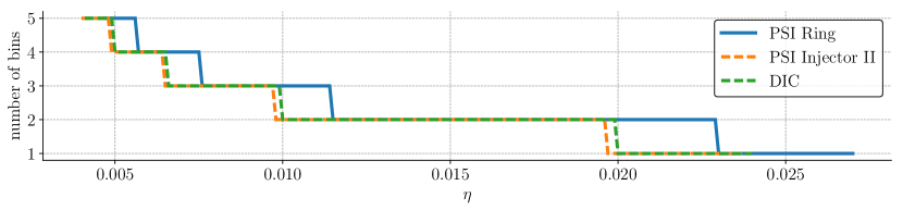
Figure 2: Number of energy bins in the PSI Ring, PSI Injector II and DAE$\delta$ALUS Injector Cyclotron (DIC) with respect to the binning parameter $\eta$. The shown binning curves are with respect to the initial simulation energies used in this study. A straightforward uniform sampling from the full range yields a biased sample set.

symbol	design variable	sampling range
$f_{r}$	regrid frequency	$[1,120]$
$\lambda$	refinement threshold	$[0.5,0.9]$
$\eta$	binning Ring $(10^{-3})$	$[4.7,5.7]\cup[5.8,7.6]\cup[7.7,11.5]\cup[11.6,23.0]\cup[23.1,27.1]$
	binning Inj-2 $(10^{-3})$	$[4.0,4.9]\cup[5.0,6.5]\cup[6.6,9.8]\cup[9.9,19.7]\cup[19.8,23.8]$
	binning DIC $(10^{-3})$	$[4.1,5.0]\cup[5.1,6.6]\cup[6.7,10.0]\cup[10.1,20.0]\cup[20.1,24.1]$

Table 3: List of design variables and their sampling ranges for the neighbouring bunch simulations.

4.2 RF Electron Gun Model

Like in the neighbouring bunch model, the time-to-solution in the rf electron gun model is dominated by the Poisson solver and the time integration. A reduction of the computational effort with regard to the Poisson solver is achieved by smaller PIC meshes and fewer energy bins $N_{E}$. The costs of the time integrator is cheapened with coarser time steps $\Delta t$ and fewer macro particles. Instead of the AMR model, the rf electron gun model uses the Fast Fourier Transform (FFT) Poisson solver of OPAL where we put a $L_{x}\times L_{y}\times L_{z}$ uniform mesh of $L_{x}=L_{y}=64$ and $L_{z}=32$ grid points. The final number of emitted macro particles is given by

$$N_{p}=p_{f}L_{x}L_{y}L_{z}$$

where the particle multiplication factor $p_{f}$ is an integer. This parameter basically controls the number of particles per grid cell and, hence, the noise of the PIC model. The design variables and sampling ranges are given in Tab. 4. We model the rf electron gun of the Argonne Wakefield Accelerator (AWA) that has a length of approximately $30\text{\,}\mathrm{c}\mathrm{m}$.

symbol	design variable	sampling range
$p_{f}$	particle factor	$[1,5]$
$N_{E}$	number of bins	$[2,10]$
$\Delta t$	time step $($0.1\text{\,}\mathrm{p}\mathrm{s}$)$	$[1,10]$

Table 4: List of design variables and their sampling ranges for the rf electron gun model. The time step is the only floating point variable.

4.3 Surrogate Model Selection

In order to avoid overfitting we proceed like [35] where the truncation order of the PC expansion and the settings of the regression models are chosen such that the relative $l_{2}$ error

$$\sqrt{\frac{\sum_{i=0}^{N-1}\left[m(\boldsymbol{x}_{i})-\hat{m}(\boldsymbol{x}_{i})\right]^{2}}{\sum_{i=0}^{N-1}m^{2}(\boldsymbol{x}_{i})}}$$ (19)

between the surrogate $\hat{m}(\boldsymbol{x})$ and high fidelity model $m(\boldsymbol{x})$ of the training and validation set is approximately of equal magnitude. As an additional error measure we also compare the relative $l_{1}$ error

$$\frac{\sum_{i=0}^{N-1}\left|m(\boldsymbol{x}_{i})-\hat{m}(\boldsymbol{x}_{i})\right|}{\sum_{i=0}^{N-1}\left|m(\boldsymbol{x}_{i})\right|}.$$ (20)

The number of samples $N$ in Eq. (19) and Eq. (20) corresponds either to the number of training $N_{t}$ or validation points $N_{v}$. The total number of $N=100$ samples was randomly partitioned into disjoint training and validation sets with $N_{t}=0.5N$ and $N_{v}=0.5N$, respectively. Since we have $d=3$ design variables, we satisfy Eq. (11) with $N_{t}=50$ up to polynomial order $p=3$.

5 Results

The estimated sensitivities are obtained from PC surrogate models where we use either ordinary least squares (OLS) and Bayesian compressive sensing (BCS) of UQTk [16, 17] or orthogonal matching pursuit (OMP) of scikit-learn [20, 21] together with Chaospy [7] to compute the expansion coefficients. A summary of the PC model setups is given in Tab. 5. In order to study the evolution of the sensitivities we construct the PC surrogate models at equidistant steps of the accelerator models and evaluate their sensitivities. These steps correspond to azimuthal angles in the cyclotrons or longitudinal positions in the rf electron gun model. In the examples below we only show the first order Sobol’ indices since their sum is already almost one which is the maximum per definition (cf. Eq. (18)).

model	PC order	stopping criterion
		$\varepsilon$ (BCS)	$N_{c}$ (OMP)
PSI Ring	2	$1.0\text{\times}{10}^{-7}$	5
PSI Injector II	2	$1.0\text{\times}{10}^{-4}$	7
DIC	2	$1.0\text{\times}{10}^{-8}$	6
AWA	2	$1.0\text{\times}{10}^{-9}$	7

Table 5: PC surrogate model settings for all accelerator model examples. The stopping criterion of Bayesian Compressive Sensing (BCS) and Orthogonal Matching Pursuit (OMP) is discussed in Sec. 3.5 and Sec. 3.4, respectively.

5.1 High Intensity Cyclotrons

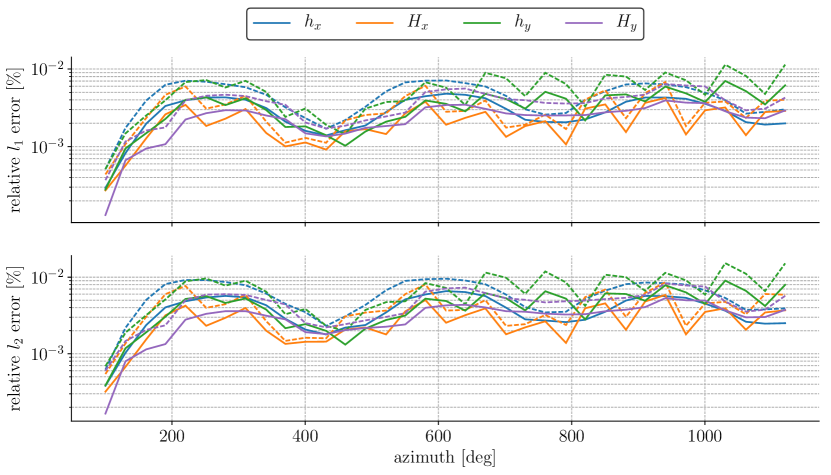
Figure 8: Evolution of the relative $l_{2}$ and $l_{1}$ error between the surrogate and the true model of the DAE$\delta$ALUS Injector Cyclotron. The full lines are the errors to the surrogate model obtained with the training set and the dashed lines are the errors to the surrogate model computed with the validation set. For each quantity, the dashed and full lines are close to each other, indicating no overfitting of the surrogate model.

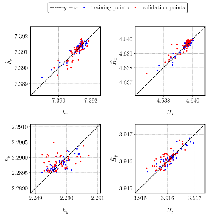
Figure 9: Comparison between the high fidelity ($x$-axis) and PC surrogate model ($y$-axis) at $1120.395\text{\,}\mathrm{\SIUnitSymbolDegree}$ of the DAE$\delta$ALUS Injector Cyclotron simulation. The blue and red dots indicate the training and validation points, respectively. In the best case all points coincide with the dashed black line.

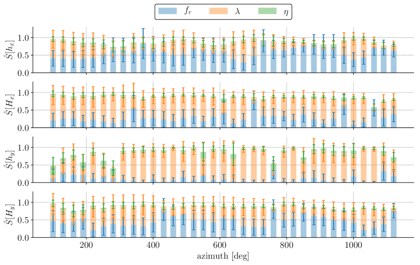
Figure 10: Evolution of the estimated first order Sobol’ indices in the DAE$\delta$ALUS Injector Cyclotron. The error bars denote the $95\text{\,}\mathrm{\char 37\relax}$ bootstrapped $(B=100)$ confidence interval (cf. Sec. 3.7). The main sensitivities are evaluated for the spatial-profile parameters $h_{x}$, $h_{y}$ and the phase-space halo parameters $H_{x}$, $H_{y}$ as defined in Eq. (3) and Eq. (4), respectively. The bars are coloured with respect to the regrid frequency $f_{r}$, AMR refinement threshold $\lambda$ and energy binning parameter $\eta$. Beside the refinement threshold, the regrid frequency has also a significant impact on the halo measures.

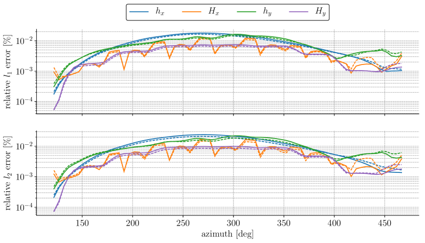
Figure 12: Evolution of the relative $l_{2}$ and $l_{1}$ error between the surrogate and the true model of the PSI Ring cyclotron. The full lines are the errors to the surrogate model obtained with the training set and the dashed lines are the errors to the surrogate model computed with the validation set. For each quantity, the dashed and full lines are close to each other, indicating no overfitting of the surrogate model.

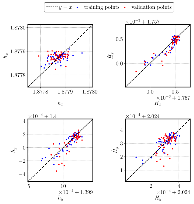
Figure 13: Comparison between the high fidelity ($x$-axis) and PC surrogate model ($y$-axis) at $470.79\text{\,}\mathrm{\SIUnitSymbolDegree}$ of the PSI Ring simulation. The blue and red dots indicate the training and validation points, respectively. In the best case all points coincide with the dashed black line.

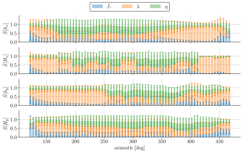
Figure 14: Evolution of the estimated first order Sobol’ indices in the PSI Ring. The error bars denote the $95\text{\,}\mathrm{\char 37\relax}$ bootstrapped $(B=100)$ confidence interval (cf. Sec. 3.7). The main sensitivities are evaluated for the spatial-profile parameters $h_{x}$, $h_{y}$ and the phase-space halo parameters $H_{x}$, $H_{y}$ as defined in Eq. (3) and Eq. (4), respectively. The bars are coloured with respect to the regrid frequency $f_{r}$, AMR refinement threshold $\lambda$ and energy binning parameter $\eta$. Due to the high uncertainty of the sensitivities, no reliable conclusion can be drawn for this machine.

In order to study the effect of the input parameters we evaluate the sensitivities of the halo parameters Eq. (3) and Eq. (4) with respect to the center bunch of the 5 bunches (cf. Fig. 1(a)). The initial kinetic energy of the center bunch in the different models is approximately $98\text{\,}\mathrm{M}\mathrm{e}\mathrm{V}$, $25\text{\,}\mathrm{M}\mathrm{e}\mathrm{V}$ and $17\text{\,}\mathrm{M}\mathrm{e}\mathrm{V}$ for the PSI Ring, PSI Injector II and DIC, respectively. As shown in Fig. 4, Fig. 8 and Fig. 12, the relative $l_{1}$ and $l_{2}$ errors (cf. Eq. (20) and Eq. (19)) between training and test samples are in good agreement for all cyclotron examples. A similar observation is done at a single angle in Fig. 5, Fig. 9 and Fig. 13. The average errors are given in Tab. 7, Tab. 8 and Tab. 9. The computation methods OLS, BCS and OMP yield similar results. In case of the PSI Injector II, the refinement threshold has more than $80\text{\,}\mathrm{\char 37\relax}$ impact on the halo. The energy binning parameter $\eta$ and regrid frequency $f_{r}$ play a negligible role. The increase of the $95\text{\,}\mathrm{\char 37\relax}$ bootstrap confidence intervals in Fig. 6 correlates with the decrease of the standard deviation in Fig. 3. It is best observed for $h_{x}$ at around $215\text{\,}\mathrm{\SIUnitSymbolDegree}$ or $H_{x}$ between $195\text{\,}\mathrm{\SIUnitSymbolDegree}$ and $255\text{\,}\mathrm{\SIUnitSymbolDegree}$. In contrast to the PSI Injector II, the DIC also strongly depends on the regrid frequency. It has an average main sensitivity of approximately $60\text{\,}\mathrm{\char 37\relax}$ for $h_{x}$. The parameters also exhibit more correlations as observed between the main and total sensitivities (cf. Tab. 8). The standard deviations for the DIC are one order of magnitude smaller than for the PSI Injector II, causing the confidence intervals to increase as illustrated in Fig. 10. This effect is even stronger in the PSI Ring where Coulomb’s repulsion is less dominant and the halo parameters are smaller (cf. Fig. 11) compared to the PSI Injector II. The standard deviation is in the order of $\mathcal{O}(10^{-4})$ denoting no significant influence of the input parameters on the model response, hence, the confidence intervals in Fig. 14 exhibit large ranges. For this reason we can make no reliable statement about the sensitivities for the PSI Ring. Nevertheless, these findings give rise to computational savings. Due to the small deviations, it is sufficient for the PSI Ring to select a cheap model. According to Tab. 6, the cheapest model among all $N=100$ samples is $2.470\,773\,495$ times faster than the most expensive model.

model	design variables			time [$\mathrm{s}$]
	$f_{r}$	$\lambda$	$\eta$
PSI Ring	$111$	$0.827\,205\,906\,368\,997$	$0.022\,692\,320\,324\,177\,9$	$7937.66$
	$3$	$0.502\,208\,846\,849\,441$	$0.005\,212\,093\,058\,299\,28$	$19\,612.6$
PSI Injector II	$4$	$0.645\,451\,840\,951\,718$	$0.022\,381\,889\,183\,628\,7$	$10\,526.2$
	$3$	$0.502\,208\,846\,849\,441$	$0.004\,460\,883\,752\,469\,35$	$21\,422.1$
DIC	$90$	$0.858\,436\,519\,969\,397\,29$	$0.015\,726\,255\,173\,021\,168$	$9559.72$
	$74$	$0.595\,824\,756\,266\,788\,99$	$0.021\,640\,390\,914\,407\,701$	$31\,709.4$

Table 6: Most expensive and cheapest cyclotron models with respect to runtime among all $N=100$ samples.

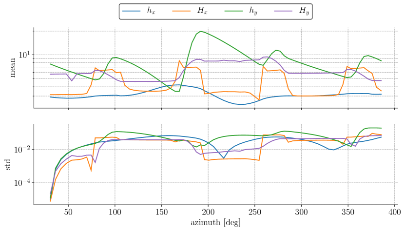
Figure 3: Evolution of the mean and standard deviation (std) of the spatial-profile parameters $h_{x}$, $h_{y}$ and the phase-space halo parameters $H_{x}$, $H_{y}$ as defined in Eq. (3) and Eq. (4), respectively. Based on the mean of $H_{x}$, the location of the dipoles in the PSI Injector II can be detected, i.e. at $90\text{\,}\mathrm{\SIUnitSymbolDegree}$, $180\text{\,}\mathrm{\SIUnitSymbolDegree}$, $270\text{\,}\mathrm{\SIUnitSymbolDegree}$ and $360\text{\,}\mathrm{\SIUnitSymbolDegree}$.

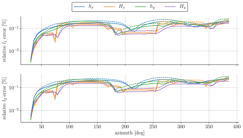
Figure 4: Evolution of the relative $l_{2}$ and $l_{1}$ error between the surrogate and the true model of the PSI Injector II. The full lines are the errors to the surrogate model obtained with the training set and the dashed lines are the errors to the surrogate model computed with the validation set. For each quantity, the dashed and full lines are close to each other, indicating no overfitting of the surrogate model.

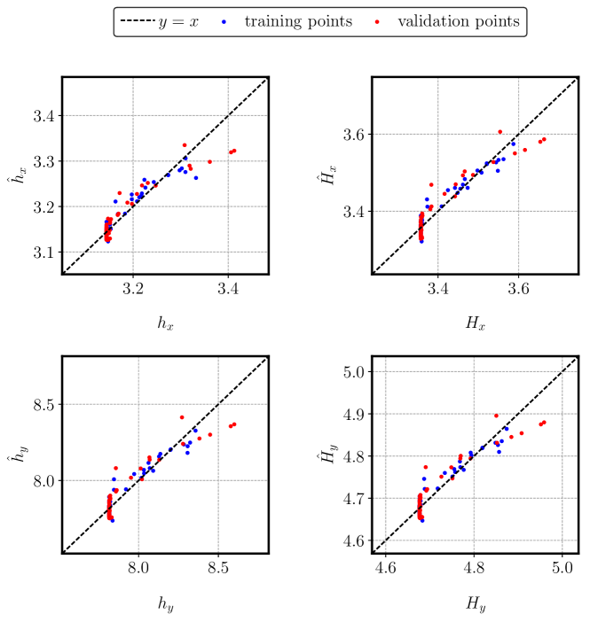
Figure 5: Comparison between the high fidelity ($x$-axis) and PC surrogate model ($y$-axis) at $389.76\text{\,}\mathrm{\SIUnitSymbolDegree}$ of the PSI Injector II simulation. The blue and red dots indicate the training and validation points, respectively. In the best case all points coincide with the dashed black line.

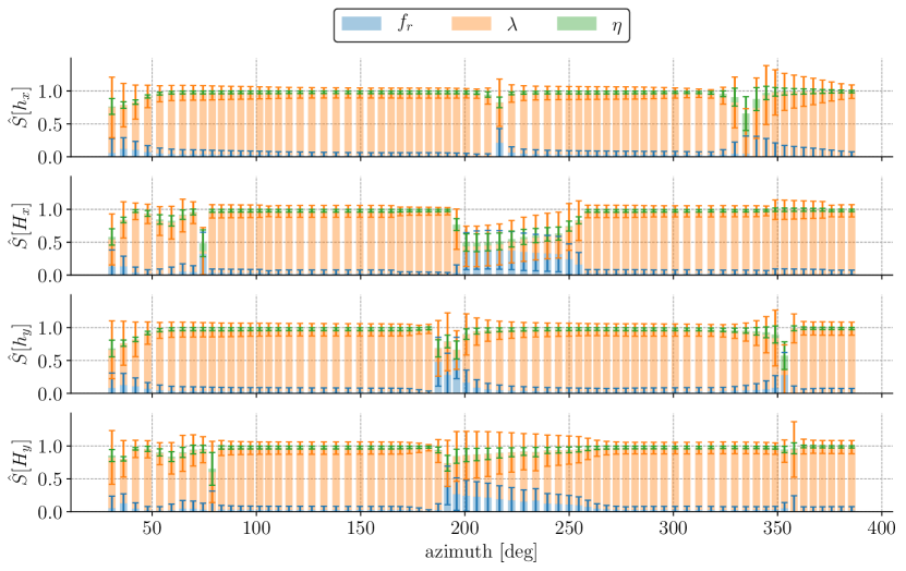
Figure 6: Evolution of the estimated first order Sobol’ indices in the PSI Injector II. The error bars denote the $95\text{\,}\mathrm{\char 37\relax}$ bootstrapped $(B=100)$ confidence interval (cf. Sec. 3.7). The main sensitivities are evaluated for the spatial-profile parameters $h_{x}$, $h_{y}$ and the phase-space halo parameters $H_{x}$, $H_{y}$ as defined in Eq. (3) and Eq. (4), respectively. The bars are coloured with respect to the regrid frequency $f_{r}$, AMR refinement threshold $\lambda$ and energy binning parameter $\eta$. The refinement threshold has the highest impact on the halo measures.

QoI	method	$l_{1}$ error [$\mathrm{\char 37\relax}$]		$l_{2}$ error [$\mathrm{\char 37\relax}$]		Sobol’ sensitivity indices
		train	test	train	test	$\hat{S}_{f_{r}}$	$\hat{S}_{f_{r}}^{T}$	$\hat{S}_{\lambda}$	$\hat{S}_{\lambda}^{T}$	$\hat{S}_{\eta}$	$\hat{S}_{\eta}^{T}$
$h_{x}$	OLS	$0.232\,821\,859\,621$	$0.330\,311\,686\,12$	$0.325\,169\,056\,284$	$0.443\,290\,907\,933$	$0.033\,283\,216\,431\,7$	$0.056\,919\,978\,830\,4$	$0.911\,940\,255\,097$	$0.942\,184\,764\,242$	$0.015\,530\,643\,421\,5$	$0.040\,144\,058\,141\,1$
	BCS	$0.257\,338\,954\,498$	$0.296\,255\,360\,765$	$0.378\,130\,065\,003$	$0.442\,985\,128\,941$	$0.029\,982\,514\,054\,4$	$0.051\,732\,989\,838\,2$	$0.918\,573\,246\,082$	$0.946\,823\,461\,362$	$0.015\,143\,968\,892$	$0.037\,745\,315\,176$
	OMP	$0.243\,060\,322\,065$	$0.317\,087\,569\,515$	$0.342\,042\,936\,791$	$0.451\,375\,236\,579$	$0.025\,824\,193\,153\,1$	$0.044\,920\,698\,246\,5$	$0.922\,471\,367\,016$	$0.948\,979\,550\,726$	$0.016\,901\,859\,241\,2$	$0.040\,902\,331\,617\,5$
$H_{x}$	OLS	$0.148\,205\,498\,661$	$0.221\,405\,898\,725$	$0.205\,247\,578\,735$	$0.291\,173\,389\,144$	$0.078\,967\,183\,829\,5$	$0.161\,929\,025\,011$	$0.804\,487\,851\,808$	$0.889\,096\,567\,287$	$0.014\,892\,050\,188\,3$	$0.050\,634\,563\,096\,5$
	BCS	$0.164\,648\,808\,34$	$0.196\,712\,500\,816$	$0.242\,120\,670\,319$	$0.283\,876\,688\,118$	$0.074\,097\,134\,302$	$0.154\,141\,237\,27$	$0.814\,520\,580\,464$	$0.896\,304\,217\,515$	$0.014\,347\,244\,061$	$0.046\,597\,912\,201$
	OMP	$0.154\,400\,093\,72$	$0.213\,103\,179\,933$	$0.215\,910\,814\,09$	$0.295\,954\,037\,154$	$0.070\,586\,062\,162\,4$	$0.162\,239\,790\,01$	$0.803\,543\,357\,493$	$0.898\,243\,201\,997$	$0.014\,709\,649\,056\,9$	$0.050\,677\,939\,281\,3$
$h_{y}$	OLS	$0.184\,056\,392\,662$	$0.273\,807\,830\,239$	$0.254\,739\,486\,285$	$0.363\,653\,831\,697$	$0.058\,024\,450\,188\,9$	$0.099\,978\,128\,335$	$0.876\,138\,850\,97$	$0.915\,229\,996\,67$	$0.011\,747\,957\,993\,6$	$0.038\,893\,677\,174\,6$
	BCS	$0.200\,391\,486\,694$	$0.239\,731\,290\,676$	$0.299\,284\,454\,823$	$0.353\,022\,457\,333$	$0.050\,894\,649\,165\,2$	$0.094\,169\,887\,657$	$0.882\,519\,868\,621$	$0.923\,567\,655\,954$	$0.011\,757\,881\,058$	$0.037\,098\,536\,844\,5$
	OMP	$0.190\,515\,298\,291$	$0.261\,395\,763\,441$	$0.268\,628\,573\,041$	$0.368\,172\,349\,073$	$0.049\,185\,260\,33$	$0.084\,450\,981\,666\,6$	$0.888\,950\,703\,942$	$0.923\,090\,157\,184$	$0.013\,516\,942\,109\,9$	$0.040\,805\,954\,768\,3$
$H_{y}$	OLS	$0.107\,423\,276\,534$	$0.165\,587\,296\,093$	$0.147\,401\,293\,434$	$0.219\,008\,577\,268$	$0.059\,516\,299\,690\,4$	$0.100\,453\,925\,054$	$0.878\,863\,744\,688$	$0.918\,049\,699\,489$	$0.008\,709\,995\,355\,68$	$0.034\,407\,669\,222\,2$
	BCS	$0.118\,521\,563\,913$	$0.145\,609\,358\,176$	$0.174\,598\,998\,574$	$0.212\,125\,190\,429$	$0.057\,605\,670\,450\,6$	$0.096\,771\,984\,020\,2$	$0.883\,131\,079\,495$	$0.921\,055\,066\,205$	$0.008\,302\,699\,368\,31$	$0.033\,134\,443\,411\,3$
	OMP	$0.111\,484\,167\,055$	$0.159\,928\,095\,49$	$0.155\,275\,012\,987$	$0.222\,871\,258\,764$	$0.050\,324\,061\,348\,2$	$0.086\,349\,523\,483\,9$	$0.889\,733\,763\,289$	$0.927\,077\,170\,279$	$0.008\,801\,723\,212\,26$	$0.037\,713\,758\,388\,1$

Table 7: Average relative $l_{1}$ and $l_{2}$ errors between the high fidelity model and the PC surrogate models for the training and validation sets as well as the average main and total sensitivities for the PSI Injector II. OLS: Ordinary Least Squares; BCS: Bayesian Compressive Sensing; OMP: Orthogonal Matching Pursuit.

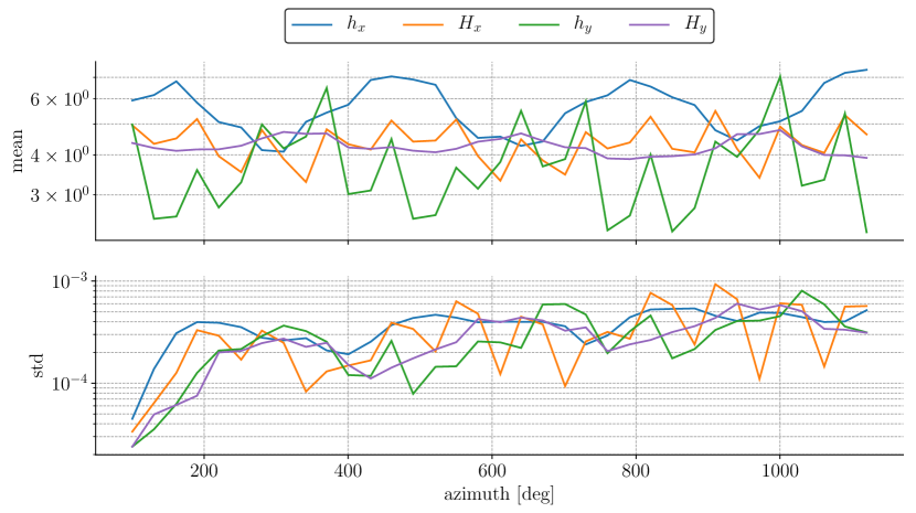
Figure 7: Evolution of the mean and standard deviation (std) of the spatial-profile parameters $h_{x}$, $h_{y}$ and the phase-space halo parameters $H_{x}$, $H_{y}$ as defined in Eq. (3) and Eq. (4), respectively. The mean of all quantities shows a more or less periodic pattern along the three turns of the DAE$\delta$ALUS Injector Cyclotron.

QoI	method	$l_{1}$ error [$10^{-2}$$\mathrm{\char 37\relax}$]		$l_{2}$ error [$10^{-2}$$\mathrm{\char 37\relax}$]		Sobol’ sensitivity indices
		train	test	train	test	$\hat{S}_{f_{r}}$	$\hat{S}_{f_{r}}^{T}$	$\hat{S}_{\lambda}$	$\hat{S}_{\lambda}^{T}$	$\hat{S}_{\eta}$	$\hat{S}_{\eta}^{T}$
$h_{x}$	OLS	$0.002\,944\,524\,593\,08$	$0.004\,544\,534\,466\,17$	$0.003\,824\,976\,568\,74$	$0.006\,053\,105\,608\,9$	$0.591\,202\,348\,746$	$0.706\,129\,435\,228$	$0.265\,261\,396\,713$	$0.334\,730\,768\,575$	$0.016\,449\,878\,403\,6$	$0.086\,227\,640\,77$
	BCS	$0.003\,000\,543\,983\,19$	$0.004\,580\,947\,693\,4$	$0.003\,922\,826\,382\,03$	$0.006\,083\,716\,376\,21$	$0.599\,446\,635\,564$	$0.715\,895\,492\,045$	$0.254\,150\,529\,693$	$0.325\,473\,002\,264$	$0.016\,450\,330\,626\,6$	$0.088\,585\,456\,275\,3$
	OMP	$0.002\,998\,582\,708\,09$	$0.004\,471\,772\,985\,27$	$0.003\,946\,077\,406\,18$	$0.005\,997\,680\,710\,7$	$0.616\,075\,462\,855$	$0.717\,722\,883\,017$	$0.264\,766\,841\,987$	$0.319\,504\,157\,065$	$0.011\,504\,571\,790\,5$	$0.070\,426\,083\,285\,8$
$H_{x}$	OLS	$0.002\,149\,093\,278\,72$	$0.003\,135\,483\,929\,91$	$0.002\,783\,042\,035\,36$	$0.004\,121\,998\,450\,88$	$0.288\,755\,932\,821$	$0.398\,769\,861\,025$	$0.565\,778\,200\,161$	$0.669\,472\,377\,271$	$0.021\,156\,561\,482\,9$	$0.056\,069\,186\,005$
	BCS	$0.002\,252\,817\,044\,97$	$0.003\,173\,121\,726\,03$	$0.002\,959\,087\,650\,17$	$0.004\,154\,894\,857\,27$	$0.287\,237\,458\,849$	$0.396\,879\,006\,02$	$0.568\,823\,684\,46$	$0.672\,081\,853\,888$	$0.020\,157\,295\,996\,4$	$0.054\,822\,597\,970\,3$
	OMP	$0.002\,345\,277\,193\,79$	$0.003\,091\,356\,191\,31$	$0.003\,058\,261\,069\,61$	$0.004\,024\,461\,698\,04$	$0.252\,230\,120\,309$	$0.343\,830\,126\,599$	$0.644\,293\,223\,368$	$0.725\,082\,153\,242$	$0.009\,649\,906\,277\,73$	$0.024\,914\,470\,204\,4$
$h_{y}$	OLS	$0.003\,409\,124\,537\,98$	$0.005\,541\,809\,516\,53$	$0.004\,402\,250\,598\,19$	$0.007\,177\,906\,575\,59$	$0.106\,374\,659\,724$	$0.239\,196\,354\,928$	$0.674\,270\,839\,39$	$0.764\,424\,681\,492$	$0.069\,542\,584\,610\,8$	$0.146\,196\,868\,37$
	BCS	$0.003\,465\,292\,871\,54$	$0.005\,459\,912\,148\,69$	$0.004\,456\,860\,702\,75$	$0.007\,057\,567\,126\,03$	$0.106\,200\,719\,907$	$0.239\,379\,101\,085$	$0.673\,901\,118\,492$	$0.764\,202\,010\,497$	$0.069\,676\,211\,092\,1$	$0.146\,649\,757\,605$
	OMP	$0.003\,585\,432\,664\,39$	$0.005\,371\,453\,602\,17$	$0.004\,578\,467\,875\,61$	$0.006\,888\,068\,654\,04$	$0.101\,900\,162\,904$	$0.221\,518\,800\,453$	$0.712\,196\,987\,592$	$0.773\,835\,606\,696$	$0.061\,005\,594\,389$	$0.129\,542\,847\,966$
$H_{y}$	OLS	$0.002\,421\,850\,860\,71$	$0.003\,676\,595\,214\,69$	$0.003\,116\,601\,016\,9$	$0.004\,708\,985\,874\,97$	$0.467\,787\,967\,483$	$0.578\,066\,105\,013$	$0.388\,597\,334\,787$	$0.477\,511\,892\,662$	$0.018\,859\,505\,802\,6$	$0.069\,185\,813\,254\,1$
	BCS	$0.002\,450\,619\,598\,43$	$0.003\,805\,672\,488\,49$	$0.003\,176\,355\,347\,99$	$0.004\,878\,540\,312\,43$	$0.467\,000\,202\,266$	$0.577\,418\,574\,766$	$0.389\,491\,110\,328$	$0.478\,403\,710\,86$	$0.018\,774\,859\,129\,9$	$0.068\,919\,496\,690\,2$
	OMP	$0.002\,538\,815\,019\,86$	$0.003\,678\,256\,047\,98$	$0.003\,299\,218\,924\,84$	$0.004\,665\,102\,885\,48$	$0.436\,631\,187\,74$	$0.534\,512\,594\,83$	$0.455\,310\,318\,398$	$0.525\,769\,056\,283$	$0.008\,639\,633\,315\,31$	$0.039\,137\,209\,432\,9$

Table 8: Average relative $l_{1}$ and $l_{2}$ errors between the high fidelity model and the PC surrogate models for the training and validation sets as well as the average main and total sensitivities for the DAE$\delta$ALUS Injector Cyclotron. OLS: Ordinary Least Squares; BCS: Bayesian Compressive Sensing; OMP: Orthogonal Matching Pursuit.

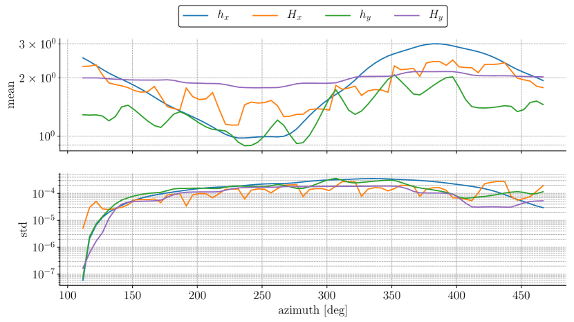
Figure 11: Evolution of the mean and standard deviation (std) of the spatial-profile parameters $h_{x}$, $h_{y}$ and the phase-space halo parameters $H_{x}$, $H_{y}$ as defined in Eq. (3) and Eq. (4), respectively. The variability of these quantities in the PSI Ring cyclotron is on the order of $\mathcal{O}(10^{-4})$ which is two orders of magnitude smaller than for the PSI Injector II (cf. Fig. 3).

QoI	method	$l_{1}$ error [$10^{-2}$$\mathrm{\char 37\relax}$]		$l_{2}$ error [$10^{-2}$$\mathrm{\char 37\relax}$]		Sobol’ sensitivity indices
		train	test	train	test	$\hat{S}_{f_{r}}$	$\hat{S}_{f_{r}}^{T}$	$\hat{S}_{\lambda}$	$\hat{S}_{\lambda}^{T}$	$\hat{S}_{\eta}$	$\hat{S}_{\eta}^{T}$
$h_{x}$	OLS	$0.008\,462\,169\,169\,24$	$0.007\,806\,918\,328\,99$	$0.011\,271\,879\,296\,4$	$0.010\,121\,325\,664\,3$	$0.149\,564\,698\,832$	$0.193\,514\,991\,919$	$0.502\,307\,714\,343$	$0.544\,650\,075\,988$	$0.272\,360\,345\,065$	$0.337\,610\,396\,784$
	BCS	$0.009\,190\,785\,954\,62$	$0.008\,015\,773\,678\,49$	$0.012\,414\,467\,553\,4$	$0.010\,552\,557\,051\,2$	$0.150\,116\,844\,068$	$0.194\,318\,598\,477$	$0.500\,931\,023\,206$	$0.542\,756\,695\,765$	$0.273\,150\,475\,296$	$0.338\,735\,998\,094$
	OMP	$0.008\,649\,894\,638\,22$	$0.007\,838\,570\,513\,38$	$0.011\,426\,833\,122\,7$	$0.010\,079\,951\,023\,7$	$0.136\,369\,694\,631$	$0.161\,875\,388\,105$	$0.500\,412\,321\,81$	$0.508\,579\,420\,757$	$0.336\,377\,012\,981$	$0.356\,386\,161\,717$
$H_{x}$	OLS	$0.004\,721\,630\,718\,74$	$0.004\,463\,175\,886\,95$	$0.006\,234\,524\,873\,37$	$0.005\,789\,818\,217\,2$	$0.106\,656\,445\,07$	$0.162\,918\,577\,49$	$0.592\,377\,759\,679$	$0.620\,656\,635\,265$	$0.223\,437\,409\,262$	$0.293\,955\,700\,649$
	BCS	$0.005\,982\,217\,666\,46$	$0.005\,013\,673\,908\,8$	$0.007\,859\,110\,163\,08$	$0.006\,452\,954\,222\,26$	$0.105\,142\,411\,058$	$0.162\,074\,439\,71$	$0.593\,584\,665\,138$	$0.621\,889\,908\,22$	$0.222\,980\,027\,494$	$0.294\,331\,253\,212$
	OMP	$0.004\,841\,637\,722\,08$	$0.004\,485\,701\,385\,94$	$0.006\,359\,776\,900\,94$	$0.005\,692\,627\,859\,51$	$0.066\,596\,657\,848\,1$	$0.127\,171\,361\,122$	$0.634\,645\,132\,509$	$0.636\,749\,596\,708$	$0.238\,183\,506\,369$	$0.296\,653\,745\,444$
$h_{y}$	OLS	$0.008\,009\,240\,928\,79$	$0.007\,568\,165\,123\,83$	$0.010\,507\,953\,178\,3$	$0.009\,801\,429\,944\,02$	$0.102\,610\,063\,899$	$0.185\,343\,809\,241$	$0.597\,300\,143\,85$	$0.631\,890\,288\,136$	$0.204\,240\,535\,349$	$0.278\,616\,854\,186$
	BCS	$0.009\,560\,548\,980\,38$	$0.008\,048\,449\,258\,12$	$0.012\,792\,448\,361\,9$	$0.010\,639\,683\,677\,7$	$0.102\,418\,438\,962$	$0.185\,249\,557\,747$	$0.597\,505\,793\,032$	$0.632\,039\,321\,571$	$0.204\,164\,696\,684$	$0.278\,623\,934\,309$
	OMP	$0.008\,140\,573\,497\,2$	$0.007\,689\,914\,306\,57$	$0.010\,666\,349\,692\,5$	$0.009\,820\,447\,161\,54$	$0.088\,486\,958\,172\,9$	$0.165\,845\,172\,023$	$0.588\,217\,322\,146$	$0.606\,066\,207\,961$	$0.236\,689\,129\,702$	$0.314\,695\,209\,995$
$H_{y}$	OLS	$0.004\,173\,769\,301\,54$	$0.003\,853\,124\,941\,14$	$0.005\,517\,695\,917\,52$	$0.004\,972\,268\,623\,9$	$0.129\,490\,345\,249$	$0.219\,391\,367\,739$	$0.510\,831\,201\,465$	$0.554\,174\,815\,745$	$0.250\,473\,440\,194$	$0.335\,749\,781\,728$
	BCS	$0.004\,741\,335\,725\,41$	$0.003\,879\,234\,854\,79$	$0.006\,230\,228\,345\,55$	$0.004\,939\,953\,340\,84$	$0.134\,308\,726\,874$	$0.226\,938\,365\,147$	$0.501\,128\,720\,261$	$0.546\,888\,520\,138$	$0.250\,512\,277\,877$	$0.340\,311\,450\,774$
	OMP	$0.004\,280\,880\,036\,66$	$0.004\,040\,447\,403\,93$	$0.005\,637\,241\,264\,05$	$0.004\,991\,641\,062\,5$	$0.097\,665\,161\,021\,5$	$0.226\,235\,305\,757$	$0.523\,683\,635\,99$	$0.540\,477\,683\,772$	$0.244\,576\,318\,139$	$0.367\,361\,895\,321$

Table 9: Average relative $l_{1}$ and $l_{2}$ errors between the high fidelity model and the PC surrogate models for the training and validation sets as well as the average main and total sensitivities for the PSI Ring. OLS: Ordinary Least Squares; BCS: Bayesian Compressive Sensing; OMP: Orthogonal Matching Pursuit.

5.2 RF Electron Gun Model

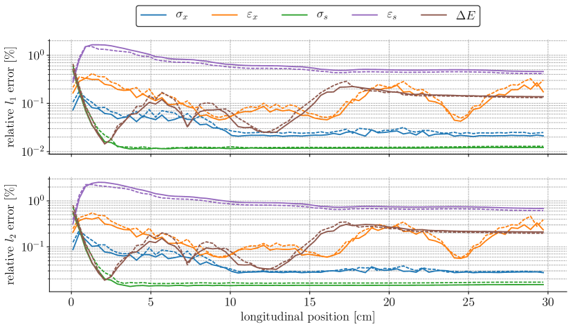
Figure 16: Evolution of the relative $l_{2}$ and $l_{1}$ error between the surrogate and the true model of the AWA rf electron gun. The full lines are the errors to the surrogate model obtained with the training set and the dashed lines are the errors to the surrogate model computed with the validation set. For each quantity, the dashed and full lines are close to each other, indicating no overfitting of the surrogate model.

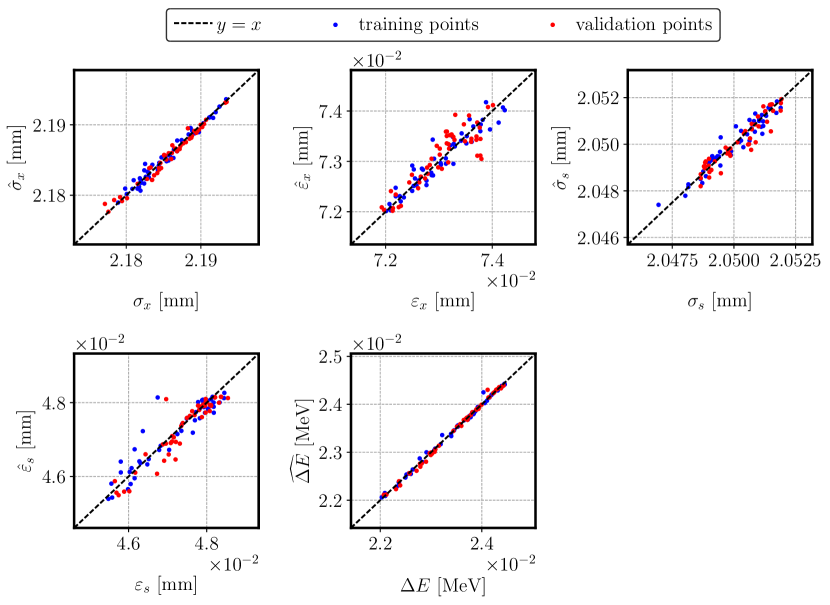
Figure 17: Comparison between the high fidelity ($x$-axis) and PC surrogate model ($y$-axis) at the exit of the rf electron gun model of the AWA, i.e. $s\approx$30\text{\,}\mathrm{c}\mathrm{m}$$. The blue and red dots indicate the training and validation points, respectively. In the best case all points coincide with the dashed black line.

In order to approximate the high fidelity model we use PC surrogate models of second order where the BCS method uses a tolerance of $\varepsilon=10^{-9}$ and the OMP method is stopped once 7 non-zero coefficients are found. In Fig. 16 are the relative $l_{2}$ and $l_{1}$ errors evaluated along the rf electron gun model. The mean errors are summarized in Tab. 10. It shows that the $l_{1}$ and $l_{2}$ errors on the test and training points match with an absolute difference of $\mathcal{O}(10^{-2})$ and $\mathcal{O}(10^{-1})$, respectively. An example of a comparison between the PC surrogate and high fidelity model is illustrated in Fig. 17.

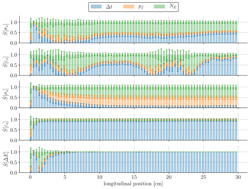
Figure 18: Evolution of the estimated first order Sobol’ indices in the rf electron gun model of the AWA. The error bars denote the $95\text{\,}\mathrm{\char 37\relax}$ bootstrapped $(B=100)$ confidence interval (cf. Sec. 3.7). The main sensitivities are evaluated for the energy spread $\Delta E$, the projected emittances $\varepsilon_{x}$, $\varepsilon_{s}$ and the rms beam sizes $\sigma_{x}$, $\sigma_{s}$. The bars are coloured with respect to the time step $\Delta t$, particle multiplication factor $p_{f}$ and the number of energy bins $N_{E}$. The impact of the parameters on the quantities in longitudinal direction converges.

The first order Sobol’ indices and their $95\text{\,}\mathrm{\char 37\relax}$ bootstrapped confidence intervals are illustrated in Fig. 18. Except to the sensitivities of the horizontal projected emittance $\varepsilon_{x}$, we observe a convergence of the model parameter influences. The energy spread $\Delta E$ and the projected emittance $\varepsilon_{s}$ strongly depend on the time step ($\hat{S}[\varepsilon_{s}],\hat{S}[\Delta E]>0.90$). This high influence is due to the momentum component in their definitions (cf. Eq. (5) and Eq. (2)) and the fact that the smaller the time step, the better the process of acceleration (i.e. the evolution of the momentum) is resolved. The rms beam size in longitudinal direction is dominated by the energy binning ($\hat{S}[N_{E}]\approx 0.45$) and the particle multiplication factor ($\hat{S}[p_{f}]\approx 0.41$). While a higher $p_{f}$ value improves the statistics of the beam size and reduces the numerical noise of PIC, the energy binning is coupled with Coulomb’s repulsion that affects the beam size. In transverse direction, $N_{E}$ and $\Delta t$ are important instead. The convergence of the relative errors is correlated with the convergence of the variances of the quantities of interest as observed in Fig. 15. The model might therefore be improved with an adaptive time stepping scheme that addresses this effect. The cheapest AWA rf electron gun model, i.e. $\Delta t=$1\text{\,}\mathrm{p}\mathrm{s}$$, $N_{E}=2$ and $p_{f}=1$, is $15.237\,717\,908$ times faster than the most expensive model which has $\Delta t=$0.1\text{\,}\mathrm{p}\mathrm{s}$$, $N_{E}=10$ and $p_{f}=5$.

QoI	method	$l_{1}$ error [$\mathrm{\char 37\relax}$]		$l_{2}$ error [$\mathrm{\char 37\relax}$]		Sobol’ sensitivity indices
		train	test	train	test	$\hat{S}_{\Delta t}$	$\hat{S}_{\Delta t}^{T}$	$\hat{S}_{p_{f}}$	$\hat{S}_{p_{f}}^{T}$	$\hat{S}_{N_{E}}$	$\hat{S}_{N_{E}}^{T}$
$\sigma_{x}$	OLS	$0.033\,756\,115\,251\,3$	$0.040\,115\,848\,304\,8$	$0.043\,284\,644\,277\,2$	$0.049\,525\,790\,428\,4$	$0.317\,231\,191\,336$	$0.321\,293\,769\,766$	$0.118\,960\,256\,283$	$0.121\,559\,097\,556$	$0.558\,751\,198\,852$	$0.562\,204\,486\,889$
	BCS	$0.037\,510\,031\,408\,1$	$0.042\,494\,825\,422\,9$	$0.047\,694\,935\,522\,3$	$0.052\,633\,898\,612\,5$	$0.317\,231\,245\,341$	$0.321\,293\,723\,198$	$0.118\,960\,205\,139$	$0.121\,558\,962\,72$	$0.558\,751\,322\,113$	$0.562\,204\,542\,181$
	OMP	$0.034\,234\,586\,839\,4$	$0.039\,953\,376\,369\,6$	$0.043\,974\,700\,397\,4$	$0.048\,944\,100\,945\,2$	$0.320\,301\,605\,606$	$0.323\,015\,745\,883$	$0.121\,658\,066\,876$	$0.122\,919\,744\,397$	$0.554\,655\,554\,331$	$0.557\,449\,282\,905$
$\varepsilon_{x}$	OLS	$0.128\,644\,137\,131$	$0.156\,742\,084\,063$	$0.163\,378\,794\,155$	$0.198\,031\,850\,182$	$0.433\,188\,470\,507$	$0.443\,277\,695\,714$	$0.092\,698\,318\,483\,5$	$0.099\,417\,337\,834\,4$	$0.461\,647\,098\,119$	$0.469\,771\,079\,479$
	BCS	$0.136\,254\,491\,327$	$0.154\,709\,687\,587$	$0.173\,074\,898\,196$	$0.194\,918\,196\,446$	$0.433\,223\,011\,013$	$0.443\,176\,165\,331$	$0.092\,733\,634\,789\,4$	$0.099\,341\,647\,131\,8$	$0.461\,720\,910\,044$	$0.469\,804\,631\,831$
	OMP	$0.131\,395\,584\,226$	$0.156\,920\,045\,831$	$0.165\,841\,989\,519$	$0.197\,615\,124\,755$	$0.439\,830\,037\,115$	$0.448\,175\,514\,92$	$0.095\,892\,210\,423$	$0.101\,166\,452\,233$	$0.453\,845\,672\,93$	$0.461\,090\,112\,379$
$\sigma_{s}$	OLS	$0.021\,452\,253\,273\,9$	$0.024\,590\,744\,235\,3$	$0.026\,242\,557\,633\,2$	$0.031\,754\,088\,835$	$0.131\,912\,434\,386$	$0.137\,392\,208\,661$	$0.408\,145\,899\,229$	$0.410\,322\,235\,549$	$0.454\,068\,394\,908$	$0.458\,158\,832\,62$
	BCS	$0.021\,971\,410\,574\,3$	$0.026\,853\,871\,754$	$0.028\,278\,535\,284\,3$	$0.034\,236\,188\,948\,3$	$0.131\,912\,613\,948$	$0.137\,392\,326\,1$	$0.408\,145\,520\,001$	$0.410\,321\,790\,665$	$0.454\,068\,679\,868$	$0.458\,159\,075\,069$
	OMP	$0.021\,771\,286\,689\,5$	$0.024\,971\,923\,628\,7$	$0.026\,787\,766\,637\,1$	$0.031\,708\,146\,807\,5$	$0.132\,622\,266\,46$	$0.134\,354\,362\,331$	$0.387\,640\,274\,979$	$0.388\,378\,729\,587$	$0.477\,944\,909\,877$	$0.479\,059\,456\,768$
$\varepsilon_{s}$	OLS	$0.694\,447\,125\,841$	$0.616\,410\,825\,971$	$1.041\,291\,980\,63$	$0.929\,607\,880\,117$	$0.946\,356\,614\,3$	$0.956\,278\,013\,311$	$0.007\,758\,009\,996\,87$	$0.008\,519\,181\,758\,43$	$0.035\,873\,190\,709\,6$	$0.045\,214\,989\,928\,2$
	BCS	$0.925\,594\,370\,168$	$0.860\,688\,730\,597$	$1.219\,188\,104\,86$	$1.123\,725\,708\,59$	$0.946\,581\,221\,681$	$0.956\,227\,460\,319$	$0.007\,853\,087\,644\,83$	$0.008\,637\,771\,054\,23$	$0.035\,828\,554\,531\,3$	$0.044\,871\,904\,773\,1$
	OMP	$0.694\,242\,824\,635$	$0.625\,872\,178\,206$	$1.044\,666\,057\,1$	$0.947\,515\,919\,23$	$0.946\,914\,401\,994$	$0.957\,263\,379\,485$	$0.007\,616\,925\,920\,26$	$0.008\,090\,843\,616\,39$	$0.035\,119\,694\,595$	$0.044\,994\,754\,39$
$\Delta E$	OLS	$0.114\,272\,864\,138$	$0.123\,998\,435\,711$	$0.159\,888\,329\,298$	$0.167\,836\,845\,715$	$0.942\,337\,717\,858$	$0.944\,768\,577\,303$	$0.008\,715\,120\,909\,48$	$0.010\,352\,951\,464\,8$	$0.046\,187\,900\,566\,8$	$0.047\,637\,732\,148\,4$
	BCS	$0.143\,833\,321\,344$	$0.154\,745\,425\,134$	$0.184\,751\,110\,548$	$0.194\,996\,806\,352$	$0.942\,386\,571\,447$	$0.944\,799\,182\,955$	$0.008\,689\,200\,459\,55$	$0.010\,331\,091\,657\,6$	$0.046\,183\,643\,104\,5$	$0.047\,610\,310\,601\,5$
	OMP	$0.114\,617\,904\,809$	$0.122\,852\,848\,97$	$0.161\,503\,666\,19$	$0.165\,561\,315\,705$	$0.942\,284\,146\,628$	$0.944\,272\,594\,05$	$0.008\,446\,253\,891\,3$	$0.009\,567\,204\,793\,45$	$0.047\,091\,544\,113\,7$	$0.048\,338\,256\,524$

Table 10: Average relative $l_{1}$ and $l_{2}$ errors between the high fidelity model and the PC surrogate models for the training and validation sets as well as the average main and total sensitivities for the rf electron gun model of the AWA. OLS: Ordinary Least Squares; BCS: Bayesian Compressive Sensing; OMP: Orthogonal Matching Pursuit.

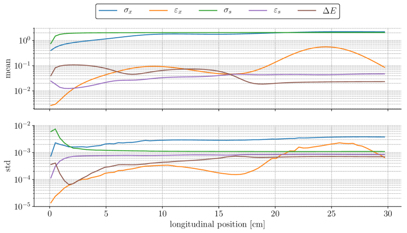
Figure 15: Evolution of the mean and standard deviation (std) of the energy spread $\Delta E$, the projected emittances $\varepsilon_{x}$, $\varepsilon_{s}$ and the rms beam sizes $\sigma_{x}$, $\sigma_{s}$ for rf electron gun model of the AWA.

6 Conclusions

In this paper we discussed uncertainty quantification based on polynomial chaos expansion and gave a brief introduction to four numerical methods to compute the polynomial coefficients. The choice of the method depends on the problem and its dimension. While the projection method is the most accurate, the number of high-fidelity evaluations grows exponentially with the dimension which is not the case for the other presented methods. Bayesian compressive sensing and matching orthogonal pursuit favour sparse solutions by the selection of the most important contributions. The least squares method solves a linear system which may fail in case the matrix is ill-conditioned which happens when input dimensions can only take a few discrete values. This can be the case with integer input, for example, when specifying the number of AMR levels or the grid sizes for the Poisson solver.

Beside a cheap surrogate model that mimics the high fidelity model, polynomial chaos based uncertainty quantification has the additional benefit to easily evaluate the Sobol’ sensitivity indices. As demonstrated in this paper, this technique is not only suitable to gain knowledge about the sensitivity of physical parameters (e.g. initial beam properties) on the quantities of interest but also numerical parameters of computer codes. Since some tested numerical parameters might be limited to integers, the projection method to obtain the polynomial coefficients is, however, not applicable. Instead, regression-based methods, Bayesian Compressive Sensing or Orthogonal Matching Pursuit and others have to be applied. A further difficulty with numerical parameters is a fair random sampling. In some cases (cf. Fig. 2) a straightforward, uniform sampling of the parameter yields biased input data and, hence, may induce wrong conclusions. To circumvent, we perform a stratified sampling that guarantees a well-balanced distribution.

The sensitivity studies of the three high intensity cyclotrons show that the sensitivity results are different among accelerators of the same type. While the AMR threshold is the most important parameter in the PSI Injector II with a sensitivity of about $90\text{\,}\mathrm{\char 37\relax}$, the regrid frequency is relevant in the DAE$\delta$ALUS Injectory Cyclotron (DIC), too. Large bootstrap confidence intervals for the Sobol’ indices indicate a failure of the analysis since the contributed variation of the model response is rather due to noise than the tested input parameters. In such a case no reliable statements based on the sensitivity estimates can be done. In contrast to our intuition the standard deviation of the halo parameters remain pretty constant throughout one turn in the PSI Ring and PSI Injector II and the considered three turns in the DIC. Nevertheless, these findings give rise to computational savings. Without losing significantly on accuracy (cf. Fig. 3, Fig. 7 and Fig. 11), energy binning can be totally switched off for these cyclotrons. In addition, this reduces the amount of AMR hierarchy updates which reduces the time-to-solution even further since the operators of the adaptive multigrid solver to solve Poisson’s equation do not need to be set up in every time step. To illustrate this, we take the benchmark example in [13] that solves Poisson’s equation 100 times using a three level AMR hierarchy with a base level of $576^{3}$ grid points. The benchmark running on $14\,400$ CPU (Central Processing Unit) cores shows that the matrix setup due to AMR regriding takes up $42.15\text{\,}\mathrm{\char 37\relax}$ computing time. A reduction of the regrid frequency by a factor 10 yields a speedup of $7.097\,821\,254$ in the matrix setup timing. In our UQ samples, the speedup between the cheapest and most expensive model is at least $2.0$ and at most $3.3$.

Another interesting case we have studied is the rf electron gun model of the AWA. Relevant parameters for this model are the energy binning $N_{E}$ and the time step $\Delta t$. The particle multiplication factor $p_{f}$, that basically controls the number of particles per grid cell, is only important for the longitudinal beam size. Although $N_{E}$ and $p_{f}$ have together an average main sensitivity of $86.22\text{\,}\mathrm{\char 37\relax}$, $\Delta t$ is the dominating parameter close to the cathode. An adaptive energy binning and time step scheme that is based on Sobol’ sensitivity indices is therefore a possible future enhancement to reduce the time-to-solution for a target accuracy.

7 Acknowledgments

The authors thank the developers of UQTk, especially B. Debusschere and K. Sargsyan. The computer resources were provided by the Swiss National Supercomputing Centre (CSCS), Paul Scherrer Institut (PSI) and the Laboratory Computing Resource Center at the Argonne National Laboratory (ANL). This project is funded by the Swiss National Science Foundation (SNSF) under contract number 200021_159936.

References

- [1] Sobol’, I. M., Mathematics and Computers in Simulation 55 (2001) 271, The Second IMACS Seminar on Monte Carlo Methods.
- [2] Najm, H. N., Annual Review of Fluid Mechanics 41 (2009) 35.
- [3] Reagan, M. T. et al., Combustion Theory and Modelling 8 (2004) 607.
- [4] Eck, V. G. et al., International Journal for Numerical Methods in Biomedical Engineering 32 (2016) e02755.
- [5] Adelmann, A., SIAM/ASA Journal on Uncertainty Quantification 7 (2019) 383.
- [6] Marelli, S. and Sudret, B., UQLab: A Framework for Uncertainty Quantification in Matlab, in Vulnerability, Uncertainty, and Risk, Second International Conference on Vulnerability and Risk Analysis and Management (ICVRAM) and the Sixth International Symposium on Uncertainty, Modeling, and Analysis (ISUMA), pages 2554–2563, 2014.
- [7] Feinberg, J. and Langtangen, H. P., Journal of Computational Science 11 (2015) 46 .
- [8] Adams, B. M. et al., Dakota, a multilevel parallel object-oriented framework for design optimization, parameter estimation, uncertainty quantification, and sensitivity analysis: Version 6.0 user’s manual, 2014, Sandia Technical Report SAND2014-4633, Updated November 2015 (Version 6.3).
- [9] Sudret, B., Reliability Engineering & System Safety 93 (2008) 964 , Bayesian Networks in Dependability.
- [10] Fubiani, G., Qiang, J., Esarey, E., Leemans, W. P., and Dugan, G., Phys. Rev. ST Accel. Beams 9 (2006) 064402.
- [11] Yang, J. J., Adelmann, A., Humbel, M., Seidel, M., and Zhang, T. J., Phys. Rev. ST Accel. Beams 13 (2010) 064201.
- [12] Adelmann, A. et al., arXiv e-prints (2019) arXiv:1905.06654.
- [13] Frey, M., Adelmann, A., and Locans, U., Computer Physics Communications (2019) 106912.
- [14] Ji, S., Xue, Y., and Carin, L., IEEE Transactions on Signal Processing 56 (2008) 2346.
- [15] Babacan, S. D., Molina, R., and Katsaggelos, A. K., IEEE Transactions on Image Processing 19 (2010) 53.
- [16] Debusschere, B. et al., SIAM Journal on Scientific Computing 26 (2004) 698.
- [17] Debusschere, B., Sargsyan, K., Safta, C., and Chowdhary, K., Uncertainty Quantification Toolkit (UQTk), pages 1807–1827, Springer International Publishing, Cham, 2017.
- [18] Mallat, S. G. and Zhifeng Zhang, IEEE Transactions on Signal Processing 41 (1993) 3397.
- [19] Pati, Y. C., Rezaiifar, R., and Krishnaprasad, P. S., Orthogonal matching pursuit: recursive function approximation with applications to wavelet decomposition, in Proceedings of 27th Asilomar Conference on Signals, Systems and Computers, pages 40–44 vol.1, 1993.
- [20] Pedregosa, F. et al., Journal of Machine Learning Research 12 (2011) 2825.
- [21] Buitinck, L. et al., API design for machine learning software: experiences from the scikit-learn project, in ECML PKDD Workshop: Languages for Data Mining and Machine Learning, pages 108–122, 2013.
- [22] Morrissey, D. J., Sherrill, B. M., Steiner, M., Stolz, A., and Wiedenhoever, I., Nuclear Instruments and Methods in Physics Research Section B: Beam Interactions with Materials and Atoms 204 (2003) 90 , 14th International Conference on Electromagnetic Isotope Separators and Techniques Related to their Applications.
- [23] Alonso, J. R., Barlow, R., Conrad, J. M., and Waites, L. H., Nature Reviews Physics 1 (2019) 533.
- [24] Fischer, W. E., Physica B: Condensed Matter 234-236 (1997) 1202 , Proceedings of the First European Conference on Neutron Scattering.
- [25] McCarthy, D. W. et al., Nuclear Medicine and Biology 24 (1997) 35 .
- [26] Weber, D. C. et al., International Journal of Radiation Oncology Biology Physics 63 (2005) 401 .
- [27] Alonso, J. R. and DAEALUS Collaboration, AIP Conference Proceedings 1525 (2013) 480.
- [28] Adelmann, A. and DAEALUS Collaboration, AIP Conference Proceedings 1560 (2013) 709.
- [29] Gai, W., Power, J. G., and Jing, C., Journal of Plasma Physics 78 (2012) 339–345.
- [30] Jing, C. et al., Nuclear Instruments and Methods in Physics Research Section A: Accelerators, Spectrometers, Detectors and Associated Equipment 898 (2018) 72 .
- [31] M. E. Conde et al., Research Program and Recent Results at the Argonne Wakefield Accelerator Facility (AWA), in Proc. of International Particle Accelerator Conference (IPAC’17), Copenhagen, Denmark, 14-19 May, 2017, number 8 in International Particle Accelerator Conference, pages 2885–2887, Geneva, Switzerland, 2017, JACoW.
- [32] Wangler, T. P. and Crandall, K. R., Beam halo in proton linac beams, Number 20 in International Linac Conference, 2000.
- [33] Allen, C. K. and Wangler, T. P., Phys. Rev. ST Accel. Beams 5 (2002) 124202.
- [34] Lysenko, W. P. and Overley, M. S., AIP Conference Proceedings 177 (1988) 323.
- [35] Sargsyan, K. et al., International Journal for Uncertainty Quantification 4 (2014) 63.
- [36] Sargsyan, K., Surrogate Models for Uncertainty Propagation and Sensitivity Analysis, pages 673–698, Springer International Publishing, Cham, 2017.
- [37] Ghanem, R., Higdon, D., and Owhadi, H., editors, Handbook of Uncertainty Quantification, Springer International Publishing, Cham, 2017.
- [38] Sullivan, T. J., Introduction to Uncertainty Quantification, Springer International Publishing, Cham, 2015.
- [39] Wiener, N., American Journal of Mathematics 60 (1938) 897.
- [40] Cameron, R. H. and Martin, W. T., Annals of Mathematics 48 (1947) 385.
- [41] Spanos, P. D. and Ghanem, R., Journal of Engineering Mechanics 115 (1989) 1035.
- [42] Xiu, D. and Karniadakis, G., SIAM Journal on Scientific Computing 24 (2002) 619.
- [43] Rosenblatt, M., The Annals of Mathematical Statistics 23 (1952) 470.
- [44] Jakeman, J. D., Franzelin, F., Narayan, A., Eldred, M., and Pflüger, D., Computer Methods in Applied Mechanics and Engineering 351 (2019) 643 .
- [45] Zou, H. and Hastie, T., Journal of the Royal Statistical Society: Series B (Statistical Methodology) 67 (2005) 301.
- [46] Hoerl, A. E. and Kennard, R. W., Technometrics 12 (1970) 55.
- [47] Tibshirani, R., Journal of the Royal Statistical Society: Series B (Methodological) 58 (1996) 267.
- [48] Rubinstein, R., Zibulevsky, M., and Elad, M., Efficient Implementation of the K-SVD Algorithm using Batch Orthogonal Matching Pursuit, Technical report, CS Technion, 2008.
- [49] Figueiredo, M., Adaptive sparseness using jeffreys prior, in Advances in Neural Information Processing Systems 14, edited by Dietterich, T. G., Becker, S., and Ghahramani, Z., pages 697–704, MIT Press, 2002.
- [50] Morris, M. D., Technometrics 33 (1991) 161.
- [51] Gan, Y. et al., Environmental Modelling & Software 51 (2014) 269 .
- [52] Sobol’, I. M., Matematicheskoe Modelirovanie 2 (1990) 112, (in Russian), English version in: Mathematical Modelling and Computational Experiments, 1(4):407-414, 1993.
- [53] Homma, T. and Saltelli, A., Reliability Engineering & System Safety 52 (1996) 1 .
- [54] Efron, B., Ann. Statist. 7 (1979) 1.
- [55] Marelli, S. and Sudret, B., Structural Safety 75 (2018) 67 .
- [56] Archer, G. E. B., Saltelli, A., and Sobol’, I. M., Journal of Statistical Computation and Simulation 58 (1997) 99.
- [57] Frey, M., Snuverink, J., Baumgarten, C., and Adelmann, A., Phys. Rev. Accel. Beams 22 (2019) 064602.
- [58] Kolano, A., Adelmann, A., Barlow, R., and Baumgarten, C., Nuclear Instruments and Methods in Physics Research Section A: Accelerators, Spectrometers, Detectors and Associated Equipment 885 (2018) 54 .