SANST: A Self-Attentive Network for Next Point-of-Interest Recommendation

Abstract

Next point-of-interest (POI) recommendation aims to offer suggestions on which POI to visit next, given a user’s POI visit history. This problem has a wide application in the tourism industry, and it is gaining an increasing interest as more POI check-in data become available. The problem is often modeled as a sequential recommendation problem to take advantage of the sequential patterns of user check-ins, e.g., people tend to visit Central Park after The Metropolitan Museum of Art in New York City. Recently, self-attentive networks have been shown to be both effective and efficient in general sequential recommendation problems, e.g., to recommend products, video games, or movies. Directly adopting self-attentive networks for next POI recommendation, however, may produce sub-optimal recommendations. This is because vanilla self-attentive networks do not consider the spatial and temporal patterns of user check-ins, which are two critical features in next POI recommendation. To address this limitation, in this paper, we propose a model named SANST that incorporates spatio-temporal patterns of user check-ins into self-attentive networks. To incorporate the spatial patterns, we encode the relative positions of POIs into their embeddings before feeding the embeddings into the self-attentive network. To incorporate the temporal patterns, we discretize the time of POI check-ins and model the temporal relationship between POI check-ins by a relation-aware self-attention module. We evaluate the performance of our SANST model with three real-world datasets. The results show that SANST consistently outperforms the state-of-the-art models, and the advantage in nDCG@10 is up to 13.65%.

1 Introduction

Travel and tourism is a trillion dollar industry worldwide Statista (2018). To improve travel and tourism experiences, many location-based services are built. Next POI recommendation is one of such services that is gaining an increasing interest as more POI check-in data become available. Next POI recommendation aims to suggest a POI to visit next, given a user’s POI visit history. Such a service is beneficial to both the users and the tourism industry, since it alleviates the burden of travel planning for the users while also boosts the visibility of POIs for the tourism industry.

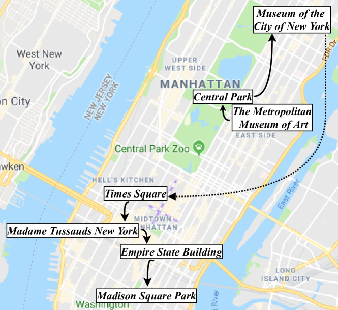
Figure 1: A POI check-in sequence in New York City (dashed line indicates movements across days)

Next POI recommendation is often modeled as a sequential recommendation problem Cheng et al. (2013); Feng et al. (2015, 2017), to take advantage of the sequential patterns in POI visits. For example, tourists at New York City often visit Central Park right after The Metropolitan Museum of Art (“the Met”, cf. Fig. 1). If a user has just checked-in at the Met, Central Park is the next POI to recommend.

Recently, self-attentive networks (SAN) Vaswani et al. (2017), a highly effective and efficient sequence-to-sequence learning model, have been introduced to general sequential recommendation problems. The resultant model named SASRec Kang and Mcauley (2018) yields state-of-the-art performance in recommending next product or video game to purchase, next movie to watch, etc.

Applying SASRec to make next POI recommendations directly, however, may produce sub-optimal results. This is because SASRec is designed for general recommendation scenarios and focuses only on the sequential patterns in the input sequence. It does not consider any spatial or temporal patterns, which are inherent in POI visit sequences and are critical for POI recommendations.

In terms of spatial patterns, as illustrates in Fig. 1, POI visits demonstrate a clustering effect Cheng et al. (2013). POIs nearby have a much larger probability to be visited consecutively than those far away. This offers an important opportunity to alleviate the data sparsity problem resulted from relying only on historical check-in sequences. In an extreme case, we may recommend Central Park to a user at the Met, even if the two POIs had not appeared in the historical check-in sequences, since both POIs are just next to each other and may be visited together.

In terms of temporal patterns, historical check-ins made at different times ago shall have different impact on the next POI visit. For example, in Fig. 1, the solid arrows represent transitions made within the same day, while the dashed arrow represents a transition made across days. Check-ins at Central Park and the Met may have a strong impact on the check-in at Museum of the New York City, as they together form a day trip. In contrast, the check-in at Museum of the New York City may have little impact on the check-in at Times Square, as they are at different days and may well be different trips. SASRec ignores such time differences and just focuses on the transition probabilities between actions (i.e., check-ins). In SASRec, the impact of the check-in at the Met on the check-in at Central Park may be the same as that of the check-in at Museum of the New York City on the check-in at Times Square. Such an impact modeling strategy may be inaccurate for next POI recommendations.

To address these limitations, in this paper, we introduce self-attentive networks to next POI recommendation and integrate spatial and temporal pattern learning into the model. We name our resultant model the SANST model.

To integrate spatial pattern learning, we learn a spatial embedding for each POI and use it as the input of the self-attentive networks. Our embedding preserves the spatial proximity between the POIs, such that the self-attentive networks can learn not only the sequential patterns between the check-ins but also the spatial patterns between the check-ins. To learn our spatial embedding, we first hash the POIs into a grid where nearby cells are encoded by strings with common prefixes (e.g., following a space-filling curve such as the Z-curve). We then learn character embeddings from the hashed strings corresponding to the POIs using Bi-LSTM Hochreiter and Schmidhuber (1997). The Bi-LSTM output is then used as the embedding of the POI. Since POIs at nearby cells are encoded by similar strings, they are expected to obtain similar embeddings in our model. Thus, we preserve the spatial proximity patterns in POI check-ins.

To integrate temporal pattern learning, we follow Shaw et al. (2018) to adapt the attention mechanism. We add a parameter to represent the relative position between two input elements $s^{u}_{i}$ and $s^{u}_{j}$ (i.e., check-ins) in the input sequence. We define the relative position based on the time difference between $s^{u}_{i}$ and $s^{u}_{j}$ instead of the number of other check-ins between $s^{u}_{i}$ and $s^{u}_{j}$ (which was done by Shaw et al. (2018)). This way, our SANST model represents the temporal patterns in check-ins explicitly and can better learn their impact.

To summarize, we make the following contributions:

1. We propose a self-attentive network named SANST that incorporates spatial and temporal POI check-in patterns for next POI recommendation.

2. To incorporate the spatial patterns of POI check-ins, we propose a novel POI embedding technique that preserves the spatial proximity of the POIs. Our technique hashes POIs into a grid where nearby cells are encoded by strings with common prefixes. The POI embeddings are learned from the hashed strings via character embeddings, such that POIs at nearby cells yield similar embeddings.

3. To incorporate the temporal patterns of POI check-ins, we extend the self-attentive network by adding a parameter to represent the relative time between the check-ins. This enables the network to learn the temporal patterns of the check-ins explicitly.

4. We study the empirical performance of our SANST model on three real-world datasets. The results show that SANST outperforms state-of-the-art sequential next POI recommendation models and adapted models that combine self-attentive networks with spatial feature learning directly by up to 13.65% in terms of nDCG@10.

2 Related Work

Like many other recommendation problems, POI recommendation has attracted extensive research interests. Earlier studies on this topic use collaborative filtering (CF) techniques, including both user-based CF (UCF) Ye et al. (2011) and item-based CF (ICF) Levandoski et al. (2012). These techniques make recommendations based on either user or item similarity. Factorization models Gao et al. (2013); Li et al. (2015); Lian et al. (2014) are also widely used, where the user-POI matrix is factorized to learn users’ latent interests towards the POIs. Another stream of studies use probabilistic models Cheng et al. (2012); Kurashima et al. (2013), which aim to model the mutual impact between spatial features and user interests (e.g., via Gaussian or topic models). Details of these studies can be found in a survey Yu and Chen (2015) and an experimental paper Liu et al. (2017).

Next POI recommendation. In this paper, we are interested in a variant of the POI recommendation problem, i.e., next POI recommendation (a.k.a. successive POI recommendation). This variant aims to recommend the very next POI for a user to visit, given the user’s past POI check-in history as a sequence. Users’ sequential check-in patterns play a significant role in this problem. For example, a tensor-based model named FPMC-LR Cheng et al. (2013) recommends the next POI by considering the successive POI check-in relationships. It extends the factorized personalized Markov chain (FPMC) model Rendle et al. (2010) by factorizing the transition probability with users’ movement constraints. Another model named PRME Feng et al. (2015) takes a metric embedding based approach to learn sequential patterns and individual preferences. PRME-G Feng et al. (2015) further incorporates spatial influence using a weight function based on spatial distance. POI2Vec Feng et al. (2017) also makes recommendations based on user and POI embeddings. To learn the embeddings, it adopts the word2vec model Mikolov et al. (2013) originated from the natural language processing (NLP) community; users’ past POI check-in sequences form the “word contexts” for training the word2vec model. The POI check-in time is also an important factor that is considered in next POI recommendation models. For example, STELLAR Zhao et al. (2016) uses ranking-based pairwise tensor factorization to model the interactions among users, POIs, and time. ST-RNN Liu et al. (2016) extends recurrent neural networks (RNN) to incorporate both spatial and temporal features by adding distance-specific and time-specific transition matrices into the model state computation. MTCA Li et al. (2018) and STGN Zhao et al. (2019) adopt LSTM based models to capture the spatio-temporal information. Yuan et al. (2013) split a day into time slots (e.g., by hour) to learn the periodic temporal patterns of POI check-ins. LSTPM Sun et al. (2020) map a week into time slots. They propose a context-aware long and short-term preference modeling framework to model users’ preferences and a geo-dilated RNN to model the non-consecutive geographical relation between POIs.

Attention networks for recommender systems. Due to its high effectiveness and efficiency, the self-attention mechanism Vaswani et al. (2017) has been applied to various tasks such as machine translation. The task of recommendation makes no exception. SASRec Kang and Mcauley (2018) is a sequential recommendation model based on self-attention. It extracts the historical item sequences of each user, and then maps the recommendation problem to a sequence-to-sequence learning problem. AttRec Zhang et al. (2018) uses self-attention to learn from user-item interaction records about their recent interests, which are combined with users’ long term interests learned by a metric learning component to make recommendations. These models have shown promising results in general sequential recommendation problems, e.g., to recommend products, video games, or movies. However, they are not designed for POI recommendations and have not considered the spatio-temporal patterns in POI recommendations. In this paper, we build a self-attentive network based on the SASRec model to incorporate spatio-temporal patterns of user check-ins. We will compare with SASRec in our empirical study. We omit AttRec since SASRec has shown a better result.

Table 1: Frequently Used Symbols

Symbol	Description
$U$	A set of users
$L$	A set of POIs
$T$	A set of check-in time
$S^{u}$	The historical check-in sequence of a user $u$
$s^{u}_{i}$	A historical check-in of a user $u$
$\ell$	The maximum check-in sequence length
$\mathbf{E}$	The input embedding matrix
$r_{l,i}$	A relevant score computed by SASRec

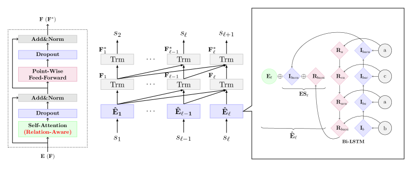
(a) Transformer layer (Trm)                        (b) SASRec model structure                                     (c) Grid cell ID string embedding

Figure 2: The architecture of our SANST model

3 Preliminaries

We start with basic concepts and a problem definition in this section. We then present the SASRec model Kang and Mcauley (2018), based on which our proposed model is built. This model will also be used in our experiments as a baseline. We summarize the frequently used symbols in Table 1.

3.1 Problem Definition

We consider a set of users $U$ and a set of POIs $L$. Each user $u\in U$ comes with a historical POI check-in sequence $S^{u}$ = $\langle s_{1}^{u},s_{2}^{u},...,s_{|S^{u}|}^{u}\rangle$, which is sorted in ascending order of time. Here, $|S^{u}|$ denotes the size of the set $S^{u}$. Every check-in $s_{i}^{u}\in S^{u}$ is a tuple $\langle s_{i}^{u}.l,s_{i}^{u}.t\rangle$, where $s_{i}^{u}.l\in L$ is the check-in POI and $s_{i}^{u}.t$ is the check-in time, respectively.

Given a user $u\in U$ and a time $t_{q}$, our aim is to predict $s_{|S_{u}|+1}^{u}.l\in L$, i.e., the next POI that $u$ will visit at $t_{q}$. In our model, we consider check-in times in the day granularity, to alleviate the data sparsity issue.

3.2 SASRec

SASRec is a two-layer transformer network Vaswani et al. (2017). It models sequential recommendation as a sequence-to-sequence learning problem that translates an input sequence $\langle s_{1},s_{2},...,s_{\ell}\rangle$ to an output sequence $\langle s_{2},s_{3},...,s_{\ell+1}\rangle$. Here, $\ell$ is a hyperparameter controlling the input length. The last element in the output, $s_{\ell+1}$, is the recommendation output. SASRec can be adopted for next POI recommendation directly, by treating a user’s check-in sequence $S^{u}=\langle s^{u}_{1},s^{u}_{2},...,s^{u}_{|S^{u}|}\rangle$ as the model input. If $|S^{u}|>\ell$, only the latest $\ell$ check-ins are kept; if $|S^{u}|<\ell$, the input sequence is padded by 0’s at front.

Fig. 2b illustrates the SASRec model structure. The input sequence of SASRec first goes through an embedding layer to convert every input element $s_{i}$ (e.g., a POI id $s^{u}_{i}.l$) into a $d$-dimensional vector $\mathbf{E_{i}}\in\mathbb{R}^{d}$.

The embeddings are then fed into two stacking transformer layers. In the first transformer layer, as shown in Fig. 2a, the transformer input first goes through a self-attention layer to capture the pairwise dependency between the POI check-ins. Specifically, the embeddings of the input elements are concatenated rowwise to form a matrix $\mathbf{E}=[\mathbf{E_{1}}^{T};\mathbf{E_{2}}^{T};...\mathbf{E_{\ell}}^{T}]^{T}$. Then, three linear projections on $\mathbf{E}$ are done using three projection matrices $\mathbf{W^{Q}},\mathbf{W^{K}},\mathbf{W^{V}}\in\mathbb{R}^{d\times d}$, respectively. These matrices will be learned by the model. The linear projections yield three matrices $\mathbf{Q}=\mathbf{E}\mathbf{W^{Q}}$, $\mathbf{K}=\mathbf{E}\mathbf{W^{K}}$, and $\mathbf{V}=\mathbf{E}\mathbf{W^{V}}$, respectively. The self-attention for $\mathbf{E}$, denoted by $sa(\mathbf{E})$, is then computed as follows, where $\mathbf{Q}$, $\mathbf{K}$, and $\mathbf{V}$ are let be the same:

$$sa(\mathbf{E})=\textrm{softmax}(\frac{\mathbf{QK}^{T}}{\sqrt{d}})\mathbf{V}$$ (1)

To endow the model with non-linearity, a point-wise feed-forward network is applied on $sa(\mathbf{E})$. Let $\mathbf{S_{i}}$ be the $i$-th output of of self-attention module. Then, the feed-forward network on $\mathbf{S_{i}}$ is computed as:

$$\mathbf{F_{i}}=\textrm{ReLU}(\mathbf{S_{i}W}^{(1)}+\mathbf{b}^{(1)})\mathbf{W}^{(2)}+\mathbf{b}^{(2)}$$ (2)

Here, $\mathbf{W}^{(1)},\mathbf{W}^{(2)}\in\mathbb{R}^{d\times d}$ and $\mathbf{b}^{(1)},\mathbf{b}^{(2)}\in\mathbb{R}^{d\times 1}$ are learnable parameters. Layer normalization and dropout are adopted in between these layers to avoid overfitting.

Two transformer layers are stacked to form a deeper network, where the point-wise feed-forward network of the first layer is used as the input as the second layer.

Finally, the prediction output at position $i$ is produced by computing the relevance score $r_{l,i}$ between a POI $l$ and the position-$i$ output $\mathbf{F^{*}_{i}}$ of the point-wise feed-forward network of the second transformer layer.

$$r_{l,i}=\mathbf{F^{*}_{i}}\mathbf{E}(l)^{T}$$ (3)

Here, $\mathbf{E}(l)$ denotes the embedding of $l$ fetched from the embedding layer. The POIs with the highest scores is returned.

To train the model, the binary cross-entropy loss is used as the objective function:

$$-\sum_{u\in U}\sum_{i=1}^{\ell}\Bigg{[}\textrm{log}(\sigma(r_{s^{u}_{i}.l,i}))+\sum_{l\notin S^{u}}\textrm{log}(1-\sigma(r_{l,i}))\Bigg{]}$$ (4)

4 Proposed Model

As discussed earlier, while SASRec can be adapted to make next POI recommendations, a direct adaptation may produce sub-optimal results. This is because SASRec does not consider any spatial or temporal patterns, which are inherent in POI visit sequences and are critical for POI recommendations. In this section, we present our SANST model to address this limitation via incorporating spatial and temporal pattern learning into self-attentive networks. As illustrated in Fig. 2, our SANST model shares the overall structure with SASRec. We detail below how to incorporate spatial and temporal pattern learning into this structure.

4.1 Spatial Pattern Learning

To enable SANST to learn the spatial patterns in POI check-in transitions, we update the embedding $\mathbf{E_{i}}$ of the $i$-th check-in of an input sequence to incorporate the location of the checked-in POI. This way, our SANST model can learn not only the transitions between the POIs (i.e., their IDs) but also the transitions between their locations.

A straightforward approach to incorporate the POI locations is to concatenate the geo-coordinates of the POIs with the SASRec embedding $\mathbf{E_{i}}$. This approach, however, suffers from the data sparsity problem – geo-coordinates of POIs are in an infinite and continuous space, while the number of POIs is usually limited (e.g., thousands).

To overcome the data sparsity, we discritize the data space with a grid such that POI locations are represented by the grid cell IDs. We learn embeddings for the grid cell IDs (detailed next). Then, given a check-in $s^{u}_{i}$, we locate the grid cell in which the check-in POI $s^{u}_{i}.l$ lies. We use the grid cell ID embedding as the spatial embedding of $s^{u}_{i}$, denoted by $\mathbf{ES_{i}}$. We concatenate (denoted by $\oplus$) $\mathbf{ES_{i}}$ with the SASRec embedding $\mathbf{E_{i}}$ to form a new POI embedding in our SANST model, denoted by $\hat{\mathbf{E_{i}}}$:

$$\hat{\mathbf{E_{i}}}=\mathbf{E_{i}}\oplus\mathbf{ES_{i}}$$ (5)

4.1.1 Grid Partitioning and Grid Cell Encoding

We use a space-filling curve to partition the data space and to number the grid cells. We encode the grid cell numbers into strings and use the encoded strings as the grid cell IDs. The purpose is to generate ID strings such that nearby grid cells have similar ID strings. This way, the cell IDs can preserve the spatial proximity of the corresponding cells. We adapt the GeoHash technique to generate the strings as detailed below.

Fig. 3 illustrates the steps of the grid partitioning and grid cell encoding scheme. A Z-curve is used in this figure, although other space-filling curves such as Hilbert-curves may be used as well. Suppose that an order-$n$ curve is used to partition the grid. Then, there are $2^{n}\times 2^{n}$ grid cells, and each curve value is represented by an $2n$-bit integer. We break a curve value into segments of $\gamma$ bits from the left to the right consecutively (a total of $\lceil n/\gamma\rceil$ segments). Each segment is then mapped to a character in a size-$2^{\gamma}$ alphabet. In the figure, we use $\gamma=2$ and an alphabet of $2^{\gamma}=4$ characters (i.e., ‘a’, ‘b’, ‘c’, and ‘d’). As the figure shows, using this encoding, nearby grid cells obtain similar ID strings – they share common prefixes by the definition of the curve values. The longer the common prefix is, the nearer the two cells are. In our experiments, we use $n=60,\gamma=5$, and $\lceil n/\gamma\rceil=12$ .

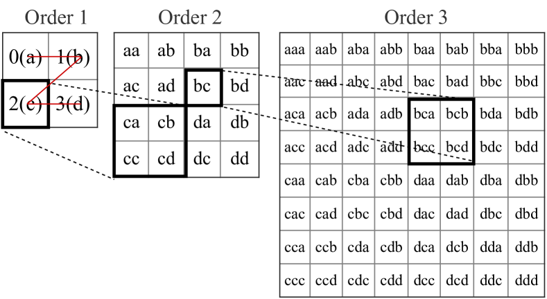
Figure 3: Example of grid cell encoding

4.1.2 Grid Cell ID Embedding Learning

Geohash encodes coordinates in a hierarchical way. It can create adjacent cells without a common prefix, e.g., cells ‘cdb’ and ‘dca’ in Fig. 3. We address this problem by a natural language processing approach – we learn an ID string embedding via learning character embeddings using a Bi-LSTM network. As Fig. 2c shows, each character (a randomly initialized $d_{s}$-dimensional vector to be learned) of an ID string (e.g., “baca”) is fed into Bi-LSTM. The final output of Bi-LSTM in both directions are caught (i.e., $\mathbf{I}_{baca}$ and $\mathbf{R}_{baca}$), which are used as the ID string embedding (i.e., spatial embedding $\mathbf{ES_{i}}$) to form our POI check-in embedding $\hat{\mathbf{E_{i}}}$ in SANST. Since the character embeddings are trained jointly with the entire model, the characters which are adjacent to each other in the grid cells will have similar weights in there embedding vectors. Such as ‘a’ and ‘b’, ‘a’ and ‘c’. Therefore, for the cells labeled with ‘cbd’ and ‘dca’, even though they do not share a common prefix, the adjacency relation between the characters in each layer (e.g., ‘c’ and ‘d’ in the top layer of the hierarchical hash codes) can still be captured. We envision that this spatial embedding method can not only be used in our problem but also other tasks that incorporate spatial information.

4.2 Temporal Pattern Learning

To learn the temporal patterns in POI check-in transitions, we follow Shaw et al. (2018) to adapt the attention mechanism. We add a parameter to represent the relative position between two check-ins $s^{u}_{i}$ and $s^{u}_{j}$ in the input sequence. We define the relative position based on the time difference between $s^{u}_{i}$ and $s^{u}_{j}$ instead of the number of other check-ins between $s^{u}_{i}$ and $s^{u}_{j}$ (which was done by Shaw et al. (2018)). This way, we model the temporal patterns explicitly and can better learn their impact. We detail our adaptation next.

In self-attention, each output element $\mathbf{S_{i}}$ is computed as a weighted sum of linearly transformed input elements, i.e., $\mathbf{S_{i}}=\sum_{j=1}^{\ell}\alpha_{ij}(\mathbf{x_{j}}\mathbf{W^{V}})$, where $\mathbf{x_{j}}$ denotes the position-$i$ input element (e.g., a POI check-in). Shaw et al. (2018) add an edge between two input elements $\mathbf{x_{i}}$ and $\mathbf{x_{j}}$ to model their relative position in the input sequence. The impact of this edge is learned from two vectors $\mathbf{a_{ij}^{V}}$ and $\mathbf{a_{ij}^{K}}$, and the self-attention equation is updated to:

$$\mathbf{S_{i}}=\sum_{j=1}^{\ell}\alpha_{ij}(\mathbf{x_{j}}\mathbf{W^{V}}+\mathbf{a_{ij}^{V}})$$ (6)

Here, $\alpha_{ij}$ is computed as:

$$\alpha_{ij}=\text{softmax}(\frac{\mathbf{x_{i}W^{Q}}(\mathbf{x_{j}W^{K}}+\mathbf{a_{ij}^{K}})^{T}}{\sqrt{d}})$$ (7)

We adapt $\mathbf{a_{ij}^{K}}$ and $\mathbf{a_{ij}^{V}}$ as follows to learn the temporal pattern between $\mathbf{x_{i}}$ and $\mathbf{x_{j}}$ (i.e., the relative position in time):

$$\mathbf{a_{ij}^{K}}=\mathbf{w^{K}_{clip(T_{j}-T_{i},k)}}$$ (8)

$$\mathbf{a_{ij}^{V}}=\mathbf{w^{V}_{clip(T_{j}-T_{i},k)}}$$ (9)

$$clip(x,k)=\max\{-k,\min\{k,x\}\}$$ (10)

Here, $T_{i}$ and $T_{j}$ represent the temporal label on input sequence at position ${i}$ and ${j}$, respectively. We compute the temporal label for the $i$-th input element of user $u$ as $T_{i}=(t_{q}-s_{i}^{u}.t)$. We then learn relative temporal representations $\mathbf{w^{K}}=(\mathbf{w^{K}_{-k}},...,\mathbf{w^{K}_{k}})$ and $\mathbf{w^{V}}=(\mathbf{w^{V}_{-k}},...,\mathbf{w^{V}_{k}})$, where $k$ is a hyperparameter that represents the size of the time context window that we examine. We illustrate these concepts in Fig. 4, where each input element is a user check-in $s_{i}^{u}$.

Figure 4: Temporal pattern learning

4.3 Model Training

We use the same loss function as that of SASRec (i.e., Equation 4) to train SANST. We randomly generate one negative POI for each time step in each sequence in each epoch. The model is optimized by the Adam optimizer.

5 Experiments

We perform an empirical study on the proposed model SANST and compare it with state-of-the-art sequential recommendation and next POI recommendation models.

Table 2: Dataset Statistics

Dataset	$\#$ users	$\#$ POIs	$\#$ check-ins	Time range
Gowalla	10,162	24,250	456,988	02/2009-10/2010
Los Angeles	3,202	4,368	101,327	03/2009-10/2010
Singapore	2,321	5,596	194,108	08/2010-07/2011

Table 3: Summary of Results

	Method	Gowalla		Los Angeles		Singapore
		hit@10	nDCG@10	hit@10	nDCG@10	hit@10	nDCG@10
Baseline	FPMC-LR	0.1197	0.0741	0.2347	0.1587	0.1784	0.1017
	POI2vec	0.0939	0.0606	0.2370	0.1700	0.2063	0.1425
	PRME-G	0.1852	0.1083	0.2367	0.1592	0.1601	0.1049
	SASRec	0.2023	0.1209	0.3648	0.2337	0.2245	0.1429
	SASRec+WF	0.2096	0.1184	0.3304	0.2006	0.2137	0.1251
	SASRec+2KDE	0.1842	0.1113	0.3057	0.1912	0.1900	0.1154
	LSTPM	0.1361	0.0847	0.2366	0.1580	0.1777	0.1105
Variants	SANS	0.2248	0.1372	0.3891	0.2519	0.2417	0.1491
	SANT	0.2028	0.1245	0.3635	0.2264	0.2296	0.1441
Proposed	SANST	0.2273	0.1374	0.3941	0.2558	0.2417	0.1531
		(+8.44%)	(+13.65%)	(+8.03%)	(+9.46%)	(+7.66%)	(+7.14%)

5.1 Settings

We first describe our experimental setup, including datasets, baseline models, and model implementation details.

Datasets. We evaluate the models on three real-world datasets: the Gowalla dataset Yuan et al. (2013), the Los Angeles dataset Cho et al. (2011), and the Singapore dataset Yuan et al. (2013). Table 2 summarizes the dataset statistics. Following previous studies Feng et al. (2015); Cui et al. (2019), for each user’s check-in sequence, we take the last POI for testing and the rest for training, and we omit users with fewer than five check-ins.

Baseline models. We compare with six baseline models:

• FPMC-LR Cheng et al. (2013): This is a matrix factorization model that extends the factorized personalized Markov chain (FPMC) model Rendle et al. (2010) by factorizing the POI transition probability with users’ movement constraints.

• PRME-G Feng et al. (2015): This is a metric embedding based approach to learn sequential patterns and individual preferences, and it incorporates spatial influence using a weight function based on spatial distance.

• POI2Vec Feng et al. (2017): This is an embedding based model. It adopts the word2vec model to compute POI and user embeddings. Recommendations are made based on the embedding similarity.

• LSTPM Sun et al. (2020): This is an LSTM based model. It uses two LSTMs to capture users’ long-term and short-term preferences and a geo-dilated RNN to model the non-consecutive geographical relation between POIs.

• SASRec Kang and Mcauley (2018): This is the state-of-the-art sequential recommendation model as described in the Preliminaries section.

• SASRec+WF: We combine SASRec with spatial pattern learning by adopting a weight function Feng et al. (2015) to weight the relevance score by the spatial distance to the last POI check-in.

• SASRec+2KDE: We combine SASRec with spatial pattern learning by adopting the two-dimensional kernel density estimation (2KDE) model Zhang et al. (2014). The 2KDE model learns a POI check-in distribution for a user based on the POI geo-coordinations. We weight the relevance score for a POI in SASRec by the probability of the POI learned by 2KDE.

Model variants. To study the contribution of the spatial and time pattern learning to the overall performance of SANST, we further compare with two model variants: SANS and SANT, which are SANST without time pattern learning and SANST without spatial pattern learning, respectively.

Implementation details. For FPMC-LR, PRME-G, and POI2Vec, we use the code provided by Cui et al. (2019) (we could not compare with the model proposed by Cui et al. (2019) because they only provided implementations of their baseline models but not their proposed model). For LSTPM, we use the code provided by Sun et al. (2020). For SASRec, we use the code provided by Kang and Mcauley (2018), based on which our SANST model and its variants are implemented. The learning rate, regularization, POI embedding dimensionality, and batch size are set to 0.005, 0.001, 50, and 128 for all models, respectively. Other parameters of the baseline models are set to their default values that come with the original paper. For our SANST model and its variants, we use 2 transformer layers, a dropout rate of 0.3, a character embedding size $d_{s}$ of 20, and the Adam optimizer. We set the maximum POI check-in sequence length $\ell$ to 100, and the time context window size $k$ to be 3, 5 and 1 for Gowalla, Los Angeles and Singapore, respectively. We train the models with an Intel(R) Xeon(R) CPU @ 2.20GHz, a Tesla K80 GPU, and 12GB memory.

We report two metrics: hit@10 and nDCG@10. They measure how likely the ground truth POI is in the top-10 POIs recommended and the rank of the ground truth POI in the top-10 POIs recommended, respectively.

5.2 Results

We first report comparison results with baselines and then report the impact of model components and parameters.

Overall performance. Table 3 summarizes the model performance. We see that our model SANST outperforms all baseline models over all three datasets consistently, in terms of both hit@10 and nDCG@10. The numbers in parentheses show the improvements gained by SANST comparing with the best baselines. We see that SANST achieves up to 8.44% and 13.65% improvements in hit@10 and nDCG@10 (on Gowalla dataset), respectively. These improvements are significant as confirmed by $t$-test with $p<0.05$. Among the baselines, SASRec outperforms FPMC-LR, POI2Vec PRME-G and LSTPM, which validates the effectiveness of self-attentive networks in making next item recommendations. However, adding spatial features to self-attentive networks with existing methods do not necessarily yield a better model. For example, both SASRec+WF and SASRec+2KDE produce worse results than SASRec for most cases tested. They learn spatial patterns and sequential patterns separately which may not model the correlations between the two factors accurately. Our spatial pattern learning technique differs from the existing ones in its ability to learn representations that preserve the spatial information and can be integrated with sequential pattern learning to form an integrated model. Thus, combining self-attentive networks with our spatial pattern learning technique (i.e., SANS) outperforms SASRec, while adding temporal pattern learning (i.e., SANST) further boosts our model performance.

Ablation study. By examining the results of the two model variants SANS and SANT in Table 3, we find that, while both spatial and temporal patterns may help next POI recommendation, spatial patterns appear to contribute more. We conjecture that this is due to the use of the same discretization (i.e., by day) across the check-in time of all users in SANT. Such a global discretization method may not reflect the impact of time for each individual user accurately. It impinges the performance gain achieved from the time patterns. Another observation is that, when both types of patterns are used (i.e., SANST), the model achieves a higher accuracy comparing with using either pattern. This indicates that the two types of patterns complement each other well.

Table 4: Impact of $\ell$ (NDCG@10)

Model	Gowalla		Los Angeles		Singapore
$\ell$	SASRec	SANST	SASRec	SANST	SASRec	SANST
20	0.1131	0.1177	0.2240	0.2369	0.1289	0.1299
50	0.1265	0.1301	0.2326	0.2409	0.1379	0.1431
100	0.1209	0.1374	0.2337	0.2558	0.1429	0.1531
200	0.1251	0.1391	0.2195	0.2355	0.1446	0.1506

Next, we study the impact of hyperparameters and model structure on the performance of SANST. Due to space limit, we only report results on nDCG@10 in these experiments. Results on hit@10 show similar patterns and are omitted.

Impact of input sequence length $\ell$. We start with the impact of the input sequence length $\ell$. As shown in Table 4, SANST outperforms the best baseline SASRec across all $\ell$ values tested. Focusing on our model SANST, as $\ell$ grows from 20 to 100, its nDCG@10 increases. This can be explained by that more information is available for SANST to learn the check-in patterns. When $\ell$ grows further, e.g., to 200, the model performance drops. This is because, on average, the user check-in sequences are much shorter than 200. Forcing a large input length requires padding 0’s at front which do not contribute extra information. Meanwhile, looking too far back may introduce noisy check-in patterns. Thus, a longer input sequence may not benefit the model.

Impact of character embedding dimensionality $d_{s}$. We vary the character embedding dimensionality $d_{s}$ for our spatial pattern learning module from 10 to 30 and report the performance of SANST in Fig. 5a. As the figure shows, our model is robust against the character embedding dimensionality (note the small value range in the $y$-axis. When $d_{s}=20$, the model has the best overall performance across the datasets. This relates to the fact that the size of the character vocabulary used to generate the location hashing strings is 32. If $d_{s}$ is much smaller than 32, the character embedding may not capture sufficient information from the hashing strings. Meanwhile, if $d_{s}$ is too large, the information captured by each dimension may become too weak due to data sparsity. Another observation is that the model performs much better on Los Angeles. This is because Los Angeles has the smallest number of POIs and average check-in sequence length per user. Its data space to be learned is smaller than those of the other two datasets.

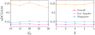
(a) Character embedding size  (b) Time window size

Figure 5: Impact of character embedding size $d_{S}$ and time context window size $k$

Impact of time context window size $k$. We vary the time context window size $k$ for our temporal pattern learning module from 1 to 5 and report the results in Fig. 5b. We see that SANST is also robust against the time context window size. We find the best time context window size to be strongly correlated to the time span and the average length of the check-in sequences in a dataset. In particular, Los Angeles covers a long time span (20 months) while its average check-in sequence length is the shortest. This means that its check-ins are less dense in the time dimension. Thus, it needs a larger time context window to achieve better performance, which explains for its increasing trend in nDCG@10 as $k$ increases towards 5.

Impact of model structure. The transformer network can be stacked with multiple layers, while the attention network can have multi-heads. We show the impact of the number of transformer network layers $\tau$ and the number of heads $h$ in Table 5. We see better results on Los Angeles with $\tau=2$, i.e., two transformer layers, which demonstrates that a deeper self-attention network may be helpful for learning the data patterns. However, deeper networks also have the tendency to overfit. The model performance drops when $\tau=2$ on the other two datasets. When $\tau=3$, the model is worse on all three datasets. We keep $\tau=2$ and further add more heads to the attention network. As the table shows, adding more heads does not help the model performance. This is opposed to observations in natural language processing tasks where different attention heads are more effective to capture various type of relations (e.g., positional and syntactic dependency relations) Voita et al. (2019). We conjecture that the relations between POIs are simpler (and without ambiguity) than those between words in natural language. Thus, a single-head attention is sufficient for our task.

Table 5: Impact of Model Structure (NDCG@10)

Structure	Gowalla	Los Angeles	Singapore
$\tau$=1, $h$=1	0.1426	0.2462	0.1539
$\tau$=2, $h$=1 (default)	0.1374	0.2558	0.1531
$\tau$=3, $h$=1	0.1278	0.2416	0.1464
$\tau$=2, $h$=2	0.1358	0.2516	0.1464

6 Conclusions

We studied the next POI recommendation problem and proposed a self-attentive network named SANST for the problem. Our SANST model takes advantage of self-attentive networks for their capability in making sequential recommendations. Our SANST model also incorporates the spatial and temporal patterns of user check-ins. As a result, SANST retains the high efficiency of self-attentive networks while enhancing their power in making recommendations for next POI visits. Experimental results on real-world datasets confirm the superiority of SANST – it outperforms state-of-the-art sequential recommendation models and adapted baseline models that combine self-attentive networks with spatial features directly by up to 13.65% in nDCG@10.

References

- Cheng et al. [2012] Chen Cheng, Haiqin Yang, Irwin King, and Michael R Lyu. Fused matrix factorization with geographical and social influence in location-based social networks. In AAAI Conference on Artificial Intelligence (AAAI), pages 17–23, 2012.
- Cheng et al. [2013] Chen Cheng, Haiqin Yang, Michael R Lyu, and Irwin King. Where you like to go next: Successive point-of-interest recommendation. In International Joint Conference on Artificial Intelligence (IJCAI), pages 2605–2611, 2013.
- Cho et al. [2011] Eunjoon Cho, Seth A Myers, and Jure Leskovec. Friendship and mobility: user movement in location-based social networks. In ACM SIGKDD International Conference on Knowledge Discovery and Data Mining (KDD), pages 1082–1090, 2011.
- Cui et al. [2019] Qiang Cui, Yuyuan Tang, Shu Wu, and Liang Wang. Distance2pre: Personalized spatial preference for next point-of-interest prediction. In Pacific-Asia Conference on Knowledge Discovery and Data Mining (PAKDD), pages 289–301, 2019.
- Feng et al. [2015] Shanshan Feng, Xutao Li, Yifeng Zeng, Gao Cong, Yeow Meng Chee, and Quan Yuan. Personalized ranking metric embedding for next new poi recommendation. In International Joint Conference on Artificial Intelligence (IJCAI), pages 2069–2075, 2015.
- Feng et al. [2017] Shanshan Feng, Gao Cong, Bo An, and Yeow Meng Chee. Poi2vec: Geographical latent representation for predicting future visitors. In AAAI Conference on Artificial Intelligence (AAAI), pages 102–108, 2017.
- Gao et al. [2013] Huiji Gao, Jiliang Tang, Xia Hu, and Huan Liu. Exploring temporal effects for location recommendation on location-based social networks. In ACM Conference on Recommender systems (RecSys), pages 93–100, 2013.
- Hochreiter and Schmidhuber [1997] Sepp Hochreiter and Jürgen Schmidhuber. Long short-term memory. Neural Computation, 9(8):1735–1780, 1997.
- Kang and Mcauley [2018] Wang Cheng Kang and Julian Mcauley. Self-attentive sequential recommendation. In IEEE International Conference on Data Mining (ICDM), pages 197–206, 2018.
- Kurashima et al. [2013] Takeshi Kurashima, Tomoharu Iwata, Takahide Hoshide, Noriko Takaya, and Ko Fujimura. Geo topic model: joint modeling of user’s activity area and interests for location recommendation. In ACM International Conference on Web Search and Data Mining (WSDM), pages 375–384, 2013.
- Levandoski et al. [2012] Justin J Levandoski, Mohamed Sarwat, Ahmed Eldawy, and Mohamed F Mokbel. Lars: A location-aware recommender system. In IEEE International Conference on Data Engineering (ICDE), pages 450–461, 2012.
- Li et al. [2015] Xutao Li, Gao Cong, Xiao-Li Li, Tuan-Anh Nguyen Pham, and Shonali Krishnaswamy. Rank-geofm: A ranking based geographical factorization method for point of interest recommendation. In ACM SIGIR Conference on Information Retrieval (SIGIR), pages 433–442, 2015.
- Li et al. [2018] Ranzhen Li, Yanyan Shen, and Yanmin Zhu. Next point-of-interest recommendation with temporal and multi-level context attention. In 2018 IEEE International Conference on Data Mining (ICDM), pages 1110–1115. IEEE, 2018.
- Lian et al. [2014] Defu Lian, Cong Zhao, Xing Xie, Guangzhong Sun, Enhong Chen, and Yong Rui. Geomf: Joint geographical modeling and matrix factorization for point-of-interest recommendation. In ACM SIGKDD International Conference on Knowledge Discovery and Data Mining (KDD), pages 831–840, 2014.
- Liu et al. [2016] Qiang Liu, Shu Wu, Liang Wang, and Tieniu Tan. Predicting the next location: A recurrent model with spatial and temporal contexts. In AAAI Conference on Artificial Intelligence (AAAI), pages 194–200, 2016.
- Liu et al. [2017] Yiding Liu, Tuan-Anh Nguyen Pham, Gao Cong, and Quan Yuan. An experimental evaluation of point-of-interest recommendation in location-based social networks. Proceedings of the VLDB Endowment, 10(10):1010–1021, 2017.
- Mikolov et al. [2013] Tomas Mikolov, Kai Chen, Greg Corrado, and Jeffrey Dean. Efficient estimation of word representations in vector space. In International Conference on Learning Representations Workshops, 2013.
- Rendle et al. [2010] Steffen Rendle, Christoph Freudenthaler, and Lars Schmidt-Thieme. Factorizing personalized markov chains for next-basket recommendation. In International Conference on World Wide Web (WWW), pages 811–820, 2010.
- Shaw et al. [2018] Peter Shaw, Jakob Uszkoreit, and Ashish Vaswani. Self-attention with relative position representations. arXiv preprint arXiv:1803.02155, 2018.
- Statista [2018] Statista. Global travel and tourism industry - Statistics & Facts. https://www.statista.com/topics/962/global-tourism/, 2018.
- Sun et al. [2020] Ke Sun, Tieyun Qian, Tong Chen, Yile Liang, Quoc Viet Hung Nguyen, and Hongzhi Yin. Where to Go Next: Modeling Long-and Short-Term User Preferences for Point-of-Interest Recommendation. In AAAI Conference on Artificial Intelligence (AAAI), page To appear, 2020.
- Vaswani et al. [2017] Ashish Vaswani, Noam Shazeer, Niki Parmar, Jakob Uszkoreit, Llion Jones, Aidan N Gomez, Łukasz Kaiser, and Illia Polosukhin. Attention is all you need. In Advances in Neural Information Processing Systems (NeurIPS), pages 5998–6008, 2017.
- Voita et al. [2019] Elena Voita, David Talbot, Fedor Moiseev, Rico Sennrich, and Ivan Titov. Analyzing multi-head self-attention: Specialized heads do the heavy lifting, the rest can be pruned. In Annual Meeting of the Association for Computational Linguistics, pages 5797–5808, 2019.
- Ye et al. [2011] Mao Ye, Peifeng Yin, Wang-Chien Lee, and Dik-Lun Lee. Exploiting geographical influence for collaborative point-of-interest recommendation. In ACM SIGIR Conference on Information Retrieval (SIGIR), pages 325–334, 2011.
- Yu and Chen [2015] Yonghong Yu and Xingguo Chen. A survey of point-of-interest recommendation in location-based social networks. In Workshops at the AAAI Conference on Artificial Intelligence, pages 53–60, 2015.
- Yuan et al. [2013] Quan Yuan, Gao Cong, Zongyang Ma, Aixin Sun, and Nadia Magnenat Thalmann. Time-aware point-of-interest recommendation. In ACM SIGIR Conference on Information Retrieval (SIGIR), pages 363–372, 2013.
- Zhang et al. [2014] Jia-Dong Zhang, Chi-Yin Chow, and Yanhua Li. Lore: Exploiting sequential influence for location recommendations. In ACM SIGSPATIAL International Conference on Advances in Geographic Information Systems, pages 103–112, 2014.
- Zhang et al. [2018] Shuai Zhang, Yi Tay, Lina Yao, and Aixin Sun. Next item recommendation with self-attention. arXiv preprint arXiv:1808.06414, 2018.
- Zhao et al. [2016] Shenglin Zhao, Tong Zhao, Haiqin Yang, Michael R Lyu, and Irwin King. Stellar: spatial-temporal latent ranking for successive point-of-interest recommendation. In AAAI conference on artificial intelligence (AAAI), pages 315–321, 2016.
- Zhao et al. [2019] Pengpeng Zhao, Haifeng Zhu, Yanchi Liu, Jiajie Xu, Zhixu Li, Fuzhen Zhuang, Victor S Sheng, and Xiaofang Zhou. Where to go next: A spatio-temporal gated network for next poi recommendation. In Proceedings of the AAAI Conference on Artificial Intelligence, volume 33, pages 5877–5884, 2019.