Saddlepoint approximations for
spatial panel data models

Abstract

We develop new higher-order asymptotic techniques for the Gaussian maximum likelihood estimator in a spatial panel data model, with fixed effects, time-varying covariates, and spatially correlated errors. Our saddlepoint density and tail area approximation feature relative error of order $O(1/(n(T-1)))$ with $n$ being the cross-sectional dimension and $T$ the time-series dimension. The main theoretical tool is the tilted-Edgeworth technique in a non-identically distributed setting. The density approximation is always non-negative, does not need resampling, and is accurate in the tails. Monte Carlo experiments on density approximation and testing in the presence of nuisance parameters illustrate the good performance of our approximation over first-order asymptotics and Edgeworth expansions. An empirical application to the investment-saving relationship in OECD (Organisation for Economic Co-operation and Development) countries shows disagreement between testing results based on first-order asymptotics and saddlepoint techniques.

Keywords: Higher-order asymptotics, investment-saving, random field, tail area.

1 Introduction

Accounting for spatial dependence is of interest both from an applied and a theoretical point of view. Indeed, panel data with spatial cross-sectional interaction enable empirical researchers to take into account the temporal dimension and, at the same time, control for the spatial dependence. From a theoretical point of view, the special features of panel data with spatial effects present the challenge to develop new methodological tools.

Much of the machinery for conducting statistical inference on panel data models has been established under the simplifying assumption of cross-sectional independence. This assumption may be inadequate in many cases. For instance, correlation across spatial data comes typically from competition, spillovers, or aggregation. The presence of such a correlation might be anticipated in observable variables and/or in the unobserved disturbances in a statistical model and ignoring it can have adverse effects on routinely-applied inferential procedures. See, e.g., Gaetan and Guyon, (2010), Rosenblatt, (2012), Cressie, (2015), Cressie and Wikle, (2015), and recently Wikle et al., (2019) for book-length discussions in the statistical literature. In the econometric literature, see, e.g., Kapoor et al., (2007), Lee and Yu, (2010), Robinson and Rossi, 2014b , Robinson and Rossi, (2015), and, for book-length presentations, Baltagi, (2008, Ch. 13), Anselin, (1988), and Kelejian and Piras, (2017).

Different nonparametric, semiparametric, and parametric approaches have been proposed to incorporate cross-sectional dependence in panel data models. The choice on the modeling approach depends on the time series ($T$) and cross-sectional ($n$) dimensions. A nonparametric approach is only feasible when $T$ is large relative to $n$. In other situations, typically when $T$ is very small (e.g., $T=2$) and $n$ is large, semiparametric models have been employed, including time varying regressors (namely factor models) and spatial autoregressive component, when information on spatial distances is available. Least squares and quasi maximum-likelihood estimator represent the main popular tools for estimation within this setting. When both $T$ and $n$ are small, the parametric approach is the sensible choice and (Gaussian) likelihood-based procedures are applied to define the maximum likelihood estimator (MLE).

There is a vast literature on the MLE for spatial autoregressive models, an early reference being Ord, (1975). The derivation of the first-order asymptotics is available in the econometric literature; we refer to the seminal paper by Lee, (2004). For the class of spatial autoregressive processes, with fixed effects, time-varying covariates, and spatially correlated errors that we consider in this paper, the first-order asymptotic results for the Gaussian MLE are available in Lee and Yu, (2010), where the authors derive asymptotic approximations (the exact finite-sample distribution being intractable), when the cross-sectional dimension $n$ is large and $T$ is finite or large.

The main issue related to first-order asymptotic approximations is that, when $n$ is not very large, such approximations may be unreliable: alternatives are highly recommended. Bao and Ullah, (2007) provide analytic formulae for the second-order bias and mean squared error of the MLE for the spatial parameter $\lambda$, in a Gaussian model. Bao, (2013) and Yang, (2015) extend these approximations to include also exogenous explanatory variables, which remain valid also when the process is not Gaussian. Robinson and Rossi, 2014a ; Robinson and Rossi, 2014b develop Edgeworth-improved tests for no spatial correlation in spatial autoregressive models for pure cross-sectional data based on least squares estimation and Lagrange multiplier tests. Moreover, Robinson and Rossi, (2015) work on the concentrated likelihood and derive an Edgeworth expansion for MLE of $\lambda$ in the setting of a first-order spatial autoregressive panel data model, with fixed effects and without covariates. Hillier and Martellosio, (2018) (see their §6) and Martellosio and Hillier, (2020) (see their §3.5) propose saddlepoint approximations for the profile likelihood estimator of $\lambda$.

Resampling methods are also available alternatives to improve on the first-order asymptotics, achieving higher-order asymptotic refinements in terms of absolute error. However, it requires either a bias correction or an asymptotically pivotal statistics; see Hall, (1992) and Horowitz, (2001) in the i.i.d. setting. To the best of our knowledge, for spatial panel models considered in this paper, such results are not available.

The aim of this paper is to introduce saddlepoint approximations for parametric spatial autoregressive panel data models with fixed effects and time-varying covariates. They overcome the problems mentioned above by means of the tilted-Edgeworth technique. For general references on saddlepoint approximations in the i.i.d. setting, see the seminal paper of Daniels, (1954) and the book-length presentations of Field and Ronchetti, (1990), Jensen, (1995), Kolassa, (2006), and Brazzale et al., (2007). For a result about testing on spatial dependence, see Tiefelsdorf, (2002), and for developments in time series models, see La Vecchia and Ronchetti, (2019).

We remark that we could cast the methodology of this paper into the framework of statistical analysis of random fields on a network graph, where the underlying, known, network graph describes the spatial structure of the stochastic process; see e.g. Kolaczyk, (2009) Ch. 8 for a book-length introduction. In §2, we briefly comment on this approach. For the ease-of-reference to the extant econometric literature, in the rest of the paper, we prefer to stick to the econometric notation and terminology of spatial panel data models.

The paper is organized as follows. In §2, we provide a motivating example. §3 defines the general model setting and the estimation method, whereas the detailed methodology is presented in §4. In particular in §4.5 we provide a detailed discussion about the connections with the econometric literature. Algorithms and computational aspects are discussed in §5. §6 provides numerical comparison with other methods and, in §6.2, we tackle the problem of testing in the presence of nuisance parameters. In §7, we present an empirical application. The online Supplementary Material contains detailed derivations, technical appendices and additional numerical experiments.

2 Motivating example

We motivate our research by a Monte Carlo (MC) exercise illustrating the low accuracy of the routinely applied first-order asymptotics in the setting of spatial panel data model. We consider the model:

$$Y_{nt} =\lambda_{0}W_{n}Y_{nt}+X_{nt}\beta_{0}+c_{n0}+E_{nt},$$ (2.1)

$$E_{nt} =\rho_{0}M_{n}E_{nt}+V_{nt}, \quad t=1,....,T,$$

where $Y_{nt}=(y_{1t},y_{2t},...,y_{nt})$, $X_{nt}$ is an $n\times k$ matrix of non stochastic time-varying regressors, $c_{n0}$ is an $n\times 1$ vector of fixed effects, and $V_{nt}=(v_{1t},v_{2t},..,v_{nt})^{\prime}$ are $n\times 1$ vectors with $v_{it}\sim\mathcal{N}(0,\sigma_{0}^{2})$, i.i.d. across $i$ and $t$. The matrices $W_{n}$ and $M_{n}$ are weighting matrices describing the spatial dynamics. Following the literature, we label this model SARAR(1,1) to emphasize the spatial dependence in both the response variable $Y_{nt}$ and the error $E_{nt}$.

As in the MC example in Lee and Yu, (2010) p. 172, we generate samples from (2.1) using $\theta_{0}=(\beta_{0},\lambda_{0},\rho_{0},\sigma_{0}^{2})^{\prime}=(1.0,0.2,0.5,1)^{\prime}$, $T=5$, and $k=4$ covariates. The quantities $X_{nt}$, $c_{n0}$ and $V_{nt}$ are generated from independent standard normal distributions and, as it is customary in the econometric literature, we set $W_{n}=M_{n}$, where the off-diagonal elements are different from zero, while the diagonal elements are all zero. We consider two sample sizes: $n=24$ (small sample) and $n=100$ (moderate/large sample). The choice of $n=24$ is related to the empirical data analysis that we consider in §7, where we apply the model in (2.1) to conduct inference on the investment-saving relation for the 24 OECD (Organisation for Economic Co-operation and Development) countries. Similar sample sizes arise in many real data analyses, where panel datasets contain a limited number of cross-sectional units, e.g., sampling can be expensive and/or time consuming, as it is typically the case in field studies.

As it is customary in the statistical/econometric software, we illustrate the inference issues related to the use of the first-order asymptotics by means of three different spatial weight matrices: Rook matrix, Queen matrix, and Queen matrix with torus. In Figure 1, we display the geometry of $Y_{nt}$ as implied by each considered spatial matrix: the plots highlight that different matrices imply different spatial relations. For instance, we see that the Rook matrix implies fewer links than the Queen matrix. Indeed, the Rook criterion defines neighbours by the existence of a common edge between two spatial units, whilst the Queen criterion is less rigid and defines neighbours as spatial units sharing an edge or a vertex. Besides, we may interpret $\{Y_{nt}\}$ as a $n$-dimensional random field on the network graph which describes the known underlying spatial structure. Then, $W_{n}$ represents the weighted adjacency matrix (in the spatial econometrics literature, $W_{n}$ is called contiguity matrix). In Figure 1, we display the geometry of a random field on a regular lattice (undirected graph). In the real data example of §7, we consider a random field over a manifold (a sphere), providing two additional examples for $W_{n}$.

Rook                                  Queen                                   Queen torus

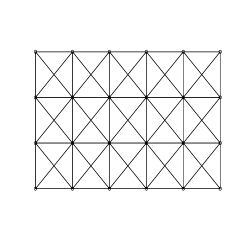
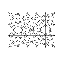
Figure 1: Different types of neighboring structure for $Y_{nt}$, as implied by different types of $W_{n}$ matrix, for $n=24$.

To illustrate the inferential issues entailed by the use of first-order asymptotics, for each type of $W_{n}$, we generate a sample of $n$ observations. Since $c_{n0}$ creates an incidental parameter issue, we eliminate it by the standard differentiation procedure, and for each MC run we estimate the model parameter $\theta$ using the transformation approach of Lee and Yu, (2010), with maximum likelihood estimation method; we refer to the R package spml for implementation details. We set the MC size to 5000.

We illustrate graphically the behavior of the first-order asymptotic theory in finite sample by comparing the distribution of $\hat{\lambda}$ to the Gaussian asymptotic distribution (see §4.1 for details). Via QQ-plot analysis, Figure 2 shows that the Gaussian approximation can be either too thin or too thick in the tails with respect to the “exact” distribution. For instance, when $n=24$ and $W_{n}$ is rook, the Gaussian quantiles are larger than the “exact” ones in the left tail, while we observe the opposite phenomenon in the right tail. Similar considerations hold for the other types of $W_{n}$. The more complex is the geometry of $W_{n}$ (e.g., $W_{n}$ has Queen structure) the more pronounced are the departures from the Gaussian. For $n=100$, and $W_{n}$ Rook, the MLE displays a distribution which is in line with the Gaussian one (see bottom left panel). However, when $W_{n}$ becomes more complex (e.g., Queen with torus), larger departures in the tails are still evident. In Appendix D.1, we illustrate that similar conclusions are available also for the simpler SAR(1) model:

$$Y_{nt} = \lambda_{0}W_{n}Y_{nt}+c_{n0}+V_{nt},\quad{\text{for}}\quad t=1,2,$$ (2.2)

where $\theta_{0}=(\lambda_{0},\sigma_{0}^{2})^{\prime}$. More generally, unreported results suggest that, in the considered SARAR setting, the “exact” and the asymptotic distribution, as well as the saddlepoint approximation, agree for the considered types of $W_{n}$, when $n\geq 250$.

Rook                             Queen                   Queen torus

$n=24$

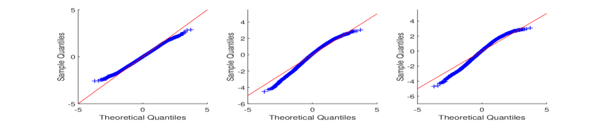
$n=100$

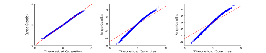
Figure 2: SARAR(1,1) model: QQ-plot vs normal of the MLE $\hat{\lambda}$, for different sample sizes ($n=24$ and $n=100$), $\lambda_{0}=0.2$, and different types of $W_{n}$ matrix.

3 Model setting and estimation method

Let us consider a random field described by the SARAR(1,1) model in (2.1). We label by $P_{\theta_{0}}\in\mathcal{P}$, with $\theta_{0}\in\Theta\subset\mathbb{R}^{d}$, the actual underlying distribution, which is characterized by $\theta_{0}=(\beta_{0},\lambda_{0},\rho_{0},\sigma_{0}^{2})^{\prime}$, the true parameter value. The matrix $W_{n}$ is an $n\times n$ nonstochastic spatial weight matrix that generates the spatial dependence on $y_{it}$ among cross sectional units. The matrix $X_{nt}$ is an $n\times k$ matrix of non stochastic time varying regressors, and $c_{n0}$ is an $n\times 1$ vector of fixed effects. Similarly, $M_{n}$ is an $n\times n$ spatial weight matrix for the disturbances — quite often $W_{n}=M_{n}$. Moreover, we define $S_{n}(\lambda)=I_{n}-\lambda W_{n}$, and analogously $R_{n}(\rho)=I_{n}-\rho M_{n}$.

The vector $c_{n0}$ introduces an incidental parameter problem; see Lee and Yu, (2010) and Robinson and Rossi, (2015). To cope with this issue, we follow the standard approach, and we transform the model in order to derive consistent estimator for the model parameter $\theta=(\beta^{\prime},\lambda,\rho,\sigma^{2})^{\prime}$ and $\theta\in\Theta\subset\mathbb{R}^{d}$. To achieve the goal, we first eliminate the individual effects by the deviation from the time-mean operator $J_{T}=(I_{T}-\frac{1}{T}l_{T}l^{\prime}_{T})$, where $I_{T}$ is the $T\times T$ identity matrix, and $l_{T}=(1,...,1)^{\prime}$, namely the $T\times 1$ vector of ones. Without creating linear dependence in the resulting disturbances, we adopt the transformation introduced by Lee and Yu, (2010).

First, let the orthonormal eigenvector matrix of $J_{T}$ be $[F_{T,T-1},\frac{1}{\sqrt{T}}l_{T}]$, where $[\cdot]$ represents a matrix horizontal concatenation and $F_{T,T-1}$ is the $T\times(T-1)$ submatrix corresponding to the unit eigenvalues. Then, for any $n\times T$ matrix $[Z_{n1},...,Z_{nT}]$, we define the transformed $n\times(T-1)$ matrix $[Z^{*}_{n1},...,Z^{*}_{nT}]=[Z_{n1},...,Z_{nT}]F_{T,T-1}.$ Similarly, we define $X^{*}_{nt}=[X^{*}_{nt,1},X^{*}_{nt,2},...,X^{*}_{nt,k}]$. Thus, we transform the model in (2.1) and we obtain:

$$Y^{*}_{nt} =\lambda_{0}W_{n}Y^{*}_{nt}+X^{*}_{nt}\beta_{0}+E^{*}_{nt},$$ (3.1)

$$E^{*}_{nt} =\rho_{0}M_{n}E^{*}_{nt}+V^{*}_{nt}, \quad t=1,2,...,T.$$

Since $\left(V^{*^{\prime}}_{n1},...,V^{*^{\prime}}_{n(T-1)}\right)^{\prime}=\left(F^{\prime}_{T,T-1}\otimes I_{n}\right)\left(V^{\prime}_{n1},...,V^{\prime}_{n(T-1)}\right)^{\prime},$ and the $v_{it}$ are i.i.d., we have

$$\mathbb{E}\left[\left(V^{*^{\prime}}_{n1},...,V^{*^{\prime}}_{n(T-1)}\right)^{\prime}\left(V^{*^{\prime}}_{n1},...,V^{*^{\prime}}_{n(T-1)}\right)\right]=\sigma_{0}^{2}I_{n(T-1)},$$

where $\mathbb{E}[\cdot]$ represents the expectation taken w.r.t. $P_{\theta_{0}}$. Now, the Gaussian assumption on the innovation terms implies that $v^{*}_{it}$ are independent for all $i$ and $t$; without this assumption, they would be simply uncorrelated. See Lee and Yu, (2010) p. 167. Thus, defining $\zeta=(\beta^{\prime},\lambda,\rho)^{\prime}$, the log-likelihood is:

$$\ln L_{n,T}(\theta)=\ell_{n,T}(\theta) = -\frac{n(T-1)}{2}\ln(2\pi\sigma^{2})+(T-1)[\ln|S_{n}(\lambda)|+\ln|R_{n}(\rho)|]$$

$$\qquad-\frac{1}{2\sigma^{2}}\sum_{t=1}^{T-1}V^{*^{\prime}}_{nt}(\zeta)V^{*}_{nt}(\zeta),$$

where $V^{*}_{nt}(\zeta)=R_{n}(\rho)[S_{n}(\lambda)Y^{*}_{nt}-X^{*}_{nt}\beta].$ As remarked in Lee and Yu, (2010), the function $L_{n,T}$ has a conditional likelihood interpretation: it is the likelihood conditional on the time average $\sum_{t=1}^{T}Y_{nt}/T$, which is a sufficient statistic for $c_{n0}$, under normality.

We rewrite $\ell_{n,T}(\theta)$ in terms of a quadratic form in $\tilde{V}_{nt}(\zeta)$ as:

$$\ell_{n,T}(\theta) = -\frac{n(T-1)}{2}\ln(2\pi\sigma^{2})+(T-1)[\ln|S_{n}(\lambda)|+\ln|R_{n}(\rho)|]$$ (3.2)

$$-\qquad\frac{1}{2\sigma^{2}}\sum_{t=1}^{T}\tilde{V}^{\prime}_{nt}(\zeta)\tilde{V}_{nt}(\zeta),$$

where $\tilde{V}_{nt}(\zeta)=R_{n}(\rho)[S_{n}(\lambda)\tilde{Y}_{nt}-\tilde{X}_{nt}\beta],$ with

$$\tilde{Y}_{nt}={Y}_{nt}-\sum_{t=1}^{T}Y_{nt}/T,\quad\tilde{X}_{nt}=X_{nt}-\sum_{t=1}^{T}X_{nt}/T.$$ (3.3)

The MLE $\hat{\theta}_{n,T}$ for $\theta$ is an $M$-estimator obtained by solving $\hat{\theta}_{n,T}=\text{arg}\max_{\theta\in\Theta}\ell_{n,T}(\theta).$ It implies the system of estimating equations:

$$0=\frac{\partial\ell_{n,T}(\hat{\theta}_{n,T})}{\partial{\theta}}=\sum_{t=1}^{T}(T-1)^{-1}\psi_{nt}(\hat{\theta}_{n,T}),$$ (3.4)

where $\psi_{nt}$ is the likelihood score function

$$\psi_{nt}(\theta)=\left(\begin{array}[]{cc}\frac{T-1}{\sigma^{2}}(R_{n}(\rho)\tilde{X}_{nt})^{\prime}\tilde{V}_{nt}(\zeta)\\ \frac{T-1}{\sigma^{2}}\left(\left(\ddot{G}_{n}\ddot{X}_{nt}\beta\right)^{\prime}\tilde{V}_{nt}(\zeta)+\tilde{V}_{nt}^{{}^{\prime}}\ddot{G}_{n}^{{}^{\prime}}\tilde{V}_{nt}\right)-\frac{(T-1)^{2}}{T}\text{tr}({G}_{n}(\lambda))\\ \frac{T-1}{\sigma^{2}}(H_{n}(\rho)\tilde{V}_{nt}(\zeta))^{\prime}\tilde{V}_{nt}(\zeta)-\frac{(T-1)^{2}}{T}\text{tr}(H_{n}(\rho))\\ \frac{T-1}{2\sigma^{4}}\left(\tilde{V}^{\prime}_{nt}(\zeta)\tilde{V}_{nt}(\zeta)-\frac{n(T-1)}{T}\sigma^{2}\right)\end{array}\right),$$ (3.5)

where $G_{n}(\lambda)=W_{n}S_{n}^{-1},\quad H_{n}(\rho)=M_{n}R_{n}^{-1},\quad\ddot{G}_{n}(\lambda)=R_{n}G_{n}R_{n}^{-1}$, and $\ddot{X}_{nt}=R_{n}\tilde{X}_{nt}.$

4 Methodology

We assume $n\gg T$, so we deal with so-called micro panels: in the econometric literature, this type of data typically involve annual records covering a short time span for each individual. Within this setting for $T$ being fixed, the standard asymptotic arguments rely crucially on the number $n$ of individuals tending to infinity; see Lee and Yu, (2010). In contrast, in our development, we consider small sample cross-sectional asymptotics (Field and Ronchetti, (1990)), and we still leave $T$ fixed (possibly small). However, we will keep $T$ in the notation of normalizing factors to demonstrate the improved rate of convergence that would result if $T\to\infty$ or it is large. The derivation of our higher-order techniques relies on three steps: (i) defining a second-order asymptotic (von Mises) expansion for the MLE, see §4.1; (ii) identifying the corresponding $U$-statistic, see §4.2; (iii) deriving the Edgeworth expansion for the $U$-statistic as in Bickel et al., (1986) and deriving the saddlepoint density by means of the tilted-Edgeworth technique, see §4.3 and §4.4. Similar approaches are available in the standard setting of i.i.d. random variables in Easton and Ronchetti, (1986), Barndorff-Nielsen and Cox, (1989), and Gatto and Ronchetti, (1996).

4.1 The $M$-functional related to the MLE and its first-order asymptotics

Let us first define the $M$-functional related to the MLE. To this end, we remark that the likelihood score function in (3.5) is a vector in $\mathbb{R}^{d}$, and each $l$-th element of this vector, for $l=1,...,d$, is a sum of $n$ terms. In what follows, for $i=1,...,n$, we denote by $\psi_{i,t,l}(\theta)$ the $i$-th term, at time $t$, of this sum for the $l$-th component of the score.

To specify $\psi_{i,t,l}(\theta)$, we set $R_{n}(\rho)=\left(r_{1}^{{}^{\prime}}(\rho),r_{2}^{{}^{\prime}}(\rho),\cdots,r_{n}^{{}^{\prime}}(\rho)\right)^{\prime},$

$$\tilde{X}_{nt}=\left[\tilde{X}_{nt,1},\tilde{X}_{nt,2},\cdots,\tilde{X}_{nt,k}\right],$$

$\tilde{V}_{nt}(\zeta)=\left(\tilde{v}_{1t}(\zeta),\tilde{v}_{2t}(\zeta),\cdots,\tilde{v}_{nt}(\zeta)\right)^{\prime}$ and $H_{n}(\rho)=\left(h_{1}^{{}^{\prime}}(\rho),h_{2}^{{}^{\prime}}(\rho),\cdots,h_{n}^{{}^{\prime}}(\rho)\right)^{\prime}$, where $r_{i}(\rho)$ and $h_{i}(\rho)$ are the $i_{th}$ row of $R_{n}(\rho)$ and $H_{n}(\rho)$, $g_{ii}$ and $h_{ii}$ are $i_{th}$ element of the diagonal of $G_{n}(\lambda)$ and $H_{n}(\rho)$, respectively. Then, from (3.5), it follows

$$\psi_{i,t}(\theta)=\left(\begin{array}[]{c}\psi_{i,t,1}(\theta),\\ \psi_{i,t,2}(\theta)\\ \vdots\\ \psi_{i,t,d}(\theta)\end{array}\right)_{d\times 1}=\left(\begin{array}[]{cc}\frac{T-1}{\sigma^{2}}r_{i}(\rho)\tilde{X}_{nt,1}\tilde{v}_{it}(\zeta)\\ \frac{T-1}{\sigma^{2}}r_{i}(\rho)\tilde{X}_{nt,2}\tilde{v}_{it}(\zeta)\\ \vdots\\ \frac{T-1}{\sigma^{2}}r_{i}(\rho)\tilde{X}_{nt,k}\tilde{v}_{it}(\zeta)\\ \frac{T-1}{\sigma^{2}}r_{i}(\rho)\left(G_{n}\tilde{X}_{nt}\beta+G_{n}R_{n}^{-1}(\rho)\tilde{V}_{nt}(\zeta)\right)\tilde{v}_{it}(\zeta)-\frac{(T-1)^{2}}{T}g_{ii}\\ \frac{T-1}{\sigma^{2}}h_{i}(\rho)\tilde{V}_{nt}(\zeta)\tilde{v}_{it}(\zeta)-\frac{(T-1)^{2}}{T}h_{ii}\\ \frac{T-1}{2\sigma^{4}}\left(\tilde{v}_{it}(\zeta)^{2}-\frac{T-1}{T}\sigma^{2}\right)\end{array}\right)_{d\times 1}.$$ (4.1)

Thus, for every $t=1,2,...,T$, we have $\displaystyle\psi_{nt}(\theta)=\left(\sum_{i=1}^{n}\psi_{i,t,1}(\theta),...,\sum_{i=1}^{n}\psi_{i,t,d}(\theta)\right)^{\prime},$ and, from (3.4), it follows that the MLE is the solution to

$$\frac{1}{n}\sum_{t=1}^{T}\left(\sum_{i=1}^{n}(T-1)^{-1}\psi_{i,t,1}(\hat{\theta}_{n,T}),...,\sum_{i=1}^{n}(T-1)^{-1}\psi_{i,t,d}(\hat{\theta}_{n,T})\right)^{\prime}=0.$$ (4.2)

The $M$-functional $\vartheta$ related to the MLE is implicitly defined as the unique functional root of:

$$\mathbb{E}\left\{\sum_{t=1}^{T}\left({T-1}\right)^{-1}\psi_{nt}\left[\vartheta(P_{\theta_{0}})\right]\right\}=0,$$ (4.3)

or equivalently via the asymptotic maximization $\theta_{0}=\text{arg}\max_{\theta\in\Theta}\mathbb{E}[\ell_{n,T}(\theta_{0})]$; see e.g., Lee, (2004). In what follows, we write $\theta_{0}=\vartheta(P_{\theta_{0}})$ to emphasize the dependence of the functional on the measure $P_{\theta_{0}}$. The finite sample version of the $M$-functional in (4.3) is the $M$-estimator defined in (4.2), or equivalently via the finite sample maximization $\hat{\theta}_{n,T}=\text{arg}\max_{\theta\in\Theta}\ell_{n,T}(\theta)$. In what follows, we write $\hat{\theta}_{n,T}=\vartheta(P_{n,T})$, where $P_{n,T}$ is the measure associated to the $n$-dimensional sample. We can check the uniqueness of the M-estimator on a case-by-case basis, using Assumption A (see below) and working on the Gaussian log-likelihood. For instance, in the case of the SAR model, we can compute the second derivative of $\ell_{n,T}$ w.r.t. $\lambda$ and check that $\ell_{n,T}$ is a concave function, admitting a unique maximizer. Alternatively, we can solve the estimating equations implied by first-order conditions related to $\ell_{n,T}$ resorting on a one-step procedure and using for instance the GMM estimator (see Lee and Yu, (2010) and reference therein) as a preliminary estimator; for a book-length description of one-step procedure; see, e.g., Van der Vaart, (1998) Ch. 5.

In what follows, we set $m:=n(T-1)$, with $m\rightarrow\infty$, as $n\rightarrow\infty$. Then, we introduce

Assumption A.

1. The elements $\omega_{n,ij}$ of $W_{n}$ and the elements $m_{n,ij}$ of $M_{n}$ in (2.1) are at most of order $\tilde{h}_{n}^{-1}$, denoted by $O(1/\tilde{h}_{n})$, uniformly in all i,j, where the rate sequence $\{\tilde{h}_{n}\}$ is bounded, and $\tilde{h}_{n}$ is bounded away from zero for all $n$. As a normalization, we have $\omega_{n,ii}=m_{n,ii}=0$, for all i.

2. $n$ diverges, while $T\geq 2$ and it is finite.

3. Assumptions 2-5 and Assumption 7 in Lee and Yu, (2010) are satisfied.

4. Denote $C_{n}=\ddot{G}_{n}-{n}^{-1}{tr(\ddot{G}_{n}})I_{n}$ and $D_{n}=H_{n}-{n}^{-1}{tr(H_{n})}I_{n}$ where $\ddot{G}_{n}=R_{n}G_{n}R_{n}^{-1}$ and $H_{n}=M_{n}R_{n}^{-1}$. Then $C_{n}^{s}=C_{n}+C_{n}^{{}^{\prime}}$ and $D_{n}^{s}=D_{n}+D_{n}^{{}^{\prime}}$. The limit of ${n^{-2}}\left[tr(C_{n}^{s}C_{n}^{s})tr(D_{n}^{s}D_{n}^{s})-tr^{2}(C_{n}^{s}D_{n}^{s})\right]$ is strictly positive as $n\rightarrow\infty$.

Assumptions A$(i)$ characterizes the behavior of $W_{n}$ and $M_{n}$ in terms of $n$, and $W_{n}$ and $M_{n}$ are row-normalized. It means $\omega_{n,ij}=d_{ij}/\sum_{j=1}^{n}d_{ij}$, where $d_{ij}$ is the spatial distance of the $i-$th and the $j-$th units in some (characteristic) space. For each $i$, the weight $\omega_{n,ij}$ defines an average of neighboring values. In what follows, we consider spatial weight matrices (like, e.g., Rook and Queen) such that $\sum_{j=1}^{n}d_{ij}=O(\tilde{h}_{n})$ uniformly in $i$ and the row-normalized weight matrix satisfies Assumption A$(i)$; see e.g. Lee, (2004). For instance, $W_{n}$ as Rook creates a square tessellation with $\tilde{h}_{n}=4$ for the inner fields on the chessboard, and $\tilde{h}_{n}=2$ and $\tilde{h}_{n}=3$ for the corner and border fields, respectively. Assumption A$(ii)$ defines the asymptotic scheme of our theoretical development, in which we consider $n$ cross-sectional units and we leave $T$ fixed. Assumption A$(iii)$ refers to Lee and Yu, (2010), who develop the first-order asymptotic theory. All $W_{n}$, $M_{n}$, $S_{n}^{-1}(\lambda)$, $R_{n}^{-1}(\rho)$ are uniformly bounded by Assumption A$(iv)$ which guarantees the convergence of the asymptotic variance, see below. Assumption A$(iv)$ states the identification conditions of the model and the conditions for the nonsingularity of the limit of the information matrix. In particular, it implies that the $(d\times d)$-matrix

$$M_{i,T}(\psi,P_{\theta_{0}})=\mathbb{E}\left[-(T-1)^{-1}\sum_{t=1}^{T}{\partial\psi_{i,t}(\theta)}/{\partial\theta}\Big{|}_{\theta=\theta_{0}}\right]$$ (4.4)

is non-singular. Under Assumption A$(i)$-A$(iv)$, Theorem 1 part(ii) in Lee and Yu, (2010) shows that $\displaystyle\lim_{n\rightarrow\infty}\hat{\theta}_{n,T}=\theta_{0}$. Furthermore, Theorem 2 point (ii) in Lee and Yu, (2010) implies, as $n\to\infty$, that $\hat{\theta}_{n,T}$ satisfies $\sqrt{m}(\hat{\theta}_{n,T}-\theta_{0})\overset{\mathcal{D}}{\rightarrow}\mathcal{N}\left(0,\Sigma^{-1}_{0,T}\right),$ and $\Sigma_{0,T}=\text{plim}_{n\rightarrow\infty}\Sigma_{0,n,T}$. The operator plim stands for the limit in probability and the expression of $\Sigma_{0,n,T}$ is available in the online Supplementary Material (see Appendix B). The first-order asymptotics is obtained letting $n\rightarrow\infty$; there is no need for $T\rightarrow\infty$ to obtain a consistent and asymptotically normal $M$-estimator.

4.2 Second-order von Mises expansion

To define a higher-order density approximation to the finite-sample density of the MLE, we need to derive its higher-order asymptotic expansion, making use of
Assumption B.

1. ${\partial^{2}\psi_{i,t,l}(\theta)}/{\partial\theta\partial\theta^{\prime}}$ exists at $\theta=\theta_{0}$, for every $i=1,..,n$, $t=1,...,T$ and $l=1,..,d$.
   

2. The $d\times d$-matrix $\mathbb{E}\left[(T-1)^{-1}\sum_{t=1}^{T}{\partial^{2}\psi_{i,t,l}(\theta)}/{\partial\theta\partial\theta^{\prime}}\Big{|}_{\theta=\theta_{0}}\right]$ is positive semi-definite, for every $l=1,..,d$.

Then, we state the following

Lemma 1.

Let the MLE be defined as in (3.4). Under Assumptions A-B, the following expansion holds:

$$\vartheta(P_{n,T})-\vartheta(P_{\theta_{0}})=\frac{1}{n}\sum_{i=1}^{n}IF_{i,T}(\psi,P_{\theta_{0}})+\frac{1}{2n^{2}}\sum_{i=1}^{n}\sum_{j=1}^{n}\varphi_{i,j,T}(\psi,P_{\theta_{0}})+O_{P}(m^{-3/2}),$$ (4.5)

where

$$IF_{i,T}(\psi,P_{\theta_{0}})=M_{i,T}^{-1}(\psi,P_{\theta_{0}})(T-1)^{-1}\sum_{t=1}^{T}\psi_{i,t}(\theta_{0}),$$ (4.6)

and

$$\varphi_{i,j,T}(\psi,P_{\theta_{0}}) = IF_{i,T}(\psi,P_{\theta_{0}})+IF_{j,T}(\psi,P_{\theta_{0}})+M_{i,T}^{-1}(\psi,P_{\theta_{0}})\Gamma_{i,j,T}(\psi,P_{\theta_{0}})$$ (4.7)

$$+M_{i,T}^{-1}(\psi,P_{\theta_{0}})\left\{(T-1)^{-1}\sum_{t=1}^{T}\frac{\partial\psi_{j,t}(\theta)}{\partial\theta}\Big{|}_{\theta_{0}}IF_{i,T}(\psi,P_{\theta_{0}})\right.$$

$$\left.+(T-1)^{-1}\sum_{t=1}^{T}\frac{\partial\psi_{i,t}(\theta)}{\partial\theta}\Big{|}_{\theta=\theta_{0}}IF_{j,T}(\psi,P_{\theta_{0}})\right\},$$

where

$$\Gamma_{i,j,T}(\psi,P_{\theta_{0}})^{\prime}=\left(\begin{array}[]{ccc}IF^{\prime}_{j,T}(\psi,P_{\theta_{0}})&\mathbb{E}\left[\sum_{t=1}^{T}\frac{\partial^{2}\psi_{i,t,1}(\theta_{0})}{\partial\theta\partial\theta^{\prime}}\Big{|}_{\theta=\theta_{0}}\right]&IF_{i,T}(\psi,P_{\theta_{0}})\\ \vdots\\ IF^{\prime}_{j,T}(\psi,P_{\theta_{0}})&\mathbb{E}\left[\sum_{t=1}^{T}\frac{\partial^{2}\psi_{i,t,d}(\theta_{0})}{\partial\theta\partial\theta^{\prime}}\Big{|}_{\theta=\theta_{0}}\right]&IF_{i,T}(\psi,P_{\theta_{0}})\par\par\end{array}\right)\ ,$$ (4.8)

and $M_{i,T}(\psi,P_{\theta_{0}})$ is defined by (4.4).

In (4.5), we interpret the quantities $IF_{i,T}(\psi,P_{\theta_{0}})$, the first-order von Mises kernel, and $\varphi_{i,j,T}(\psi,P_{\theta_{0}})$, the second-order von Mises kernel, as functional derivatives of the $M$-functional related to the MLE; see Fernholz, (2001). Specifically, the first term, of order $m^{-1}\propto n^{-1}$, is the Influence Function (IF) and represents the standard tool applied to derive the first-order (Gaussian) asymptotic theory of the MLE; see, e.g., Van der Vaart, (1998) and Baltagi, (2008) for a book-length introduction. The second term in (4.5), of order $m^{-2}\propto n^{-2}$, plays a pivotal role in our derivation of higher-order approximation.

4.3 Approximation via $U$-statistic

The result of Lemma 1 together with the chain rule define a second-order asymptotic expansion for a real-valued function of the MLE, such as a component of $\vartheta(P_{n,T})$ or a linear contrast. In Lemma 2, we show that we can write the asymptotic expansion in terms of a $U$-statistic of order two. To this end, we introduce the following assumption.

Assumption C.
Let $q$ be a function from $\mathbb{R}^{d}$ to $\mathbb{R}$, which has continuous and nonzero gradient at $\theta=\theta_{0}$ and continuous second derivative at $\theta=\theta_{0}$.

Then, we have

Lemma 2.

Under Assumptions A-C, the following expansion holds:

$$q[\vartheta(P_{n,T})]-q[\vartheta(P_{\theta_{0}})]=\frac{2}{n(n-1)}\sum_{i=1}^{n-1}\sum_{j=i+1}^{n}h_{i,j,T}\left(\psi,P_{\theta_{0}}\right)+O_{P}(m^{-3/2}),$$

where

$$h_{i,j,T}\left(\psi,P_{\theta_{0}}\right) = g_{i,T}\left(\psi,P_{\theta_{0}}\right)+g_{j,T}\left(\psi,P_{\theta_{0}}\right)+\gamma_{i,j,T}(\psi,P_{\theta_{0}})$$ (4.9)

$$= \frac{1}{2}\left\{IF^{\prime}_{i,T}(\psi,P_{\theta_{0}})+IF^{\prime}_{j,T}(\psi,P_{\theta_{0}})+\varphi^{\prime}_{i,j,T}(\psi,P_{\theta_{0}})\right\}\frac{\partial q(\vartheta)}{\partial\vartheta}\Big{|}_{\theta=\theta_{0}}$$

$$+ \frac{1}{2}IF^{\prime}_{i,T}(\psi,P_{\theta_{0}})\frac{\partial^{2}q(\vartheta)}{\partial\vartheta\partial\vartheta^{\prime}}\Big{|}_{\theta=\theta_{0}}IF_{j,T}(\psi,P_{\theta_{0}}),$$

with

$$g_{i,T}(\psi,P_{\theta_{0}})=\frac{1}{2}\left(IF^{\prime}_{i,T}(\psi,P_{\theta_{0}})\frac{\partial q(\vartheta)}{\partial\vartheta}\Big{|}_{\theta=\theta_{0}}\right),$$ (4.10)

$$\gamma_{i,j,T}(\psi,P_{\theta_{0}})=\frac{1}{2}\left(\varphi^{\prime}_{i,j,T}(\psi,P_{\theta_{0}})\frac{\partial q(\vartheta)}{\partial\vartheta}\Big{|}_{\theta=\theta_{0}}+IF^{\prime}_{i,T}(\psi,P_{\theta_{0}})\frac{\partial^{2}q(\vartheta)}{\partial\vartheta\partial\vartheta^{\prime}}\Big{|}_{\theta=\theta_{0}}IF_{j,T}(\psi,P_{\theta_{0}})\right).$$ (4.11)

The function $q$ may select, e.g., a single component of the vector $\theta_{0}$. In many empirical applications, the most interesting parameter is the spatial correlation coefficient $\lambda_{0}$, and the null hypothesis is zero correlation versus the alternative hypothesis of positive spatial correlation—the aim being to check whether there is a contagion effect.

4.4 Higher-order asymptotics

Making use of Lemma 1 and Lemma 2, we derive the Edgeworth and the saddlepoint approximation to the distribution of a real-valued function $q$ of the MLE.

Let $f_{n,T}(z)$ be the true density of $q[\vartheta(P_{n,T})]-q[\vartheta(P_{\theta_{0}})]$ at the point $z\in\mathcal{A}$, where $\mathcal{A}$ is a compact subset of $\mathbb{R}^{d}$. Our derivation of the saddlepoint density approximation to $f_{n,T}(z)$ is based on the tilted-Edgeworth expansion for $U$-statistics of order two. With this regard, a remark is in order. From (4.1), we see that the terms in the random vector $\psi_{nt}(\theta_{0})$ depend on the rows of the weight matrix $W_{n}(\rho)$ and $M_{n}(\lambda)$. As a consequence, these terms are independent but not identically distributed random variables, and we need to derive the Edgeworth expansion for our $U$-statistic taking into account this aspect. To this end, we approximate the cumulant generating function (c.g.f.) of our $U$-statistic by summing (in $i$ and $j$) the (approximate) c.g.f. of each $h_{i,j,T}$ kernel. This is an extension of the derivation by Bickel et al., (1986) for i.i.d. random variables. To elaborate further, we introduce

Assumption D.
Suppose that there exist positive numbers $\delta$, $\delta_{1}$, $C$ and positive and continuous functions $\chi_{j}$: $(0,\infty)\to(0,\infty)$, $j=1,2,$ satisfying $\lim_{z\to\infty}\chi_{1}(z)=0$, $\lim_{z\to\infty}\chi_{2}(z)\geq\delta_{1}>0$, and a real number $\alpha$ such that $\alpha\geq 2+\delta>2$,

1. $\mathbb{E}\left[|\gamma_{i,j,T}(\psi,P_{\theta_{0}})|^{\alpha}\right]<C$ for any $i$ and $j$, $1\leq i<j\leq n$,

2. $\mathbb{E}\left[g_{i,T}(\psi,P_{\theta_{0}})^{4}1_{[z,\infty)}(|g_{i,T}(\psi,P_{\theta_{0}})|)\right]<\chi_{1}(z)$ for all $z>0$ and any $i$, $1\leq i\leq n$,

3. $\Big{|}\mathbb{E}\left[e^{\iota\nu g_{i,T}(\psi,P_{\theta_{0}})}\right]\Big{|}\leq 1-\chi_{2}(z)<1$ for all $z>0$ and any $i$, $1\leq i\leq n$ and $\iota^{2}=-1$,

4. $||M_{i,T}(\psi,P_{\theta_{0}})-M_{j,T}(\psi,P_{\theta_{0}})||=O(n^{-1})$ uniformly in $\lambda$ and $\rho$.

A few comments are in order. Assumptions D$(i)$-$(iii)$ are similar to the technical assumptions in Bickel et al., (1986) p. 1465 and 1477. However, there are some differences between our assumptions and theirs. Indeed, to take into account the non identical distribution of $\psi_{i,t}$ and $\psi_{j,t}$, for $i\neq j$, we consider the first- and second-order von Mises kernels for each $i$ (as in D$(i)$-$(iii)$). It is different from Bickel et al., (1986): compare, e.g., our D$(ii)$ to their Eq. (1.17). D$(iv)$ is not considered in Bickel et al., (1986): it is a peculiar assumption needed for our higher-order asymptotics (the technical aspects are available in Lemma A.1 and its proof in Appendix A). In Appendix D.2, we illustrate that, in the case of the SAR(1) model, the validity of D($iv$) is related to more primitive expressions involving the entries of (some powers of) $W_{n}$. For other models, one should derive such primitive expressions on a case-by-case basis. For the sake of generality, here we provide an intuition on D($iv$). Let us consider two different locations $i$ and $j$. From (4.4), we see that D$(iv)$ imposes a structure on the information available at different locations. Indeed, $M_{i,T}(\psi,P_{\theta_{0}})$ and $M_{j,T}(\psi,P_{\theta_{0}})$ contribute to the asymptotic variance of the MLE. Since $M_{i,T}(\psi,P_{\theta_{0}})$ is related to the information available at the $i$-th location, D$(iv)$ essentially assumes that there exists an informative content which is common to location $i$ and $j$, whilst the (Frobenious norm of the) information content specific to each location is of order $O(n^{-1})$.

Proposition 3.

Under Assumptions A-D, the Edgeworth expansion $\Lambda_{m}(z)$ for the c.d.f. $F_{m}$ of $\sigma_{n,T}^{-1}\{q[\vartheta(P_{n,T})]-q[\vartheta(P_{\theta_{0}})]\}$ is

$$\Lambda_{m}(z) = \Phi(z)-\phi(z)\left\{n^{-1/2}\frac{\kappa_{n,T}^{(3)}}{3!}(z^{2}-1)+n^{-1}\frac{\kappa_{n,T}^{(4)}}{4!}(z^{3}-3z)+n^{-1}\frac{\kappa_{n,T}^{(3)}}{72}(z^{5}-10z^{2}+15z)\right\}$$

where $z\in\mathcal{A}$, $\sigma_{n,T}$ is the standard deviation of $q[\vartheta(P_{n,T})]-q[\vartheta(P_{\theta_{0}})]$, $\Phi(z)$ and $\phi(z)$ are the c.d.f. and p.d.f of a standard normal r.v. respectively, $\kappa_{n,T}^{(3)}n^{-1/2}$ and $\kappa_{n,T}^{(4)}n^{-1}$ are the approximate third and fourth cumulants of $\sigma_{n,T}^{-1}\{q[\vartheta(P_{n,T})]-q[\vartheta(P_{\theta_{0}})]\}$, as defined in (A.15) and (A.18), respectively.Then $\sup_{z}|F_{m}(z)-\Lambda_{m}(z)|=o(m^{-1}).$

In addition, we can get the saddlepoint density approximation by exponentially tilting the Edgeworth expansion.

Proposition 4.

Under Assumption A-D, the saddlepoint density approximation to the density of $q[\vartheta(P_{n,T})]-q[\vartheta(P_{\theta_{0}})]$ at the point $z\in\mathcal{A}$ is

$$p_{n,T}(z)=\left[\frac{n}{2\pi\tilde{\mathcal{K}}_{n,T}^{\prime\prime}(\nu)}\right]^{1/2}\exp\left\{n\left[\tilde{\mathcal{K}}_{n,T}(\nu)-\nu z\right]\right\},$$ (4.13)

with relative error of order $O(m^{-1})$, $\nu:=\nu(z)$ is the saddlepoint defined by

$$\tilde{\mathcal{K}}_{n,T}^{\prime}(\nu)=z,$$ (4.14)

the function $\tilde{\mathcal{K}}_{n,T}$ is the approximate c.g.f. of $\sqrt{n}(q[\vartheta(P_{n,T})]-q[\vartheta(P_{\theta_{0}})])$, as defined in (A.42), while $\tilde{\mathcal{K}}_{n,T}^{\prime}$ and $\tilde{\mathcal{K}}_{n,T}^{\prime\prime}$ represent the first and second derivative of $\tilde{\mathcal{K}}_{n,T}$, respectively. Moreover,

$$P\left\{q[\vartheta(P_{n,T})]-q[\vartheta(P_{\theta_{0}})]>z\right\} = \left[1-\Phi(r)+\phi(r)\left(\frac{1}{c}-\frac{1}{r}\right)\right]\left[1+O(m^{-1})\right],$$ (4.15)

$$c=\nu\left[\tilde{\mathcal{K}}_{n,T}^{\prime\prime}(\nu)\right]^{1/2}\quad\text{and}\quad r=\text{sgn}(\nu)\left\{2n\left[\nu z-\tilde{\mathcal{K}}_{n,T}(\nu)\right]\right\}^{1/2}.$$

The proofs of these Propositions are available in Appendix A. They rely on a argument similar to the one applied in the proof of Field, (1982) for the derivation of a saddlepoint density approximation of multivariate $M$-estimators, and in Gatto and Ronchetti, (1996) for general statistics. Following Durbin, (1980), we can further normalize $p_{n,T}$ to obtain a proper density by dividing the right hand side of (4.13) by its integral with respect to $z$. This normalization typically improves even further the accuracy of the approximation.

4.5 Links with the econometric literature

The expansions in Proposition 3 and Proposition 4 are connected with the results on higher-order expansions available in the spatial econometric literature, as cited in §1. However, some key differences are worth a mention.

(i) The Edgeworth expansion in Robinson and Rossi, (2015) is for the concentrated MLE of $\lambda$ and it is based on a higher-order Taylor expansion of the concentrated likelihood score; see also Robinson and Rossi, 2014a ; Robinson and Rossi, 2014b ; Robinson and Rossi, (2015), Hillier and Martellosio, (2018), and Martellosio and Hillier, (2020). In contrast, our method is based on a von Mises expansion of the MLE functional of the whole model parameter and we resort on a marginalization procedure to obtain the saddlepoint density approximation of the parameter(s) of interest. Therefore, Lemma 1 and Lemma 2 give generality and flexibility to our approach: not only we may focus on $\lambda$, but also, e.g., on $\rho$ (which contains information on the spatial dependence of the innovation terms) and/or on $\beta$ (which convey information on the significance of the time-varying covariates).

(ii) Our saddlepoint approximation is more general than the Edgeworth-based approximations available in the econometric literature, since we work with a larger class of models, which includes the model in Robinson and Rossi, (2015) as a special case.

(iii) Although the inference (e.g., testing) derived using the Edgeworth expansion improves on the standard first-order asymptotics, it is well-known (see, e.g., Field and Ronchetti, (1990)) that, in general, this technique provides a good approximation in the center of the distribution, but can be inaccurate in the tails, where the Edgeworth expansion can even become negative. It can lead to inaccurate approximations. Our saddlepoint approximation is a density-like object and is always nonnegative.

(iv) Our saddlepoint approximation yields a tail-area approximation via a Lugannani-Rice type formula. A similar result is not available for the Edgeworth expansion of the concentrated MLE derived in Robinson and Rossi, (2015). Recently, Martellosio and Hillier, (2020) studied the adjusted profile likelihood estimation method and obtained a result similar to our tail-area approximation. Their formula is derived for the spatial autoregressive model with covariates. However, they do not prove the higher-order properties of their approximation. In Proposition 3, we prove that our saddlepoint density approximation features relative error of order $O(1/(n(T-1)))$. This has to be contrasted with the extant Edgeworth expansion, which entails an absolute error of lower order—more precisely, the error order is $o((nT)^{-1/2})$, when the entries of the spatial matrix are $O(1)$; see Eq. (2.15) in Robinson and Rossi, (2015). Achieving a small relative error is appealing in tail areas where the probabilities are small.

(v) In the comparison with the bootstrap, our methodology does not need resampling. Moreover, it does neither require bias correction, nor any studentization.

5 Computational aspects

Most of the quantities related to the saddlepoint density approximation $p_{n,T}$ and the tail area in (4.15) are available in closed-form. In Appendix C.1, we provide an algorithm (see Algorithm 1) in which we itemize the main computational steps needed to implement the saddlepoint tail area approximation, for a given transformation $q$ and for a given reference parameter $\theta_{0}$—it is, e.g., the parameter characterizing the null hypothesis in a simple hypothesis testing, where the tail area probability is an approximate $p$-value.

6 Comparisons with other approximations and testing in the presence of nuisance parameters

We compare the performance of our saddlepoint approximations to other routinely-applied asymptotic techniques. To start with, we consider the SAR(1) model, where $\lambda$ is the only unknown parameter. Then, we move to the SARAR(1,1) model, where we illustrate how to take care of nuisance parameters. We use the same setting as in §2; we refer to the online Supplementary Material (Appendix D) for more details and for additional results.

6.1 Comparisons with other asymptotic techniques

Saddlepoint vs first-order asymptotics. For the SAR(1) model, we analyse the behaviour of the MLE of $\lambda_{0}$, whose PP-plots are available in Figure 3. For each type of $W_{n}$, for $n=24$ and $n=100$, the plots show that the saddlepoint approximation is closer to the “exact” probability than the first-order asymptotics approximation. For $W_{n}$ Rook, the saddlepoint approximation improves on the routinely-applied first-order asymptotics. In Figure 3, the accuracy gains are evident also for $W_{n}$ Queen and Queen with torus, where the first-order asymptotic theory displays large errors essentially over the whole support (specially in the tails). On the contrary, the saddlepoint approximation is close to the 45-degree line.

Rook	Queen	Queen torus
$n=24$

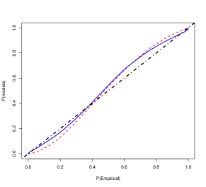
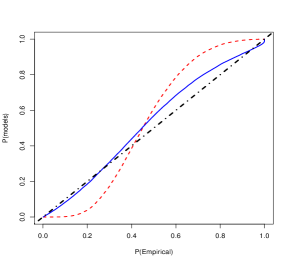
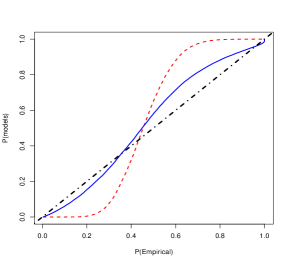
Figure 3: SAR(1) model: PP-plots for saddlepoint (continuous line) vs asymptotic normal (dotted line) probability approximation, for the MLE $\hat{\lambda}$, for $n=24$ and $n=100$, $\lambda_{0}=0.2$, and different $W_{n}$.

Saddlepoint vs Edgeworth expansion (testing simple hypotheses). The Edgeworth expansion derived in Proposition 3 represents the natural alternative to the saddlepoint approximation since it is fully analytic. To gain insights into the different behavior of the saddlepoint and Edgeworth approximations, we investigate the size of a hypothesis test based on the approximations. We set $n=24$ and we assume that $\sigma^{2}$ is known and equal to one. We consider the simple null hypothesis $H_{0}$: $\lambda_{0}=0$ for a one-sided test of zero against positive values of spatial correlation. We use 25,000 replications of $\hat{\lambda}_{n,T}$ to get the empirical estimate $\hat{F}_{0}$ of the c.d.f. $F_{0}$ of the estimator under the null hypothesis. We use the generic notation $G$ for the c.d.f. of one of the Edgeworth, or saddlepoint approximations, under the null hypothesis. For the sake of completeness, we also display the results for the Gaussian (first-order) approximation. The empirical rejection probabilities $\hat{\alpha}=1-\hat{F}_{0}(G^{-1}(1-\alpha))$ are shown in Figure 4 for nominal size $\alpha$ ranging from 1% to 10%, and correspond to an estimated size. We have overrejection when we are above the 45-degree line. We observe strong size distortions for the asymptotic and Edgeworth approximations as expected from the previous results. The saddlepoint approximation exhibits only mild size distortions. For example, we get an estimated size $\hat{\alpha}$ of 11.72%, 7.36%, 5.70%, for the Normal, Edgeworth, and saddlepoint approximations, for a nominal size of 5%.

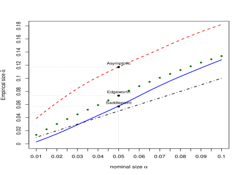
Figure 4: SAR(1) model: Estimated $\hat{\alpha}$ versus nominal size $\alpha$ between 1% and 10% under saddlepoint (continuous line), Edgeworth (dotted line with diamonds) and first-order asymptotic approximation (dotted line). $W_{n}$ is Rook, $n=24$ and $\lambda_{0}=0.0$.

Saddlepoint vs parametric bootstrap. The parametric bootstrap represents a (computer-based) competitor, commonly applied in statistics and econometrics. To compare our saddlepoint approximation to the one obtained by bootstrap, we consider different numbers of bootstrap repetitions, labeled as $B$: we use $B=499$ and $B=999$. For space constraints, in Figure 5, we display the results for $B=499$ (similar plots are available for $B=999$) showing the functional boxplots (as obtained iterating the procedure 100 times) of the bootstrap approximated density, for sample size $n=24$ and for $W_{n}$ is Queen.

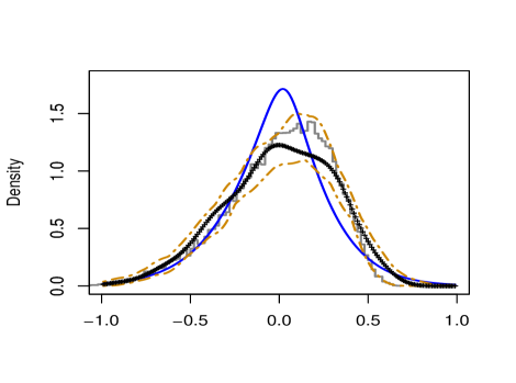
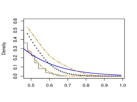
Figure 5: SAR(1) model. Left panel: Density plots for saddlepoint (continuous line) vs the functional boxplot of the parametric bootstrap probability approximation to the exact density (as expressed by the histogram and obtained using MC with size 25000), for the MLE $\hat{\lambda}$ and $W_{n}$ is Queen. Sample size is $n=24$, while $\lambda_{0}=0.2$. Right panel: zoom on the right tail. In each plot, we display the functional central curve (dotted line with crosses), the $1_{st}$ and $3_{rd}$ functional quartile (two-dash lines).

To visualize the variability entailed by the bootstrap, we display the first and third quartile curves (two-dash lines) and the median functional curve (dotted line with crosses); for details about functional boxplots, we refer to Sun and Genton, (2011) and to R routine fbplot. We notice that, while the bootstrap median functional curve (representing a typical bootstrap density approximation) is close to the actual density (as represented by the histogram), the range between the quartile curves illustrates that the bootstrap approximation has a variability. Clearly, the variability depends on $B$: the larger is $B$, the smaller is the variability. However, larger values of $B$ entail bigger computational costs: when $B=499$, the bootstrap is almost as fast as the saddlepoint density approximation (computation time about 7 minutes, on a 2.3 GHz Intel Core i5 processor), but for $B=999$, it is three times slower. We refer to Appendix D.5 for additional numerical results.

6.2 Testing in the presence of nuisance parameters

6.2.1 Saddlepoint test for composite hypotheses

Our saddlepoint density and/or tail approximations are helpful for testing simple hypotheses about $\theta_{0}$; see §6.1. Another interesting case suggested by the Associate Editor and an anonymous referee that has a strong practical relevance is related to testing a composite null hypothesis. It is a problem which is different from the one considered so far in the paper, because it raises the issue of dealing with nuisance parameters.

To tackle this problem, several possibilities are available. For instance, we may fix the nuisance parameters at the MLE estimates. Alternatively, we may consider to use the (re-centered) profile estimators, as suggested, e.g., in Hillier and Martellosio, (2018) and Martellosio and Hillier, (2020). Combined with the saddlepoint density in (4.13), these techniques yield a ready solution to the nuisance parameter problem. In our numerical experience (see Appendix D.6 for an experiment about the SAR(1)), these solutions may preserve reasonable accuracy in some cases. Nevertheless, the main theoretical drawback related to the use of MLE values for the nuisance parameter(s) is that it would not guarantee that the second-order properties derived in the previous sections still hold. To cope with this issue, we propose to build on Robinson et al., (2003), who derive a saddlepoint test statistic which takes into account explicitly the nuisance parameters, while preserving relative error in normal region. We feel this test statistic represents the natural candidate within our setting: it shares the same spirit as our saddlepoint density approximation and it is derived going through steps which are similar to ours. The paper by Robinson et al., (2003) defines the test statistic in the i.i.d. setting, while Lô and Ronchetti, (2009) and Czellar and Ronchetti, (2010) extend it to the non-i.i.d. data setting.

Let us consider a SARAR model whose parameter is $\theta=(\theta_{10},\theta_{2})^{\prime}$, where $\theta_{10}$ is specified by the null composite hypothesis: typically, the null concerns $\lambda$ only, while $\theta_{2}$ contains all the nuisance parameters. More specifically, the parameter is $\theta=(\lambda,\beta,\rho,\sigma^{2})^{\prime}$ and the general function $q(\theta)$ used in the previous sections is simply $q(\theta)=\lambda$. Thus, we have the composite hypothesis:

$$\mathcal{H}_{0}:\lambda=\lambda_{0}=0\quad\text{vs}\quad\mathcal{H}_{1}:\lambda>0,$$ (6.1)

where $\theta=(\lambda,\theta_{2})^{\prime}$, with $\theta_{10}=\lambda_{0}$ and $\theta_{2}=(\beta,\rho,\sigma^{2})^{\prime}$. Then, we define the test statistic

$${SAD}_{n}(\hat{\lambda})=2n\ \underset{\theta_{2}}{\inf}\ \underset{\nu}{\sup}\ -\mathcal{K}_{\psi}(\nu,\hat{\lambda},\theta_{2}).$$ (6.2)

The function $\mathcal{K}_{\psi}(\nu,(\lambda,\theta_{2}))$ is the c.g.f. of the estimating function:

$$\mathcal{K}_{\psi}(\nu,\hat{\lambda},\theta_{2})=n^{-1}\sum_{i=1}^{n}\ln E_{P_{(\lambda_{0},\theta_{2})}}\exp(\nu^{T}\psi_{i}^{(T)}(\hat{\lambda},\theta_{2})),$$ (6.3)

where $\psi_{i}^{(T)}(\lambda,\theta_{2}):=\sum_{t=1}^{T}(T-1)^{-1}\psi_{i,t}(\lambda,\theta_{2})$ and $\psi_{i,t}$ is as in (4.1). The c.g.f. $\mathcal{K}_{\psi}$ has a role analogous to the one of the c.g.f. of the $U$-statistic, that we derived in §4. We highlight that the expected value in (6.3) is taken w.r.t. the probability $P_{(\lambda_{0},\theta_{2})}$, where $\lambda_{0}$ is specified by the null, while the nuisance parameters are not fixed: the infimum over $\theta_{2}$ takes care of the nuisance parameters. In our inference procedure, we have that $\hat{\theta}_{n,T}=(\hat{\lambda},\hat{\theta}_{2})^{\prime}$ is the solution to $\sum_{i=1}^{n}\psi_{i}^{(T)}(\lambda,\theta_{2})=0.$ Under the null hypothesis, the test statistic ${SAD}_{n}(\hat{\lambda})$ is asymptotically $\chi_{1}^{2}$ distributed with a relative error of order $O(m^{-1})$ in the normal region.

6.2.2 Implementation aspects

To implement the test (6.2) for the problem (6.1), in Appendix C.2, we propose an algorithm (see Algorithm 2) and itemize the main steps needed to compute the test statistic.

6.2.3 Numerical results

Let us work with a SARAR(1,1) model, having no covariates and known variance $\sigma^{2}=1$ and $n=24$. It implies that $\theta=(\lambda,\rho)^{\prime}$ and we consider the problem in (6.1), with $\rho$ being the nuisance parameter. We set three different values $\rho=0.25,0.5,0.75$ to analyze numerically the impact that the spatial dependence in the innovation term has on $SAD_{n}$. We study the behaviour of the Wald test, as obtained using the first-order asymptotic theory and making use of the expression of the asymptotic variance as available in Appendix B. We compare the Wald test to $SAD_{n}$–to implement (6.2) we make use of the R routine nlm. We consider two types of spatial matrix $W_{n}$, the Rook and the Queen, and we set $W_{n}\equiv M_{n}$. Both test statistics are asymptotically $\chi_{1}^{2}$ distributed under the null hypothesis. To compare them in small samples, we first obtain the 95th and 97.5th quantile of each test statistic; then we compute the corresponding probability as obtained using the $\chi_{1}^{2}$. We display the results in Table 1. We see that the Wald test has severe size distortion. For instance, for $\rho=0.25$, we observe a relative error of about $30\%$, for the quantile of $95\%$, when $W_{n}$ is Rook, while the saddlepoint test entails a relative error of about $1.8\%$. Looking at the performance of ${SAD}_{n}$, we see that it is uniformly more accurate than the Wald test: considering all cases, we observe a maximal relative error of about $2\%$, for the quantile of $95\%$, when $\rho=0.75$ and $W_{n}$ is Queen; in the same setting, the Wald test entails a relative error of about $24\%$. Moreover, the size is fairly constant for the different values of $\rho$: it illustrates that the test statistic takes care correctly of the nuisance parameter.

		$\rho=0.25$				$\rho=0.5$				$\rho=0.75$
		$95.00\%$	$97.50\%$			$95.00\%$	$97.50\%$			$95.00\%$	$97.50\%$
Rook
	Wald	$66.08\%$	$89.89\%$			$98.33\%$	$99.41\%$			$99.99\%$	$99.99\%$
	${SAD}_{n}$	$96.71\%$	$97.18\%$			$96.66\%$	$97.18\%$			$95.55\%$	$96.04\%$
Queen
	Wald	$72.71\%$	$80.20\%$			$90.48\%$	$98.00\%$			$98.36\%$	$99.22\%$
	${SAD}_{n}$	$94.79\%$	$96.94\%$			$95.90\%$	$98.20\%$			$96.94\%$	$97.49\%$

Table 1: Wald and $SAD_{n}$ test for the problem (6.1)–spatial dependence in the presence of a nuisance parameter, in a SARAR(1,1) model–with no covariates and known variance. The quantiles are obtained using 100 repetitions of each test statistic.

7 Empirical application

Feldstein and Horioka, (1980) document empirically that domestic saving rate in a country has a positive correlation with the domestic investment rate. It contrasts with the understanding that, if capital is perfectly mobile between countries, most of any incremental saving is invested to get the highest return regardless of any locations, and that such correlation should actually vanish. Debarsy and Ertur, (2010) suggest to use spatial modeling since several papers challenge these findings but under the strong assumption that investment rates are independent across countries. Such an assumption might influence the conclusions of applied statial economics.

In this empirical exercise, we investigate the presence of spatial autocorrelation in the investment-saving relationship. We consider investment and saving rates for 24 OECD countries between 1960 and 2000 (41 years). Because of macroeconomic reasons (deregulating financial markets), we divide the whole period into shorter sub-periods: 1960-1970, 1971-1985 and 1986-2000, as advocated by Debarsy and Ertur, (2010). Since the cross-sectional size is only $n=24$, the asymptotics may suffer from size distortion as documented in §6. Therefore, we resort on a saddlepoint test to investigate whether or not there are inferential issues (coming from finite sample distortions and nuisance parameters) in the use of the first-order asymptotic theory. In line with the econometric literature, we specify the following SARAR(1,1) model for the three sub-periods:

$$\text{ Inv}_{nt} =\lambda_{0}W_{n}\text{ Inv}_{nt}+\beta_{0}\text{Sav}_{nt}+c_{n0}+E_{nt},$$ (7.1)

$$E_{nt} =\rho_{0}M_{n}E_{nt}+V_{nt}, \quad t=1,2,\cdots,T$$

where $\text{Inv}_{nt}$ is the $n\times 1$ vector of investment rates for all countries and $\text{Sav}_{nt}$ is the $n\times 1$ vector of saving rates. Each element $v_{it}$ in $V_{nt}$ is i.i.d across $i$ and $t$, having Gaussian distribution with zero mean and variance $\sigma_{0}^{2}$. $c_{n0}$ is the vector of fixed effects.

We assume $W_{n}=M_{n}$ and adopt two different weight matrices as in Debarsy and Ertur, (2010). The first one is based on the inverse distance. Each element $\omega_{ij}$ in $W_{n}$ is $d_{ij}^{-1}$, where $d_{ij}$ is the arc distance between capitals of countries $i$ and $j$. The second is the binary seven nearest neighbors (7NN) weight matrix. More precisely, $\omega_{ij}$=1, if $d_{ij}\leq d_{i}$ and $i\neq j$. Otherwise, $\omega_{ij}=0$, where $d_{i}$ is the $7_{th}$ order smallest arc-distance between countries $i$ and $j$ such that each country $i$ has exactly 7 neighbors. Both weight matrices are row-normalized.

We estimate the parameters using the MLE described in §3. Table 2 gathers the point estimates (and their standard errors) that agree with the magnitudes found by Debarsy and Ertur, (2010). To investigate the validity of the model (7.1), we test for spatial dependence, working on $\lambda=0$ and/or $\rho=0$. Specifically, our aim is to detect if and in which period(s) the inference yielded by the first-order asymptotic theory differs from the inference obtained using our saddlepoint test. With this goal, in Table 3 we provide the $p$-values for testing (at the $5\%$ level) three different composite hypotheses: in the first row, we consider the problem of testing for $\lambda=0$; in the second row, we test for $\rho=0$; in the third row, we test for $\lambda=\rho=0$. To perform the tests, we consider the routinely-applied Wald test (as obtained using the first-order asymptotic approximation, ASY) and the saddlepoint test ($SAD_{n}$). In each testing procedure, we treat the parameters not specified by the null hypothesis as nuisance parameters. In the $SAD_{n}$ test, we take care of the nuisance as indicated in (6.2), while in the ASY test we simply plug-in the MLE estimates for the nuisance parameters—as it is customary in the econometric software based on the first-order asymptotic theory.

In the period 60-70, both ASY and $SAD_{n}$ yield the same inference, for both the considered types of weight matrix, with conventional significance levels. The other sub-periods display some discrepancies between the inference obtained via ASY and via $SAD_{n}$. We do not want to discuss all discrepancies but only briefly comment on some key differences—we highlights the corresponding values in Table 3. In the sub-period 71-85 under 7NN $W_{n}$, the saddlepoint test finds no evidence against no spatial dependence in the investing rates across countries, and vice-versa for the asymptotic approximation. Moreover, the ASY test does not find evidence against $\rho=0$, while the $SAD_{n}$ test rejects this composite hypothesis. Thus, the $SAD_{n}$ test indicates a spillover through the contemporary shocks between countries. This spillover goes through the innovations, i.e., through the unexpected part of the model dynamics, a finding not documentable when one relies on the first-order asymptotic theory. This results suggests that a test statistic designed to perform well in small samples and in the presence of nuisance parameters is able to document spatial dependence in the disturbances $E_{nt}$. Some differences are detectable also in the sub-period 86-00, under the inverse distance matrix.

	Weight matrix: inverse distance				Weight matrix: 7 nearest neighbours
	1960-1970	1971-1985	1986-2000		1960-1970	1971-1985	1986-2000
$\beta$	0.935(0.05)	0.638(0.04)	0.356(0.07)		0.932(0.05)	0.633(0.04)	0.368(0.07)
$\lambda$	0.004(0.10)	0.381(0.11)	0.430(0.30)		-0.016(0.09)	0.340(0.10)	0.437(0.18)
$\rho$	-0.305(0.22)	0.334(0.16)	0.222(0.40)		-0.219(0.19)	0.258(0.15)	0.025(0.28)

Table 2: SARAR(1,1) model: Maximum likelihood estimates of Parameters $\beta$, $\lambda$, $\rho$. Standard errors are between brackets.

		Weight matrix: inverse distance				Weight matrix: 7 nearest neighbours
		1960-1970	1971-1985	1986-2000		1960-1970	1971-1985	1986-2000
$\lambda=0$	$SAD_{n}$	1.0000	0.0096	0.0000		0.9998	0.2248	0.0000
	ASY	1.0000	0.0116	0.5679		0.9987	0.0130	0.1123
$\rho=0$	$SAD_{n}$	0.1134	0.0024	0.1217		0.3232	0.0403	0.9993
	ASY	0.5890	0.2261	0.9578		0.7101	0.3898	0.9998
$\lambda=\rho=0$	$SAD_{n}$	0.1414	0.0000	0.0000		0.2603	0.0000	0.0000
	ASY	0.4615	0.0000	0.0000		0.5042	0.0000	0.0000

Table 3: SARAR(1,1) model: $p$-values of Saddlepoint ($SAD_{n}$) and Wald (ASY) tests for several composite hypotheses.

SUPPLEMENTARY MATERIAL

The online supplementary material includes proofs, lengthy analytical derivations and additional numerical results for the SAR(1) model. All the codes and data are available in our Github repository.

References

- Anselin, (1988) Anselin, L. (1988), Spatial Econometrics: Methods and Models, vl. 4, Springer, New York.
- Baltagi, (2008) Baltagi, B. (2008), Econometric Analysis of Panel Data, vl. 1, Wiley, New York.
- Bao, (2013) Bao, Y. (2013), Finite-sample Bias of the QMLE in Spatial Autoregressive Models, Econometric Theory, 29, 68–89.
- Bao and Ullah, (2007) Bao, Y. and Ullah, A. (2007), Finite Sample Properties of Maximum Likelihood Estimator in Spatial Models, Journal of Econometrics, 137, 396–413.
- Barndorff-Nielsen and Cox, (1989) Barndorff-Nielsen, O. and Cox, D. (1989), Asymptotic Techniques for Use in Statistics, Chapman and Hall, London.
- Bickel et al., (1986) Bickel, P., Götze, F., and Van Zwet, W. (1986), The Edgeworth Expansion for U-statistics of Degree Two, The Annals of Statistics, 14, 1463–1484.
- Brazzale et al., (2007) Brazzale, A., Davison, A. C., and Reid, N. (2007), Applied Asymptotics: Case Studies in Small-Sample Statistics, vl. 23, Cambridge University Press.
- Cressie, (2015) Cressie, N. (2015), Statistics for Spatial Data, Wiley, New York.
- Cressie and Wikle, (2015) Cressie, N. and Wikle, C. (2015), Statistics for Spatio-Temporal Data, Wiley, New York.
- Czellar and Ronchetti, (2010) Czellar, V. and Ronchetti, E. (2010), Accurate and Robust Tests for Indirect Inference, Biometrika, 97, 621–630.
- Daniels, (1954) Daniels, H. E. (1954), Saddlepoint Approximations in Statistics, Annals of Mathematical Statistics, 25, 631–650.
- Debarsy and Ertur, (2010) Debarsy, N. and Ertur, C. (2010), Testing for Spatial Autocorrelation in a Fixed Effects Panel Data Model, Regional Science and Urban Economics, 40, 453–470.
- Durbin, (1980) Durbin, J. (1980), Approximations for Densities of Sufficient Estimators, Biometrika, 67, 311–333.
- Easton and Ronchetti, (1986) Easton, G. S. and Ronchetti, E. (1986), General Saddlepoint Approximations With Applications to L-statistics, Journal of the American Statistical Association, 81, 420–430.