Stochastic homogenization on randomly perforated domains
Abstract
We study the existence of uniformly bounded extension and trace operators for -functions on randomly perforated domains, where the geometry is assumed to be stationary ergodic. Such extension and trace operators are important for compactness in stochastic homogenization. In contrast to former approaches and results, we use very weak assumptions on the geometry which we call local -regularity, isotropic cone mixing and bounded average connectivity. The first concept measures local Lipschitz regularity of the domain while the second measures the mesoscopic distribution of void space. The third is the most tricky part and measures the "mesoscopic" connectivity of the geometry.
In contrast to former approaches we do not require a minimal distance between the inclusions and we allow for globally unbounded Lipschitz constants and percolating holes. We will illustrate our method by applying it to the Boolean model based on a Poisson point process and to a Delaunay pipe process.
We finally introduce suitable Sobolev spaces on and in order to construct a stochastic two-scale convergence method and apply the resulting theory to the homogenization of a -Laplace problem on a randomly perforated domain.
1 Introduction
In 1979 Papanicolaou and Varadhan [31] and Kozlov [24] for the first time independently introduced concepts for the averaging of random elliptic operators. At that time, the periodic homogenization theory had already advanced to some extend (as can be seen in the book [32] that had appeared one year before) dealing also with non-uniformly elliptic operators [26] and domains with periodic holes [7].
Even though the works [24, 31] clearly guide the way to a stochastic homogenization theory, this theory advanced quite slowly over the past 4 decades. Compared to the stochastic case, periodic homogenization developed very strong with methods that are now well developed and broadly used. The most popular methods today seem to be the two-scale convergence method by Allaire and Nguetseng [2, 30] in 1989/1992 and the periodic unfolding method [6] by Cioranescu, Damlamian and Griso in 2002. Both methods are conceptually related to asymptotic expansion and very intuitive to handle. It is interesting to observe that the stochastic counterpart, the stochastic two-scale convergence, was developed only in 2006 by Zhikov and Piatnitsky [39], with the stochastic unfolding developed only recently in [29, 19].
A further work by Bourgeat, Mikelic and Wright [5] introduced two-scale convergence in the mean. This sense of two-scale convergence is indeed a special case of the stochastic unfolding, which can only be applied in an averaged sense, too. This leads us to a fundamental difference between the periodic and the stochastic homogenization. In stochastic homogenization we distinguish between quenched convergence, i.e. for almost every realization one can prove homogenization, and homogenization in the mean, which means that homogenization takes place in expectation.
In particular in nonlinear non-convex problems (that is: we cannot rely on weak convergence methods) the quenched convergence is of uttermost importance, as this sense of convergence allows to use - for each fixed - compactness in the spaces . On the other hand, convergence in the mean deals with convergence in , which goes in hand with a loss of compactness.
The results presented below are meant for application in quenched convergence. The estimates for the extension and trace operators which are derived strongly depends on the realization of the geometry - thus on . Nevertheless, if the geometry is stationary, a corresponding estimate can be achieved for almost every .
The Problem
The discrepancy in the speed of progress between periodic and stochastic homogenization is due to technical problems that arise from the randomness of parameters. In this work we will consider uniform extension operators for randomly perforated stationary domains. We use stationarity (see Def. 2.16) as this is the standard way to cope with the lack of periodicity. Let us first have a look at a typical application to illustrate the need of the extension operators that we construct below.
Let be a stationary random open set and let be the smallness parameter and let be a connected component of . For a bounded open domain, we consider and with outer normal . We study the following problem in Section 10.6:
| (1.1) | |||||
Note that for simplicity of illustration, the only randomness that we consider in this problem is due to , i.e. we assume .
Problem (1.1) can be recast into a variational problem, i.e. solutions of (1.1) are local minimizers of the energy functional
where is convex with . This problem will be treated in Theorem 10.20 and the final Remark 10.22.
One way to prove homogenization of (1.1) is to prove -convergence of . Conceptually, this implies convergence of the minimizers to a minimizer of the limit functional. However, the minimizers are elements of and since this space changes with , we lack compactness in order to pass to the limit in the nonlinearity. The canonical path to circumvent this issue in periodic homogenization is via uniformly bounded extension operators , see [20, 22], combined with uniformly bounded trace operators, see [12, 13].
The first proof for the existence of periodic extension operators was due to Cioranescu and Paulin [7] in 1979, while the proof in its full generality was provided only recently by Höpker and Böhm [22] and Hp̈ker [21]. In this work we will generalize parts of the results of [21] to a stochastic setting. A modified version of the original proof of [21] is provided in Section 3. It relies on three ingredients: the local Lipschitz regularity of the surface, the periodicity of the geometry and the connectedness. Local Lipschitz regularity together with periodicity imply global Lipschitz regularity of the surface. In particular, one can construct a local extension operator on every cell , which might then be glued together using a periodic partition of unity of . The connectedness of the geometry assures that the difference of the average of a function on two different cells and can be computed from the gradient along a path connecting the two cells and being fully comprised in .
In the stochastic case the proof of existence of suitable extension operators is much more involved and not every geometry will eventually allow us to be successful. In fact, we will not be able - in general - to even provide extension operators but rather obtain , where depends (among others) on the dimension and on the distribution of the Lipschitz constant of . This is due to the presence of arbitrarily “bad” local behavior of the geometry.
The theory developed below also allows to provide estimates on the trace operator
when seen as an operator , where again in general.
We summarize the above discussion in the following.
Problem 1.1.
Find (computationally or rigorously) verifiable conditions on stationary random geometries that allow to prove existence of extension operators
where and are independent of and where
Problem 1.2.
Find (computationally or rigorously) verifiable conditions on stationary random geometries that allow to prove an estimate
where and are independent of .
Let us mention at this place existing results in literature. In recent years, Guillen and Kim [13] have proved existence of uniformly bounded extension operators in the context of minimally smooth surfaces, i.e. uniformly Lipschitz and uniformly bounded inclusions with uniform minimal distance. A homogenization result of integral functionals on randomly perforated domains with uniformly bounded inclusions was provided by Piat and Piatnitsky [33]. Concerning unbounded inclusions and non-uniformly Lipschitz geometries, the present work seems to be the first approach. Since Problem 1.2 is easier to handle, we first explain our concept of microscopic regularity in view of and then go on to extension operators.
-Regularity and the Trace Operator
We introduce two concepts which are suited for the current and potentially also for further studies. The first of these two concepts is inspired by the concept of minimal smoothness [35] and accounts for the local regularity of . Deviating from [35] we will call it local -regularity (see Definition 4.2). Although this assumption is very weak, its consequences concerning local coverings of are powerful. Based on this concept, we introduce the functions , and on as well as and for in Lemmas 4.4, 4.6, 4.8 and 4.12 and make the following assumptions:
Assumption 1.3.
Let be a random open set such that for and it holds either
Having studied the properties of -regular sets in detail in Sections 4.1 and 2.5 it is very easy to prove the following trace theorem (for notations we refer to Section 2 and Section 4.1). Note that via a simple rescaling, this provides a solution to Problem 1.1.
Theorem 1.4 (Solution of Problem 1.1).
Let be a stationary and ergodic random open set which is almost surely locally regular and let Assumption 1.3 hold. For given let be the trace operator. Then for almost every the extension is continuous and there exists a constant s.t. it holds for every bounded Lipschitz domain and every
Proof.
This is a consequence of Theorem 5.9, stationarity and ergodicity and the ergodic theorem. ∎
Construction of Extension Operators
The main results of this work is on extension operators on randomly perforated domains. In order to construct a suitable extension operator, we use
Step 1: -regularity
Concerning extension results, the concept of -regularity suggests the naive approach to use a local open covering of and to add the local extension operators via a partition of unity in order to construct a global extension operator. We call this ansatz naive since one would not chose this approach even in the periodic setting, as it is known to lead to unbounded gradients. Nevertheless, this ansatz is followed in Section 5.2 for two reasons. The first reason is illustration of an important principle: The extension operator can be split up into a local part , whose norm can be estimated by local properties of , and a global part whose norm is determined by connectivity, an issue which has to be resolved afterwards, and corresponds to Step 2 in the proof of Theorem 3.2 below (periodic case), where one glues together the local extension operators on the periodic cells. The second reason is that this first estimate, although it cannot be applied globally, is very well suited for constructing a local extension operator. Lemma 5.6 hence provides estimates of a certain extension operator which has the property that the constant in the estimate tends to as the domain grows.
However, this first ansatz grants some insight into the structure of the extension problem. In particular, we find the following result which will provide a better understanding of the Sobolev spaces and on the probability space .
Assumption 1.5.
Theorem 1.6.
Theorem 1.6, though useful, is not satisfactory for homogenization, as is bounded by and not solely . Therefore, some more work is needed.
Step 2: isotropic cone mixing
In order to account for the issue of connectedness in a proper way on the macroscopic level, we propose our second fundamental concept of isotropic cone mixing geometries (see Definition 4.17), which allow to construct a global Voronoi tessellation of with good local covering properties. This definition, though being rather technical, can be verified rather easily using Criterion 4.18.
In short, isotropic cone mixing allows to distribute balls of a uniform minimal radius within such that the centers of the balls generate a Voronoi mesh of cells with diameter , distributed according to a function (see Lemma 4.20). These Voronoi cells in general might be of arbitrary large diameter , although they are bounded in the statistical average. Due to this lack of a uniform bound, we call the distribution of Voronoi cells the mesoscopic regularity of the geometry.
Step 3: gluing
The Voronoi cells resulting from an isotropic cone mixing geometry are well suited for the gluing of local extension operators. We will construct the macroscopic extension operator in an analogue way to [21], replacing the periodic cells by the Voronoi cells (see Figure 5). In Theorem 6.3 we provide a first abstract result how the norm of the glued operator can be estimated from the distribution of , the geometry of the Voronoi mesh and the connectivity, even though the last two properties enter rather indirectly. To make this more clear, we note at this points that the extension operator depends on two types of local averages: To each Voronoi cell we take the average over . Furthermore, to every local microscopic extension operator chosen in Section 5 there corresponds a local average close to the boundary. We will see that the norm of the extension operator strongly depends on the differences and .
In Theorem 6.7 we will see that the dependence on can be eliminated with the price to increase the cost of “unfortunate distributions” of and of the local regularity. The remaining dependence which we leave unresolved is the dependence on . This dependence is linked to quantitative connectedness properties of the geometry. By this we mean more than the topological question of connectedness. In particular, we need an estimate of the type which will finally allow us an estimate of in terms of . Unfortunately, the classical percolation theory, which deals with connectedness of random geometries, is not developed to answer this question. In this paper, we will use two workarounds which we call “statistically harmonic” and “statistically connected”. However, further research has to be conducted. We state our first main theorem.
Theorem 1.7.
Let be a stationary ergodic random open set which is almost surely -regular (Def. 4.2) and isotropic cone mixing for and (Def. 4.17) and statistically harmonic (Def. 6.9) and let . Let be bounded open with Lipschitz boundary as well as such that
Then for almost every the extension operator provided in (6.6) is well defined with a constant such that for every positive
Proof.
In practical applications, one would need to verify whether is statistically harmonic via numerical simulations. The problem particularly results in the numerical evaluation of a Laplace operator.
Based on this insight, we develop an alternative approach: The connectedness of is quantified by introducing directly a discrete graph on and a discrete Poisson equation on this graph. The construction of the graph and the evaluation of the Poisson equation can be done numerically, but with the advantage that the discrete quantities are now directly connected to the analytical theory. Additionally to the -regularity we have to deal with the average diameter of the cells of a the global Voronoi tessellation and the local stretch factor . We impose the following assumptions:
Assumption 1.8.
Let be a random open set such that Assumption 5.5 hold and let be the constant from (5.8). Let (1.2) and for let either
or
Furthermore, let be almost surely isotropic cone mixing for and (Def. 4.17) as well as locally connected and let the local stretch factor (see Definition Theorem 7.7 and Definition 7.8) satisfy such that
The second main theorem can be formulated as follows:
Theorem 1.9.
Let be a stationary ergodic random open set which is almost surely -regular (Def. 4.2) and isotropic cone mixing for and (Def. 4.17) as well as locally connected and satisfy such that Assumption 1.8 holds. For and a bounded domain with Lipschitz boundary. Then for almost every the extension operator provided in (6.6) is well defined with a constant such that for every positive and every
| (1.3) | ||||
| (1.4) |
Sobolev Spaces on
Besides the evident benefit of the above extension and trace theorems, let us note that these theorems are also needed for the construction of the suitable Sobolev spaces on . In Section 9 we recall some standard construction of Sobolev spaces on the probability space and provide some links between two major approaches which seem to be hard to find in one place. We will need this summing up in order to better illustrate the generalization to perforated domains.
To understand our ansatz, we recall a result from [14] that there exist and such that for almost every and , where . The random set leads to Sobolev spaces , e.g. by defining . We will see that we can introduce spaces , but this construction is more involved than in and heavily relies on the almost sure extension property guarantied by Theorem 1.6. Once we have introduced the spaces we can also introduce “trace”-operators , where with , and is to be understood w.r.t. the Palm measure on . This construction will rely on Theorems 1.6 and 1.4. In all our results, we only provide sufficient conditions for the existence of the respective spaces and operators. Necessary conditions are left for future studies.
Discussion: Random Geometries and Applicability of the Method
In Section 10 we will discuss how the present results can be applied in the framework of the stochastic two-scale convergence method. However, this concerns only the analytic aspect of applicability.
The more important question is the applicability of the presented theory from the point of view of random geometries. Of course our result can be applied to periodic geometries and hence also to stochastic geometries which originate from random perturbations of periodic geometries as long as these perturbations are - in the statistical average - “not to large”. However, it is a well justified question if the estimates presented here are applicable also for other models.
In Section 8 we discuss three standard models from the theory of stochastic geometries. The first one is the Boolean model based on a Poisson point process. Here we can show that the micro- and mesoscopic assumptions are fulfilled, at least in case is given as the union of balls. If we choose as the complement of the balls, we currently seem to run into difficulties. However, this problem might be overcome using a Matern modification of the Poisson process. We deal with such Matern modifications in Section 8.2. What remains challenging in both settings are the proofs of statistical harmony or statistical connectivity. However, if the Matern process strongly excludes points that are to close to each other, the connectivity issue can be resolved.
A further class which will be discussed are a system of Delaunay pipes based on a Matern process. In this case, even though the geometry might locally become very irregular, all properties can be verified. Hence, we identified at least one non-trivial, non-quasi-periodic geometry to which our approach can be applied for sure.
The above mentioned construction of Sobolev spaces and the application in the homogenization result of Theorem 10.20 clearly demonstrate the benefits of the new methodology.
Notes
Structure of the article
We close the introduction by providing an overview over the article and its main contributions. In Section 2 we collect some basic concepts and inequalities from the theory of Sobolev spaces, random geometries and discrete and continuous ergodic theory. We furthermore establish local regularity properties for what we call -regular sets, as well as a related covering theorem in Section 2.5. In Section 2.11 we will demonstrate that stationary ergodic random open sets induce stationary processes on , a fact which is used later in the construction of the mesoscopic Voronoi tessellation in Section 4.2.
In Section 3 we provide a proof of the periodic extension result in a simplified setting. This is for completeness and self-containedness of the paper, in order to make a comparison between stochastic and periodic approach easily accessible to the reader.
In Section 4 we introduce the regularity concepts of this work. More precisely, in Section 4.1 we introduce the concept of local -regularity and use the theory of Section 2.5 in order to establish a local covering result for , which will allow us to infer most of our extension and trace results. In Section 4.2 we show how isotropic cone mixing geometries allow us to construct a stationary Voronoi tessellation of such that all related quantities like “diameter” of the cells are stationary variables whose expectation can be expressed in terms of the isotropic cone mixing function . Moreover we prove the important integration Lemma 4.21.
A Remark on Notation
This article uses concepts from partial differential equations, measure theory, probability theory and random geometry. Additionally, we introduce concepts which we believe have not been introduced before. This makes it difficult to introduce readable self contained notation (the most important aspect being symbols used with different meaning) and enforces the use of various different mathematical fonts. Therefore, we provide an index of notation at the end of this work. As a rough orientation, the reader may keep the following in mind:
We use the standard notation , , , for natural (), rational, real and integer numbers. denotes a probability measure, the expectation. Furthermore, we use special notation for some geometrical objects, i.e. for the torus ( equipped with the topology of the torus), the open interval as a subset of (we often omit the index ), a ball, a cone and a set of points. In the context of finite sets , we write for the number of elements.
Bold large symbols (, , ,) refer to open subsets of or to closed subsets with . The Greek letter refers to a dimensional manifold (aside from the notion of -convergence).
Calligraphic symbols (, , ) usually refer to operators and large Gothic symbols () indicate topological spaces, except for .
2 Preliminaries
We first collect some notation and mathematical concepts which will be frequently used throughout this paper. We first start with the standard geometric objects, which will be labeled by bold letters.
2.1 Fundamental Geometric Objects
Unit cube The torus has the topology of the metric . In contrast, the open interval is considered as a subset of . We often omit the index if this does not provoke confusion.
Balls Given a metric space we denote the open ball around with radius . The surface of the unit ball in is .
Points A sequence of points will be labeled by .
A cone in is usually labeled by . In particular, we define for a vector of unit length, and the cone
Inner and outer hull We use balls of radius to define for a closed set the sets
| (2.1) | ||||
One can consider these sets as inner and outer hulls of . The last definition resembles a concept of “negative distance” of to and “positive distance” of to . For we denote the closed convex hull of .
The natural geometric measures we use in this work are the Lebesgue measure on , written for , and the -dimensional Hausdorff measure, denoted by on -dimensional submanifolds of (for ).
2.2 Local Extensions and Traces
Let be an open set and let and be a constant such that is graph of a Lipschitz function. We denote
| (2.2) |
Remark 2.1.
For every , the function is monotone increasing in .
In the following, we formulate some extension and trace results. Although it is well known how such results are proved and the proofs are standard, we include them for completeness.
Lemma 2.2 (Uniform Extension for Balls).
Let be an open set, and assume there exists , and an open domain such that is graph of a Lipschitz function of the form in with Lipschitz constant and . Writing and defining there exist an extension operator
| (2.3) |
such that for
| (2.4) |
and for every the operator
is continuous with
| (2.5) |
Remark 2.3.
It is well known ([10, chapter 5]) that for every bounded domain with -boundary there exists a continuous extension operator .
Proof of Lemma 2.2.
The extended function , is bijective with . In particular, both and are Lipschitz continuous with Lipschitz constant .
W.l.o.g. we assume that
implying .
Step 1: We consider the extension operator having the form [10, chapter 5], [1]
We make use of this operator and define
Note that all three operators , and map -functions to -functions. By the definition of we may explicitly calculate (2.3). In particular, is well defined for whenever
| (2.6) |
Step 2: We seek for such that (2.6) is satisfied for every and such that . For and , we find with and that
In particular,
and (2.6) holds if
Hence we require . It is now easy to verify (2.5) from the definition of and the chain rule. ∎
Lemma 2.4.
Let be an open set, and assume there exists , and an open domain such that is graph of a Lipschitz function of the form in with Lipschitz constant and . Writing we consider the trace operator . For every and every the operator can be continuously extended to
such that
| (2.7) |
2.3 Poincaré Inequalities
We denote
Note that this is not a linear vector space.
Lemma 2.5.
For every there exists such that the following holds: Let and such that then for every
| (2.8) |
and for every it holds
| (2.9) |
Remark.
In case we find that (2.9) holds iff for some .
Proof.
In a first step, we assume . The underlying idea of the proof is to compare every , with . In particular, we obtain for that
and hence by Jensen’s inequality
We integrate the last expression over and find
For general , use the extension operator (see Remark 2.3) such that and . Since we infer
and hence (2.8). Furthermore, since there
holds
for every , a scaling argument shows
for every
and hence (2.9).
∎
Lemma 2.6.
Let and and (if ) or (if ). Then there exists such that for every convex set with polytope boundary
| (2.10) |
and for every
| (2.11) |
where
| (2.12) |
Remark 2.7.
For the critical Sobolev index we infer .
Proof.
First note that by a simple scaling argument based on the integral transformation rule the equations (2.8) yields for every
| (2.13) |
and (2.9) yields for every
| (2.14) |
Now, for we denote as the unique and for we denote and consider the bijective Lipschitz map
Then we infer from (2.13)
or, after transformation of integrals,
It remains to estimate the derivatives of . In polar coordinates, the radial derivative is , while the tangential derivative is more complicated to calculate. However, in case we obtain , which is by the same time the minimal absolute value for each tangential derivative, and becomes maximal in edges where and (see Figure …… ).Now we make use of the fact that increases the volume locally with a rate smaller than and hence . On the other hand, we have and hence (2.10). In a similar way we infer (2.11) from (2.14). ∎
2.4 Voronoi Tessellations and Delaunay Triangulation
Definition 2.8 (Voronoi Tessellation).
Let be a sequence of points in with if . For each let
Then is called the Voronoi tessellation of w.r.t. . For each we define .
We will need the following result on Voronoi tessellation of a minimal diameter.
Lemma 2.9.
Let and let be a sequence of points in with if . For let . Then
| (2.15) |
Proof.
Let the neighbors of and . Then all satisfy . Moreover, every with has the property that and . Since every Voronoi cell contains a ball of radius , this implies that . ∎
Definition 2.10 (Delaunay Triangulation).
Let be a sequence of points in with if . The Delaunay triangulation is the dual graph of the Voronoi tessellation, i.e. we say .
2.5 Local -Regularity
We say that a function holds “true” in if and “false” if .
Definition 2.11 (-regularity).
A set is called locally -regular with and if is decreasing and
| (2.16) |
For we write .
Lemma 2.12.
Let be a locally -regular set with and and . Then is locally Lipschitz continuous with Lipschitz constant and for every and it holds
| (2.17) |
Furthermore,
| (2.18) |
Proof.
We infer from (2.16) for every and such that let such that also . It then holds and hence . Taking the supremum over we find i.e.
which implies . This in turn leads to or
implying (2.17) and continuity of .
Let , the last inequality particularly implies also . Together with we have
Finally, in order to prove (2.18), w.l.o.g. let . Then
∎
We make use of the latter Lemmas in order to prove the following covering-regularity of .
Theorem 2.13.
Let be a closed set and let be bounded and satisfy for every and for
| (2.19) |
and define , . Then for every there exists a locally finite covering of with balls for a countable number of points such that for every with it holds
| (2.20) | ||||
| and |
Proof.
W.o.l.g. assume . Consider , let denote the elements of and let . We set , , and for we construct the covering using inductively defined open sets and closed set as follows:
-
1.
Define . For do the following:
-
(a)
For every do
then set otherwise set -
(b)
Define and and .
Observe: implies and , implies and hence . Similar, , , implies .
-
(a)
-
2.
Define , .
The above covering of is complete in the sense that every lies into one of the balls (by contradiction). We denote the family of centers of the above constructed covering of and find the following properties: Let be such that . W.l.o.g. let . Then the following two properties are satisfied due to (2.19)
-
1.
It holds and hence and . Furthermore .
-
2.
Let such that . If also then observation 1.(b) implies . If then and hence , implying .
Choosing and appropriately, this concludes the proof. ∎
2.6 Dynamical Systems
Assumption 2.14.
Throughout this work we assume that is a probability space with countably generated -algebra .
Due to the insight in [14], shortly sketched in the next two subsections, after a measurable transformation the probability space can be assumed to be metric and separable, which always ensures Assumption 2.14.
Definition 2.15 (Dynamical system).
A dynamical system on is a family of measurable bijective mappings satisfying (i)-(iii):
-
(i)
, (Group property)
-
(ii)
(Measure preserving)
-
(iii)
is measurable (Measurability of evaluation)
A set is almost invariant if . The family
| (2.21) |
of almost invariant sets is -algebra and
| (2.22) |
A concept linked to dynamical systems is the concept of stationarity.
Definition 2.16 (Stationary).
Let be a measurable space and let . Then is called (weakly) stationary if for (almost) every .
Definition 2.17.
A family is called convex averaging sequence if
-
(i)
each is convex
-
(ii)
for every holds
-
(iii)
there exists a sequence with as such that .
We sometimes may take the following stronger assumption.
Definition 2.18.
A convex averaging sequence is called regular if
The latter condition is evidently fulfilled for sequences of cones or balls. Convex averaging sequences are important in the context of ergodic theorems.
Theorem 2.19 (Ergodic Theorem [8] Theorems 10.2.II and also [36]).
Let be a convex averaging sequence, let be a dynamical system on with invariant -algebra and let be measurable with . Then for almost all
| (2.23) |
We observe that is of particular importance. For the calculations in this work, we will particularly focus on the case of trivial . This is called ergodicity, as we will explain in the following.
Definition 2.20 (Ergodicity and Mixing).
A dynamical system which is given on a probability space is called mixing if for every measurable it holds
| (2.24) |
A dynamical system is called ergodic if
| (2.25) |
Remark 2.21.
a) Let with the trivial -algebra and . Then is evidently mixing. However, the realizations are constant functions on for some constant .
b) A typical ergodic system is given by with the Lebesgue -algebra and the Lebesgue measure. The dynamical system is given by .
c) It is known that is ergodic if and only if every almost invariant set has probability (see [8] Proposition 10.3.III) i.e.
| (2.26) |
A further useful property of ergodic dynamical systems, which we will use below, is the following:
Lemma 2.22 (Ergodic times mixing is ergodic).
Let and be probability spaces with dynamical systems and respectively. Let be the usual product measure space with the notation for and . If is ergodic and is mixing, then is ergodic.
Proof.
Remark 2.23.
The above proof heavily relies on the mixing property of . Note that for being only ergodic, the statement is wrong, as can be seen from the product of two periodic processes in (see Remark 2.21). Here, the invariant sets are given by for arbitrary measurable .
2.7 Random Measures and Palm Theory
We recall some facts from random measure theory (see [8]) which will be needed for homogenization. Let denote the space of locally bounded Borel measures on (i.e. bounded on every bounded Borel-measurable set) equipped with the Vague topology, which is generated by the sets
This topology is metrizable, complete and countably generated. However, note that it is not locally compact, which implies that the Alexandroff compactification cannot be applied. A random measure is a measurable mapping
which is equivalent to both of the following conditions
-
1.
For every bounded Borel set the map is measurable
-
2.
For every the map is measurable.
A random measure is stationary if the distribution of is invariant under translations of that is and share the same distribution. From stationarity of one concludes the existence ([14, 31] and references therein) of a dynamical system on such that . By a deep theorem due to Mecke (see [28, 8]) the measure
can be defined on for every positive with compact support. is independent from and in case we find . Furthermore, for every -measurable non negative or - integrable functions the Campbell formula
holds. The measure has finite intensity if .
Theorem 2.24 (Ergodic Theorem [8] 12.2.VIII).
Let be a probability space, be a convex averaging sequence, let be a dynamical system on with invariant -algebra and let be measurable with . Then for -almost all
| (2.30) |
Given a bounded open (and convex) set , it is not hard to see that the following generalization holds:
Theorem 2.25 (General Ergodic Theorem).
Let be a probability space, be a convex bounded open set with , let be a dynamical system on with invariant -algebra and let be measurable with . Then for -almost all it holds
| (2.31) |
Sketch of proof.
Chose a countable family of characteristic functions that spans . Use a Cantor argument and Theorem 2.24 to prove the statement for a countable dense family of . From here, we conclude by density.
The last result can be used to prove the most general ergodic theorem which we will use in this work: ∎
Theorem 2.26 (General Ergodic Theorem for the Lebesgue measure).
Let be a probability space, be a convex bounded open set with , let be a dynamical system on with invariant -algebra and let and , where , . Then for -almost all it holds
Proof.
Let with . Then
which implies the claim. ∎
2.8 Random Sets
The theory of random measures and the theory of random geometry are closely related. In what follows, we recapitulate those results that are important in the context of the theory developed below and shed some light on the correlations between random sets and random measures.
Let denote the set of all closed sets in . We write
| (2.32) | |||||
| (2.33) |
The Fell-topology is created by all sets and and the topological space is compact, Hausdorff and separable[27].
Remark 2.27.
We find for closed sets in that if and only if [27]
-
1.
for every there exists such that and
-
2.
if is a subsequence, then every convergent sequence with satisfies .
If we restrict the Fell-topology to the compact sets it is equivalent with the Hausdorff topology given by the Hausdorff distance
Remark 2.28.
For closed, the set
is a closed subspace of . This holds since
.
Lemma 2.29 (Continuity of geometric operations).
The maps and are continuous in .
Proof.
We show that preimages of open sets are open. For open sets we find
The calculations for and are analogue. ∎
Remark 2.30.
The Matheron--field is the Borel--algebra of the Fell-topology and is fully characterized either by the class of .
Definition 2.31 (Random closed / open set according to Choquet (see [27] for more details)).
-
a)
Let be a probability space. Then a Random Closed Set (RACS) is a measurable mapping
-
b)
Let be a dynamical system on . A random closed set is called stationary if its characteristic functions are stationary, i.e. they satisfy for almost every for almost all . Two random sets are jointly stationary if they can be parameterized by the same probability space such that they are both stationary.
-
c)
A random closed set is called a Random closed -Manifold if is a piece-wise -manifold for P almost every .
-
d)
A measurable mapping
is called Random Open Set (RAOS) if is a RACS.
The importance of the concept of random geometries for stochastic homogenization stems from the following Lemma by Zähle. It states that every random closed set induces a random measure. Thus, every stationary RACS induces a stationary random measure.
Lemma 2.32 ([38] Theorem 2.1.3 resp. Corollary 2.1.5).
Let be the space of closed m-dimensional sub manifolds of such that the corresponding Hausdorff measure is locally finite. Then, the -algebra is the smallest such that
is measurable for every measurable and bounded .
This means that
is measurable with respect to the -algebra created by the Vague topology on . Hence a random closed set always induces a random measure. Based on Lemma 2.32 and on Palm-theory, the following useful result was obtained in [14] (See Lemma 2.14 and Section 3.1 therein).
Theorem 2.33.
Let be a probability space with an ergodic dynamical system . Let be a stationary random closed -dimensional -Manifold.
a) There exists a separable metric space with an ergodic dynamical system and a mapping such that and have the same law and such that still is stationary. Furthermore, is continuous. We identify , and .
b) The mapping
is a stationary random measure on and there exists a corresponding Palm-measure if and only if has finite intensity.
c) There exists a measurable set , called the prototype of , such that for -almost every and -almost surely. The Palm-measure of concentrates on , i.e. .
d) If is a random closed -dimensional -manifold, then .
Also the following result will be useful below.
Lemma 2.34.
Let be a Radon measure on and let be a bounded open set. Let be such that , is continuous. Then
is measurable.
Proof.
For we introduce through
and observe that is measurable if and only if for every the map is measurable (see Section 2.7). Hence, if we prove the latter property, the lemma is proved.
We assume and we show that the mapping is even upper continuous. In particular, let in and assume that for all . Since is compact, Remark 2.27. 2. implies that . Furthermore, since has compact support, we find . On the other hand, if there exists a subsequence such that for all , then either and or and . For we obtain lower semicontinuity and for general the map is the sum of an upper and a lower semicontinuous map, hence measurable. ∎
2.9 Point Processes
Definition 2.35 ((Simple) point processes).
A -valued random measure is called point process. In what follows, we consider the particular case that for almost every there exist points and values in such that
The point process is called simple if almost surely for all it holds .
Example 2.36 (Poisson process).
A particular example for a stationary point process is the Poisson point process with intensity . Here, the probability to find points in a Borel-set with finite measure is given by a Poisson distribution
| (2.34) |
with expectation . The last formula implies that the Poisson point process is stationary.
We can use a given random point process to construct further processes.
Example 2.37 (Hard core Matern process).
The hard core Matern process is constructed from a given point process by mutually erasing all points with the distance to the nearest neighbor smaller than a given constant . If the original process is stationary (ergodic), the resulting hard core process is stationary (ergodic) respectively.
Example 2.38 (Hard core Poisson–Matern process).
If a Matern process is constructed from a Poisson point process, we call it a Poisson–Matern point process.
Lemma 2.39.
Let be a simple point process with almost surely for all . Then is a random closed set. On the other hand, if is a random closed set that almost surely has no limit points then is a point process.
Proof.
Let be a point process. For open and compact let
Then is Lipschitz with constant and is Lipschitz with constant and support in . Moreover, since is locally bounded, the number of points that lie within is bounded. In particular, we obtain
are measurable. Since and generate the -algebra on , it follows that is measurable.
In order to prove the opposite direction, let be a random closed set of points. Since has almost surely no limit points the measure is locally bounded almost surely. We prove that is a random measure by showing that
For let . By Lemmas 2.29 and 2.34 we obtain that are measurable. Moreover, for almost every we find uniformly and hence is measurable. ∎
Corollary 2.40.
A random simple point process is stationary iff is stationary.
Hence we can provide the following definition based on Definition 2.31.
Definition 2.41.
A point process and a random set are jointly stationary if and are jointly stationary.
Lemma 2.42.
Let be a Matern point process from Example 2.37 with distance and let for be . Then is a random closed set.
Proof.
This follows from Lemma 2.29: is measurable and is continuous. Hence is measurable. ∎
2.10 Unoriented Graphs on Point Processes
Definition 2.43 ((Unoriented) Graph).
Let be a countable set of points. A graph on (or simply on ) is a subset . The graph is unoriented if implies . For we write .
Elements of are usually referred to as edges. Classically, a graph consists of vertices and edges , so the graph is given through . However, in this work the set of points will usually be given and we will mostly discuss the properties of . This is why we adopt standard notations.
Definition 2.44 (Paths and connected graphs).
Let be a countable set of points with a graph . A path in is a sorted family of points , , such that for every it holds . The family of all paths in is hence a subset of . The graph is said to be connected if for every , , there exists and a path such that and .
Remark 2.45.
Let with be a path from to . A path from to is given by reversing the order, i.e. by .
Definition 2.46 (Local extrema on graphs).
Let be a countable set of points with a graph . A function has a local maximum resp. minimum in if for all with it holds resp.
2.11 Dynamical Systems on
Definition 2.47.
Let be a probability space. A discrete dynamical system on is a family of measurable bijective mappings satisfying (i)-(iii) of Definition 2.15. A set is almost invariant if for every it holds and is called ergodic w.r.t. if every almost invariant set has measure or .
Similar to the continuous dynamical systems, also in this discrete setting an ergodic theorem can be proved.
Theorem 2.48 (See Krengel and Tempel’man [25, 36]).
Let be a convex averaging sequence, let be a dynamical system on with invariant -algebra and let be measurable with . Then for almost all
| (2.35) |
In the following, we restrict to for simplicity of notation.
Let . We consider an enumeration of such that and write for all . We define a metric on through
We write and . The topology of is generated by the open sets , where for some , is an open set. In case is compact, the space is compact. Further, is separable in any case since is separable (see [23]).
We consider the ring
and suppose for every that there exists a probability measure on such that for every measurable it holds . Then we define
We make the observation that is additive and positive on and . Next, let be an increasing sequence of sets in such that . Then, there exists such that and since , for every , we conclude for some . Therefore, where . We have thus proved that can be extended to a measure on the Borel--Algebra on (See [3, Theorem 6-2]).
We define for the mapping
Remark 2.49.
In this paper, we consider particularly . Then is equivalent to the power set of and every is a sequence of and corresponding to a subset of . Shifting the set by corresponds to an application of to .
Now, let be a stationary ergodic random open set and let . Recalling (2.1) the map is measurable due to Lemma 2.29 and we can define .
Lemma 2.50.
If is a stationary ergodic random open set then the set
| (2.36) |
is a stationary random point process w.r.t. .
Proof.
By a simple scaling we can w.l.o.g. assume and write . Evidently, corresponds to a process on with values in writing if and if . In particular, we write . This process is stationary as the shift invariance of induces a shift-invariance of with respect to . It remains to observe that the probabilities and induce a random measure on in the way described in Remark 2.49. ∎
Remark 2.51.
If is mixing one can follow the lines of the proof of Lemma 2.22 to find that is ergodic. However, in the general case is not ergodic. This is due to the fact that by nature on has more invariant sets than. For sufficiently complex geometries the map is onto.
Definition 2.52 (Jointly stationary).
We call a point process with values in to be strongly jointly stationary with a random set if the functions , are strongly jointly stationary w.r.t. the dynamical system on .
3 Periodic Extension Theorem
We study extension theorems on periodic geometries. In what follows, we assume that the torus is split into and we denote and the periodic extensions of and respectively. In order to get familiar with our approach, we first prove the following standard result, which was already obtained in [7] and generalized to and in [20] (see also [22]).
Theorem 3.1 (Extension Theorem).
Let with compactly and such that is Lipschitz. Then, for every there exists depending only on , and such that for every :
| (3.1) | ||||
| (3.2) |
Proof.
The last proof heavily relied on the disconnectedness of . In case is connected, the “gluing” of the local extensions is more delicate.
Theorem 3.2.
Let such that , is locally Lipschitz. Then there exist an extension operator
such that for some depending only on and it holds
| (3.4) | ||||
| (3.5) |
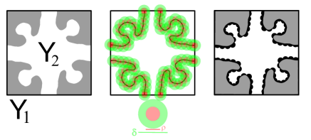
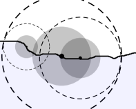
Idea of Proof: In order to highlight the structure of the following proof, let us explain how the extension operator is constructed. In Figure 2 we see on the left a Lipschitz surface with maximal Lipschitz constant , which can be locally covered by balls of radius (middle). Using the extension operators given by Lemma 2.2, we can extend to the red balls that intersect . The extension operators on the various red balls are then glued together using a suitable partition of unity. However, this leads to steep gradients in the black region on the right hand side, while in the white region. In particular, if is locally constant, these gradients are of order . Hence, proceeding globally in this way, the gradient cannot be bounded by .
To avoid this problem, in Step 2 we use a mesoscopic correction: Writing , and for with a partition of unity and the local extension operator on , we define the global extension operator through:
| (3.6) |
where for some suitable ball . By this, we assign to the void space an averaged value of the surrounding matrix. In Step 2 we heavily rely on the periodicity, which allows to apply a -periodic partitioning to .
Proof.
Step 1 (Local extension operator on ): W.l.o.g. we can assume that . Writing the set is precompact and can be covered by a finite number of balls , where and .
In what follows, let be a positive symmetric smooth function with on , and monotone on . We denote and for . In what follows we identify with their periodized versions. For every let and note that defines a partition of unity on . Writing for the corresponding extension operator from Lemma 2.2 on , we extend by to and consider
| (3.7) |
For the following calculation, we further note that
for some depending only on the dimension . Let . For every , the number of balls in intersecting with is bounded by . On each ball we infer from Lemma 2.2
Similar estimates also hold for and summing over , we obtain
| (3.8) | ||||
| (3.9) |
Now let be a ball with positive radius. By a contradiction argument, we obtain
| (3.10) |
and hence defining we find
| (3.11) |
Step 2 (gluing together the local extension operators): In what follows, for every let the operator shifted onto the cell . Given some positive with and symmetric w.r.t. the center of we write such that and introduce which provide a -periodic partition of unity. Note that at each at most functions are different from . We now define the operator according to (3.6) with and from Step 1 to find
| (3.12) |
In order to derive an estimate on , note that for and for all it holds by symmetry and hence (writing
Thus, let such that . Since is open and connected, one can prove
| (3.13) |
where depends on , and . Together with (3.9)–(3.11) we infer (3.5). Estimate (3.4) can be proved in an analogue way. ∎
4 Quantifying Nonlocal Regularity Properties of the Geometry
We have to account for three types of randomness. One is local, namely the local Lipschitz regularity. The other is of global nature: We have to find a partition of such that on each partition cell the extension can be explicitly constructed in a well defined way. In the case of periodicity this is evidently trivial. However, since we lack periodicity, we have to replace the periodic construction of the extension operator in Section 3 by something similar, but of stochastic nature. The key to this will be the local -regularity
The second problem will be overcome using a random distribution of balls within and a Voronoi tessellation which is such that every Ball is contained in exactly one Voronoi cell. This construction is based on the following observation.
Lemma 4.1.
Let be a stationary and ergodic random open set such that
Then there exists such that with positive probability the set contains a ball with radius .
Proof.
Assume that the lemma was wrong. Then for every the set almost surely does not contain an open ball with radius . In particular with probability the set does not contain any ball. Hence almost surely, contradicting the assumptions. ∎
The numbers and from Lemma 4.1 will finally lead to the concept of mesoscopic regularity of the geometry , see Definition 4.19. Particularly the number is important, as it affects also the construction of the extension operator on the very microscopic level.
The third problem is the hardest: It is the necessity to quantify connectedness of a domain geometrically and analytically.
4.1 Microscopic Regularity
Definition 4.2 (-Regularity).
Let be an open set.
-
1.
is called -regular in if and , i.e. there exists an open set and a Lipschitz continuous function with Lipschitz constant such that is graph of the function in some suitable coordinate system.
-
2.
is called locally -regular if for every there exists and such that is -regular in .
-
3.
is called (globally) -regular or minimally smooth if there exist constants s.t. is -regular in every .
The concept of (global) -regularity or minimally smoothness can be found in the book [35]. The theory of [35] was recently used in [13] to derive extension theorems for minimally smooth stochastic geometries. A first application of the concept of -regularity is the following Lemma, which is important for the application of the Poincaré inequalities proved in Section 2 during the construction of the local extension operators in Section 5.
Lemma 4.3.
Let be locally -regular. Then for every with the following holds: For every let such that is a Lipschitz manifold. Then there exists with such that with it holds .
Proof.
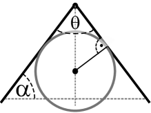
We can assume that is locally a cone as in Figure 3. With regard to Figure 3, for with and as in the statement we can place a right circular cone with vertex (apex) and axis and an aperture inside , where . In other words, it holds . Along the axis we may select with . Then the distance of to the cone is given through
In particular as defined above satisfies the claim. ∎
Continuity properties of , and
Our main extension and trace theorems will be proved for locally -regular sets and is based on some simple properties of such sets which we summarize in this section. Additionally we introduce the quantity .
Lemma 4.4.
Let , be a locally -regular open set and let such that for every there exists , such that is -regular in . Define for every
Then is -regular in the sense of Definition 2.11 with
In particular, is locally Lipschitz continuous with Lipschitz constant and for every and it holds
| (4.1) |
Remark 4.5.
The latter lemma does not imply global Lipschitz regularity of . It could be that and and are connected by a path inside with the shortest path of length . Then Lemma 4.4 would have to be applied successively along this path yielding an estimate of .
Proof of Lemma 4.4.
It is straight forward to verify that and satisfy the conditions of Lemma 2.12. ∎
With regard to Lemma 2.2, the relevant quantity for local extension operators is related to the variable , where is the related Lipschitz constant. While we can quantify in terms of and , this does not work for . Hence we cannot quantify in terms of its neighbors. This drawback is compensated by a variational trick in the following statement.
Lemma 4.6.
Let be locally -regular and let satisfy (4.1) such that is -regular. For and let be the Lipschitz constant of in and define
| (4.2) | ||||
| (4.3) |
Then, and are positive and locally Lipschitz continuous on with Lipschitz constant and is and -regular in the sense of Definition 2.11. In particular, for or it holds respectively
Remark 4.7.
For the same reason as in Remark 4.5. The latter lemma does not imply global Lipschitz regularity of or .
Proof.
Positivity is given by . Let and . For sufficiently large it holds implying is -regular. From here we conclude that is -regular and the above chain of inequalities follows from Lemma 2.12.
Lemma 4.8.
Let , be a locally -regular open set and let such that for every there exists , such that is -regular in . For let from Lemma 4.4 or or from Lemma 4.6 and define
| (4.4) | ||||
| (4.5) |
Then, for fixed , are upper semicontinuous and on each bounded measurable set the quantity
| (4.6) |
with if is well defined. The functions
are upper semicontinuous.
Remark 4.9.
In order to prevent confusion, let us note at this point that defined in (4.9) is different from . In particular, is a quantity on , while is a quantity on . Furthermore, as the last lemma shows, is upper semi continuous, while is only measurable.
Notation 4.10.
The infimum in (4.4) is a for . We sometimes use the special notation
Proof of Lemma 4.8.
Let with . Writing and and
as well as we observe from -regularity that and . Hence we find
Observing that as we find and is u.s.c.
Let . First observe that . The set is compact and hence in the Hausdorff metric as . Let such that . Since w.l.o.g. we find converges and . Hence
In particular, is u.s.c. The u.s.c of can be proved similarly. ∎
Corollary 4.11.
Let and let be a locally -regular open set, where we restrict by . Then there exists a countable number of points such that is completely covered by balls where . Writing
For two such balls with it holds
| (4.7) | ||||
| and |
Furthermore, there exists and such that and for .
Measurability and Integrability of Extended Variables
Lemma 4.12.
Proof.
Step 1: Let be a dense subset. If for some then also for sufficiently small, by continuity of . For every consider the function as introduced above. Then every is upper semicontinuous and is measurable. In particular, the set is measurable and thus is measurable.
Step 2: We show that for every the preimage is closed. Let be a sequence with . Let be a sequence with . W.l.o.g. assume and . Since is continuous, it follows . On the other hand and thus . ∎
Lemma 4.13.
Under the assumptions of Lemma 4.12 there exists a constant only depending on the dimension such that for every bounded open domain it holds
| (4.10) | ||||
| (4.11) |
Finally, it holds
| (4.12) |
Remark 4.14.
Proof.
Step 1: Given with let
| (4.13) |
Such exists because is locally compact. We observe with help of the definition of , the triangle inequality and (2.19)
The last line particularly implies (4.12) and
Step 2: By Theorem 2.13 we can chose a countable number of points such that is completely covered by balls where . For simplicity of notation we write and . Assume with given by (4.13). Since the balls cover , there exists with , implying and hence . Hence we find
Step 3: For with we can distinguish two cases:
and hence
Step 4: Let be fixed and define , . By construction, every with satisfies and hence if and we find and . This implies that
We further observe that the minimal surface of is given in case when is a cone with opening angle . The surface area of in this case is bounded by . This particularly implies up to a constant independent from :
The second integral formula follows in a similar way. ∎
4.2 Mesoscopic Regularity and Isotropic Cone Mixing
In what follows, we built upon Lemma 4.1 to motivate our definition of mesoscopic regularity (Definition 4.17 by the following two Lemmas.
Lemma 4.15.
Recall from Lemma 2.50 and assume . Let
then there exists a constant such that for almost every it holds for all regular convex averaging sequences
| (4.14) |
Remark.
Proof of Lemma 4.15.
Due to Lemma 4.1, with probability the set contains a ball and thus the set contains a ball . In particular, the stationary ergodic random measure has positive intensity . Let . Then there exists and thus there exists with . It follows
Since is stationary ergodic and is regular we find
∎
Lemma 4.1 suggests that starting at the origin and walking into an arbitrary direction, it is almost impossible to not meet a ball of radius that fully lies within . However, this is in general wrong, as for a given fixed direction one may already find periodic counter examples. In what follows, we will therefore use the weaker concept of isotropic cone mixing (Definition 4.17) which is based on the following observation:
Lemma 4.16.
Let be countable. Then for every and each there holds
Proof.
By stationarity, we can assume and by Lemma 4.15 the random measure has strictly positive intensity.
We write and denote by the cone with the same base as but with apex . Then is a regular convex averaging sequence. Furthermore, it holds implying as . Thus
where we use as . We infer that and hence the statement ( has to contain infinitely many balls ). ∎
The following definition is a quantification of Lemma 4.16.
Definition 4.17 (Isotropic cone mixing).
A random set is isotropic cone mixing if there exists a jointly stationary point process in or , , such that almost surely two points have mutual minimal distance and such that . Further there exists a function with as and such that with ( being the canonical basis of )
| (4.15) |
Criterion 4.18 (A simple sufficient criterion for (4.15)).
Let be a stationary ergodic random open set, let be a positive, monotonically decreasing function with as and let s.t.
| (4.16) |
Then is isotropic cone mixing with and with . Vice versa, if is isotropic cone mixing for then satisfies (4.16) with .
Definition 4.19 (Mesoscopic regularity).
A random set satisfying Criterion 4.18 is also called mesoscopically regular and is the regularity. is called polynomially (exponentially) regular if grows polynomially (exponentially).
Proof of Criterion 4.18.
Because of it holds for
The existence of implies that there exists at least one such that and we find
In particular, for and large enough we discover
The relation (4.15) holds with .
The other direction is evident. ∎
Note that Criterion 4.18 is much easier to verify than Definition 4.17. However, Definition 4.17 is formulated more generally and is easier to handle in the proofs below, that are all built on properties of Voronoi meshes.
The formulation of Definition 4.17 is particularly useful for the following statement.
Lemma 4.20 (Size distribution of cells).
Let be a stationary and ergodic random open set that is isotropic cone mixing for , , and . Then and its Voronoi tessellation have the following properties:
-
1.
If is the open Voronoi cell of with diameter then is jointly stationary with and for some constant depending only on
(4.17) -
2.
For let . Then
(4.18)
Proof.
1. W.l.o.g. let . The first part follows from the definition of isotropic cone mixing: We take arbitrary points . Then the planes given by the respective equations define a bounded cell around , with a maximal diameter which is proportional to . The constant depends nonlinearly on with as . Estimate (4.17) can now be concluded from the relation between and and from (4.15).
2. This follows from Lemma 2.15. ∎
Lemma 4.21.
Let be a stationary and ergodic random random points process with minimal mutual distance for and let be such that the Voronoi tessellation of has the property
Furthermore, let be measurable and i.i.d. among and let be independent from each other. Let
be the cell enlarged by the factor , let and let
where is a constant. Then is jointly stationary with and for every there exists such that
| (4.19) |
where
Proof.
We write , , , . Let
with . We observe that
| (4.20) |
which follows from the uniform boundedness of cells , and the minimal distance of . Then, writing for every it holds by stationarity and the ergodic theorem
In the last inequality we made use of the fact that every cell , , has volume smaller than . We note that for
Due to (4.20) we find
and obtain for and :
For the sum to converge, it is sufficient that for some . Hence, for such it holds and thus (4.19).
∎
4.3 Discretizing the Connectedness of -Regular Sets
Let be a stationary ergodic random open set which is isotropic cone mixing for , and . Then generates a Voronoi tessellation according to Lemma 4.20 with cells and balls . While the -regularity of is a strictly local property with a radius of influence of , the isotropic cone mixing is a mesoscopic property, with the influence ranging from to .
In this part, we close the gap by introducing graphs on that connect the small local balls covering with in . The resulting family of graphs and paths on these graphs will be essential for the last step in Section 7.
Definition 4.22 (Admissible and simple graphs).
Let with corresponding like in Corollary 4.11 and let be a countable set of points with and let be a graph. Then the graph on is admissible if it is connected and every has exactly one neighbor . An admissible graph is called simple if every has - besides - only neighbors in .
The following concept will become important later in Section . For reasons of self-containedness, we introduce it already at this point.
Definition 4.23 (Locally connected and ).
Assume that is an admissible graph on
with the property that for
with corresponding it holds
iff .
The
graph consists of all elements of , except
those for which there is no
path in or in
connecting with .
If is connected, the set is called locally
connected.
Locally flat geometries will turn out to be particularly useful as they allow to construct tubes around paths that fully lie within and connect the local with the mesoscopic balls.
Definition 4.24 (Admissible paths).
Let be an admissible graph on and let be a family of paths from to which are constructed from a deterministic algorithm that terminates after finitely many steps. Assume that for every . If is the radius of from Corollary 4.11 assume there exists
such that is invertible for every and . Then the family is called admissible.
A general approach to construct admissible graphs and paths on locally connected
For a particular family of random geometries, there might be sophisticated ways to construct and the families . However, it is interesting to know that such a graph can be constructed very generally for every locally connected geometry. In this section, we will thus introduce a concept how to transform the domain into such a graph, thereby bridging the gap between the local regularity of and the mesoscopic regularity. The basic Idea is sketched in Figure 4.
The grid
Let be open and . For let
| (4.21) |
and . Then we find the following:
Lemma 4.25.
Let be a connected open set which is locally -regular. For let be a family of points with a mutual distance of at least satisfying and let with corresponding and like in Corollary 4.11. Then there exists a family of points with such that with , and the family covers and
| (4.22) |
Furthermore, implies
| (4.23) |
i.e. . Finally, there exists such that for every
| (4.24) |
Notation 4.26.
Summing up and extending the notation of Lemma 4.25 we write
| (4.25) | ||||||||
The meaning of introducing the symbol will be clarified below.
For we write and for we use the above notation (4.21) and further define
| (4.26) |
We finally introduce the following bijective mappings
| (4.27) |
Proof of Lemma 4.25.
We recall and and that (4.7) holds. Furthermore, and hence for .
If we define and observe that is -regular (for defined in (4.21)). Then Lemma 2.12 and Theorem 2.13 yield a cover of by a locally finite family of balls , where , and where (4.22) holds. Looking into the proof of Theorem 2.13 we can assume w.l.o.g. that by suitably bounding .
Furthermore, we find for that
Next, for such we consider all such that and since for all such , we infer and hence by Lemma 4.6
Finally, follows from .
Definition 4.27 (Neighbors).
Under the assumptions and notations of Lemma 4.25, for two points let , . We say that and are neighbors, written , if . This implies a definition of “neighbor” for . For and we write if . We denote by , or simply the graph on generated by .
Remark 4.28.
a) Every has a neighbor .
b) Besides , points have no other neighbors.
The admissible paths
We will see below that is admissible if is connected. Besides we introduce further (reduced) graphs on , which are based on continuous paths. For two points we denote
Definition 4.29.
Using the notation of Lemma 4.25, the graph
is the subset of where all elements and are removed for which . Furthermore, if with has a neighbor such that and are not connected through a path which lies in , then , are removed.
We write for either , , or any other subset of which is connected.
Lemma 4.30.
Assume is connected, assume and . Then there exists such that is a path from to , for two points it holds either or or and there exist constants depending only on the dimension but not on or such that
We denote as .
Proof.
Let . If we infer from Lemma 5.2 below that . We recall that is a graph of a Lipschitz continuous function and that both and as well as lie below that graph. We project and as well as onto the sphere , which still do not intersect with the graph of . From here we may construct satisfying the claimed estimates. Since and and , we conclude that the constants can be chosen independently from .
If we can proceed analogously. ∎
Lemma 4.31 ( is admissible).
Under the assumptions and notations of Lemma 4.25 for every there exists a discrete path from to in .
Proof.
Since is connected, there exists a continuous path with , . Since is compact, it is covered by a finite family of balls , . If the statement is obvious. Otherwise there exists a maximal interval , , such that , and there exists such that for some . One may hence iteratively continue with on the interval . ∎
Hence, every two points in can be connected by a discrete path. However, the choice of the path is not unique, there might be even infinitely many with arbitrary large deviation from the “shortest” path. Luckily, it turns out that it suffices to provide a deterministically constructed finite family of paths.
Definition 4.32 (Admissible paths on ).
Let be open, connected and locally connected with such that the assumptions of Lemma 4.25 are satisfied. Let . We call any family of paths which connect to admissible, if it is generated by a deterministic algorithm that terminates after a finite number of steps. Hence, an admissible path from to in is a path with , generated according to this algorithm. We denote the set of admissible paths from to by .
Notation 4.33.
Let , and . Recalling (4.26), for we define the set of paths connecting , , … chosen as straight line if and from Lemma 4.30 else and
In what follows, we are usually working with the latter expression and hence introduce for simplicity of notation the identification . In this way, is an open set and the characteristic function is integrable as Lemma the next Lemma 4.38 will reveal. Finally, by Lemma 4.25 there exists such that independent from , and it holds
| (4.28) |
Construct a finite family
In what follows, we will construct a class of admissible paths on which does not rely on the metric graph distance. We study the discrete Laplacian on an admissible graph given by
It is well known that is a discrete version of an elliptic second order operator, see [4, 11, 17] and references therein. This may be quickly verified for the “classical” choice with iff (using Taylor expansion and the limit ).
The discrete Laplacian is connected to the following discrete Poincaré inequality.
Lemma 4.35.
Let be open, connected and satisfy the assumptions of Lemma 4.25, let be admissible and let . Writing
There exists and such that for every the following discrete Poincaré estimate holds:
| (4.29) |
Proof.
This is straight forward from a contradiction argument (using connectedness of ). ∎
For the following result we introduce the notation:
Lemma 4.36 (A discrete maximum principle).
Proof.
W.l.o.g. let and write iff . Using the notation of Lemma 4.35 and and we divide the proof in three parts.
Approximation: We consider the problem
| (4.32) |
Putting for and all , we find
| (4.33) |
which is a strictly positive definite bilinear symmetric form on . Hence, there exists a unique solution to (4.32).
Since is finite, attains a maximum and a minimum. If attains a local maximum in , it holds and if attains a local miminum in it holds . If attains negative values, it has a negative minimum in and hence , a contradiction. Thus, in every . Furthermore, because of (4.32) can attain a local maximum only in .
Passage : Using Lemma 4.35, for some large enough we find the following estimate, which holds for every due to (4.32) and (4.29) applied to
| (4.34) |
Together with (4.33), the latter yields a uniform estimate for all . In particular (due to a Cantor argument), there exists a subsequence such that converges for every as . Evidently, solves (4.30), is non-negative, attains its maximum in and satisfies the estimate (4.31). The limit as follows from (4.31) and (4.34). has a unique local maximum in for the same reason as for .
Uniqueness of : Finally, let and be two solutions such that satisfies
Multiplying the above equation with and summing over all , we find
which implies . ∎
Definition 4.37.
Let , let be the solution of (4.30) and . An admissible harmonic path from to in is a path with , such that . We denote the set of admissible harmonic paths from to by . If we simply write . Note that
Lemma 4.38.
Let be open, connected and satisfy the assumptions of Lemma 4.25. Let be admissible and let and . There exists , depending on , and such that every admissible harmonic path from to lies in . If are the natural numbers such that for every it holds (which exist due to Lemma 4.25) then we can choose
| (4.35) |
Proof.
Let us recall that for every by Lemma 4.36. Again we write if .
For an admissible path from to it follows for every . On the other hand
Let us further recall, that with and independent from . Given we can therefore conclude the necessary condition
On the other hand, it holds . This implies that the left hand side of the last inequality is bounded from below by
Hence we conclude (4.35) from
∎
The most important and concluding result in this context is the following, which states that the set of admissible paths is not empty and the is connected:
Theorem 4.39 (Admissible are connected through admissible harmonic paths).
5 Extension and Trace Properties from -Regularity
5.1 Preliminaries
For this whole section, let be a locally -regular open set and let be bounded by and satisfy (4.1). In view of Corollary 4.11, there exists a complete covering of by balls , , where . We define with , given in Lemma 4.6
| (5.1) |
and recall (4.8), which we apply to in order to obtain the measurable function
| (5.2) |
Similarly, in view of (4.9), we define the measurable function
| (5.3) |
Here we have used the convention .
Remark 5.1.
a) In view of Lemma 4.8 we recall Remark 4.9 on the difference between and and additionally remark that for every .
b) We could equally work with replacing . However, Lemma 4.6 suggests that the natural choice is .
Lemma 5.2.
For two balls either or and
| (5.5) |
Furthermore, there exists a constant depending only on the dimension and some such that
| (5.6) | |||||
| (5.7) | |||||
| (5.8) |
Finally, there exist non-negative functions and such that for : , for . Further, on all and on and and there exists depending only on such that for all , it holds and
| (5.9) |
Remark 5.3.
We usually can improve to at least . To see this assume is locally connected. Then all points lie on a -dimensional plane and we can thus improve the argument in the following proof to .
Proof.
Let be fixed. By construction in Corollary 4.11, every with satisfies and hence if and we find and . This implies (5.6)–(5.7) for and the statement for follows analogously.
For two points , such that it holds due to the triangle inequality . Let and choose such that is maximal. Then and every satisfies . Correspondingly, for all such . In view of (4.7) this lower local bound of implies a lower local bound on the mutual distance of the . Since this distance is proportional to , and since , this implies (5.8) with . This is by the same time the upper estimate on .
Let be symmetric, smooth, monotone on with and on . For each we consider a radially symmetric smooth function and an additional function . In a similar way we may modify such that for . Then we define . Note that by construction of and we find and on .
5.2 Extension Estimate Through -Regularity of
By Lemmas 4.6 and 2.2 the local extension operator
| (5.10) |
is linear continuous with bounds
| (5.11) | ||||
| (5.12) |
and for constants we find
| (5.13) |
Definition 5.4.
For two points and such that we find
| (5.15) |
The latter expression is not symmetric in . Hence we can play a bit with the indices in order to optimize our estimates below. We have seen that , and hence we expect in view of (5.11)
| (5.16) |
However, this needs not to be the optimal estimate. Instead of the general and restrictive estimate (5.16), we make the following Assumption:
Assumption 5.5.
There exists and such that for every it holds . In particular, for two points with it holds
| (5.17) |
In order to formulate our main results we define the general sets
| (5.18) |
and for every bounded set we define
| (5.19) |
Lemma 5.6.
The second term in (5.21) imposes severe problems, as we will see in Sections 7, 6.2 or even in Lemma 5.8 below.
Lemma 5.7.
Let , , , be a family of real numbers such that and let . Then
Proof.
∎
Proof of Lemma 5.6.
For shortness of notation (and by abuse of notation) we write
and similar for integrals over and .
Step 1: We note that as well as . The integral over can be estimated via
| (5.25) | |||
(5.9) together with Jensen’s yields
where we used Lemma 2.6 with and inequality (5.11). In a similar way, we conclude
It only remains to estimate . Inequality (5.8) yields
| (5.26) |
Step2: We now study and use Lemma 5.7 which yields
| (5.27) |
that
| (5.28) |
where
| (5.29) |
Since in (5.29) we obtain
We will now derive an estimate on . For this reason, denote the line from to and by the set of all points with distance less than to . We exploit the fact that every term in the sum on the right hand side of (5.28) appears only once and introduce
We make use of (5.17) and successively apply Jensen’s inequality, , and to obtain
Hence we find
| (5.30) |
Step 3: We observe with Jensen’s inequality and the fact that are linear with for constants that
From here we may proceed as in (5.26) to conclude . ∎
Lemma 5.8.
Proof.
We observe with Hölder and Jensens inequality on and in the sum respectively that
Applying the same trick again we find
From the definition of and (5.7) we find
∎
5.3 Traces on -Regular Sets
Theorem 5.9.
Let be a locally -regular open set, and let be a bounded open set and let . Then the trace operator satisfies for every
where for some constant depending only on , and and and for one may chose between
| (5.31) | ||||
| (5.32) |
Proof.
Using Theorem 2.13, we cover by balls with and define and . Like for (5.7) we can show that the covering with both and is locally uniformly bounded by a constant . Due to Lemma 2.4 we find locally
| (5.33) |
If is a partition of on with respective support we obtain
which yields by the uniform local bound of the covering, defined in Lemma 4.13, twice the application of (4.12) and (5.33)
With Hölders inequality, the last estimate leads to (5.31). The second estimate goes analogue since the local covering by is finite. ∎
6 Construction of Macroscopic Extension Operators I: General Considerations
In this section, we provide the extension results which answer the question of the existence of such uniformly bounded families of operators up to the issue of quantifying connectedness. We will discuss what we mean by that in Section 6.2. In Section 6.4 we provide a first attempt to from the point of view of continuous PDE, which is - in some sense - a tautology. However, verifying the conditions of Theorem 6.10 in a computer based approach (for real life geometries) leads to a discretization of an elliptic second order operator. Therefore, in Section 7 we use the construction of Section 4.3 to introduce a quantity which can be directly calculated from a numerical algorithm.
6.1 Extension for Voronoi Tessellations
Assumption 6.1.
Let be an open set and let have mutual distance if and with for every (e.g. , see (2.36)). We construct from a Voronoi tessellation and denote by the Voronoi cell corresponding to with diameter . We denote and
| (6.1) |
Let be monotone decreasing with , if and for . We define on the functions
| (6.2) |
Definition 6.2 (Weak Neighbors).
Under the Assumption 6.1, two points and are called to be weakly connected (or weak neighbors), written or if . For open we say if . We then define
| (6.5) |
Let be locally -regular and satisfy Assumption 6.1. Then we can construct continuous local extension operators from Lemma 5.6. These can be glued together via
However, using the partition of unity from Lemma 5.2 and the definition of from (5.14) we obtain
Using the latter yields
where we used that maps constants onto constants via the identity. Note that
as in most points.
Theorem 6.3 (Extensions for locally regular, isotropic cone mixing geometries).
Let the open set be locally -regular, bounded by , and satisfy Assumptions 5.5, 6.1 and be the constant from (5.8),. Let and with .
Recalling (5.4) and defining as well as
| (6.6) |
the following estimates hold:
| (6.7) | ||||
| (6.8) |
where
with functions
Proof.
From the last inequality and Lemma 5.6 we obtain (6.8). Furthermore, the first term on the right hand side of (6.9) with Lemma 5.6 provides the first line of (6.7).
In what follows, we write for simplicity but have in mind the respective meaning. The same holds for .
Concerning the second term in (6.9), we observe
and obtain with help of Lemma 5.7 and for
Similarly, we use Lemma 5.7 together with and find
where the first term on the right hand side can be estimated like in Lemma 5.6. Finally, from a similar calculation using Lemma 5.7 it is now obvious for the third term in (6.9) that
∎
6.2 The Issue of Connectedness
In Theorem 6.3 we discovered the integral as part of the estimate for , where we recall that was given through
We seek for an interpretation of the two sums appearing on the right hand side. The first one is related to the difference of mean values around and in case they are weak neighbors, i.e. . In Theorem 6.7 below we provide a rough estimate on this part in terms of but on a larger area. In the present section, we first want to “isolate” and from the other geometric properties of . In Section 7 we will see how these quantities are related to the connectivity of .
Lemma 6.4.
Proof.
We find from Hölder’s and Jensen’s inequality
The other inequality can be derived similarly, see also the proof of Lemma 5.8. ∎
Proof.
For this we observe with help of (6.4) and with Lemma 4.20.2)
| (6.11) | ||||
| (6.12) |
We write
and find
Now we make use of (6.11) and once more of Lemma 4.20.2) to obtain for the first bracket on the right hand side an estimate of the form
which implies
where we used . We make use of in the above estimates and Hölder’s inequality to find
Since for some independent from , we obtain
∎
6.3 Estimates Related to Mesoscopic Regularity of the Geometry
Assumption 6.6 (Mesoscopic Regularity).
Theorem 6.7 (Extensions for mesoscopic regular, isotropic cone mixing geometries).
Remark 6.8.
A combination with Lemma 6.4 is possible.
Proof.
We make use of (6.3) as well as the following observation: for each let . Then
Hence
Given we hence find an estimate by
Next, we obtain
and thus
where according to Lemmas 2.6 and 5.6 for some depending only on and :
We integrate with respect to and obtain with
| (6.15) | |||
For the measurable function on we find for every
| (6.16) |
For the remaining expression note that
| (6.17) |
We denote the right hand side of (6.17) by . Using we obtain from Hölder’s inequality together with Jensen’s inequality
| (6.18) |
where and are defined in the statement and where we used and .
6.4 Extension for Statistically Harmonic Domains
Definition 6.9.
A random geometry is statistically -harmonic if there exist constants , and sets such that for every
Theorem 6.10.
Let be a stationary ergodic random open set which is -regular, isotropic cone mixing for and , statistically -harmonic and let Assumption 6.6 hold. Then for every and and every it holds
Proof.
We make use of on as well as the definition of to obtain that the latter expression is bounded by (compare also with the calculation leading to (5.16))
We use that are mutually disjoint and to find
7 Construction of Macroscopic Extension Operators II: Admissible Paths
In this section, we will use admissible paths on connected sets in order to estimate the (so far uncontrolled) terms in Theorems 6.3 and 6.7 in terms of .
Knowing there exists an admissible path (by Theorem 4.39), it remains to deal with the non-uniqueness of the path. Note there is no clear distinction which puts one path in favor of others. While this could be seen as a drawback, it can also be considered as an opportunity, since it allows to distribute the “weight” of integration along the paths more uniformly among the total volume. This is the basic idea of this section.
7.1 Preliminaries
Given an open connected set and a countable family of points satisfying Assumption 6.1 we extend the covering resp. of from Section 5.1 (e.g. (5.1)) to the inner of using Lemma 4.25. In this context, we remind the reader of (4.25) and Definition 4.27 and introduce the notation
We find the following
Lemma 7.1.
There exists independent from such that for every
Proof.
For two points such that it holds due to the triangle inequality
| (7.1) |
Let and choose such that is maximal. Then by (7.1) and every satisfies (Lemma 2.12). In view of (4.7) this lower local bound of implies a lower local bound on the mutual distance of the . Since this distance is proportional to , and since , this implies for some constant independent of or that
Now let and . We show
For the first inequality, observe that is equivalent with and hence
For the second inequality, assume . Then lies closer to the boundary than and implies
The mutual minimal distance of neighboring points in terms of now implies for some independent from and
∎
Definition 7.2.
Let be a connected sub-graph of . Let and be the solution of the discrete Laplace equation (4.30) for on the graph . For every let
the neighbors corresponding the outgoing branches of admissible paths through , and we assign to each the weight of the branch where either
For we define the weight of the path by
Remark 7.3.
We observe
This holds by induction along the path and different branches since in every it holds .
7.2 Extension for Connected Domains
In this section, we discuss how the graphs built in Section 4.3 can be used to derive estimates on given in Theorem 6.3. The remaining constant on the right hand side is given in terms of the balls and length of the paths between and or and respectively. Although one could go even more into details and try to generally decouple these effects, this is not helpful for our examples in Section 8 below. Hence we leave the results of this section as they are but encourage further investigation in the future.
The idea
We first consider the case of a general graph on and do not claim that paths in the classes are fully embedded into . In particular, we drop for a moment the concept of local connectivity and we allow paths to intersect with . Let , and . In the following short calculation, one may think of as a function related to , though the following calculations will reveal that it is not exactly what we mean. Nevertheless, recalling Notation 4.33 for and it holds
| (7.2) |
Since is related to , the latter formula reveals that the terms may lead to an “entanglement” of and the properties of the paths . In what follows, we will resolve the latter calculation in more details to prepare this discussion.
In what follows, we will make use of and
and we write for the straight line segment connecting with . We distinguish 4 cases:
Case : According to Lemma 5.2 it holds and if is the corresponding local extension operator it holds
Case , : According to Lemma 4.25 it holds and if is the corresponding local extension operator it holds
Case , : According to Lemma 4.25 it holds and if is the corresponding local extension operator it holds
Case : According to Lemma 4.25 it holds and
However, in case of local connectivity, we face a simpler situation. In case we can use the above estimates while in the other cases, we can use the Lemma 4.30.
Locally connected
In what follows, we consider (see Definition 4.29) with a suitable family of admissible paths , and we also recall from Notation 4.33. We repeat the calculations of (7.2) in view of Lemma 4.30. In particular, if are connected via a path in , which additionally has the property that the corresponding tube exists, then the length of is bounded by , where is determined by the dimension. Hence we have
| (7.3) |
The last calculation is at the heart of the results in this section. In what follows, we adopt the situation of Lemma 6.4:
Lemma 7.4.
Proof.
We find
which leads to the result. ∎
And finally, we provide an estimate for the remaining term in Lemma 6.5. The proof is similar to the last Lemma.
7.3 Statistical Stretch Factor for Locally Connected Geometries
Definition 7.6.
Theorem 7.7.
Let the Assumptions of Theorem 6.3 hold and let be locally connected. . For every let
Defining and
| (7.4) |
it holds
where for some
Definition 7.8.
We call the statistical stretch factor.
Corollary 7.9.
It holds .
Corollary 7.10.
If satisfies on then has support on .
Proof.
This follows since
∎
Proof of Theorem 7.7.
Finally, the following result allows us to estimate the difference of and .
Theorem 7.11.
Remark 7.12.
Condition (7.5) is satisfied if e.g. for some as then
Proof.
Since we have to estimate the excess mass of over . If we define
we find
and we thus derive an estimate on the contribution from and respectively.
Let . Then for
Due to the ergodic theorem, we obtain for every
and similarly
Since the above estimates hold for every and every , we find
In a similar way, we prove
∎
8 Sample Geometries
8.1 Boolean Model for the Poisson Ball Process
Recalling Example 2.36 we consider a Poisson point process with intensity (recall Example 2.36). To each point a random ball is assigned and the family is called the Poisson ball process. We then denote and seek for a corresponding uniform extension operator. The following argumentation will be strongly based on the so called void probability. This is the probability to not find any point of the point process in a given open set and is given by (2.34) i.e. .
The void probability for the ball process is given accordingly by
which is the probability that no ball intersects with .
Theorem 8.1.
Remark 8.2.
We observe that the union of balls has better properties than the complement.
Proof.
We study only since is the complement sharing the same boundary. Hence, in case , all calculations remain basically the same. However, in the first case, we assume that , which we cannot assume in the other case, where is proportional to . This is the reason for the different in the two cases.
In what follows, we use that the distribution of balls is mutually independent. That means, given a ball around , the set is also a Poisson process. W.l.o.g. , we assume with . First we note that if and only if , which holds with probability . This is a fixed quantity, independent from .
Now assuming , the distance to the closest ball besides is denoted
with a probability distribution
It is important to observe that is -regular in the sense of Lemma 2.12. Another important feature in view of Lemma 4.4 is . In particular, and is -regular in case . Hence, in what follows, we will derive estimates on , which immediately imply estimates on .
Estimate on : A lower estimate for the distribution of is given by
| (8.1) |
This implies that almost surely for
i.e. .
Intersecting balls: Now assume there exists , such that . W.l.o.g. assume and . Then
and is at least -regular. Again, a lower estimate for the probability of is given by (8.1) on the interval . Above this value, the probability is approximately given by (for small i.e. ). We introduce as a new variable and obtain from that
| (8.2) |
No touching: At this point, we observe that is almost surely locally finite. Otherwise, we would have and for every we had . But
Therefore, the probability that two balls “touch” (i.e. that ) is zero. The almost sure local boundedness of now follows from the countable number of balls.
Extension to : We again study each ball separately. Let with tangent space and normal space . Let and such that , then also and and by Lemma 2.12. Defining
we find
Studying on we can assume in (4.10) and we find
Hence we find
Estimate on : For two points let and . For the fixed ball we write and obtain with from (8.2). Therefore, we find
We now derive an estimate for
To this aim, let . Then implies and
The only random quantity in the latter expression is . Therefore, we obtain with that
Since the point process has finite intensity, this property carries over to the whole ball process and we obtain the condition in order for the right hand side to remain bounded.
Estimate on : We realize that . Hence we obtain from Hölder’s inequality
where and . From the right hand side of the last inequality, we infer boundedness of the first expectation value for implying . Since we have to require , this implies and . On the other hand, we know that the second expectation is finite if . For , we obtain the lower bound for and hence we conclude the sufficient condition
which implies our claim.
Estimate on : We have to estimate the local maximum number of overlapping in a single point in terms of . We first recall that . Thus large discrepancy between and occurs in points where is large. This is at the intersection of at least two balls. Despite these “cusps”, the set consists locally on the order of of almost flat parts. Arguing like in Lemma 5.2 resp. Remark 5.3 this yields .
Estimate on : Given two points with radii , , and we find
By our initial assumptions on we prove our claim on . ∎
It remains to verify bounded average connectivity of the Boolean set or its complement. In what follows we restrict to the Boolean set and use the following result.
Theorem 8.3.
[37]Let have a connected component and let be the graph on constructed from iff . Let be the connected component of and . For let be the graph distance. Then for every there exists , such that
The latter result enables us to prove the following.
Lemma 8.4.
Using the notation of Theorem 8.3, let and . Then
In other words, the probability that the distance between and on the grid is stretched by more than is decreasing exponentially in .
Proof.
Let . Let and let such that . With probability there exists . For such it holds
In particular, we obtain for
Hence, assuming we find that at least one of the conditions or has to hold, which implies
Now it holds under the condition that exists
which implies the statement. ∎
We construct a suitable graph . For this we choose according to Lemma 2.50 and define
For and we choose the standard neighborhood relation. Furthermore, we say for and that iff there exists with and for , we say iff . This graph is called .
Theorem 8.5.
Let be the connected component of . Then is locally connected and for we find for every that .
Proof.
We write . Let with diameter of the Voronoi cell and let . We can chose with such that . Note in particular, that . Now let and let . If , then and, w.l.o.g., . For the graph distances it holds
In case we conclude with . If we obtain .
Hence, because , it only remains to observe that Lemma 8.4 yields an exponential decrease for the probability of large stretch factors for . ∎
8.2 Delaunay Pipes for a Matern Process
For two points , we denote
the cylinder (or pipe) around the straight line segment connecting and with radius .
Recalling Example 2.36 we consider a Poisson point process with intensity (recall Example 2.36) and construct a hard core Matern process by deleting all points with a mutual distance smaller than for some (refer to Example 2.37). From the remaining point process we construct the Delaunay triangulation and assign to each a random number in in an i.i.d. manner from some probability distribution . We finally define
the family of all pipes generated by the Delaunay grid “smoothed” by balls with the fix radius around each point of the generating Matern process.
Since the Matern process is mixing and is mixing, Lemma 2.22 yields that the whole process is still ergodic.
Remark 8.6.
The family of balls can also be dropped from the model. However, this would imply we had to remove some of the points from for the generation of the Voronoi cells. This would cause technical difficulties which would not change much in the result, as the probability for the size of Voronoi cells would still decrease subexponentially.
Lemma 8.7.
is a point process for that satisfies Assumption 6.1 and is isotropic cone mixing for with exponentially decreasing . Furthermore, assume there exists such that , then for some .
Proof.
Isotropic cone mixing: For the events and are mutually independent. Hence
Hence the open set is isotropic cone mixing for with exponentially decaying .
Estimate on : There exists such that is -regular in every . Since the distribution of is independent from and , this implies that .
Estimate on the distribution of : By definition of the Delaunay triangulation, two pipes intersect only if they share one common point .
Given three points with and , the highest local Lipschitz constant on is attained in
It is bounded by
where in the following denotes the angle between and , see Figure 6. If is the diameter of the Voronoi cell of , we show that a necessary (but not sufficient) condition that the angle can be smaller than some is given by
| (8.3) |
where is a constant depending only on the dimension . Since for small we find , and since the distribution for decays subexponentially, also the distribution for decays subexponentially.
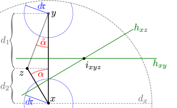
Proof of (8.3): Given an angle and we derive a lower bound for the diameter of such that for two neighbors of it can hold . With regard to Figure 6, we assume .
Writing the diameter of and , w.l.o.g let , where and . Hence we can assume that takes the form and in what follows, we focus on the first two coordinates only. The boundaries between the cells and and and lie on the planes
respectively. The intersection of these planes has the first two coordinates
. Using the explicit form of , the latter point has the distance
to the origin . Using and we obtain
Given , the latter expression becomes small for small, with the smallest value being . But then
and hence the distance becomes
We finally use and obtain
The latter expression now needs to be smaller than . We observe that the expression on the right hand side decreases for fixed if increases.
On the other hand, we can resolve . From the conditions and , we then infer (8.3). ∎
Lemma 8.8.
Proof.
Since the admissible paths are the shortest paths, there exists such that for every , , it holds . Furthermore, for with we find and since and are connected through a path lying inside possibly crossing other we can assume for the same that for every , it holds . This provides a uniform bound on . The lemma now follows from Lemma 4.21 and Theorem 7.11. ∎
9 Sobolev Spaces on the Probability Space
Based on Assumption 2.14, we want to achieve a better understanding of the mapping . For this we make the following basic assumption throughout this section.
Assumption 9.1.
For the introduction of traces of -functions below we will need the following (uncommon) stronger assumption. It is motivated by Theorem 2.33, which states that we can assume to be a separable metric space.
Assumption 9.2.
Assumption 9.2 will pay of due to the second part of the following lemma, which is a fundamental property of separable -algebras.
Lemma 9.3.
Let be a measure space with a countably generated -algebra . Then for every the space is separable. If is a separable metric space and the completion of the Borel algebra with respect to then densely and continuously, where are the bounded continuous functions on .
The following lemma is a fundamental observation which will be frequently used throughout the rest of this work. It relies on the following notation. For , a metric space, and we define the realization of as
Then we find the following behavior.
Lemma 9.4.
Let Assumption 9.1 hold and let for . Then for almost every and for every bounded domain it holds .
Proof.
For observe that
From Fubini’s theorem it follows that exists for a.e. . For the statement follows since exists for every . ∎
9.1 The Semigroup on and its Generators
For every we define the mapping
through . This mapping is well defined for every measurable function . Moreover, we have the following properties.
Lemma 9.5.
Let Assumption 9.1 hold. For every , the family is a strongly continuous unitary group on .
Proof.
Every is linear on and the group property follows from . Since is measure preserving, we find and hence is unitary.
In order to prove the strong continuity, observe
where we used that preserves measure and Fubini’s theorem. By Lemma 9.4 for almost every and for such it holds . Furthermore, for we have
Thus, the Lebesgue dominated convergence theorem yields
∎
For , let be the -th canonical basis vector in . Since define a strongly continuous group we can draw the conclusion that the operators , define independent one-parameter strongly continuous semigroups on that commute with each other and jointly generate on . Each of these one-parameter groups has a generator defined by
The expression is called -th derivative of and is skew adjoint:
The joint domain of all in is denote
with the natural norm
In case , this is a Hilbert space with scalar product
We finally denote the gradient with respect to and by the adjoint of . Sometimes we write to underline the gradient aspect. Similar to distributional derivatives in , we may define through iterated application of and
In case Assumption 9.2 holds, we denote
Lemma 9.6.
For every for almost every it holds . In particular, for every bounded domain it holds
| (9.1) |
Proof.
Let and let , . Using Lebesgue’s dominated convergence theorem it follows:
Since preserves measure, we obtain
Using a countable dense subset , and a suitable family of testfunctions , we obtain that for almost every equation (9.1) holds for every . Hence, by density, it holds for all . ∎
Lemma 9.7.
Let and let . For every let
Then for every it holds with and almost every realization of is an element of . Furthermore, the estimates
| (9.2) |
hold and we have .
Proof.
Let and observe
Due to the convolution inequality we have
and since is arbitrary, the we obtain , the first part of (9.2).
In order to show observe
Taking the limit in on both sides using Lebesgue’s dominated convergence theorem implies
| (9.3) |
and hence with and the second part of (9.2) follows. Equation (9.3) also shows that
and hence almost every realization of has -regularity. Furthermore, (9.3) implies
where we used continuity of and strong convergence of . ∎
Similar to - and Sobolev spaces on , we can introduce a family of smoothing operators. Let be a standard sequence of mollifiers which are symmetric w.r.t. and define
| (9.4) |
Lemma 9.8.
For every , , the operator is unitary and selfadjoint. For every , it holds , strongly in , and almost every realization of is an element of . Finally, for it holds
| (9.5) |
and .
9.2 Gradients and Solenoidals
We denote by the set of measurable functions such that for every bounded domain and we define
Remark 9.9.
The space is invariant under convolution. This follows immediately from the fact that if locally, then .
Recalling the notation for a realization for , we can then define corresponding spaces on through
| (9.6) | ||||
The spaces and are connected as the following theorem shows.
Theorem 9.10.
For with the spaces and are closed and it holds
| (9.7) |
in the sense of duality. Furthermore, lies densely in and
| (9.8) |
Proof.
The density of in follows from Lemma 9.8. We furthermore observe that is invariant with respect to . In fact, let and consider such that . Then
and hence due to Remark 9.9. Furthermore, the space is closed as can be seen from the continuity of the expression
where and are arbitrary.
Step 1: We first show that and are mutually orthogonal in the sense of duality. Let and and chose such that for , and the ergodic theorem LABEL:thm:Main-ergodic_Theorem_-_extended holds. Thus, we get weakly in . It remains to show that . Since , we find for every some such that and . By the ergodic theorem and has average . Due to the Poincaré inequality and the compact embedding , we find strongly in . Therefore, for all , we find
Therefore, we obtain
| (9.9) |
Step 2: We prove (9.7) and closedness of in case . From Step 1 we know that and it remains to show that . Let and use the decomposition where and . Since is symmetric and is invariant with respect to , we observe that
and hence . In particular, for every and every it holds
and as it holds
Since was arbitrary, this implies almost everywhere, i.e. . Since as , the closedness of implies . Hence and Step 1 implies and closedness of .
Step 3: For we deduce from Step 2
| (9.10) |
Interchanging the role of and yields
| (9.11) |
9.3 Stampaccia’s Lemma
Lemma 9.11 (Stampaccia).
Let be Lipschitz continuous and let . Then .
Proof.
Let . It holds
Hence, we find that there exists such that weakly along a further subsequence. Testing this limit with a function , we obtain that is the weak derivative of as
∎
Remark 9.12.
Theorem 9.13.
For every the embedding is dense. In particular,
Proof.
The last Theorem has an important implication for the existence of suitable countable and dense family of functions.
Theorem 9.14.
Let Assumption 9.1 hold. For every there exists a countable dense family of functions such that and is stable under addition and scalar multiplication with . Furthermore, every has almost surely bounded and continuously differentiable realizations with . If additionally Assumption 9.2 holds, then can be chosen such that for every it holds , .
Proof.
Let be dense. Then for every consider and for define . Then . Moreover, for every and every there exists with , with and with . Based on the countable family , we find that
satisfies all demanded properties.
If Assumption 9.2 holds we find dense in . For every like above and every we observe by Lemma 9.7 that
Hence the family is countable and dense . From here we can proceed similarly with the modification that are already in . Based on the countable family , we find that
satisfies all demanded properties.
The bound and continuous differentiability of realizations are a direct consequence of the construction of . ∎
9.4 Traces and Extensions
For the remainder of this section, we make the following assumption.
Assumption 9.15.
We then introduce the following function spaces.
Definition 9.16.
Under the Assumption 9.15 we introduce for the space
Based on Definition 9.16, we also introduce the following properties of and .
Definition 9.17.
We say for the corresponding prototypes in the sense of Theorem 2.33 that
-
1.
has the weak -extension property for if Assumption 9.1 holds and there exists a continuous linear operator such that . In this context, we define
-
2.
has the strong -extension property for if Assumption 9.1 holds and there exists a continuous linear operator such that and such that
-
3.
has the strong -trace property for if Assumption 9.2 holds and there exists a continuous linear operator such that for every it holds in the sense of .
We already mention at this point a very important property which holds for , but which we are not able to reproduce for general in this work. Hence we formulate it as a conjecture, and will avoid to use it in the remainder of this work. Fortunately, it turns out to be non-essential up to uniqueness properties of the homogenized problem in Section 10.6.
Conjecture 9.18.
If has the strong extension property it holds
Theorem 9.19.
In order to prove Theorem 9.19 we first need the following lemma.
Lemma 9.20.
Let Assumption 9.1 hold and let , then there exists a family which is dense in . If Assumption 9.2 holds then we can additionally assume . In both cases is stable under addition and scalar multiplication with . Furthermore, every has almost surely bounded and continuously differentiable realizations with
Proof.
Proof of Theorem 9.19.
A generalization of Theorem 9.19 to the general case of Assumption 9.1 is difficult, since the trace property does not apply for general -functions, even in . However, for the sake of homogenization, there exists a workaround.
Definition 9.21.
Theorem 9.22.
Proof.
We define pointwise in through and observe that is bounded by the argument in the proof of Theorem 9.19. It thus remains to show that is measurable, because then, we can simply extend to .
We will now turn our focus to the extension properties. We start with an important implication by the strong extension property.
Theorem 9.23.
Let Assumption 9.1 hold, let be ergodic and let have the strong -extension property. Then the operator can be extended to a continuous operator . More precisely we can identify with
This means that for and it holds iff .
Proof.
The first part follows immediately from the definition of the spaces and of the strong extension property.
For the second part, remark that and . Furthermore, is dense in by Lemma 9.20. Finally, and for and it holds iff . ∎
Theorem 9.24.
Theorem 9.25.
9.5 The Outer Normal Field of
Theorem 9.26.
Let Assumptions 9.2 and 9.15 hold and let have the strong -trace property for . Let be ergodic, let be almost surely locally -regular and let be the outer normal of on . Then there exists a measurable function such that almost surely . Furthermore, for and it holds
| (9.12) |
If satisfies the weak -extension property, the equation (9.12) extends to and or to and .
Proof.
For define . We observe that
| (9.13) |
and hence for almost every we have weakly. Then for and it holds by the Palm formula and (9.13)
where . From the ergodic theorem, the -almost sure pointwise weak convergence and the Lebesgue dominated convergence theorem, we conclude
which implies . In a similar way, we show , where is a -valued measure on . Furthermore, for every in the canonical basis of , , which implies by the Radon-Nikodym theorem the existence of a measurable with values in such that . The property follows from the fact that is the Palm measure of .
Definition 9.27.
Let have the strong -Trace property for and the weak -extension property. We say that has the weak normal trace and weak divergence if for all
Theorem 9.28.
Let Assumptions 9.2 and 9.15 hold and for some let have the strong -Trace property and the weak -extension property and let have the strong uniform trace property (see Definition 10.10 below). Let be ergodic, let be almost surely locally -regular and let be the outer normal of on . Then there exists , such that has a weak normal trace and weak divergence , i.e.
The last theorem is less trivial than one might think. In particular, we lack a Poincaré-type inequality on , which is typically used to prove corresponding results in . We shift the proof to Section 10.5.
10 Two-Scale Convergence and Application
As we have already explained in the introduction, there have been several approaches to the introduction of two-scale convergence in stochastic homogenization. In this work, we chose a modification of [16] because it does not rely on compactness of the underlying probability space.
10.1 General Setting
For the rest of this work, we consider a stationary random measure with Palm measure and we define
| (10.1) |
For the corresponding Lebesgue spaces we write or , where is a convex domain with -boundary. If , i.e. , or we omit the notion of and .
In our applications, for the characteristic function of the prototype of the random set with Palm measure or , with Palm measure located on , the prototype of . If we explicitly study the latter case, we write for the Palm measure.
Moreover, in view of (10.1), we write . In case of , we drop the notation .
Assumption 10.1.
Remark.
In some proofs below we will assume w.l.o.g. that some particular, essentially bounded functions are elements of . These will always be countably many and hence has to be changed only by a set of measure .
Definition 10.2.
Let Assumption 10.1 hold. Let and let for all . We say that converges (weakly) in two scales to and write if and if for every , there holds with
We note that the definition of two-scale convergence in [16] is formulated more generally, in particular for a more general class of test-functions.
Lemma 10.3 ([16] Lemma 4.4-1.).
Let Assumption 10.1 hold. Let and be a sequence of functions such that for some independent of . Then there exists a subsequence of and such that and
| (10.2) |
Sketch of proof.
Furthermore, we will need the following result on the lower estimate in homogenization of convex functionals using two-scale convergence, which was obtained in [18].
Lemma 10.4.
Let Assumption 10.1 hold and let be a random measure. Let be a convex functional in . For almost all the following holds: Let be a sequence such that for some and such that . Then, it holds
10.2 The “Right” Choice of Oscillating Test Functions
In what follows, we will have to deal with two-scale limits of functions on , but also on or . Hence we deal with two-scale convergence w.r.t. to , and . In order to keep notation of the set(s) of testfunctions short and concise, we make the following choice:
is the set countable set of functions from Theorem 9.14. Hence is dense in and is dense in (see Theorem 9.10).
10.3 Homogenization of Gradients
In what follows, we introduce two-scale convergence of gradients. This result has been proven in various work under various assumptions, see e.g. [2] for the periodic case and [39, 29, 16] in the stochastic case. We provide the proof here for self-containedness of this outline.
Theorem 10.5.
Under Assumption 10.1 for almost every the following holds:
If for all and if there exists with
Then there exists such that . Depending on the choice of , the following holds:
-
1.
If , then with weakly in and there exists such that weakly in two scales.
-
2.
If then for some .
-
3.
If then and .
-
4.
If then .
Lemma 10.6.
Under Assumption 10.1 for almost all the following holds: Let and be a sequence of functions satisfying
| (10.3) |
If along a subsequence, then is independent of .
Proof.
We obtain that along a subsequence. We show that does not depend on the -coordinate using ergodicity. We recall that are all measure preserving for . Hence, for any and , we find for any it holds
The first integral on the right hand side can be easily estimated through
The second integral can be estimated through
Due to (10.3) the right hand side of the above inequality converges to . Since and were arbitrary, we obtain for every . Hence is invariant under all translations , which implies for almost every that by ergodicity of . ∎
Proof of Theorem 10.5.
We note that and along a subsequence.
Proof of 1: We consider a countable set which is dense in . Then, by definition of we find for all and all
We take the limit on the left hand side and obtain
After integration by parts, this implies
As and were arbitrary and since is dense, the last equation and Lemma 9.10 imply that for almost every .
Proof of 2: We apply Part 1 to . Evidently, and hence there exists such that .
Proof of 3: Let and . Then we have
As we obtain
and since this holds for every and , we obtain that . Furthermore, for a countable dense family and we obtain
and in the limit
This implies .
Proof of 4: Part 3 implies that satisfies and . ∎
Important in the context of convergence of gradients is also the following recovery lemma, obtained in [15, Section 2.3] for the -case.
Lemma 10.7.
Let Assumption 10.1 hold. Let , and let be a bounded convex domain. For almost every there exists such that the following holds: For every there exists a unique with , and for all . Furthermore,
Sketch of Proof, see [15].
By definition of there exists for almost every a function with , . By a standard contradiction argument, there exists a constant such that
The last inequality implies that weakly in and strongly in . Furthermore, the Ergodic Theorem 2.26 yields for every
Hence and since it follows . ∎
10.4 Uniform Extension- and Trace-Properties
For the rest of this section, we make the following assumptions. Under the Assumptions 9.1 and 10.1 and using the notations introduced in Section 10.1 we introduce , and .
Following (10.1) we recall the definition
Definition 10.8 (Uniform Dirichlet extension property).
Let be a bounded open convex domain with Lipschitz boundary. We say for that has the uniform -Dirichlet extension property on if for almost every there exists and a linear extension operator
such that
satisfies the following: For every
and
| (10.4) |
Theorem 7.11 shows that virtually every random geometry to which the theory of Sections 5–7 applies has the - extension property on bounded convex -domains . In particular, we obtain the following reformulation of Theorem 1.9.
Theorem 10.9.
Proof.
There exists a weaker notion of extension property, which is for some applications sufficient.
Definition 10.10 (Uniform weak extension property).
Let be a bounded open convex domain with Lipschitz boundary. We say for that has the uniform weak -extension property on if for almost every there exists and a linear extension operator
such that
satisfies the following: For every
Theorem 10.11.
Proof.
After rescaling, this is the statement of Theorem 1.6. ∎
Similarly to the extension property, we may introduce a uniform trace property.
Definition 10.12 (Uniform trace property).
Let be a bounded open convex domain with Lipschitz boundary. We say for that has the uniform -trace property on if for almost every there exists such that the trace operators
satisfy the estimate
Theorem 10.13.
Proof.
After rescaling, this is the statement of Theorem 1.4. ∎
10.5 Homogenization on Domains with Holes
In what follows, we will naturally deal with two-scale limits of functions defined solely on . Hence we introduce the following definition.
Definition 10.14.
Let and for all . We say that converges (weakly) in two scales to and write if and if for every and there holds with
The latter definition coincides with Definition 10.2 for , which can be verified using the ergodic theorem. Hence, we find the following lemma:
Lemma 10.15.
Let and be a sequence such that . Then there exists and a subsequence such that .
Furthermore, if is a sequence such that and along a subsequence for some , then .
Proof.
This follows immediately from Lemma 10.3 extending by to and on noting that implies w.l.o.g. . ∎
Lemma 10.16.
Let be a random open domain such that has the weak uniform -extension property on for . Then for almost every the following holds: If for all with
for independent from then there exists a subsequence denoted by and a function such that
| (10.5) |
as well as
| (10.6) |
as .
Proof.
We are now able to provide the:
Proof of Theorem 9.24.
Theorem 10.11 shows that satisfies the uniform weak extension property. Hence, if is a countable dense subset of , we find a set of full measure such that for every and every the realizations are well defined elements of , the extension operator defined in (5.14) is uniformly bounded and hence defined in Definition 10.10 is uniformly bounded, too. We can thus use the two-scale convergence method as a tool.
Given such , we define and by Lemma 10.16 we find such that and . Furthermore, we find
Since the operator is linear and bounded, it can be extended to the whole of . ∎
Proof of Theorem 9.28.
For every there exists a unique that solves
Deriving apriori estimates in the usual way, for some independent from it holds
and thus according to Lemma 10.16 we find such that
along a subsequence which we again denote in the following, for simplicity. But then for and it follows
Since the left hand side of the above calculation converges to and was arbitrary, we conclude. ∎
Proof of Theorem 9.25.
Let and let with , . According to Theorem 10.9, has the uniform -Dirichlet extension property. The theorem now follows from part 2 of the following Lemma. ∎
Lemma 10.17.
Let be a random open domain such that has the uniform -Dirichlet extension property on for . Then for almost every the following holds:
-
1.
If for all with for independent from then there exists a subsequence denoted by and functions and such that
(10.8) (10.9) Furthermore, weakly in .
-
2.
has the strong -extension property with for .
-
3.
If and the Assumptions of Theorem 9.28 are satisfied and additionally has the uniform -trace property for some then
If, even further, has the uniform -trace property with from Part 1, then
(10.10)
Proof.
In what follows, convergences always hold along subsequently chosen subsequences of , which we always relabel by .
Proof of 1: Let . Then Theorem 10.5 and the assumption that (w.l.o.g.) yields that for some and
Proof of 2: For with we find for almost every that from Definition 10.8 satisfies
| (10.11) | ||||
As , Lemma 10.16 yields , , where . Moreover, inequality (10.11) implies in the limit that
Hence we can set . By density, this operator extends to .
Proof of 3: Now let and let the Assumptions of Theorem 9.28 be satisfied and let additionally have the uniform -trace property for some . If is the function from Theorem 9.28 we observe for for every and with that
Since and were arbitrary and we conclude
In order to show (10.10) note that
Since the first term on the right hand side converges to zero and is bounded, the claim follows. ∎
10.6 Homogenization of -Laplace Equations
Assumption 10.18.
For the rest of this work, let Assumptions 1.3, 1.8 and 9.2 hold for some and . This implies that and satisfy the strong -extension and the strong -trace property, as well as the weak uniform -extension and the uniform -Dirichlet extension property with the uniform -trace property. In particular, we can apply all of the above developed theory.
In what follows, we will consider the homogenization of the following functionals:
where is a convex function with , for some constant and we assume that is bounded on bounded subsets . Note that compared to (1.1) we add the term in order to reduce technical difficulties. However, we will discuss how to treat the case of missing in Remark 10.22. Minimizers of satisfy the partial differential equation system
| (10.12) | |||||
and we will see that homogenization of the latter system is equivalent with a two-scale -convergence of . In particular, we find the following
Theorem 10.19.
-
1.
For weakly in , with , there holds and there exists such that and
-
2.
For each pair with there exists a sequence such that weakly in , weakly in and weakly in two scales and
Proof.
1. Evidently,
for independent from . Hence the statement follows from Lemmas 10.17 and 10.4 on particularly noting that in .
2. Step a: Let be the countable dense family in according to Theorem 9.14. Furthermore, let be dense in . Then the span of the functions is dense in . Writing we show statement 2. for . However, for such we find such that and is well defined and measurable for every . For simplicity of notation, we assume
In particular, we have for that and and hence weakly in and . Using essential boundedness of , the ergodic theorem now yields
Similarly, we show and .
Step b: By Lemma 10.17 we find . Unfortunately, this is not enough to pass to the limit in the integral . However, we can make use of
Since we find
and hence
This implies by the ergodic theorem
and hence 2. for .
Step c: We pick up an idea of [9], Proposition 6.2. For general with let with
| (10.13) |
and
| (10.14) |
We achieve this in the following way: First we introduce and cut . Furthermore, we set , i.e. implies . Then and are still in the same respective spaces. Furthermore, as we find by the Lebesgue dominated convergence theorem. Now, by the properties of , we can approach by elements . By the Lebesgue dominated convergence theorem we get convergence in the -terms and using the convexity of and local boundedness of like in Step b we show that . Successively choosing and , we find satisfying 10.13–10.14..
We set and for each we find by Steps a and b for almost every some such that for and it holds
The set such that all are well defined has measure . For such we choose if . Then
which implies the claim. ∎
Theorem 10.20.
Let Assumption 10.18 hold. Then for almost every the following holds: For every let be the unique minimizer of . Then
and for every subsequence such that weakly in and weakly in with such that . It further holds and is a global minimizer of in .
Remark 10.21.
Unfortunately, we are not able to prove uniqueness of homogenized solution due to a lack of coercivity in the respective case. However, note that in case Conjecture 9.18 holds, one can immediately prove that both and , which allows to show the uniqueness of the minimizer by a standard coercivity argument.
Proof.
In what follows, we denote
and note that every of the following countable steps works for almost every .
Step 1: Let . Then and hence by standard arguments has a at least one local minimizer on every closed ball of sufficiently large radius in
By Theorem 10.19.2 there exists a recovery sequence such that weakly in , weakly in and weakly in two scales and
Step 2: We conclude for the minimizers
which at the same time implies by Theorem 10.19.1 that weakly in and and there exists such that and
with independent from . Since also , we conclude
Step 3: Similarly, if is a further minimizer on any ball with we can conclude
from the argument of Step 2 and a suitable recovery sequence.
Step 4: Hence, repeating Step 1 among the local minimizers, there exists a global minimizer .
Step 5: Repeating the argument of Step 2 we hence find that every sequence of minimizers of satisfies the claim. ∎
Remark 10.22.
If the term in the above arguments is dropped, we first need to embed uniformly into . From here, we need large enough such that still has the uniform -trace property. This will not affect the basic structure of the proofs, however it makes the presentation more complicated and less readable.
Nomenclature
We use the following notations:
, and are neighbors, see Definition 2.43
, see Equation (5.1)
(Lemma 2.2)
, the Admissible paths from to , see Definition 4.24
the Ball around with radius (Section 2)
the Cone with apix , direction , opening angle and hight (Section 2)
the convex hull of (Section 2)
Convex averaging sequence, see Definition 2.17
-regularity, see Definition 4.2
, see Equation (5.2)
the Expectation of wrt. the invariant sets, (2.22)
, the Expectation of wrt. and the invariant sets, (2.29)
Ergodicity, see Definition 2.20
-regular (local), see Definition 2.11
, see Equation (4.21)
the Voronoi cell with center (Definition 2.8)
, the Graph constructed from , see Definition 4.27
the torus (Section 2)
the Invariant sets, (2.21)
Isotropic cone mixing, see Definition 4.17
, the Length of an admissible path , see (4.28)
, see Lemma (2.2)
( a set), see Equation (4.6), a quantity on
, see Equation (4.9), a quantity on
, see Equation (5.3)
, see , (5.4)
, see Lemma 4.8
, see Section 5.1
, the Measures on (Section 2.7)
Mesoscopic regularity, see Definition 4.19
Mixing, see Definition 2.20
Inner and outer hull of with hight (Section 2)
Poisson process, see Example 2.36
, see (5.19)
(4.2)
(4.3)
, see Equation (4.35)
, see (5.18)
Random closed sets, see Definition 2.31
the torus (Section 2)
for local and global extension operators (Lemma 2.2)
, Families of points (Section 2)
, (2.36)
, see Notation 4.26
, see Notation 4.33
, see Notation 4.26
, see Notation 4.26
References
- [1] Robert A Adams and John JF Fournier. Sobolev spaces, volume 140. Elsevier, 2003.
- [2] G. Allaire. Homogenization and two-scale convergence. SIAM Journal on Mathematical Analysis, 23(6):1482–1518, 1992.
- [3] K. Berberian. Measure and Integration. Macmillan Company, 1970.
- [4] Marek Biskup. Recent progress on the random conductance model. Probability Surveys, 8, 2011.
- [5] Alain Bourgeat, Andro Mikelić, and Steve Wright. Stochastic two-scale convergence in the mean and applications. J. Reine Angew. Math., 456:19–51, 1994.
- [6] Doina Cioranescu, Alain Damlamian, and Georges Griso. Periodic unfolding and homogenization. Comptes Rendus Mathematique, 335(1):99–104, 2002.
- [7] Doina Cioranescu and Jeannine Saint Jean Paulin. Homogenization in open sets with holes. Journal of mathematical analysis and applications, 71(2):590–607, 1979.
- [8] D.J. Daley and D. Vere-Jones. An Introduction to the Theory of Point Processes. Springer-Verlag New York, 1988.
- [9] Manh Hong Duong, Vaios Laschos, and Michiel Renger. Wasserstein gradient flows from large deviations of many-particle limits. ESAIM: Control, Optimisation and Calculus of Variations, 19(4):1166–1188, 2013.
- [10] L. C. Evans. Partial differential equations, volume 19 of Graduate Studies in Mathematics. American Mathematical Society, Providence, RI, second edition, 2010.
- [11] Franziska Flegel, Martin Heida, Martin Slowik, et al. Homogenization theory for the random conductance model with degenerate ergodic weights and unbounded-range jumps. In Annales de l’Institut Henri Poincaré, Probabilités et Statistiques, volume 55, pages 1226–1257. Institut Henri Poincaré, 2019.
- [12] Markus Gahn, Maria Neuss-Radu, and Peter Knabner. Homogenization of reaction–diffusion processes in a two-component porous medium with nonlinear flux conditions at the interface. SIAM Journal on Applied Mathematics, 76(5):1819–1843, 2016.
- [13] Nestor Guillen and Inwon Kim. Quasistatic droplets in randomly perforated domains. Archive for Rational Mechanics and Analysis, 215(1):211–281, 2015.
- [14] M. Heida. An extension of the stochastic two-scale convergence method and application. Asymptotic Analysis, 72(1):1–30, 2011.
- [15] M. Heida and B. Schweizer. Stochastic homogenization of plasticity equations. 2014.
- [16] Martin Heida. Stochastic homogenization of rate-independent systems and applications. Continuum Mechanics and Thermodynamics, 29(3):853–894, 2017.
- [17] Martin Heida, Markus Kantner, and Artur Stephan. Consistency and convergence for a family of finite volume discretizations of the fokker–planck operator. arXiv preprint arXiv:2002.09385, 2020.
- [18] Martin Heida and Sergiy Nesenenko. Stochastic homogenization of rate-dependent models of monotone type in plasticity. arXiv preprint arXiv:1701.03505, 2017.
- [19] Martin Heida, Stefan Neukamm, and Mario Varga. Stochastic homogenization of -convex gradient flows. to appear in DCDS-S, 2020.
- [20] Martin Höpker. Extension Operators for Sobolev Spaces on Periodic Domains, Their Applications, and Homogenization of a Phase Field Model for Phase Transitions in Porous Media. University Bremen, 2016.
- [21] Martin Höpker. Extension operators for Sobolev spaces on periodic domains, their applications, and homogenization of a phase field model for phase transitions in porous media. PhD thesis, Universität Bremen, 2016.
- [22] Martin Höpker and Michael Böhm. A note on the existence of extension operators for sobolev spaces on periodic domains. Comptes Rendus Mathematique, 352(10):807–810, 2014.
- [23] J.L. Kelley. General Topology. D. Van Nostrand Company, 1955.
- [24] Sergei Mikhailovich Kozlov. Averaging of random operators. Matematicheskii Sbornik, 151(2):188–202, 1979.
- [25] Ulrich Krengel. Ergodic theorems, volume 6. Walter de Gruyter, 1985.
- [26] Paolo Marcellini and Carlo Sbordone. Homogenization of non-uniformly elliptic operators. Applicable analysis, 8(2):101–113, 1978.
- [27] G. Matheron. Random sets and integral geometry. 1975.
- [28] J. Mecke. Stationäre zufällige Maße auf lokalkompakten abelschen Gruppen. Probability Theory and Related Fields, 9(1):36–58, 1967.
- [29] Stefan Neukamm and Mario Varga. Stochastic unfolding and homogenization of spring network models. Multiscale Modeling & Simulation, 16(2):857–899, 2018.
- [30] G. Nguetseng. A general convergence result for a functional related to the theory of homogenization. SIAM Journal on Mathematical Analysis, 20:608, 1989.
- [31] G. C. Papanicolaou and S. R. S. Varadhan. Boundary value problems with rapidly oscillating random coefficients. In Random fields, Vol. I, II (Esztergom, 1979), volume 27 of Colloq. Math. Soc. János Bolyai, pages 835–873. North-Holland, Amsterdam-New York, 1981.
- [32] G Papanicolau, A Bensoussan, and J-L Lions. Asymptotic analysis for periodic structures, volume 5. Elsevier, 1978.
- [33] Valeria Chiadò Piat and Andrey Piatnitski. -convergence approach to variational problems in perforated domains with fourier boundary conditions. ESAIM: Control, Optimisation and Calculus of Variations, 16(1):148–175, 2010.
- [34] Guido Stampacchia. Equations elliptiques du second ordre à coefficients discontinus. Séminaire Jean Leray, 1963(3):1–77, 1964.
- [35] Elias M Stein. Singular integrals and differentiability properties of functions (PMS-30), volume 30. Princeton university press, 2016.
- [36] A.A. Tempel’man. Ergodic theorems for general dynamical systems. Trudy Moskovskogo Matematicheskogo Obshchestva, 26:95–132, 1972.
- [37] Chang-Long Yao, Ge Chen, and Tian-De Guo. Large deviations for the graph distance in supercritical continuum percolation. Journal of applied probability, 48(1):154–172, 2011.
- [38] M. Zaehle. Random processes of hausdorff rectifiable closed sets. Math. Nachr., 108:49–72, 1982.
- [39] V.V. Zhikov and A.L. Pyatniskii. Homogenization of random singular structures and random measures. Izv. Math., 70(1):19–67, 2006.