Hyperbolic Model Reduction for Kinetic Equations

Abstract.

We make a brief historical review of the moment model reduction for the kinetic equations, particularly Grad’s moment method for Boltzmann equation. We focus on the hyperbolicity of the reduced model, which is essential for the existence of its classical solution as a Cauchy problem. The theory of the framework we developed in the past years is then introduced, which preserves the hyperbolic nature of the kinetic equations with high universality. Some lastest progress on the comparison between models with/without hyperbolicity is presented to validate the hyperbolic moment models for rarefied gases.

1. Historical Overview

The moment methods are a general class of modeling methodologies for kinetic equations. We would like to start this paper with a historical review of this topic. However, due to the huge amount of references, a thorough overview would be lengthy and tedious. Therefore, in this section, we only restrict ourselves to the methods related to the hyperbolicity of moment models. Even so, our review in the following paragraphs does not exhaust the contributions in the history.

According to Sir J.H.Jeans [29], the kinetic picture of a gas is “a crowd of molecules, each moving on its own independent path, entirely uncontrolled by forces from the other molecules, although its path may be abruptly altered as regards both speed and direction, whenever it collides with another molecule or strikes the boundary of the containing vessel.” In order to describe the evolution of non-equilibrium gases using the phase-space distribution function, the Boltzmann equation was proposed [1] as a non-linear seven-dimensional partial differential equation. The independent variables of the distribution function include the time, the spatial coordinates, and the velocity.

In most cases, the full Boltzmann equation cannot be solved even numerically. One has to characterize the motion of the gas by resorting to various approximation methods to describe the evolution of macroscopic quantities. One successful way to find approximate solutions is the Chapman-Enskog method [15, 18], which uses a power series expansion around the Maxwellian to describe slightly non-equilibrium gases. The method assumes that the distribution function can be approximated up to any precision only using equilibrium variables and their derivatives. Alternatively, Grad’s moment method [24] was developed in the late 1940s. In this method, by taking velocity moments of the Boltzmann equation, transport equations for macroscopic averages are obtained. The difficulty of this method is that the governing equations for the components of the $n$-th velocity moment also depend on components of the $(n+1)$-th moment. Therefore, one has to use a certain closing relation to get a closed system after the truncation.

Among the models given by Grad’s method [24], Grad’s 13-moment system is the most basic one beyond the Navier-Stokes equations, as any Grad’s models with fewer moments do not include either stress tensor or heat transfer. In [23], it was commented that Grad’s moment method could be regarded as mathematically equivalent to the Chapman-Enskog method in certain cases. Thus the deduction of Grad’s 13-moment system can be regarded as an application of perturbation theory to the Boltzmann equation around the equilibrium. Therefore, it is natural to hope that the 13-moment system will be valid in the vicinity of equilibrium, although it was not expected to be valid far away from the equilibrium distribution [25]. However, due to its complex mathematical expression, it is even not easy to check if the system is hyperbolic, as pointed out in [2]. As late as in 1993, it was eventually verified in [35, 36] that the 1D reduction of Grad’s 13-moment equations is hyperbolic around the equilibrium.

In 1958, Grad wrote an article “Principles of the kinetic theory of gases” in Encyclopedia of Physics [26], where he collected his own method in the class of “more practical expansion techniques”. However, successful applications of the 13-moment system had been hardly seen within two decades after Grad’s classical paper in 1949, as mentioned in the comments by Cercignani [14]. One possible reason was found by Grad himself in [25], where it was pointed out that there may be unphysical sub-shocks in a shock profile for Mach number greater than a critical value. However, the appearance of sub-shocks cannot give any hints on the underlying reason why Grad’s moment method does not work for slow flows. Nevertheless, Grad’s moment method was still pronounced to “open a new era in gas kinetic theory” [27].

In our paper [5], it was found astonishingly that in the 3D case, the equilibrium is NOT an interior point of the hyperbolicity region of Grad’s 13-moment model. Consequently, even if the distribution function is arbitrarily close to the local equilibrium, the local existence of the solution of the 13-moment system cannot be guaranteed as a Cauchy problem of a first-order quasi-linear partial differential system without analytical data. The defects of the 13-moment model due to the lack of hyperbolicity had never been recognized as so severe a problem. The absence of hyperbolicity around local equilibrium is a candidate reason to explain the overall failure of Grad’s moment method.

After being discovered, the lack of hyperbolicity is well accepted as a deficiency of Grad’s moment method, which makes the application of the moment method severely restricted. “There has been persistent efforts to impose hyperbolicity on Grad’s moment closure by various regularizations” [39], and lots of progress has been made in the past decades. For example, Levermore investigated the maximum entropy method and showed in [33] that the moment system obtained with such a method possesses global hyperbolicity. Unfortunately, it is difficult to put it into practice due to the lack of a finite analytical expression, and the equilibrium lies on the boundary of the realizability domain for any moment system containing heat flux [30]. Based on Levermore’s 14-moment closure, an affordable 14-moment closure is proposed in [34] as an approximation, which extends the hyperbolicity region to a great extent. Let us mention that actually in [5], we also derived a 13-moment system with hyperbolicity around the equilibrium.

It looks highly non-trivial to gain hyperbolicity even around the equilibrium, while things changed not long ago. Besides the achievement of local hyperbolicity around the equilibrium, the study on the globally hyperbolic moment systems with large numbers of moments was also very successful in the past years. In the 1D case with both spatial and velocity variables being scalar, a globally hyperbolic moment system was derived in [3] by regularization. Motivated by this work, another type of globally hyperbolic moment systems was then derived in [31] using a different strategy. The model in [3] is obtained by modifying only the last equation and the model in [31] revises only the last two equations in Grad’s original system. The characteristic fields of these models (genuine nonlinearity, linear degeneracy, and some properties of shocks, contact discontinuities, and rarefaction waves) can be fully clarified, as shows that the wave structures are formally a natural extension of Euler equations.

In [4], the regularization method in [3] is extended to multi-dimensional cases. Here the word “multi-dimension” means that the dimensions of spatial coordinates and velocity are any positive integers and can be different. The complicated multi-dimensional models with global hyperbolicity based on a Hermite expansion of the distribution function up to any degree were systematically proposed in [4]. The wave speeds and the characteristic fields can be clarified, too. Later on, the multi-dimensional model for an anisotropic weight function with global hyperbolicity was derived in [20].

Achieving global hyperbolicity was definitely encouraging, while it sounded like a huge mystery for us how the regularization worked in the aforementioned cases. Particularly, the method cannot be applied to moment systems based on a spherical harmonic expansion of distribution function such as Grad’s 13-moment system. As we pointed out, the hyperbolicity is essential for a moment model, while it is hard to obtain by a direct moment expansion of kinetic equations. To overcome such a problem, we in [6] fortunately developed a systematic framework to perform moment model reduction that preserves global hyperbolicity. The framework works not only for the models based on Hermite expansions of the distribution function in the Boltzmann equation, but also works for any ansatz of the distribution function in the Boltzmann equation. Actually, the framework even works for kinetic equations in a fairly general form.

The framework developed in [6] was further presented in the language of projection operators in [19], where the underlying mechanism of how the hyperbolicity is preserved during the model reduction procedure was further clarified. This is the basic idea of our discussion in the next section.

2. Theoretical Framework

In this section, we briefly review the framework in [19] to construct globally hyperbolic moment system from kinetic equations, as well as its variants and some further development. To clarify the statement, we first present the definition of the hyperbolicity as follows:

Definition 1.

The first-order system of equations

$$\dfrac{\partial{\boldsymbol{w}}}{\partial{t}}+\sum_{d=1}^{D}{\bf A}_{d}(\boldsymbol{w})\dfrac{\partial{\boldsymbol{w}}}{\partial{x_{d}}}=0,\quad\boldsymbol{w}\in\mathbb{G}$$

is hyperbolic at $\boldsymbol{w}_{0}$, if for any unit vector $\boldsymbol{n}\in\mathbb{R}^{D}$, the matrix $\sum_{d=1}^{D}n_{d}{\bf A}_{d}(\boldsymbol{w}_{0})$ is real diagonalizable; the system is called globally hyperbolic if it is hyperbolic for any $\boldsymbol{w}\in\mathbb{G}$.

Based on this definition, the analysis of the hyperbolicity of moment systems reduces to a problem of linear algebra: the analysis of the real diagonalizablity of the coefficient matrices. Without knowing the exact values of the matrix entries, the real diagonalizability of a matrix has to be studied by some sufficient conditions. Some of them are

Condition 1.

all its eigenvalues are real and it has $n$ linearly independent eigenvectors.

Condition 2.

all the eigenvalues of the matrix are real and distinct.

Condition 3.

the matrix is symmetric or similar to a symmetric matrix.

Grad [24] investigated the characteristic structure of the 1D reduction of Grad’s 13-moment system, whose hyperbolicity was further studied in [36] based on the Condition 2. Afterwards, this condition is adopted in the proof of the hyperbolicity of the regularized moment system for the 1D case in [3]. It is worth noting that using Condition 2 usually requires us to compute the characteristic polynomial of the coefficient matrix of the moment system, and for large moment systems, this may be complicated or even impractical. Even if the characteristic polynomial is computed, showing that the eigenvalues are real and distinct is still highly nontrivial. This severely restricts the use of this condition in kinetic model reduction.

To study the hyperbolicity in multi-dimensional cases, we have applied Condition 1 in [5] to show that Grad’s 13-moment system loses hyperbolicity even in an arbitrarily small neighborhood of the equilibrium, and in [4] to prove the global hyperbolicity of the regularized moment system for the multi-dimensional case. Due to the requirement on the eigenvectors, both proofs based on Condition 1 are complicated and tedious. By contrast, it is much easier to check Condition 3, based on which Levermore provided a concise and clear proof of the hyperbolicity of the maximum entropy moment system in [33]. In [19], we re-studied the hyperbolicity of the regularized moment system in [3, 4] based on the Condition 3 and then generalized it to a framework. Below we will start our discussion from a review of these hyperbolic moment systems.

2.1. Review of globally hyperbolic moment system

Let us consider the Boltzmann equation:

(1) $$\dfrac{\partial{f}}{\partial{t}}+\sum_{d=1}^{D}v_{d}\dfrac{\partial{f}}{\partial{x_{d}}}=Q(f),$$

and denote the local equilibrium by $f_{eq}$, which satisfies $Q(f_{eq})=0$ and $f_{eq}>0$. The key idea of Grad’s moment method is to expand the distribution as

(2) $$f(t,\boldsymbol{x},\boldsymbol{v})=\sum_{|\alpha|\leq M}f_{eq}(t,\boldsymbol{x},\boldsymbol{v})f_{\alpha}(t,\boldsymbol{x})\mathit{He}_{\alpha}(t,\boldsymbol{x},\boldsymbol{v})=\sum_{|\alpha|\leq M}f_{\alpha}(t,\boldsymbol{x}){\mathcal{H}}_{\alpha}(t,\boldsymbol{x},\boldsymbol{v})$$

for a given integer $M\geq 2$, where for the multi-dimensional index $\alpha\in\mathbb{N}^{D}$, $|\alpha|=\sum_{d=1}^{D}\alpha_{d}$, and the basis function ${\mathcal{H}}_{\alpha}$ is defined by ${\mathcal{H}}_{\alpha}=f_{eq}\mathit{He}_{\alpha}$, with $\mathit{He}_{\alpha}$ being the orthonormal polynomials of $\boldsymbol{v}$ with weight function $f_{eq}$. When $f_{eq}$ is the local Maxwellian, $\mathit{He}_{\alpha}$ can be obtained by translation and scaling of Hermite polynomials. Grad’s moment system can then be obtained by substituting the expansion into the Boltzmann equation and matching the coefficients of ${\mathcal{H}}_{\alpha}$ with $|\alpha|\leq M$. To clearly describe this procedure, we assume that the distribution function $f$ is defined on a space $\mathbb{H}$ spanned by the basis functions ${\mathcal{H}}_{\alpha}$ for all $\alpha\in\mathbb{N}^{D}$, and we let $\mathbb{H}_{M}:=\mathrm{span}\{{\mathcal{H}}_{\alpha}:|\alpha|\leq M\}$ be the subspace for our model reduction. Then one can introduce the projection from $\mathbb{H}$ to $\mathbb{H}_{M}$ as

(3) $${\mathcal{P}}f=\sum_{|\alpha|\leq M}f_{\alpha}{\mathcal{H}}_{\alpha}\text{ with }f_{\alpha}=\langle f,{\mathcal{H}}_{\alpha}\rangle,$$

where the inner product is defined as $\langle f,g\rangle=\int_{\mathbb{R}^{D}}fg/f_{eq}\,\mathrm{d}\boldsymbol{v}$. The projection accurately describes Grad’s expansion (2) and provides a tool to study the operators in the space $\mathbb{H}_{M}$. For example, matching the coefficients of the basis ${\mathcal{H}}_{\alpha}$ with $|\alpha|\leq M$ can be understood as projecting the system into the space $\mathbb{H}_{M}$. Hence, Grad’s moment system is written as

(4) $${\mathcal{P}}\dfrac{\partial{{\mathcal{P}}f}}{\partial{t}}+\sum_{d=1}^{D}{\mathcal{P}}v_{d}\dfrac{\partial{{\mathcal{P}}f}}{\partial{x_{d}}}={\mathcal{P}}Q({\mathcal{P}}f).$$

Let $\boldsymbol{{\mathcal{H}}}$ be the vector whose components are all the basis functions ${\mathcal{H}}_{\alpha}$ with $|\alpha|\leq M$ listed in a given order. Since ${\mathcal{P}}f$ is a function in $\mathbb{H}_{M}$, one can collect all the independent variables in ${\mathcal{P}}f$ and denote it by $\boldsymbol{w}$ with its length equal to the dimension of $\mathbb{H}_{M}$. Thanks to the definition of the projection operator ${\mathcal{P}}$, there exist the square matrices ${\bf D}$ and ${\bf B}_{d}$, $d=1,\dots,D$ such that

(5) $${\mathcal{P}}\dfrac{\partial{{\mathcal{P}}f}}{\partial{t}}=\boldsymbol{{\mathcal{H}}}^{T}{\bf D}\dfrac{\partial{\boldsymbol{w}}}{\partial{t}},\quad{\mathcal{P}}v_{d}\dfrac{\partial{{\mathcal{P}}f}}{\partial{x_{d}}}=\boldsymbol{{\mathcal{H}}}^{T}{\bf B}_{d}\dfrac{\partial{\boldsymbol{w}}}{\partial{x_{d}}}.$$

Accordingly, letting $\boldsymbol{Q}$ be the vector such that ${\mathcal{P}}Q({\mathcal{P}}f)=\boldsymbol{{\mathcal{H}}}^{T}\boldsymbol{Q}$, one can rewrite Grad’s moment system as

(6) $${\bf D}\dfrac{\partial{\boldsymbol{w}}}{\partial{t}}+\sum_{d=1}^{D}{\bf B}_{d}\dfrac{\partial{\boldsymbol{w}}}{\partial{x_{d}}}=\boldsymbol{Q}.$$

Actually, the system (6) is the vector form of (4) in $\mathbb{H}_{M}$ with the basis ${\mathcal{H}}_{\alpha}$. By comparing these equations, we have the following correspondences

(7) $$\boldsymbol{w}\leftrightarrow{\mathcal{P}}f,\quad{\bf D}\dfrac{\partial{}}{\partial{t}}\leftrightarrow{\mathcal{P}}\dfrac{\partial{}}{\partial{t}},\quad{\bf B}_{d}\dfrac{\partial{}}{\partial{x_{d}}}\leftrightarrow{\mathcal{P}}v_{d}\dfrac{\partial{}}{\partial{x_{d}}},\quad\boldsymbol{Q}\leftrightarrow{\mathcal{P}}Q({\mathcal{P}}f).$$

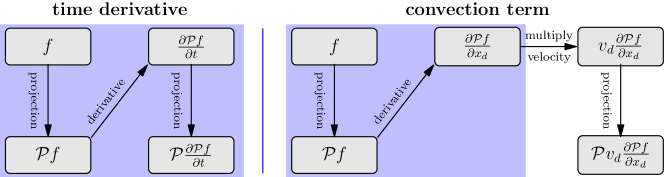
(a) Grad’s moment system

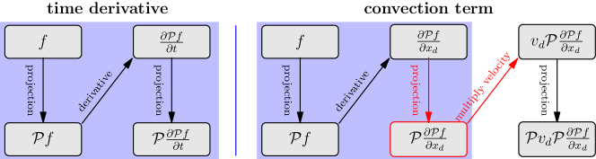
(b) Hyperbolic regularized moment system

Figure 1. Diagram of the procedure of Grad’s and regularized moment system.

Furthermore, we can diagram the procedure to derive Grad’s moment system in Fig. 1a. It is noticed in [19] that the time derivative and the spatial derivative are treated differently in such a process, as a projection operator is applied directly to the time derivative, while for the spatial derivative, this projection operator appears only after the velocity $v$ is multiplied. This difference causes the loss of hyperbolicity. By such observation, we have drawn a key conclusion in [19] that one should add a projection operator right in front of the spatial derivative to regain hyperbolicity, as is illustrated in Fig. 1b. The corresponding moment system is

(8) $${\mathcal{P}}\dfrac{\partial{{\mathcal{P}}f}}{\partial{t}}+\sum_{d=1}^{D}{\mathcal{P}}v_{d}{\color[rgb]{1,0,0}{\mathcal{P}}}\dfrac{\partial{{\mathcal{P}}f}}{\partial{x_{d}}}={\mathcal{P}}Q({\mathcal{P}}f),$$

where the additional projection operator is labeled in red. Using (5), one can claim that there exist the square matrices ${\bf M}_{d}$, $d=1,\dots,D$ such that

(9) $${\mathcal{P}}v_{d}{\mathcal{P}}\dfrac{\partial{{\mathcal{P}}f}}{\partial{x_{d}}}=\boldsymbol{{\mathcal{H}}}^{T}{\bf M}_{d}{\bf D}\dfrac{\partial{\boldsymbol{w}}}{\partial{x_{d}}},$$

and obtain the vector form of the regularized moment system as

(10) $${\bf D}\dfrac{\partial{\boldsymbol{w}}}{\partial{t}}+\sum_{d=1}^{D}{\bf M}_{d}{\bf D}\dfrac{\partial{\boldsymbol{w}}}{\partial{x_{d}}}=\boldsymbol{Q}.$$

Similar to (7), we have one more correspondence:

(11) $${\bf M}_{d}\leftrightarrow{\mathcal{P}}v_{d},$$

that is to say, the matrices ${\bf M}_{d}$ are the representation of the operators ${\mathcal{P}}v_{d}$ on $\mathbb{H}_{M}$. It is not difficult to check that the matrices ${\bf M}_{d}$ are symmetric due to the orthonormality of the basis ${\mathcal{H}}_{\alpha}$, so that any linear combination of the matrices ${\bf M}_{d}$ is real diagonalizable. One can also check the matrix ${\bf D}$ is invertible. Hence ${\bf D}^{-1}{\bf M}_{d}{\bf D}$ is similar to ${\bf M}_{d}$ so that the system (10) is globally hyperbolic. Moreover, if one multiplies ${\bf D}^{T}$ on both sides of (10), the resulting system

(12) $${\bf D}^{T}{\bf D}\dfrac{\partial{\boldsymbol{w}}}{\partial{t}}+\sum_{d=1}^{D}{\bf D}^{T}{\bf M}_{d}{\bf D}\dfrac{\partial{\boldsymbol{w}}}{\partial{x_{d}}}={\bf D}^{T}\boldsymbol{Q}$$

turns out to be a symmetric hyperbolic system of balance laws.

2.2. Hyperbolic regularization framework

Till now, the hyperbolicity of (10) has been proved using the Condition 3. Looking back on the whole procedure, one can find that the key point of the hyperbolic regularization is the extra projection operator in front of the spatial differentiation operator in (8). Meanwhile, the underlying mechanism to obtain hyperbolicity can be extended to much more general cases. For example, the radiative transfer equation has the form

$$\dfrac{\partial{f(t,\boldsymbol{x},\theta,\varphi)}}{\partial{t}}+\boldsymbol{\xi}(\theta,\varphi)\cdot\nabla_{\boldsymbol{x}}f(t,\boldsymbol{x},\theta,\varphi)=Q(f)(t,\boldsymbol{x},\theta,\varphi),\\ \boldsymbol{x}\in\mathbb{R}^{3},\quad\theta\in[0,\pi),\quad\varphi\in[0,2\pi),$$

where the velocity is given by $\boldsymbol{\xi}(\theta,\varphi)=(\sin\theta\cos\varphi,\sin\theta\sin\varphi,\cos\theta)^{T}$. To derive reduced models, one can replace the local equilibrium $f_{eq}$ in (2) by a nonnegative weight function $\omega$, and correspondingly, the orthogonal polynomials $\mathit{He}_{\alpha}$ should be replaced by the orthogonal basis functions $\phi_{\alpha}$ for the $L^{2}$ space weighted by $\omega$, so that the basis functions ${\mathcal{H}}_{\alpha}$ become $\Phi_{\alpha}:=\omega\phi_{\alpha}$. By letting $\mathbb{H}_{M}:=\mathrm{span}\{\Phi_{\alpha}:|\alpha|\leq M\}$, one can similarly define the projection operator ${\mathcal{P}}$ as in (3). As an extension of the globally hyperbolic moment system, we obtain

(13) $${\mathcal{P}}\dfrac{\partial{{\mathcal{P}}f}}{\partial{t}}+\sum_{d=1}^{D}{\mathcal{P}}\xi_{d}(\theta,\varphi){\mathcal{P}}\dfrac{\partial{{\mathcal{P}}f}}{\partial{x_{d}}}={\mathcal{P}}Q({\mathcal{P}}f).$$

Again, if the corresponding matrix ${\bf D}$ as in (6) is invertible, the resulting moment system is globally hyperbolic. We refer the readers to [6, 19, 21] for more details of such applications in radiative transfer equations.

This framework provides a concise and clear procedure to derive the hyperbolic moment system from a broad range of kinetic equations. It has been applied to many fields, including anisotropic hyperbolic moment system for Boltzmann equation [20], semiconductor device simulation [7], plasma simulation [11], density functional theory [8], quantum gas kinetic theory [16], and rarefied relativistic Boltzmann equation [32].

2.3. Further progress

The above framework provides an approach to handling the hyperbolicity of the moment system. However, the hyperbolicity is not the only concerned property. Preserving the hyperbolicity and other properties at the same time is often required in model reduction. Below we will list some recent attempts in this direction.

One of the interesting properties is to recover the asymptotic limits of the kinetic equations. For example, the first-order asymptotic hydrodynamic limit of the Boltzmann equation is the Navier-Stokes equations, and therefore it is desirable that the moment equations can preserve such a limit. For the classical Boltzmann equation, most moment systems can automatically preserve the Navier-Stokes limit if the stress tensor and heat flux are included. However, for the quantum Boltzmann equation, the equilibrium has a very special form, so that the moment system directly derived from the framework by taking the equilibrium as the weight function disobeys the Navier-Stokes limit [16]. In this case, the authors of [16] proposed a method called local linearization to regularize the moment system. Specifically, we assume the Grad-type system has the form as (6) and define $\hat{{\bf M}}_{d}(\boldsymbol{w})={\bf B}_{d}(\boldsymbol{w}){\bf D}(\boldsymbol{w})^{-1}$. In the regularization, the matrix $\hat{{\bf M}}_{d}(\boldsymbol{w})$ is replaced by ${\bf M}_{d}:=\hat{{\bf M}}_{d}(\boldsymbol{w}_{eq})$ with $\boldsymbol{w}_{eq}$ being the local equilibrium of the state $\boldsymbol{w}$. Such a method allows us to acquire both the hyperbolicity and Navier-Stokes limit simultaneously. The symmetry of ${\bf M}$ is thereby lost so that one has to use Condition 1 to prove the hyperbolicity.

Another relevant work is the nonlinear moment system for radiative transfer equation in [22, 21]. In order to retain the diffusion limit (similar to the Navier-Stokes limit for the Boltzmann equation), the authors pointed out that the projection operators in (13) at different places do not have to be same and revised (13) to be

(14) $$\tilde{{\mathcal{P}}}\dfrac{\partial{{\mathcal{P}}f}}{\partial{t}}+\sum_{d=1}^{D}\tilde{{\mathcal{P}}}\xi_{d}(\theta,\varphi)\tilde{{\mathcal{P}}}\dfrac{\partial{{\mathcal{P}}f}}{\partial{x_{d}}}=\tilde{{\mathcal{P}}}Q({\mathcal{P}}f).$$

The operators ${\mathcal{P}}$ and $\tilde{{\mathcal{P}}}$ are orthogonal projections onto different subspaces of $\mathbb{H}$. By a careful choice of the subspace for the operator $\tilde{{\mathcal{P}}}$, the diffusion limit can be achieved, and meanwhile, the symmetry of ${\bf M}$ corresponding to that in (10) is preserved, leading again to global hyperbolicity. This generalization has broadened the application the hyperbolic regularization framework and also permits us to take more properties of the kinetic equations into account.

Besides the hyperbolicity for the convection term, one may also be interested in the wellposedness of the complete moment system including the collision term. One related property is Yong’s first stability condition [38], which includes the constraints on the convection term, collision term, and the coupling of both. This stability condition is shown to be critical for the existence of the solutions in [37]. In [17], the authors have studied multiple Grad-type moment systems and confirmed that all of these systems satisfy Yong’s first stability condition.

Under this concise and flexible framework, one may wonder what is sacrificed for the hyperbolicity. By writing out the equations, one can immediately observe that the form of balance law is ruined by the hyperbolic regularization. A natural question is: how to define the discontinuity in the solution? More generally, one may ask: what is the effect of such a regularization on the accuracy of the model? In the following section, we will provide some clues using numerical experiments.

3. Numerical Validation

The application of the framework in the gas kinetic theory has been investigated in a number of works [3, 9, 10, 12], where many one- and two-dimensional examples have been numerically studied to show the validity of hyperbolic moment equations. However, these globally hyperbolic models, as an improvement of Grad’s original models, have never been compared with Grad’s models in terms of the modeling accuracy. The only direct comparison seen in the literature is in [10], wherein for a shock tube problem with a density ratio of $7.0$, the simulation of Grad’s moment equations breaks down and the corresponding hyperbolic moment equations appear to be stable. Without running numerical tests for the same problem for which both models work and comparing the results, it could be questioned whether we lose accuracy when fixing the hyperbolicity. Such doubt may arise since the globally hyperbolic models can be considered as a partial linearization of Grad’s models about the local Maxwellians.

In this section, we will make such straightforward comparison using the same numerical examples for both methods. For simplicity, we only consider the one-dimensional physics, for which both $x$ and $v$ are scalars. In this case, the characteristic polynomial for the Jacobian of the flux function has an explicit formula [3], so that the hyperbolicity of Grad’s equation can be easily checked. The underlying kinetic equation used in our test is the Boltzmann-BGK equation with a constant relaxation time

(15) $$\frac{\partial f}{\partial t}+v\frac{\partial f}{\partial x}=\frac{1}{\mathit{Kn}}(f_{eq}-f).$$

The ansatz of the distribution function is given by (3), so that (4) stands for Grad’s moment system, and (8) stands for the hyperbolic moment system. Below we are going to use two benchmark tests to show the performance of both types of models. In general, both Grad’s moment equations and the hyperbolic moment equations are solved by the first-order finite volume method with local Lax-Friedrichs numerical flux. Time splitting is applied to solve the advection part and the collision part separately, and for each part, the forward Euler method is applied. The CFL condition is utilized to determine the time step, and the Courant number is chosen as $0.9$. For Grad’s moment method, the maximum characteristic speed is obtained by solving the roots of the characteristic polynomial of the Jacobian, and the explicit expression of the charateristic polynomial has been given in [3]. For the hyperbolic moment method, the maximum characteristic speeds have been computed in [3]. The explicit form of the hyperbolic moment system (given in [3]) shows that its last equation contains a non-conservative product, which is discretized by central difference. In all the numerical examples, the number of grid cells is $1000$ if not otherwise specified. We have done the convergence test showing that for smooth solutions, such a resolution can provide solutions sufficiently close to the solutions on a much finer grid, so that their difference is invisible to the naked eye. When exhibiting the numerical results, we will mainly focus on the equilibrium variables including density $\rho$, velocity $u$, and temperature $\theta$, which are defined by

$$\rho(t,x) =\int_{\mathbb{R}}f(t,x,v)\,\mathrm{d}v,$$

$$u(t,x) =\frac{1}{\rho(t,x)}\int_{\mathbb{R}}vf(t,x,v)\,\mathrm{d}v,$$

$$\theta(t,x) =\frac{1}{\rho(t,x)}\int_{\mathbb{R}}[v-u(t,x)]^{2}f(t,x,v)\,\mathrm{d}v.$$

3.1. Shock structure

The structure of plane shock waves is frequently used as a benchmark test in the gas kinetic theory. It shows that the physical shock, which appears to be a discontinuity in the Euler equations, is actually a smooth transition from one state to another. The computational domain is $(-\infty,+\infty)$ so that no boundary condition is involved, and the initial data are

(16) $$f(0,x,v)=\left\{\begin{array}[]{ll}\dfrac{\rho_{l}}{\sqrt{2\pi\theta_{l}}}\exp\left(-\dfrac{(v-u_{l})^{2}}{2\theta_{l}}\right),&\text{if }x<0,\\[10.0pt] \dfrac{\rho_{r}}{\sqrt{2\pi\theta_{r}}}\exp\left(-\dfrac{(v-u_{r})^{2}}{2\theta_{r}}\right),&\text{if }x>0,\end{array}\right.$$

where all the equilibrium variables are determined by the Mach number $\mathit{Ma}$:

$$\rho_{l}=1,\qquad u_{l}=\sqrt{3}Ma,\qquad\theta_{l}=1,$$

$$\rho_{r}=\frac{2\mathit{Ma}^{2}}{\mathit{Ma}^{2}+1},\qquad u_{r}=\frac{\sqrt{3}\mathit{Ma}}{\rho_{r}},\qquad\theta_{r}=\frac{3\mathit{Ma}^{2}-1}{2\rho_{r}}.$$

We are interested in the steady-state of this problem. Since the parameter $\mathit{Kn}$ only introduces a uniform spatial scaling, it does not affect the shock structure. Therefore we simply set it to be $1$. Numerically, we set the computational domain to be $[-30,30]$. The boundary condition is provided by the ghost-cell method, and the distribution functions on the ghost cells are set to be the two states defined in (16).

3.1.1. Case 1: $\mathit{Ma}=1.4$ and $M=4$

In this case, both Grad’s system and the hyperbolic moment system work due to the relatively small Mach number. The numerical results are shown in Figure 2. By convention, we plot the normalized density, velocity, and temperature defined by

$$\bar{\rho}(x)=\frac{\rho(x)-\rho_{l}}{\rho_{r}-\rho_{l}},\quad\bar{u}(x)=\frac{u(x)-u_{r}}{u_{l}-u_{r}},\quad\bar{\theta}(x)=\frac{\theta(x)-\theta_{l}}{\theta_{r}-\theta_{l}},$$

so that the value of all variables are generally within the range $[0,1]$, unless the temperature overshoot is observed.

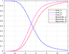
(a) Grad vs HME

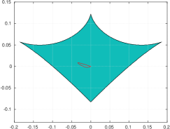
(b) Phase diagram of Grad’s solution

Figure 2. Left: The comparison of shock structures of two solutions with Mach number $1.4$ and $M=4$. Right: The green area is the hyperbolicity region (horizontal axis: $\hat{f}_{M-1}$, vertical axis: $\hat{f}_{M}$), and the red loop is the parametric curve $(\hat{f}_{M-1},\hat{f}_{M})$ with parameter $x$.

Figure 2b shows the hyperbolicity region of Grad’s moment equations. It has been proven in [3] that for the one-dimensional physics, the hyperbolicity region can be characterized by the following two dimensionless quantities:

$$\hat{f}_{M-1}=\frac{f_{M-1}}{\rho\theta^{(M-1)/2}},\qquad\hat{f}_{M}=\frac{f_{M}}{\rho\theta^{M/2}},$$

where $f_{M}$ and $f_{M-1}$ are the last two coefficients in the expansion (3). The red curve in Figure 2b provides the trajectory of Grad’s solution in this diagram. It can be seen that for such a small Mach number, the whole solution is well inside the hyperbolicity region, so that the simulation of Grad’s moment equations is stable. Figure 2a shows that both methods provide smooth shock structures, and the predictions for all the equilibrium variables are similar. This example confirms the applicability of both systems in weakly non-equilibrium regimes. Note that for one-dimensional physics, Grad’s equations do not suffer form the loss of hyperbolicity near equilibrium.

3.1.2. Case 2: $\mathit{Ma}=2.0$ and $M=4$

Now we increase the Mach number to introduce stronger non-equilibrium. The same plots are provided in Figure 3. In this example, despite the numerical diffusion, discontinuities can be identified without difficulty from the numerical solutions. These discontinuities, also known as subshocks, appear due to the insufficient characteristic speed in front of the shock wave, meaning that both systems are insufficient to describe the physics. To capture these discontinuities, $8000$ grid cells are used in the spatial discretization. This example shows significantly different shock structures predicted by both methods. For Grad’s moment equations, the subshock locates near $x=-7$, while for hyperbolic moment equations, the subshock appears near $x=-5$. The wave structures also differ a lot. By focusing on the high-density region, we find that the solution of hyperbolic moment equations is smoother, showing the possibly better description of the physics.

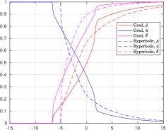
(a) Grad vs HME

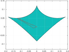
(b) Phase diagram of Grad’s solution

Figure 3. Left: The comparison of shock structures of two solutions with Mach number $2.0$ and $M=4$. Right: The green area is the hyperbolicity region (horizontal axis: $\hat{f}_{M-1}$, vertical axis: $\hat{f}_{M}$), and the red loop is the parametric curve $(\hat{f}_{M-1},\hat{f}_{M})$ with parameter $x$.

Here we remind the readers that the wave structure of hyperbolic moment equations may depend on the numerical method, due to its non-conservative nature. The locations and the strengths of the subshock may change when using the different shock conditions. However, we would like to argue that it is meaningless to justify any solution with subshocks for the hyperbolic moment equations, for it is unphysical and should not appear in the solution of the Boltzmann equation. In practice, the appearance of discontinuous solutions is an indication of the inadequate truncation of series, which inspires us to increase $M$ to get more reliable solutions without subshocks.

Figure 3b shows that Grad’s solution still locates within the hyperbolicity region, although the curve is already quite close to the boundary of the region. This example shows that even in its hyperbolicity region, Grad’s moment method may lose its validity.

3.1.3. Case 3: $\mathit{Ma}=2.0$ and $M=6$

Now we try to increase $M$ and carry out the simulation again for Mach number $2.0$. The results are given in Figure 4. With the hope that a larger $M$ can provide a better solution, we actually see that Grad’s moment equations lead to computational failure. The numerical solution before the computation breaks down is plotted in Figure 4a. Figure 4b clearly shows that this is caused by the loss of hyperbolicity. We believe that this implies the non-existence of the solution.

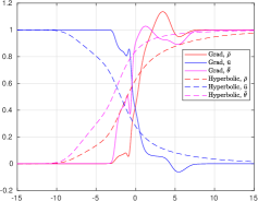
(a) Grad vs HME

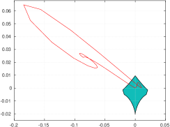
(b) Phase diagram of Grad’s solution

Figure 4. Left: The shock structure of hyperbolic moment equations for Mach number $2.0$ and $M=6$, and Grad’s solution before computational failure ($t=1.0$). Right: The green area is the hyperbolicity region (horizontal axis: $\hat{f}_{M-1}$, vertical axis: $\hat{f}_{M}$), and the red loop is the parametric curve $(\hat{f}_{M-1},\hat{f}_{M})$ with parameter $x$.

On the contrary, the simulation of hyperbolic moment equations is still stable. As expected, it provides a smooth shock structure and improves the result predicted by $M=4$.

3.1.4. Case 4: $\mathit{Ma}=1.7$ and $M=6$

In this example, we decrease the Mach number so that the shock structure of Grad’s equations can be found. Figure 5a shows that the results of both systems generally agree with each other, but it can be observed that hyperbolic moment equations provide smoother solutions than Grad’s system, so that it is likely to be more accurate. Therefore, despite the higher nonlinearity of Grad’s system, it does not necessarily help provide better solutions.

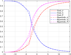
(a) Grad vs HME

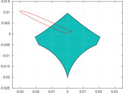
(b) Phase diagram of Grad’s solution

Figure 5. Left: The comparison of shock structures of two solutions with Mach number $1.7$ and $M=6$. Right: The green area is the hyperbolicity region (horizontal axis: $\hat{f}_{M-1}$, vertical axis: $\hat{f}_{M}$), and the red loop is the parametric curve $(\hat{f}_{M-1},\hat{f}_{M})$ with parameter $x$.

Interestingly, when looking at the phase diagram plotted in Figure 5b, we see that Grad’s solution has run out of the hyperbolicity region. It is to be further studied why the solution is still stable. Here we would like to conjecture that the collision term and the numerical diffusion help stabilize the numerical solution in the evolutionary process, and for the steady-state equations, solutions for non-hyperbolic equations may still exist. Nevertheless, all the above numerical tests show the superiority of hyperbolic moment equations for both accuracy and stability.

3.1.5. Case 5: $\mathit{Ma}=2.0$ and $M=10$

In this example, we would like to show the failure of both systems for a larger $M$. In Figure 6, we plot the results at $t=0.8$, where both numerical solutions contain negative temperatures. In [28], the reason for such a phenomenon has been explained, which lies in the divergence of the approximation (3) as $M$ tends to infinity. It is rigorously shown in [13] that when $\theta_{r}>2\theta_{l}$, for the solution of the steady-state BGK equation, the limit of ${\mathcal{P}}f$ (see (3)) as $M\rightarrow\infty$ does not exist. Here for $\mathit{Ma}=2.0$, the temperature behind the shock wave is $\theta_{r}=55/16>2=2\theta_{l}$. Thus for a large $M$, the divergence leads to a poor approximation of the distribution function, and it is reflected as a negative temperature in the numerical results. Such a divergence issue is independent of the subshock and the hyperbolicity, and should be regarded as a defect for both systems. The work on fixing the issue is ongoing.

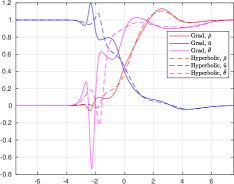
Figure 6. The numerical solution at $t=0.8$ for Mach number $2.0$ and $M=10$.

3.2. Fourier flow

In this test, we are interested in the performance of both methods with wall boundary conditions. The fluid we are concerned about is between two fully diffusive walls locating at $x=-1/2$ and $x=1/2$. For the Boltzmann-BGK equation (15), the boundary condition is

$$f(t,-1/2,v) =\frac{\rho_{l}}{\sqrt{2\pi\theta_{l}}}\exp\left(-\frac{v^{2}}{2\theta_{l}}\right),\qquad v>0,$$

$$f(t,1/2,v) =\frac{\rho_{r}}{\sqrt{2\pi\theta_{r}}}\exp\left(-\frac{v^{2}}{2\theta_{r}}\right),\qquad v<0,$$

where $\theta_{l,r}$ stands for the temperature of the walls, and $\rho_{l,r}$ is chosen such that

$$\int_{\mathbb{R}}vf(t,\pm 1/2,v)\,\mathrm{d}v=0.$$

Following [24], the boundary conditions of moment equations can be derived by taking odd moments of the diffusive boundary condition. We choose the initial condition as

(17) $$f(0,x,v)=\frac{1}{\sqrt{2\pi}}\exp\left(-\frac{v^{2}}{2}\right)$$

for all $x$. Again we are concerned only about the steady-state of the solution.

In our numerical experiments, we choose $\mathit{Kn}=0.3$, $\theta_{l}=1$ and $M=11$. Two test cases with $\theta_{r}=1.9$ and $\theta_{r}=2.7$ are considered. For the smaller temperature ratio $\theta_{r}=1.9$, the numerical results are given in Figure 7, where two solutions mostly agree with each other. The reference solution, computed using the discrete velocity model, is also provided in Figure 7a. It can be seen that both models provide reasonable approximations to the reference solution. The good behavior of Grad’s solutions can also be predicted by the phase diagram in Figure 7b, from which one can observe that the whole solution locates in the central area of the hyperbolicity region.

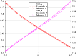
(a) Grad vs HME

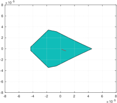
(b) Phase diagram of Grad’s solution

Figure 7. Left: Steady Fourier flow for $\theta_{r}=1.9$ (left vertical axis: $\rho$, right vertical axis: $\theta$). Right: The green area is the hyperbolicity region (horizontal axis: $\hat{f}_{M-1}$, vertical axis: $\hat{f}_{M}$), and the red line is the parametric curve $(\hat{f}_{M-1},\hat{f}_{M})$ with parameter $x$.

For $\theta_{r}=2.7$, the results are plotted in Figure 8. In this case, if we start the simulation of Grad’s equations from the initial data (17), the computation will break down due to the loss of hyperbolicity in the evolutional process. Therefore, we first run the simulation for hyperbolic moment equations from the initial data (17) and evolve the solution to the steady-state. Afterward, this steady-state solution serves as the initial data of Grad’s equations. Although the steady-state solution of Grad’s equations can be found using this technique, the approximation looks poorer than hyperbolic moment equations. The phase diagram (Figure 8b) shows that the solution near the left wall is outside the hyperbolicity region, so that the validity of boundary conditions on the left wall becomes unclear. In contrast, the hyperbolic moment equations still provide reliable approximation despite the high temperature ratio.

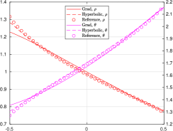
(a) Grad vs HME

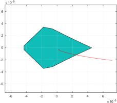
(b) Phase diagram of Grad’s solution

Figure 8. Left: Steady Fourier flow for $\theta_{r}=2.7$ (left vertical axis: $\rho$, right vertical axis: $\theta$). Right: The green area is the hyperbolicity region (horizontal axis: $\hat{f}_{M-1}$, vertical axis: $\hat{f}_{M}$), and the red line is the parametric curve $(\hat{f}_{M-1},\hat{f}_{M})$ with parameter $x$.

3.3. A summary of numerical experiments

In all the above numerical experiments, we see that despite the loss of some nonlinearity, the hyperbolicity fix does not appear to lose accuracy in any of the numerical tests. In regimes with moderate non-equilibrium effects, Grad’s equations may provide solutions outside the hyperbolicity region without numerical instability. In this situation, our experiments show that the hyperbolicity fix is likely to improve the accuracy of the model. It has also been demonstrated that other issues, such as subshocks and divergence, are not related to the hyperbolicity, and these issues have to be addressed independently.

4. Conclusion

The loss of hyperbolicity, as one of the major obstacles for the model reduction in gas kinetic theory, is almost cleared through the research works in recent years. With a handy framework introduced in Section 2, we can safely move our focus of model reduction to other properties such as the asymptotic limit, the stability, and the convergence issues. Our numerical experiments show that the hyperbolic regularization does not harm the accuracy of the model. It is our hope that such a framework can inspire more thoughts in the development of dimensionality reduction even beyond the kinetic theory.

References

- [1] L. Boltzmann. Weitere studien über das wärmegleichgewicht unter gas-molekülen. Wiener Berichte, 66:275–370, 1872.
- [2] Yves Bourgault, Damien Broizat, and Pierre-Emmanuel Jabin. Convergence rate for the method of moments with linear closure relations. Kinetic and Related Models, 8(1):1–27, 2015.
- [3] Z. Cai, Y. Fan, and R. Li. Globally hyperbolic regularization of Grad’s moment system in one dimensional space. Comm. Math. Sci., 11(2):547–571, 2013.
- [4] Z. Cai, Y. Fan, and R. Li. Globally hyperbolic regularization of Grad’s moment system. Comm. Pure Appl. Math., 67(3):464–518, 2014.
- [5] Z. Cai, Y. Fan, and R. Li. On hyperbolicity of 13-moment system. Kinet. Relat. Mod., 7(3):415–432, 2014.
- [6] Z. Cai, Y. Fan, and R. Li. A framework on moment model reduction for kinetic equation. SIAM J. Appl. Math., 75(5):2001–2023, 2015.
- [7] Z. Cai, Y. Fan, R. Li, T. Lu, and Y. Wang. Quantum hydrodynamic model by moment closure of wigner equation. J. Math. Phys., 53(10):103503, 2012.
- [8] Z. Cai, Y. Fan, R. Li, T. Lu, and W. Yao. Quantum hydrodynamic model of density functional theory. Journal of Mathematical Chemistry, 51(7):1747–1771, 2013.
- [9] Z. Cai, Y. Fan, R. Li, and Z. Qiao. Dimension-reduced hyperbolic moment method for the Boltzmann equation with BGK-type collision. Commun. Comput. Phys., 15(5):1368–1406, 2014.
- [10] Z. Cai, R. Li, and Z. Qiao. Globally hyperbolic regularized moment method with applications to microflow simulation. Computers and Fluids, 81:95–109, 2013.
- [11] Z. Cai, R. Li, and Y. Wang. Solving Vlasov equation using NR method. SIAM J. Sci. Comput., 35(6):A2807–A2831, 2013.
- [12] Z. Cai and M. Torrilhon. Numerical simulation of microflows using moment methods with linearized collision operator. J. Sci. Comput., 74(1):336–374, 2018.
- [13] Z. Cai and M. Torrilhon. On the Holway-Weiss debate: Convergence of the Grad-moment-expansion in kinetic gas theory. Phys. Fluids, 31:126105, 2019.
- [14] C. Cercignani. Mathematical Methods in Kinetic Theory. Springer US, New York, 1969.
- [15] S. Chapman. On the law of distribution of molecular velocities, and on the theory of viscosity and thermal conduction, in a non-uniform simple monatomic gas. Phil. Trans. R. Soc. A, 216(538–548):279–348, 1916.
- [16] Y. Di, Y. Fan, and R. Li. 13-moment system with global hyperbolicity for quantum gas. Journal of Statistical Physics, 167(5):1280–1302, 2017.
- [17] Y. Di, Y. Fan, R. Li, and L. Zheng. Linear stability of hyperbolic moment models for Boltzmann equation. Numerical Mathematics: Theory, Method and Application, 2016.
- [18] D. Enskog. The numerical calculation of phenomena in fairly dense gases. Arkiv Mat. Astr. Fys., 16(1):1–60, 1921.
- [19] Y. Fan, J. Koellermeier, J. Li, R. Li, and M. Torrilhon. Model reduction of kinetic equations by operator projection. Journal of Statistical Physics, 162(2):457–486, 2016.
- [20] Y. Fan and R. Li. Globally hyperbolic moment system by generalized Hermite expansion. Scientia Sinica Mathematica, 45(10):1635–1676, 2015.
- [21] Yuwei Fan, Ruo Li, and Lingchao Zheng. A nonlinear hyperbolic model for radiative transfer equation in slab geometry. arXiv preprint arXiv:1911.05472, 2019.
- [22] Yuwei Fan, Ruo Li, and Lingchao Zheng. A nonlinear moment model for radiative transfer equation in slab geometry. Journal of Computational Physics, 404:109128, 2020.
- [23] Tamas I. Gombosi. Gaskinetic Theory. Cambridge University Press, 1994.
- [24] H. Grad. On the kinetic theory of rarefied gases. Comm. Pure Appl. Math., 2(4):331–407, 1949.
- [25] H. Grad. The profile of a steady plane shock wave. Comm. Pure Appl. Math., 5(3):257–300, 1952.
- [26] H. Grad. Principles of the kinetic theory of gases. Handbuch der Physik, 12:205–294, 1958.
- [27] Stewart Harris. An introduction to the theory of the Boltzmann equation. Holt, Rinehart and Winston, Inc., 1971.
- [28] L. H. Holway. Existence of kinetic theory solutions to the shock structure problem. Phys. Fluids, 7(6):911–913, 1965.
- [29] James H. Jeans. An Introduction to The Kinetic Theory of Gases. Cambridge University Press, 1967.
- [30] M. Junk. Domain of definition of Levermore’s five-moment system. J. Stat. Phys., 93(5):1143–1167, 1998.
- [31] J. Koellermeier, R. Schaerer, and M. Torrilhon. A framework for hyperbolic approximation of kinetic equations using quadrature-based projection methods. Kinet. Relat. Mod., 7(3):531–549, 2014.
- [32] Yangyu Kuang and Huazhong Tang. Globally hyperbolic moment model of arbitrary order for one-dimensional special relativistic Boltzmann equation. Journal of Statistical Physics, 167(5):1303–1353, 2017.
- [33] C. D. Levermore. Moment closure hierarchies for kinetic theories. J. Stat. Phys., 83(5–6):1021–1065, 1996.
- [34] J. McDonald and M. Torrilhon. Affordable robust moment closures for CFD based on the maximum-entropy hierarchy. J. Comput. Phys., 251:500–523, 2013.
- [35] I. Müller and T. Ruggeri. Extended Thermodynamics, volume 37 of Springer tracts in natural philosophy. Springer-Verlag, New York, 1993.
- [36] I. Müller and T. Ruggeri. Rational Extended Thermodynamics, Second Edition, volume 37 of Springer tracts in natural philosophy. Springer-Verlag, New York, 1998.
- [37] Y. Peng and V. Wasiolek. Uniform global existence and parabolic limit for partially dissipative hyperbolic systems. Journal of Differential Equations, 2016.
- [38] W.-A. Yong. Singular perturbations of first-order hyperbolic systems with stiff source terms. Journal of differential equations, 155(1):89–132, 1999.
- [39] Weifeng Zhao, Wenan Yong, and Lishi Luo. Stability analysis of a class of globally hyperbolic moment system. Communications in Mathematical Sciences, 15(3):609–633, 2016.