Extreme quasars as distance indicators in cosmology

Abstract

Quasars accreting matter at very high rates (known as extreme Population A [xA] quasars, possibly associated with super-Eddington accreting massive black holes) may provide a new class of distance indicators covering cosmic epochs from present day up to less than 1 Gyr from the Big Bang. At a more fundamental level, xA quasars are of special interest in studies of the physics of AGNs and host galaxy evolution. However, their observational properties are largely unknown. xA quasars can be identified in relatively large numbers from major optical surveys over a broad range of redshifts, and efficiently separated from other type-1 quasars thanks to selection criteria defined from the systematically-changing properties along the quasars main sequence. It has been possible to build a sample of $\sim$ 250 quasars at low and intermediate redshift, and larger samples can be easily selected from the latest data releases of the Sloan Digital Sky Survey. A large sample can clarify the main properties of xA quasars which are expected – unlike the general population of quasars – to radiate at an extreme, well defined Eddington ratio with small scatter. As a result of the small scatter in Eddington ratio shown by xA quasars, we propose a method to derive the main cosmological parameters based on redshift-independent “virial luminosity” estimates from measurements of emission line widths, roughly equivalent to the luminosity estimates based from line width in early and late type galaxies. A major issue related to the cosmological application of the xA quasar luminosity estimates from line widths is the identification of proper emission lines whose broadening is predominantly virial over a wide range of redshift and luminosity. We report on preliminary developments using the AlIII$\lambda$1860 intermediate ionization line and the Hydrogen Balmer line H$\beta$ as virial broadening estimators, and we briefly discuss the perspective of the method based on xA quasars.

1 Keywords:

quasar main sequence – line profiles – emission lines – supermassive black holes – black hole physics – dark energy – cosmological paremeters – cosmology

2 Introduction

Quasars show a rich spectrum of emission lines coming from a side range of ionic species (e.g., Netzer, 2013). Differences in line profiles, line shifts, line intensities hint at diversity in dynamical conditions and ionization levels of the broad line region (BLR; Sulentic et al. 2000). There is a general consensus that the H$\beta$ and low-ionization lines (LILs) in general are mainly broadened via Doppler effect from emitting gas virial motion, while high-ionization lines (HILs) are more affected by non-virial broadening, probably associated with a disk wind or clumpy outflows (e.g., Marziani et al., 1996; Proga et al., 2000; Elvis, 2000; Richards et al., 2011, for a variety of approaches). The relative prominence of the wind and disk component reflects the different balance between radiation and gravitation forces (Ferland et al., 2009; Marziani et al., 2010; Netzer and Marziani, 2010), and is systematically changing along the quasar main sequence (MS). If the main driver of the stellar H-R diagram can be considered mass, for the quasar main sequence it is the luminosity to black hole mass ratio that apparently matters most (Boroson and Green, 1992; Sulentic et al., 2000; Marziani et al., 2001; Shen and Ho, 2014; Sun and Shen, 2015; Panda et al., 2019). In addition, unlike stars, quasars are not endowed of spherical symmetry but only by axial symmetry: the spin of the black hole and the axis of the accretion disk define axes of symmetry and a preferential plane (i.e., the equatorial plane of the black hole, the inner accretion disk plane). Aspect becomes an important parameters for AGN. The effect is most noticeable in the distinction between type-1 and type-2 (obscured) AGN (e.g., Antonucci, 1993; Urry and Padovani, 1995), but is relevant also for type-1 AGN (unobscured), as the viewing angle (defined as the angle between the disk axis and the line of sight) may range between 0 and 60 degrees.

Quoting Marziani et al. (2001), we can say that …the observed correlation …can be accounted for if it is primarily driven by the ratio of AGN luminosity to black hole mass ($L/M\propto\,$ $L/L_{\mathrm{Edd}}$, Eddington ratio) convolved with source orientation. Several recent reviews papers have dealt with the quasar main sequence (e.g., Sulentic et al., 2008; Sulentic and Marziani, 2015; Marziani et al., 2018b). Here we will summarize briefly the basic concepts and trends (§3), afterward focusing on a particular class of objects, the strongest Feii emitters along the sequence (§4). The basis of the virial luminosity estimations are then presented in §5, also in an aspect-angle dependent form. Preliminary results for cosmology are illustrated in §6.

3 A main sequence for type-1 (unobscured) quasars

The Main Sequence stems from the definition of the so-called Eigenvector 1 of quasars by a Principal Component Analysis of PG quasars (Boroson and Green, 1992). The MS of quasars is customarily presented in an optical plane defined by the parameter of Feii prominence $R_{\mathrm{FeII}}$  (the intensity ratio between the FeII blend at $\lambda$4570 and H$\beta$) and by the full-width half maximum (FWHM) of H$\beta$ (Boroson and Green, 1992; Sulentic et al., 2000), and associated with the anti- correlation between strength of Feii$\lambda$4570 (or [Oiii]$\lambda$5007 peak intensity) and width of H$\beta$. Feii  maintains the same relative intensity of the emission blends (at least to a first approximation) but Feii intensity with respect to H$\beta$ changes from object to objects, and in the strongest Feii emitters, Feii  emission can dominate the thermal balance of the BLR (Marinello et al., 2016). Therefore it does not appear surprising that the Feii dominance parameters is a fundamental parameter in organising the diversity of type-1 quasars. The FWHM H$\beta$ is related to the velocity field in the low-ionisation part of the BLR, and ultimately associated with the orientation angle, black hole mass and Eddington ratio (§3.2). Since 1992, the Eigenvector 1 MS has been found in increasingly larger samples, involving more and more extended sets of multifrequency parameters (Sulentic et al., 2007; Zamfir et al., 2010; Shen and Ho, 2014; Wolf et al., 2019). In addition to the parameters defining the optical plane, $R_{\mathrm{FeII}}$ and FWHM(H$\beta$), several multifrequency parameters related to the accretion process and the accompanying outflows are also correlated (see Fraix-Burnet et al., 2017, for an exhaustive list).

The MS allows for the definition of spectral types (Sulentic et al., 2002; Shen and Ho, 2014). In addition Sulentic et al. (2000) introduced a break at 4000 km s^-1 and the distinction between Population A (FWHM H$\beta$$\lesssim$4000 km s^-1) which includes the Narrow Line Seyfert 1 (NLSy1s), and Population B of broader sources. Extreme Population A (xA) sources are the ones toward the high $R_{\mathrm{FeII}}$ end of the main sequence ($R_{\mathrm{FeII}}$$>$ 1). The optical spectra of the prototypical Narrow Line Seyfert 1 (NLSy1) I Zw 1 and the Seyfert-1 nucleus NGC 5548 illustrate the changes that occur along the sequence. I Zw 1 (a prototypical xA source) shows a low-ionization appearance, with strong Feii, weak [Oiii]$\lambda\lambda$4959,5007, and a spiky H$\beta$ broad profile; on the converse the optical spectrum of NGC 5548 suggests a higher degree of ionization, with low Feii emission, strong [Oiii]$\lambda\lambda$4959,5007. It is expedient to consider the Hydrogen Balmer line H$\beta$ and the Civ$\lambda$1549 as prototypical optical and UV LILs and HILs, respectively. Comparing the Civ$\lambda$1549 and H$\beta$ lines yields important information: in the spectra of NGC 5548 the two lines show similar profile, while in the ones of I Zw 1 the Civ$\lambda$1549 emission is almost fully blue shifted with respect to a predominantly symmetric and unshifted (with respect to rest frame) H$\beta$ profile (e.g., Sulentic et al., 2000; Leighly, 2004; Coatman et al., 2016).

The comparison between LILs and HILs has provided insightful constraints of the BLR at low-$z$ (Marziani et al., 1996), and this is even more true if the comparison of H$\beta$ and Civ$\lambda$1549 is carried out at high $L$  (Sulentic et al., 2017; Bisogni et al., 2017; Shen, 2016; Vietri et al., 2018). Perhaps the most remarkable fact is that a LIL-BLR appears to remain basically virialized (Marziani et al., 2009; Sulentic et al., 2017). The Civ$\lambda$1549 blueshift depends on luminosity (the median $c(\frac{1}{2})$ is $\approx$ 2600 km s^-1 and 1800 km s^-1 for Pop. A and B radio-quiet (RQ) at high-$L$ against less than 1000 km s^-1at low-$L$), but the dependence is not strong, and can be accounted for in the framework of a radiation driven winds. In spite of the extremely high amplitude Civ$\lambda$1549 blueshifts of Pop. A quasars at the highest luminosity $L\gtrsim 10^{47}$ erg s^-1, the H$\beta$ profile remains (almost) symmetric and unshifted with respect to rest frame. Fig. 1 shows the emission line profiles of H$\beta$, Civ$\lambda$1549, and Aliii$\lambda$1860 and Siiii]$\lambda$1892 in three quasars of widely different luminosity. LILs in the optical and UV remains symmetric and unshifted. The lines have been decomposed into two main components.

• The broad component (BC), also known as the intermediate component, the core component or the central broad component following various authors (e.g., Brotherton et al., 1994; Popović et al., 2002; Adhikari et al., 2016; Kovačević-Dojčinović and Popović, 2015). Following Sulentic et al. (2002), the BC is modeled by a symmetric and unshifted profile (Lorentzian for Pop. A or Gaussian for Pop. B), as it is believed to be associated with a virialized BLR subsystem. The virialized BLR could be defined as the BLR subregion that is in the condition to emit FeII. Given the stratification of ionization in the BLR, the Feii emission is apparently weighted toward outer radii with respect to H$\beta$  (Barth et al., 2013), as also supported by the slightly narrower Feii with respect to H$\beta$ (e.g., Sulentic et al., 2004). The regions emitting H$\beta$ BC and Feii are however believed to be largely co-spatial.

• The blue shifted component (BLUE). A strong blue excess in Pop. A Civ profiles is obvious, as in some Civ profiles – like the one of the xA prototype I Zw1 – BLUE dominates the total emission line flux (Marziani et al., 1996; Leighly and Moore, 2004). For BLUE, there is no evidence of a “stable” profile, and a “stable” profile is not expected, as we are dealing with a component that is likely subject to phenomena associated with turbulence and hydrodynamic instabilities. In our recent work (Sulentic et al., 2017), we have modeled the blueshifted excess adding to the symmetric BC profile one or more skew-normal distributions (Azzalini and Regoli, 2012). The “asymmetric Gaussian” fitting function is, at present, empirically motivated by the often-irregular BLUE profile in Civ and Mgii$\lambda$2800.

The line width of the LILs clearly increases with luminosity passing from $\sim 1000$ km s^-1 to 5000 km s^-1 from $\log L\sim$ 44 to $\sim 47$. This behaviour — typical of Pop. A quasars — suggests that a virialized sub-system emitting mainly LILs coexists with outflowing gas. Even at the highest luminosity the data (Sulentic et al., 2017; Vietri et al., 2018; Coatman et al., 2016) remain consistent with a scenario that posits a dichotomy within the BLR, where the blue shifted emission is produced in clumps of gas or a continuous wind (Collin-Souffrin et al., 1988; Elvis, 2000), and LILs are emitted by gas in virial motion. In this scenario, we observe a net blueshift in Civ$\lambda$1549 because of the large gas velocity field component along the radial direction, with the receding side of the flow obscured by an optically thick equatorial structure, most likely associated with the accretion disk. I Zw 1 fits very well this interpretation: if LILs are emitted in the flattened disk structure, the H$\beta$ should appear narrow, while Civ$\lambda$1549 emission broader and shifted to the blue, which is indeed the case (Marziani et al., 1996; Leighly, 2004).

3.1 The definition of spectral types

The data point occupation in the plane $R_{\mathrm{FeII}}$– FWHM(H$\beta$) allows for the definition of spectral NLSy1s types; A1, A2… in order of increasing $R_{\mathrm{FeII}}$; A1, B1, B1+ .…in order of increasing FWHM(H$\beta$). This has the considerable advantage that a composite over all spectra within each bin should be representative of objects in similar dynamical and physical conditions. In principle, a prototypical object can be defined for each spectral type to analyze systematic changes along the quasar MS. Before summarizing some basic trends, it is helpful to recall the main motivations behind the distinction between Population A and B.

3.2 Population A and NLSy1s

Why choose a FWHM limit for H$\beta$ at 4000 km s^-1? Many studies even in recent times distinguish between NLSy1s (FWHM H$\beta$ $\lesssim 2000$ km s^-1) and rest of type 1 AGNs (e.g., Cracco et al., 2016). The basic reason to extend the limit to 4000 km s^-1 is that several important properties of NLSy1s are not distinguishable from “the rest of Population A” in the range $2000$ km s^-1$\lesssim$ FWHM(H$\beta$) $\lesssim 4000$ km s^-1. NLSy1s are located at the low-end of the distribution of FWHM(H$\beta$) in the samples of Shen et al. (2011); Zamfir et al. (2010) without any apparent discontinuity. NLSy1s and the rest of Population A show no apparent discontinuity as far as line profiles are concerned (Cracco et al., 2016). Composite H$\beta$ profiles of spectral types along the MS are consistent with a Lorentzian as do the rest of Population A sources. A recent analysis of composite line profiles in narrow FWHM(H$\beta$) ranges ($\delta$ FWHM = 1000 km s^-1) confirms that there is no discontinuity at 2000 km s^-1; best fits of profiles remain Lorentzian up to at least 4000 km s^-1. A change in the H$\beta$ profile shape occurs around FWHM(H$\beta$) = 4000 km s^-1 at the Population A limit, not at the one of NLSy1s (Sulentic et al., 2002). No significant difference between CIV$\lambda$1549 centroids at half-maximum of NLSy1s and rest of Pop. A is detected using the HST/FOS data of the Sulentic et al. (2007) sample (Marziani et al., 2018a). In addition NLSy1s span a broad range of spectral types, the $R_{\mathrm{FeII}}$ parameter being between almost 0 and 2 in the quasi-totality of sources, as the rest of Population A sources do.

A complete tracing of the MS at high $L$ is still missing (we consider high-luminosity sources the quasars with bolometric $\log L\gtrsim 47$ [erg/s]): the H$\beta$ spectral range is accessible only with IR spectrometers, and high-luminosity quasars are exceedingly rare also at $z\lesssim 1$. The main effect of a systematic increase in black hole mass $M_{\mathrm{BH}}$ can be predicted. If the motion in the LIL-BLR is predominantly virial, we can write the central black hole mass $M_{\mathrm{BH}}$ as a virial mass :

$$M_{\rm BH}=\frac{r_{\mathrm{BLR}}\delta v_{\rm K}^{2}}{G}$$ (1)

which follows from the application of the virial theorem in case all gravitational potential is associated with a central mass. $\delta v_{\rm K}$ is the virial velocity module, $r_{\mathrm{BLR}}$ the radius of the BLR, $G$ the gravitational constant. Eq. 1 can be of use if we can relate $\delta v_{\rm K}$ to the observed velocity dispersion, represented here by the FWHM of the line profile:

$$M_{\rm BH}=f_{\rm S}\frac{r{\rm{}_{\mathrm{BLR}}FWHM}^{2}}{G}$$ (2)

via the structure factor (a.k.a. as form or virial factor) whose definition is given by:

$$\delta v_{\rm K}^{2}=f_{\rm S}{\rm FWHM}^{2}$$ (3)

If the BLR radius follows a scaling power-law with luminosity ($r\propto L^{\mathrm{a}}$, Kaspi et al. 2000; Bentz et al. 2013), then

$$\mathrm{FWHM}\propto f_{\mathrm{S}}^{-\frac{1}{2}}{L}^{\frac{1-a}{2}}\left(\frac{L}{M_{\mathrm{BH}}}\right)^{-\frac{1}{2}}$$ (4)

Or, equivalently,

$$\mathrm{FWHM}\propto f_{\mathrm{S}}^{-\frac{1}{2}}\left(\frac{L}{M_{\mathrm{BH}}}\right)^{-\frac{a}{2}}M_{\mathrm{BH}}^{\frac{1-a}{2}}.$$ (5)

If $a=0.5$, the FWHM grows with $M_{\mathrm{BH}}$^0.25, meaning a factor of 10 (!) for $\log L$ passing from 44 (relatively low luminosity) to 48 (very luminous) quasars. The trend may not be detectable in low-$z$ flux limited samples, but becomes appreciable if sources over a wide range in $L$ are considered. At high $M_{\mathrm{BH}}$, the MS becomes displaced toward higher FWHM values in the optical plane of the MS; the displacement most likely accounts for the wedge shaped appearance of the MS if large samples of SDSS quasars are considered (Shen and Ho, 2014).

If we consider a physical criterion for the distinction between Pop. A and B a limiting Eddington ratio ($\log$ $L/L_{\mathrm{Edd}}$$\sim$ 0.1 — 0.2), then the separation at fixed $L/L_{\mathrm{Edd}}$ becomes luminosity dependent. In addition FWHM(H$\beta$) is strongly sensitive to viewing angle, via the dependence on $\theta$ of the $f_{\mathrm{S}}$ (§5.2). An important consequence is that a strict FWHM limit has no clear physical meaning: its interpretation depends on sample properties. At low and moderate luminosity ($\log L\lesssim$ 47 [erg s^-1]), the limit at 4000 km s^-1 selects mainly sources with $\log$ $L/L_{\mathrm{Edd}}$$\gtrsim$ 0.1 — 0.2 i.e., above a threshold that is also expected to be relevant in terms of accretion disk structure. However, the selection is not rigorous, since a minority of low $L/L_{\mathrm{Edd}}$ sources observed pole-on (and hence with FWHM narrower because of a pure orientation effect) are expected to be below the threshold FWHM at 4000 km s^-1. Such sources include core-dominated radio-loud quasars whose viewing angle $\theta$ should be relatively small (Marziani et al., 2001; Zamfir et al., 2008). They are expected to be rare, because the probability of observing a source at a viewing angle $\theta$ is $P(\theta)\propto\sin\theta$, although their numbers is increased in flux-limited sample because of the Malmquist effect. As a conclusion, we can state that separating Pop. A and B at 4000 km s^-1  makes sense for low $z$ sample and that, by a fortunate circumstances, Pop. A includes the wide majority of relatively high $L/L_{\mathrm{Edd}}$ sources.

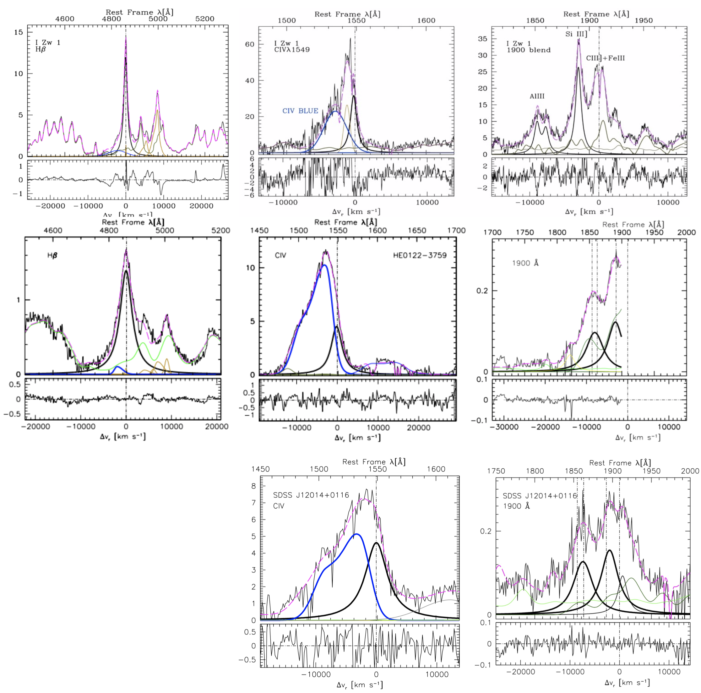
Figure 1: Intercomparison of line profiles of H$\beta$(left), Civ$\lambda$1549 (middle) and Aliii$\lambda$1860 in the 1900 blend for three xA quasars of widely different luminosity (top: I Zw 1 (Marziani et al., 2010); middle: HE0122-3759 (Sulentic et al., 2017); bottom: SDSS J12014-0116 (Negrete et al., 2012)). The thin black line shows the continuum subtracted spectra, the thick black lines trace the virialized symmetric broad component, and the thick blue line the blueshifted excess. Feii emission is shown in lemon green, and narrow lines in orange color. The magenta dot-dashed line traces the model of the spectrum including all emission components. Note the absence or weakness of the BLUE for both H$\beta$ and Aliii$\lambda$1860.

4 Extreme Population A: Selection and physical conditions

As mentioned in §2, Eddington ratio is a parameter that is probably behind the $R_{\mathrm{FeII}}$ sequence in the optical plane of the MS. It is still unclear why it is so. At a first glance, the low-ionisation appearance of sources whose Eddington ratio is expected to be higher is puzzling. Marziani et al. (2001) accounted for this results including several observational trends that could lower the ionisation parameter with increasing $R_{\mathrm{FeII}}$. More recent results include a careful assessment of the role of metallicity (Panda et al., 2018, 2019). There is empirical evidence of a correlation between $R_{\mathrm{FeII}}$ and $L/L_{\mathrm{Edd}}$, but the issue is compounded with the strong effect of orientation on the line broadening, and hence on $M_{\mathrm{BH}}$ and $L/L_{\mathrm{Edd}}$ computation. As an estimate of the viewing angle is not possible for individual radio-quiet sources (even if some recent works provide new perspectives), conventional $M_{\mathrm{BH}}$ (Eq. 1) and $L/L_{\mathrm{Edd}}$ estimates following the definitions in the previous section suffer of a large amplitude scatter (Marziani et al., 2019, and references therein). Mass estimates over a broad range of FWHM are especially uncertain, and may lead to sample-dependent, spurious trends. Even if a combination of effects related to Eddington ratio, viewing angle, and metal content reproduce the sequence, and accounts for the relative distribution of sources in each spectral bin, the actual structure of the BLR and its relation with the accretion mode is still unclear. This said, if our basic interpretation of $R_{\mathrm{FeII}}$ as mainly related to $L/L_{\mathrm{Edd}}$ is correct, then the strongest Feii emitters should be the highest radiators. For instance, Sun and Shen (2015) provide evidence not dependent on the viewing angle: in narrow bins of luminosity, the stellar velocity dispersion of the host spheroid (a proxy for $M_{\mathrm{BH}}$) is anti correlated with $R_{\mathrm{FeII}}$, implying that $L/L_{\mathrm{Edd}}$ increases with Feii. The fundamental plane of accreting black holes (Du et al., 2016) correlates $L/L_{\mathrm{Edd}}$ and dimensionless accretion rate with $R_{\mathrm{FeII}}$ and with the “Gaussianity” parameter $D=$FWHM/$\sigma$ of H$\beta$. Both methods imply that the highest $R_{\mathrm{FeII}}$ corresponds to the highest $L/L_{\mathrm{Edd}}$.

If we select spectral types along the sequence satisfying the condition $R_{\mathrm{FeII}}$$\gtrsim 1$ (A3, A4, …), we select spectra with distinctively strong Feii emission and Lorentzian Balmer line profiles. They account for $\sim$ 10% of quasars in low-z, optically selected sample FeII in Pop. A.

The simple selection criterion

• $R_{\mathrm{FeII}}$= FeII$\lambda$4570 blend/H$\beta$ $>$ 1.0

corresponds to the selection criterion:

• AlIII $\lambda$1860/SiIII]$\lambda$1892$>$0.5 & SiIII]$\lambda$1892/ CIII]$\lambda$1909$>$1

The $R_{\mathrm{FeII}}$$>$1 and the UV selection criteria are believed to be equivalent. Marziani and Sulentic (2014a) compared the distribution of sources satisfying $R_{\mathrm{FeII}}$$\gtrsim 1$ in the plane AlIII $\lambda$1860/SiIII]$\lambda$1892 vs SiIII]$\lambda$1892/ CIII]$\lambda$1909, and found that these sources were confined in a box satisfying the boundary conditions AlIII $\lambda$1860/SiIII]$\lambda$1892$>$0.5 & SiIII]$\lambda$1892/ CIII]$\lambda$1909$>$1, as expected if the two selection criteria are consistent. The number of sources for which this check could be carried out is however small, and xA sources are located in borderline positions. Work is in progress to test the consistency on a larger sample.

However, the UV xA spectrum is very easily recognizable, as shown by the composite spectrum of Martínez-Aldama et al. (2018). Lines have low equivalent width: some xAs are weak lined quasars (W(Civ$\lambda$1549) $\leq$ 10 Å, WLQ Diamond-Stanic et al., 2009), whereas WLQs can be considered as the extreme of extreme Pop. A. The Ciii$\lambda$1909 emission almost disappears. In the plane $\log U-\log n_{\mathrm{H}}$ defined by CLOUDY simulation, UV line intensity ratio converge toward extreme values for density (high, $n_{\mathrm{H}}>10^{12}-10^{13}$ cm³), ionization (low, ionization parameter $U\sim 10^{-3}-10^{-2.5}$). Extreme values of metallicity are also derived from the intensity ratios CIV/AlIII CIV/HeII AlIII/SiIII] (Negrete et al., 2012; Martínez-Aldama et al., 2018, Sniegowska et al. 2019 in preparation)), most likely above 20 times solar or with abundances anomalies that increase selectively aluminum or silicon, or both.

In addition to the selection criteria, a virial broadening estimator equivalent to H$\beta$ should be defined from the emission line in the rest frame UV spectrum. The Civ$\lambda$1549 line is unsuitable unless heavy corrections are applied (Coatman et al., 2017; Marziani et al., 2019). However, the UV spectrum of xA quasars at z $\sim 2$ show symmetric low-ionization and blueshifed high- ionization lines even at the highest luminosity (Martínez-Aldama et al., 2018, and reference therein). The results of a preliminary analysis is shown in Fig. 2: the FWHM of H$\beta$ and Aliii$\lambda$1860 for Pop. A objects are well correlated, with no systematic deviation from the 1:1 relation. Work is in progress to focus this systematic comparison to a sizeable sample of xA sources.

The Eddington ratio precise values depend on the normalization applied; the relevant result is that xA quasars radiate at extreme $L/L_{\mathrm{Edd}}$ along the MS with small dispersion (Marziani and Sulentic, 2014a). This results is consistent from the expectation of accretion disks at very large accretion rates. Accretion disk theory predicts low radiative efficiency at high accretion rate and that $L/L_{\mathrm{Edd}}$ saturates toward a limiting values (Mineshige et al., 2000; Abramowicz et al., 1988; Sa̧dowski et al., 2014). The $L/L_{\mathrm{Edd}}$ distribution shown by Marziani and Sulentic (2014a) provides some support to this finding. While $R_{\mathrm{FeII}}$ and $L/L_{\mathrm{Edd}}$ might be correlated, as mentioned above, if $R_{\mathrm{FeII}}$$\gtrsim 1$, $L/L_{\mathrm{Edd}}$ apparently scatters around a well-defined value with a relatively small scatter $\approx 0.13$ dex. Clearly, this results should be tested by larger sample and, even more importantly, by Eddington ratio estimators not employing the FWHM of the line used for the $M_{\mathrm{BH}}$ computation. Another important fact is the self similarity of the spectra selected by the $R_{\mathrm{FeII}}$ criterion: as Fig. 1 shows, the LILs broadens from 1000 to over 5000 km/s, but the relative intensity ratios (and so the overly appearance of the spectrum) remains basically unchanged. This occur over an extremely wide luminosity range, $\log L\sim 44-48$ [erg s^-1], covering local type 1 quasars in the local Universe as well as the most luminous quasars that are now extinct but that were shining bright at redshift 2 when the Universe had one quarter of its present age.

Accretion disk theory predicts that at high accretion rate a geometrically thick, advection dominated disk should develop (Abramowicz et al., 1988; Sa̧dowski et al., 2014), especially at the radii closest to the central black hole where the temperature should be so high that radiation pressure dominates over gas pressure. The disk vertical structure and the interplay between BLR and disk remains to be clarified (Wang et al., 2014c). It is one of the biggest challenges of the next decade. The issue can be addressed by two dimensional reverberation mapping and by careful modelling of the coupling between dynamical and physical conditions (Li et al., 2013; Pancoast et al., 2014; Li et al., 2018). A tentative model of xA sources is provided by the sketch of Fig. 6 of Marziani et al. (2018b). The innermost part of the disk is puffed up by radiation pressure, while the outermost one remains geometrically thin. This change from the standard thin alpha disk provides two key elements for the BLR structure: the existence of a collimated cone like region, where the high ionization outflows might be produced. While a vertical shape of the outer side of the geometrically thick region is unlikely to be appropriate, shadowing of the low-ionization emitting region is expected to occur, with the unpleasant consequence that the continuum seen by the BLR may not be the one seen by the observer (Wang et al., 2014c).

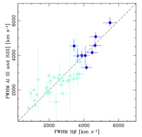
Figure 2: FWHM of Aliii$\lambda$1860 vs FWHM H$\beta$ in km s^-1 for Pop. A sources. The pale blue dots represent quasars from the RQ Pop. A sample of Sulentic et al. (2007), while the blue are from the high-luminosity sample of Sulentic et al. (2017). The dot-dashed line traces the 1:1 relation.

5 Eddington standard candles as distance indicators for cosmology

From the discussion of the previous sections we gather that three conditions are satisfied for xA quasars:

1. constant Eddington ratio $L/L_{\mathrm{Edd}}$; xA quasars radiate close to Eddington limit:

   $$\frac{L}{L_{\mathrm{Edd}}}=\lambda_{\mathrm{E}}\propto\frac{L}{M_{\mathrm{BH}}}$$ (6)

   Note that the precise value or $L/L_{\mathrm{Edd}}$ depends on the normalisation applied for $M_{\mathrm{BH}}$ and on the bolometric correction to compute the bolometric luminosity. Applying widely employed scaling laws, $L/L_{\mathrm{Edd}}$$\lesssim 1$.

2. The assumption of virial motions of the low-ionization BLR, so that the black hole mass $M_{\mathrm{BH}}$ can be expressed by the virial relation (Eq. 1):

   $$M_{\rm BH}=\frac{r_{\mathrm{BLR}}\delta v_{\rm K}^{2}}{G}$$

3. Spectral invariance: for extreme Population A, the ionization parameter $U$ can be written as

   $$U={Q(H)}/{4\pi r_{\mathrm{BLR}}^{2}n_{\mathrm{H}}c}\propto{L}/{r^{2}n_{\mathrm{H}}}$$ (7)

   (Netzer, 2013), where $Q(H)$ is the number of hydrogen ionizing photons. $U$ has to be approximately constant, otherwise we would observe a significant change in the spectral appearance.

5.1 The virial luminosity equation

Taking the three constraints into account, the virial luminosity equation derived by Marziani and Sulentic (2014a) can be written in the form:

$$L(\rm FWHM) = {\mathcal{L}_{\rm 0}}\cdot(\rm FWHM)^{4}_{1000}$$

$$= 7.88\cdot 10^{44}\left(\frac{L}{L_{\mathrm{Edd}}}\right)_{,1}^{2}\cdot\frac{\kappa_{\mathrm{i,0.5}}f_{\mathrm{S,2}}^{2}}{h\bar{\nu}_{\mathrm{i,100eV}}}\frac{1}{(n_{\mathrm{H}}U)_{10^{9.6}}}(\rm FWHM)^{4}_{1000}\,{\rm erg\,s}^{-1}$$

where the energy value has been normalized to 100 eV ($\bar{\nu}_{\mathrm{i,100eV}}\approx 2.42\cdot 10^{16}$ Hz), $\kappa_{\mathrm{i,0.5}}$ is the fraction of bolometric luminosity belonging to the ionizing continuum scaled to 0.5, the product ($n_{\rm H}U$) has been scaled to the typical value $10^{9.6}$cm^-3 (Padovani and Rafanelli, 1988; Matsuoka et al., 2008; Negrete et al., 2012), and the FWHM of the H$\beta$ BC is expressed in units of1000 km s^-1. The $f_{\mathrm{S}}$ is scaled to the value 2 following the determination of Collin et al. (2006). The FWHM of H$\beta$ broad component and of Aliii$\lambda$1860 are hereafter adopted as a virial broadening estimator. Eq. 5.1 implies that, by a simple measurement of the FWHM of a LIL, we can derive a $z-$independent estimate of the accretion luminosity (Marziani and Sulentic, 2014a, c.f. Teerikorpi 2011).

Recent works involved similar ideas concerning the possibility of “virial luminosity” estimates, and confirm that extremely accreting quasars could provide suitable distance indicators because their emission properties appear to be stable with their luminosity scaling with black hole mass at a fixed ratio (Wang et al., 2013; La Franca et al., 2014; Wang et al., 2014a). Eq. 5.1 can be applied to xA quasars only ($L/L_{\mathrm{Edd}}$$\sim$ 1). However, it can be applied to all xA distributed over a wide range of luminosity and redshift, where conventional cosmological distance incdicators are not available (see D’Onofrio and Burigana, 2009; Hook, 2013; Czerny et al., 2018, for reviews concerning distance indicators beyond $z\gtrsim 1$).

The virial luminosity equation is analogous to the Tully-Fisher and the early formulation of the Faber Jackson laws for early- type galaxies (Faber and Jackson, 1976; Tully and Fisher, 1977). We note in passing that galaxies and even clusters of galaxies are virialized systems that show an overall consistency with a law $L\propto\sigma^{\mathrm{n}}$, where $\sigma$ is a measurement of the velocity dispersion and $n\sim 2-4$. Both the Faber and Jackson (1976) and Tully and Fisher (1977) found some application to the determination of the distance scale, especially at low-$z$ (e.g., Dressler et al., 1987, see Czerny et al. 2018 for a recent review). Distance measurements to early-type galaxies can be obtained by applying the relation of the fundamental plane of galaxies (e.g., Saulder et al., 2019) which consider the relation between $\sigma$, structure and luminosity. Galaxies are more complex than quasars due to their non-homology (D’Onofrio et al., 2017). We hope to have minimized structural and physical condition differences by restricting the selection to xA quasars. The factor ${\mathcal{L}_{\rm 0}}$ is most likely affected by intrinsic variations in the spectral energy distribution (SED) of xA sources, as well as by anisotropic emission expected from a thick accretion disk (Wang et al., 2014c). The issue will be briefly discussed in §7.

5.2 Orientation-dependent virial luminosity equation

The effect of orientation can be quantified by assuming that the line broadening is due to an isotropic component + a flattened component whose velocity field projection along the line of sight is $\propto 1/\sin\theta$:

$$\delta v^{2}_{\mathrm{obs}}=\frac{\delta v_{\mathrm{iso}}^{2}}{3}+\delta v_{\mathrm{K}}^{2}\sin^{2}\theta.$$ (9)

The structure factor in the Eq. 5.1 is set to $f_{\rm S}=2$ since Collin et al. (2006) derived values for $f_{\mathrm{S}}\approx$ 2.1 for Pop. A, with a substantial scatter. If we considered a flattened distribution of clouds with an isotropic $\delta v_{\rm iso}$ and a velocity component associated with a rotating flat disk $\delta v_{\rm K}$, the structure factor appearing in Eq. 5.1 can be written as

$$f_{\rm S}=\frac{1}{4\left[\frac{1}{3}\left(\frac{\delta v_{\rm iso}}{\delta v_{\rm K}}\right)^{2}+\sin^{2}\theta\right]}$$ (10)

which can reach values $\gtrsim 1$ if $\kappa=\frac{\delta v_{\rm iso}}{\delta v_{\rm K}}\ll 1$, and if $\theta$ is also small ($\lesssim 30$ deg). The assumption $f_{\rm S}=2$ implies that we are seeing a highly flattened system (if all parameters in Eq. 5.1 are set to their appropriate values); an isotropic velocity field would yield $f_{\rm S}=0.75$.

The virial luminosity equation may be rewritten in the form:

$$L({\rm FWHM}) = {{\mathcal{L}_{\rm 0}}}f^{-2}_{\rm S}(\delta v_{\rm K})^{4}$$

$$= {4^{2}{\mathcal{L}^{\bullet}_{\rm 0}}(\delta v_{\rm K})^{4}}{\left[\frac{\kappa^{2}}{3}+\sin^{2}\theta\right]}^{2}=4^{2}L_{\rm vir}{\left[\frac{\kappa^{2}}{3}+\sin^{2}\theta\right]}^{2},$$

where $L_{\rm vir}$ is the true virial luminosity (which implies $f_{\rm S}=1$) with ${\mathcal{L}^{\bullet}_{\rm 0}}=\frac{1}{4}{\mathcal{L}_{\rm 0}}$, since ${\mathcal{L}_{\rm 0}}$ was scaled to $f_{\rm S}=2$.

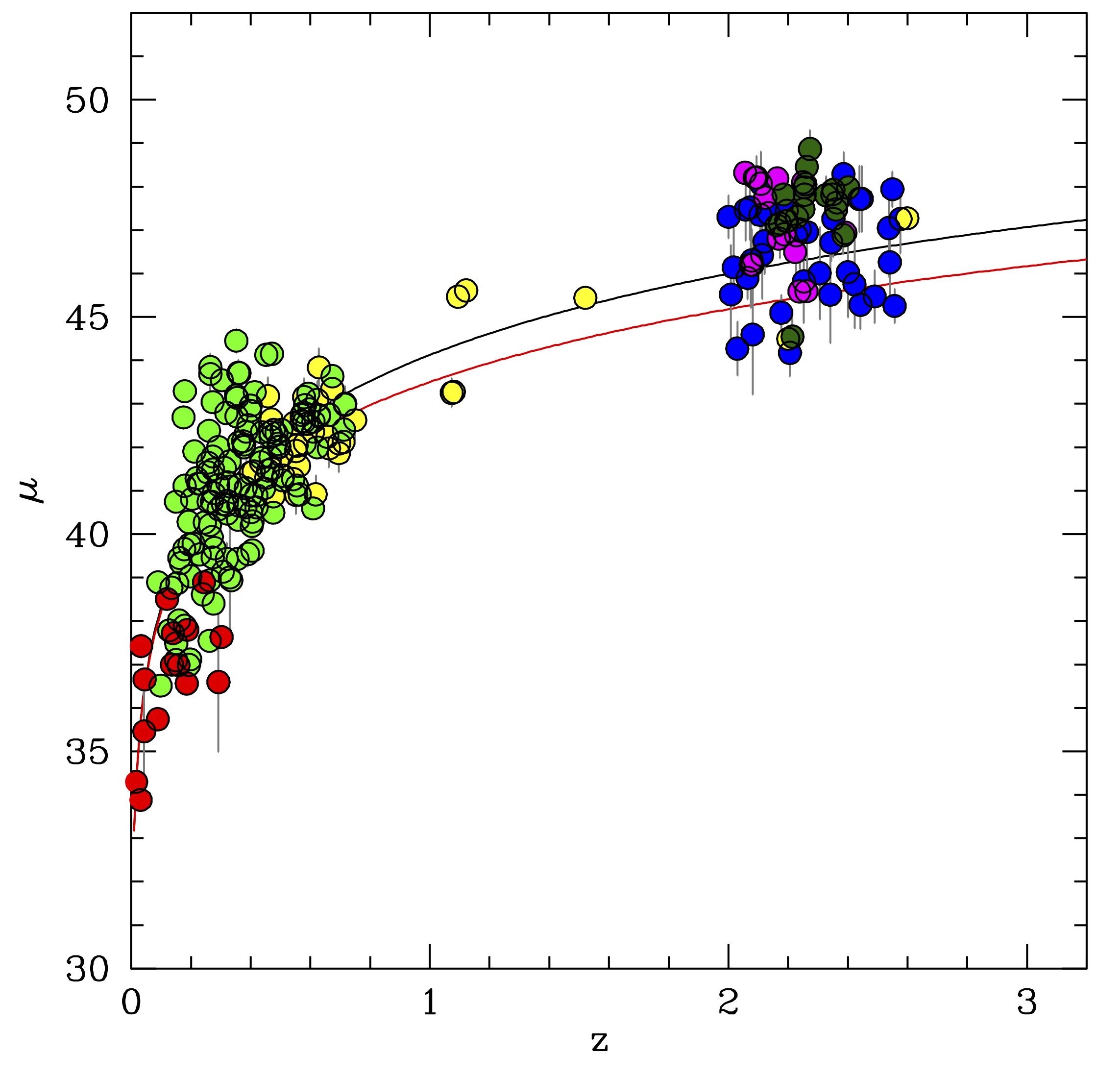
Figure 3: Hubble diagram (distance modulus $\mu$ vs redshift $z$) for several samples of xA quasars using virial luminosity distances from the FWHM of H$\beta$ and Aliii$\lambda$1860. Data points are color-coded according to sample and line employed: blue ($\bullet$): Marziani and Sulentic (2014a) Aliii$\lambda$1860; yellow ($\bullet$): Marziani and Sulentic (2014a) H$\beta$; green ($\bullet$): Negrete et al. (2018) H$\beta$; red ($\bullet$): Du et al. (2016) H$\beta$; dark green ($\bullet$): Sniegowska et al. in preparation; magenta ($\bullet$): Martínez-Aldama et al. (2018). The continuous lines trace the prediction for concordance $\Lambda$CDM (black) the Einstein-de Sitter (red) cosmology.

6 The Hubble diagram for quasars

6.1 The basic

Following Weinberg (1972, 2008) the luminosity distance $d_{\rm L}$ can be written as:

$$d_{L}(z;\Omega_{M},\Omega_{\Lambda},H_{0}) = \frac{d_{\rm H}(1+z)}{\sqrt{|\kappa|}}\cdot\;\;\;$$

$${S}\!\left(\sqrt{|{\kappa}|}\int_{0}^{z}\left[(1+z^{\prime})^{2}(1+\Omega_{M}z^{\prime})-z^{\prime}(2+z^{\prime})\Omega_{\Lambda}\right]^{-\frac{1}{2}}dz^{\prime}\right),$$

where $\Omega_{M}$  is the energy density associated to matter and $\Omega_{\Lambda}$  the energy density associated to $\Lambda$, and $d_{\rm H}\equiv\frac{c}{H_{0}}=3000\,h^{-1}~{}{\rm Mpc}=9.26\times 10^{25}\,h^{-1}~{}{\rm m}$, with $\log\ d_{\mathrm{H}}\approx 28.12$ [cm].

If $\Omega_{M}+\Omega_{\Lambda}>1$, ${S}(x)$ is defined as $\sin(x)$ and $\kappa=1-\Omega_{M}-\Omega_{\Lambda}$; for $\Omega_{M}+\Omega_{\Lambda}<1$, ${S}(x)=\sinh(x)$ and $\kappa$ as above; and for $\Omega_{M}+\Omega_{\Lambda}=1$, ${S}(x)=x$ and $\kappa=1$.

The equation of Perlmutter et al. (1997) has been obtained by posing $\Omega_{k}+\Omega_{\Lambda}+\Omega_{\mathrm{M}}=1$, where $\Omega_{k}$ is the energy density associated with the curvature of space-time. The luminosity distance $d_{\rm L}=d_{\rm C}\cdot(1+z)$ can be computed in practice from:

$$d_{\rm C}=d_{\rm H}\,\int_{0}^{z}\frac{dz^{\prime}}{E(z^{\prime})}$$ (13)

with

$$d_{\rm H}\equiv\frac{c}{H_{0}}=3000\,h^{-1}~{}{\rm Mpc}=9.26\times 10^{25}\,h^{-1}~{}{\rm m}$$ (14)

with $\log\ d_{\mathrm{H}}\approx 28.12$ [cm] and

$$E(z)\equiv\sqrt{\Omega_{\rm M}\,(1+z)^{3}+\Omega_{k}\,(1+z)^{2}+\Omega_{\Lambda}}$$ (15)

The distance modulus $\mu$ is defined by

$$\mu\equiv 5\,\log\left(\frac{d_{\rm L}(H_{0},\Omega_{\rm M},\Omega_{k},\Omega_{\Lambda},z)}{10~{}{\rm pc}}\right),$$ (16)

that is $\mu=\log d_{\mathrm{L}}(H_{0},\Omega_{\rm M},\Omega_{k},\Omega_{\Lambda},z)+5$, where the constant +5 becomes +25 if distances are expressed in Mpc (Lang, 1980).

The distance modulus $\mu$ computed from the virial equation yielding $L(\delta v)$ can be written as:

$$\mu=2.5[\log L(\delta v)-BC]-2.5\log(f_{\lambda}\lambda)-2.5\log(4\pi\delta_{\mathrm{10pc}}^{2})+5\cdot\log(1+z)$$ (17)

where the constant $-2.5\log(4\pi\delta_{\mathrm{10pc}}^{2})$ =-100.19, with $\delta_{\mathrm{10pc}}\approx 3.08\cdot 10^{19}$  the distance of 10pc expressed in cm. The $f_{\lambda}\lambda$ can be the flux at 5100 Å for the H$\beta$ sample, or the flux at 1700 Å if the $\delta v$=FWHM comes from the Aliii$\lambda$1860 and Siiii]$\lambda$1892 lines. The bolometric correction $BC$ has also to be changed accordingly.

The $\delta\mu=\mu_{\mathrm{vir}}-\mu(z;\Omega_{M},\Omega_{\Lambda},H_{0})$ can be written as:

$$\delta\mu=2.5[\log L(\delta v)-BC]-2.5\log(f_{\lambda}\lambda)+5\cdot\log(1+z)-5\log d_{\rm L}(H_{0},\Omega_{\rm M},\Omega_{k},\Omega_{\Lambda},z)$$ (18)

Following the notation of Marziani and Sulentic (2014a) who wrote the comoving distance as $d=c/H_{0}\mathcal{F}(\Omega_{\rm M},\Omega_{k},\Omega_{\Lambda},z)$, we derive:

$$\mu \approx 5\cdot\left(\log\frac{c}{H_{0}}+\log\mathcal{F}(\Omega_{\rm M},\Omega_{k},\Omega_{\Lambda},z)\right)$$

$$-5\cdot\log\delta_{\mathrm{10pc}}+5\cdot\log(1+z)$$

If we equate Equations 17 and 6.1 above, we obtain:

$$2.5[\log L(\delta v)-BC]-2.5\log(f_{\lambda}\lambda)-5\log\delta_{\mathrm{10pc}}$$ (20)

$$-2.5\log 4\pi+5\cdot\log(1+z) =$$

$$5\cdot\left(\log\frac{c}{H_{0}}+\log\mathcal{F}(\Omega_{\rm M},\Omega_{k},\Omega_{\Lambda},z)\right)$$

$$-5\cdot\log\delta_{\mathrm{10pc}}+5\cdot\log(1+z).$$

Simplifying:

$${[L(\delta v)-BC]}=4\pi\left(\frac{c}{H_{0}}{\mathcal{F}}(\Omega_{\rm M},\Omega_{k},\Omega_{\Lambda},z)\right)^{2}{(f_{\lambda}\lambda),}$$ (21)

we recover the expression used by Marziani and Sulentic (2014a) who used only luminosity and did not give any expression for $\mu$. Note that ${(f_{\lambda}\lambda)}$ refers to the rest frame fluxes (the term $(1+z)^{2}$ appears in both side of the equations, for the virial luminosity and for the distance modulus where the luminosity distance was used).

6.2 Results

The Hubble diagram of Fig. 3 includes sources from Marziani and Sulentic (2014a), with both H$\beta$ and Aliii$\lambda$1860, and is supplemented by SDSS low-luminosity xA sources at low $z$ covering the H$\beta$ range (Negrete et al., 2018), by new high-$z$ quasar observations at redshift $2\lesssim z<\lesssim 3$ that were observed with the OSIRIS camera at the GTC, covering the $\lambda$1900 Å blend and hence Aliii$\lambda$1860 (Martínez-Aldama et al., 2018). An additional sample at very low-$z$ is the one of the xA sources considered for the Du et al. (2016) fundamental plane. Preliminary results of the Aliii$\lambda$1860 measurements for $\approx$ 15 quasars (Sniegowska et al. 2019, in preparation) are also shown. The value of $\log$ ${\mathcal{L}_{0}}\approx$ 45.06 was used in the computation of the distance modulus $\mu$ for this work. The plots in Fig. 3 involves a total of 253 sources and indicate a scatter $\delta\mu\approx$ 1.2 mag. A similar result was shown with 169 xA quasars by Marziani et al. (2017). The plot of Fig. 3 shows that even our heterogeneous sample joining H$\beta$ and Aliii$\lambda$1860 based sub-samples already rules out extreme Universes such as the Einstein-de Sitter Universe ($\Omega_{\mathrm{M}}=1,\Omega_{\Lambda}=0$, red line in Fig. 3), which under-predicts $\mu$ values at high $z$ by $\approx 1$ mag with respect to concordance. The inclusion of the Aliii$\lambda$1860 has been instrumental to the extension of the Hubble diagram to redshifts $\gtrsim 1$. Observations of H$\beta$ at redshift $\gtrsim$ 1 are available for several hundreds of quasars (e.g., Coatman et al., 2016; Shen, 2016); this means that only a few tens of spectra may be available from literature, if the observations are restricted to xA source and high S/N is requested. An additional virial broadening estimator is needed. The Aliii$\lambda$1860  line can be measured from SDSS survey up to $z\gtrsim 4$. Fig. 2 shows preliminary results for a sample of Population A sources. The evidence collected so far suggests that the correlation should remain valid for most xA sources (a few notable exceptions are known; for example HE0359-3959, Martínez-Aldama et al. 2017). The suitability of Aliii$\lambda$1860 as a virial broadening estimator will be further explored in eventual works.

The Hubble diagram for quasars restricted to the 92 sources of Marziani and Sulentic (2014a) was also consistent with concordance $\Lambda$CDM provided some constraints on $\Omega_{\mathrm{M}}:0.19^{+0.16}_{-0.08}$. The redshift range 2 - 3 is highly sensitive to $\Omega_{\mathrm{M}}$. The new sample is consistent with the old one and allows to set more stringent limits to $\Omega_{\mathrm{M}}\approx$ 0.30${}^{+0.06}_{-0.06}$ via a standard Bayesian least square fit, employing a sample with no restriction on data (i.e., including low-S/N Aliii$\lambda$1860 spectra and a few quasars at $z$ in the range 2.6 —3 not shown in Fig. 3).

7 Discussion

In this paper we have described the method developed by Marziani and Sulentic (2014a) in more detail, presented an expanded Hubble diagram with more objects with respect to the one presented by Marziani et al. (2017), as well as an updated (but still preliminary estimate) of $\Omega_{\mathrm{M}}$ and the Hubble diagram with concordance and Einstein-de Sitter cosmologies, just to illustrate the sensitivity of the method to cosmological parameter changes. It should be also noted that a comparison between the constraints set by the supernova photometric survey described by Campbell et al. (2013) and a mock sample of 400 quasars with rms = 0.3 uniformly covering the $z$ range $0.1-3$ that assumes concordance cosmology (shaded contours in Fig. 4 of Marziani and Sulentic 2014b) emphasizes the potential ability of the quasar sample to better constrain $\Omega_{\mathrm{M}}$.

An elementary error budget suggests that the main uncertainty is associated with FWHM measurement errors and with uncertainty in the structure factor (Marziani and Sulentic, 2014a; Negrete et al., 2018). The broad profile of both LILs and HILs in each quasar spectrum can be modeled by considering two main components, the H$\beta$ BC and the blueshifted component BLUE (§3). Results shown in Fig. 3 refer to H$\beta$ BC profiles whose FWHM has been corrected for the effect of BLUE via a multi-component fit, as described in Negrete et al. (2018). The H$\beta$ BLUE affects however the H$\beta$ FWHM only at $\approx$ 10% level, with an effect that should be $\lesssim$ 0.3 dex. Vetting the sample on strongest Feii and weakest [Oiii]$\lambda\lambda$4959,5007 emitters reduces the scatter but only slightly (Negrete et al., 2018).

Negrete et al. (2018) have convincingly shown that orientation effects are at the origin of a large fraction of the scatter if lines are emitted in a flattened system ($\kappa\lesssim 0.2$). The difference between virial and concordance luminosity estimates can be zeroed if the structure factor is assumed to be dependent on angle $\theta$ in the form given by Eq. 10. The resulting distribution of $\theta$ values ranges from 0 to 50 with a peak around $\theta\approx 18$. The range of viewing angles in the sample of Negrete et al. (2018) is actually modest. The effect of anisotropy from a geometrically and optically thick disk on the SED is not extremely strong within $\theta\lesssim 30$, approximately around 0.2 dex, following the models of anisotropic emission of Wang et al. (2014c). The actual effect on virial luminosity estimates could be even less than that, as the dispersion in the distribution of $\theta$ in the sample of Negrete et al. (2018) is just 7 degrees, which implies that most sources are seen in a viewing angle range between 10 and 30 degrees. Fig. 4 of Wang et al. (2014c) indicates that different $\theta$ should lead to an increase of the dispersion of a few 0.01 dex around the luminosity expected for 20 degrees at optical wavelengths. This will mainly affect the continuum $\lambda f_{\lambda}$ that we receive entering in Eq. 17.

The presence of a thick disk implies self-shadowing effects, and that the line emitting gas might not be exposed to the same ionizing continuum that is seen by the observer. This second effect related to the disk anisotropy is especially severe if the line emitting gas is located close to the equatorial plane of the disk: in this case, following Wang et al. (2014c), we expect a drastic reduction of the number of ionizing photons which would affect ${\mathcal{L}_{\rm 0}}$. Precisely quantifying the effect on line emission is not trivial, as it depends on the distribution of the line emitting gas around the equatorial plane of the disk, in terms of both angular and radial distance (Du and Wang, 2019), the black hole mass as well as the accretion disk model. Differences in the accretion disk SED are also expected from object to object because of different black hole spins (Wang et al., 2014b). The spin and the anisotropy effects on ${\mathcal{L}_{\rm 0}}$ should be considered in an eventual work, but there is a basic point that we want to remark about the usability of Eq. 5.1 for cosmology.

The SED parameters entering in the relation for the virial luminosity are $\bar{\nu}_{\mathrm{i}}$, $\kappa_{\mathrm{i}}$, and more indirectly, $n_{\mathrm{H}}U$. The ionizing photon flux $n_{\mathrm{H}}U$ shows remarkably small changes along the MS (i.e., even without restricting the attention to xA sources), as shown by the various estimates reported in Table 4 of Negrete et al. (2012): it cannot change by a large factor, otherwise the emission line spectrum would change dramatically (Panda et al., 2018, 2019). The other SED-related parameters appear as $\kappa_{\mathrm{i}}/\bar{\nu}_{\mathrm{i}}$, and are qualitatively affected in the same way by a change of the ionizing continuum. Explorative computations using CLOUDY (Ferland et al., 2017) indicate that the ratio $\kappa_{\mathrm{i}}/\bar{\nu}_{\mathrm{i}}$ decreases by a factor $\approx 1.2$ for a change of $\theta$ from $\theta\lesssim 20-30$ to $\theta\sim 50-70$. This condition could be appropriate if the “walls” of the thick disk are illuminating the low-ionization part of the BLR. Object-by-object differences may add scatter in ${\mathcal{L}_{\rm 0}}$, therefore contribution to the dispersion observed in the Hubble diagram of Fig. 3.

The issue of anisotropy and of other factors affecting the ${\mathcal{L}_{\rm 0}}$ term multiplying the line width in Eq. 5.1 brings to the attention the possibility of structural changes with redshift and luminosity although it is at least conceivable that the accretion mode at high rates is giving rise to a stable and reproducible structure. This consideration is supported by the stability of xA sources at least in the optical domain (Du et al., 2018), as shown by the small amplitude of continuum variations detected in dedicated reverberation mapping campaigns, and by the similarity of low-ionization emission line profiles over a wide range of redshift and luminosity.

Summing up, we can say that the proper calibration of the data for cosmology will need large samples of quasar spectra covering the rest frame optical and UV, at high S/N, over a wide range of redshift. This is a conditio sine qua non to test for systematic sources of errors and hence for the effective exploitation of quasar data for cosmology applying the virial luminosity equation at $z\gtrsim 1$.

8 Conclusion

The quasar MS has allowed us to isolate sources which are the highest radiators among quasars. This is already an important feat, as xAs can then be selected by the application of simple criteria based on optical and UV emission line ratios. xA quasars show a relatively high prevalence (10%) and are easily recognizable in the redshift range 1 – 5. The present work illustrated several key aspects of the method, and provided the virial luminosity equation dependent from the viewing angle in an explicit form (a result of Negrete et al. 2018). However, several additional caveats need to addressed in subsequent work: the reliability of Aliii$\lambda$1860 as a virial broadening estimator and, generally speaking, the inter-calibration of the data obtained in the rest frame UV and optical domain, as well as the effect of anisotropic continuum emission expected for xA sources. xA might be suitable as Eddington standard candles especially if orientation and systematic effects as a function of redshift and luminosity can be identified and accounted for.

Author Contributions

PM wrote the paper with the assistance of DD; PM and JAdD did the Hubble diagram analysis and JAdD contributed the $\Omega_{\mathrm{M}}$ estimate. All other authors (part of the extreme team) sent comments and/or contributed to some extent during the development of the project.

Funding

References

- Abramowicz et al. (1988) Abramowicz, M. A., Czerny, B., Lasota, J. P., and Szuszkiewicz, E. (1988). Slim accretion disks. Astroph. J. 332, 646–658. 10.1086/166683
- Adhikari et al. (2016) Adhikari, T. P., Różańska, A., Czerny, B., Hryniewicz, K., and Ferland, G. J. (2016). The Intermediate-line Region in Active Galactic Nuclei. Astroph. J. 831, 68. 10.3847/0004-637X/831/1/68
- Antonucci (1993) Antonucci, R. (1993). Unified models for active galactic nuclei and quasars. Ann. Rev. Astron. Astroph. 31, 473–521. 10.1146/annurev.aa.31.090193.002353
- Azzalini and Regoli (2012) Azzalini, A. and Regoli, G. (2012). Some properties of skew-symmetric distributions. Ann. Inst. Statist. Math. 64, 857–879. 10.1007/s10463-011-0338-5
- Barth et al. (2013) Barth, A. J., Pancoast, A., Bennert, V. N., Brewer, B. J., Canalizo, G., Filippenko, A. V., et al. (2013). The Lick AGN Monitoring Project 2011: Fe II Reverberation from the Outer Broad-line Region. Astroph. J. 769, 128. 10.1088/0004-637X/769/2/128
- Bentz et al. (2013) Bentz, M. C., Denney, K. D., Grier, C. J., Barth, A. J., Peterson, B. M., Vestergaard, M., et al. (2013). The Low-luminosity End of the Radius-Luminosity Relationship for Active Galactic Nuclei. Astroph. J. 767, 149. 10.1088/0004-637X/767/2/149
- Bisogni et al. (2017) Bisogni, S., di Serego Alighieri, S., Goldoni, P., Ho, L. C., Marconi, A., Ponti, G., et al. (2017). Simultaneous detection and analysis of optical and ultraviolet broad emission lines in quasars at z 2.2. Astron. Astroph. 603, A1. 10.1051/0004-6361/201630143
- Boroson and Green (1992) Boroson, T. A. and Green, R. F. (1992). The emission-line properties of low-redshift quasi-stellar objects. ApJS 80, 109–135. 10.1086/191661
- Brotherton et al. (1994) Brotherton, M. S., Wills, B. J., Francis, P. J., and Steidel, C. C. (1994). The intermediate line region of QSOs. Astroph. J. 430, 495–504. 10.1086/174425
- Campbell et al. (2013) Campbell, H., D’Andrea, C. B., Nichol, R. C., Sako, M., Smith, M., Lampeitl, H., et al. (2013). Cosmology with Photometrically Classified Type Ia Supernovae from the SDSS-II Supernova Survey. Astroph. J. 763, 88. 10.1088/0004-637X/763/2/88
- Coatman et al. (2016) Coatman, L., Hewett, P. C., Banerji, M., and Richards, G. T. (2016). C iv emission-line properties and systematic trends in quasar black hole mass estimates. Mon. Not. R. Astron. Soc. 461, 647–665. 10.1093/mnras/stw1360
- Coatman et al. (2017) Coatman, L., Hewett, P. C., Banerji, M., Richards, G. T., Hennawi, J. F., and Prochaska, J. X. (2017). Correcting C IV-based virial black hole masses. Mon. Not. R. Astron. Soc. 465, 2120–2142. 10.1093/mnras/stw2797
- Collin et al. (2006) Collin, S., Kawaguchi, T., Peterson, B. M., and Vestergaard, M. (2006). Systematic effects in measurement of black hole masses by emission-line reverberation of active galactic nuclei: Eddington ratio and inclination. A&Ap 456, 75–90. 10.1051/0004-6361:20064878
- Collin-Souffrin et al. (1988) Collin-Souffrin, S., Dyson, J. E., McDowell, J. C., and Perry, J. J. (1988). The environment of active galactic nuclei - I. A two-component broad emission line model. Mon. Not. R. Astron. Soc. 232, 539–550. 10.1093/mnras/232.3.539
- Cracco et al. (2016) Cracco, V., Ciroi, S., Berton, M., Di Mille, F., Foschini, L., La Mura, G., et al. (2016). A spectroscopic analysis of a sample of narrow-line Seyfert 1 galaxies selected from the Sloan Digital Sky Survey. Mon. Not. R. Astron. Soc. 462, 1256–1280. 10.1093/mnras/stw1689
- Czerny et al. (2018) Czerny, B., Beaton, R., Bejger, M., Cackett, E., Dall’Ora, M., Holanda, R. F. L., et al. (2018). Astronomical Distance Determination in the Space Age. Secondary Distance Indicators. Space Science Reviews 214, #32. 10.1007/s11214-018-0466-9
- Diamond-Stanic et al. (2009) Diamond-Stanic, A. M., Fan, X., Brandt, W. N., Shemmer, O., Strauss, M. A., Anderson, S. F., et al. (2009). High-redshift SDSS Quasars with Weak Emission Lines. Astroph. J. 699, 782–799. 10.1088/0004-637X/699/1/782
- D’Onofrio and Burigana (2009) D’Onofrio, M. and Burigana, C. (2009). Questions of Modern Cosmology: Galileo’s Legacy (Springer Verlag). 10.1007/978-3-642-00792-7
- D’Onofrio et al. (2017) D’Onofrio, M., Cariddi, S., Chiosi, C., Chiosi, E., and Marziani, P. (2017). On the Origin of the Fundamental Plane and Faber-Jackson Relations: Implications for the Star Formation Problem. Astroph. J. 838, 163. 10.3847/1538-4357/aa6540
- Dressler et al. (1987) Dressler, A., Lynden-Bell, D., Burstein, D., Davies, R. L., Faber, S. M., Terlevich, R., et al. (1987). Spectroscopy and Photometry of Elliptical Galaxies. I. New Distance Estimator. Astroph. J. 313, 42. 10.1086/164947
- Du and Wang (2019) Du, P. and Wang, J.-M. (2019). The Radius-Luminosity Relationship Depends on Optical Spectra in Active Galactic Nuclei. Astroph. J. 886, 42. 10.3847/1538-4357/ab4908
- Du et al. (2016) Du, P., Wang, J.-M., Hu, C., Ho, L. C., Li, Y.-R., and Bai, J.-M. (2016). The Fundamental Plane of the Broad-line Region in Active Galactic Nuclei. Astroph. J. Lett. 818, L14. 10.3847/2041-8205/818/1/L14
- Du et al. (2018) Du, P., Zhang, Z.-X., Wang, K., Huang, Y.-K., Zhang, Y., Lu, K.-X., et al. (2018). Supermassive Black Holes with High Accretion Rates in Active Galactic Nuclei. IX. 10 New Observations of Reverberation Mapping and Shortened H Lags. Astroph. J. 856, 6. 10.3847/1538-4357/aaae6b
- Elvis (2000) Elvis, M. (2000). A Structure for Quasars. Astroph. J. 545, 63–76. 10.1086/317778
- Faber and Jackson (1976) Faber, S. M. and Jackson, R. E. (1976). Velocity dispersions and mass-to-light ratios for elliptical galaxies. Astroph. J. 204, 668–683. 10.1086/154215
- Ferland et al. (2017) Ferland, G. J., Chatzikos, M., Guzmán, F., Lykins, M. L., van Hoof, P. A. M., Williams, R. J. R., et al. (2017). The 2017 Release Cloudy. RevMexA&Ap 53, 385–438
- Ferland et al. (2009) Ferland, G. J., Hu, C., Wang, J., Baldwin, J. A., Porter, R. L., van Hoof, P. A. M., et al. (2009). Implications of Infalling Fe II-Emitting Clouds in Active Galactic Nuclei: Anisotropic Properties. Astroph. J. Lett. 707, L82–L86. 10.1088/0004-637X/707/1/L82
- Fraix-Burnet et al. (2017) Fraix-Burnet, D., Marziani, P., D’Onofrio, M., and Dultzin, D. (2017). The phylogeny of quasars and the ontogeny of their central black holes. Frontiers in Astronomy and Space Sciences 4, 1. 10.3389/fspas.2017.00001
- Hook (2013) Hook, I. M. (2013). Supernovae and cosmology with future European facilities. Royal Society of London Philosophical Transactions Series A 371, 20282. 10.1098/rsta.2012.0282
- Kaspi et al. (2000) Kaspi, S., Smith, P. S., Netzer, H., Maoz, D., Jannuzi, B. T., and Giveon, U. (2000). Reverberation Measurements for 17 Quasars and the Size-Mass-Luminosity Relations in Active Galactic Nuclei. Astroph. J. 533, 631–649. 10.1086/308704
- Kovačević-Dojčinović and Popović (2015) Kovačević-Dojčinović, J. and Popović, L. Č. (2015). The Connections Between the UV and Optical Fe ii Emission Lines in Type 1 AGNs. Astroph. J. Supp. 221, 35. 10.1088/0067-0049/221/2/35
- La Franca et al. (2014) La Franca, F., Bianchi, S., Ponti, G., Branchini, E., and Matt, G. (2014). A New Cosmological Distance Measure Using Active Galactic Nucleus X-Ray Variability. Astroph. J. Lett. 787, L12. 10.1088/2041-8205/787/1/L12
- Lang (1980) Lang, K. R. (1980). Astrophysical Formulae. A Compendium for the Physicist and Astrophysicist. (Springer Verlag, Berlin-Heidelberg)
- Leighly (2004) Leighly, K. M. (2004). Hubble Space Telescope STIS Ultraviolet Spectral Evidence of Outflow in Extreme Narrow-Line Seyfert 1 Galaxies. II. Modeling and Interpretation. ApJ 611, 125–152. 10.1086/422089
- Leighly and Moore (2004) Leighly, K. M. and Moore, J. R. (2004). Hubble Space Telescope STIS Ultraviolet Spectral Evidence of Outflow in Extreme Narrow-Line Seyfert 1 Galaxies. I. Data and Analysis. Astroph. J. 611, 107–124. 10.1086/422088
- Li et al. (2018) Li, Y.-R., Songsheng, Y.-Y., Qiu, J., Hu, C., Du, P., Lu, K.-X., et al. (2018). Supermassive Black Holes with High Accretion Rates in Active Galactic Nuclei. VIII. Structure of the Broad-line Region and Mass of the Central Black Hole in Mrk 142. Astroph. J. 869, 137. 10.3847/1538-4357/aaee6b
- Li et al. (2013) Li, Y.-R., Wang, J.-M., Ho, L. C., Du, P., and Bai, J.-M. (2013). A Bayesian Approach to Estimate the Size and Structure of the Broad-line Region in Active Galactic Nuclei Using Reverberation Mapping Data. Astroph. J. 779, 110. 10.1088/0004-637X/779/2/110
- Marinello et al. (2016) Marinello, A. O. M., Rodriguez-Ardila, A., Garcia-Rissmann, A., Sigut, T. A. A., and Pradhan, A. K. (2016). The FeII emission in active galactic nuclei: excitation mechanisms and location of the emitting region. ArXiv e-prints
- Martínez-Aldama et al. (2017) Martínez-Aldama, M. L., Del Olmo, A., Marziani, P., Negrete, C. A., Dultzin, D., and Martínez-Carballo, M. A. (2017). He0359-3959: An extremely radiating quasar. Frontiers in Astronomy and Space Sciences 4, 29. 10.3389/fspas.2017.00029
- Martínez-Aldama et al. (2018) Martínez-Aldama, M. L., Del Olmo, A., Marziani, P., Sulentic, J. W., Negrete, C. A., Dultzin, D., et al. (2018). Highly accreting quasars at high redshift. Frontiers in Astronomy and Space Sciences 4, 65. 10.3389/fspas.2017.00065
- Marziani et al. (2018a) Marziani, P., del Olmo, A., D’ Onofrio, M., Dultzin, D., Negrete, C. A., Martiinez-Aldama, M. L., et al. (2018a). Narrow-line Seyfert 1s: what is wrong in a name? ArXiv e-prints
- Marziani et al. (2019) Marziani, P., del Olmo, A., Martínez-Carballo, M. A., Martínez-Aldama, M. L., Stirpe, G. M., Negrete, C. A., et al. (2019). Black hole mass estimates in quasars. A comparative analysis of high- and low-ionization lines. Astron. Astroph. 627, A88. 10.1051/0004-6361/201935265
- Marziani et al. (2018b) Marziani, P., Dultzin, D., Sulentic, J. W., Del Olmo, A., Negrete, C. A., Martinez-Aldama, M. L., et al. (2018b). A main sequence for quasars. Frontiers in Astronomy and Space Sciences 5, 6
- Marziani et al. (2017) Marziani, P., Negrete, C. A., Dultzin, D., Martinez-Aldama, M. L., Del Olmo, A., Esparza, D., et al. (2017). Highly accreting quasars: a tool for cosmology? In IAU Symposium. vol. 324 of IAU Symposium, 245–246. 10.1017/S1743921316012655
- Marziani and Sulentic (2014a) Marziani, P. and Sulentic, J. W. (2014a). Highly accreting quasars: sample definition and possible cosmological implications. Mon. Not. R. Astron. Soc. 442, 1211–1229. 10.1093/mnras/stu951
- Marziani and Sulentic (2014b) Marziani, P. and Sulentic, J. W. (2014b). Quasars and their emission lines as cosmological probes. Advances in Space Research 54, 1331–1340. 10.1016/j.asr.2013.10.007
- Marziani et al. (1996) Marziani, P., Sulentic, J. W., Dultzin-Hacyan, D., Calvani, M., and Moles, M. (1996). Comparative Analysis of the High- and Low-Ionization Lines in the Broad-Line Region of Active Galactic Nuclei. ApJS 104, 37–+. 10.1086/192291
- Marziani et al. (2010) Marziani, P., Sulentic, J. W., Negrete, C. A., Dultzin, D., Zamfir, S., and Bachev, R. (2010). Broad-line region physical conditions along the quasar eigenvector 1 sequence. Mon. Not. R. Astron. Soc. 409, 1033–1048. 10.1111/j.1365-2966.2010.17357.x
- Marziani et al. (2009) Marziani, P., Sulentic, J. W., Stirpe, G. M., Zamfir, S., and Calvani, M. (2009). VLT/ISAAC spectra of the H region in intermediate-redshift quasars. III. H broad-line profile analysis and inferences about BLR structure. A&Ap 495, 83–112. 10.1051/0004-6361:200810764
- Marziani et al. (2001) Marziani, P., Sulentic, J. W., Zwitter, T., Dultzin-Hacyan, D., and Calvani, M. (2001). Searching for the Physical Drivers of the Eigenvector 1 Correlation Space. ApJ 558, 553–560. 10.1086/322286
- Matsuoka et al. (2008) Matsuoka, Y., Kawara, K., and Oyabu, S. (2008). Low-Ionization Emission Regions in Quasars: Gas Properties Probed with Broad O I and Ca II Lines. ApJ 673, 62–68. 10.1086/524193
- Mineshige et al. (2000) Mineshige, S., Kawaguchi, T., Takeuchi, M., and Hayashida, K. (2000). Slim-Disk Model for Soft X-Ray Excess and Variability of Narrow-Line Seyfert 1 Galaxies. Publ. Astron. Soc. Japan 52, 499–508
- Negrete et al. (2012) Negrete, A., Dultzin, D., Marziani, P., and Sulentic, J. (2012). BLR Physical Conditions in Extreme Population A Quasars: a Method to Estimate Central Black Hole Mass at High Redshift. ApJ 757, 62
- Negrete et al. (2018) Negrete, C. A., Dultzin, D., Marziani, P., Esparza, D., Sulentic, J. W., del Olmo, A., et al. (2018). Highly accreting quasars: The SDSS low-redshift catalog. Astron. Astroph. 620, A118. 10.1051/0004-6361/201833285
- Netzer (2013) Netzer, H. (2013). The Physics and Evolution of Active Galactic Nuclei (Cambridge University Press)
- Netzer and Marziani (2010) Netzer, H. and Marziani, P. (2010). The Effect of Radiation Pressure on Emission-line Profiles and Black Hole Mass Determination in Active Galactic Nuclei. Astroph. J. 724, 318–328. 10.1088/0004-637X/724/1/318
- Padovani and Rafanelli (1988) Padovani, P. and Rafanelli, P. (1988). Mass-luminosity relationships and accretion rates for Seyfert 1 galaxies and quasars. Astron. Astroph. 205, 53–70
- Pancoast et al. (2014) Pancoast, A., Brewer, B. J., and Treu, T. (2014). Modelling reverberation mapping data - I. Improved geometric and dynamical models and comparison with cross-correlation results. Mon. Not. R. Astron. Soc. 445, 3055–3072. 10.1093/mnras/stu1809
- Panda et al. (2018) Panda, S., Czerny, B., Adhikari, T. P., Hryniewicz, K., Wildy, C., Kuraszkiewicz, J., et al. (2018). Modeling of the Quasar Main Sequence in the Optical Plane. Astroph. J. 866, 115. 10.3847/1538-4357/aae209
- Panda et al. (2019) Panda, S., Marziani, P., and Czerny, B. (2019). The Quasar Main Sequence Explained by the Combination of Eddington Ratio, Metallicity, and Orientation. Astroph. J. 882, 79. 10.3847/1538-4357/ab3292
- Perlmutter et al. (1997) Perlmutter, S., Gabi, S., Goldhaber, G., Goobar, A., Groom, D. E., Hook, I. M., et al. (1997). Measurements of the Cosmological Parameters Omega and Lambda from the First Seven Supernovae at Z ¿= 0.35. Astroph. J. 483, 565. 10.1086/304265
- Popović et al. (2002) Popović, L. Č., Mediavilla, E. G., Kubičela, A., and Jovanović, P. (2002). Balmer lines emission region in NGC 3516: Kinematical and physical properties. Astron. Astroph. 390, 473–480. 10.1051/0004-6361:20020724
- Proga et al. (2000) Proga, D., Stone, J. M., and Kallman, T. R. (2000). Dynamics of Line-driven Disk Winds in Active Galactic Nuclei. Astroph. J. 543, 686–696. 10.1086/317154
- Richards et al. (2011) Richards, G. T., Kruczek, N. E., Gallagher, S. C., Hall, P. B., Hewett, P. C., Leighly, K. M., et al. (2011). Unification of Luminous Type 1 Quasars through C IV Emission. Astron. J. 141, 167–+. 10.1088/0004-6256/141/5/167
- Saulder et al. (2019) Saulder, C., Steer, I., Snaith, O., and Park, C. (2019). Distance measurements to early-type galaxies by improving the fundamental plane. arXiv e-prints , arXiv:1905.12970
- Sa̧dowski et al. (2014) Sa̧dowski, A., Narayan, R., McKinney, J. C., and Tchekhovskoy, A. (2014). Numerical simulations of super-critical black hole accretion flows in general relativity. Mon. Not. R. Astron. Soc. 439, 503–520. 10.1093/mnras/stt2479
- Shen (2016) Shen, Y. (2016). Rest-frame Optical Properties of Luminous 1.5 z 3.5 Quasars: The H-[O iii] Region. Astroph. J. 817, 55. 10.3847/0004-637X/817/1/55
- Shen and Ho (2014) Shen, Y. and Ho, L. C. (2014). The diversity of quasars unified by accretion and orientation. Nature 513, 210–213. 10.1038/nature13712
- Shen et al. (2011) Shen, Y., Richards, G. T., Strauss, M. A., Hall, P. B., Schneider, D. P., Snedden, S., et al. (2011). A Catalog of Quasar Properties from Sloan Digital Sky Survey Data Release 7. Astroph. J. Supp. 194, 45. 10.1088/0067-0049/194/2/45
- Sulentic and Marziani (2015) Sulentic, J. and Marziani, P. (2015). Quasars in the 4D Eigenvector 1 Context: a stroll down memory lane. Frontiers in Astronomy and Space Sciences 2, 6. 10.3389/fspas.2015.00006
- Sulentic et al. (2007) Sulentic, J. W., Bachev, R., Marziani, P., Negrete, C. A., and Dultzin, D. (2007). C IV 1549 as an Eigenvector 1 Parameter for Active Galactic Nuclei. ApJ 666, 757–777. 10.1086/519916
- Sulentic et al. (2017) Sulentic, J. W., del Olmo, A., Marziani, P., Martínez-Carballo, M. A., D’Onofrio, M., Dultzin, D., et al. (2017). What does Civlambda1549 tell us about the physical driver of the Eigenvector Quasar Sequence? ArXiv e-prints
- Sulentic et al. (2000) Sulentic, J. W., Marziani, P., and Dultzin-Hacyan, D. (2000). Phenomenology of Broad Emission Lines in Active Galactic Nuclei. ARA&A 38, 521–571. 10.1146/annurev.astro.38.1.521
- Sulentic et al. (2002) Sulentic, J. W., Marziani, P., Zamanov, R., Bachev, R., Calvani, M., and Dultzin-Hacyan, D. (2002). Average Quasar Spectra in the Context of Eigenvector 1. ApJL 566, L71–L75. 10.1086/339594
- Sulentic et al. (2004) Sulentic, J. W., Stirpe, G. M., Marziani, P., Zamanov, R., Calvani, M., and Braito, V. (2004). VLT/ISAAC spectra of the H region in intermediate redshift quasars. A&Ap 423, 121–132. 10.1051/0004-6361:20035912
- Sulentic et al. (2008) Sulentic, J. W., Zamfir, S., Marziani, P., and Dultzin, D. (2008). Our Search for an H-R Diagram of Quasars. In Revista Mexicana de Astronomia y Astrofisica Conference Series. vol. 32, 51–58
- Sun and Shen (2015) Sun, J. and Shen, Y. (2015). Dissecting the Quasar Main Sequence: Insight from Host Galaxy Properties. Astroph. J. Lett. 804, L15. 10.1088/2041-8205/804/1/L15
- Teerikorpi (2011) Teerikorpi, P. (2011). On Öpik’s distance evaluation method in a cosmological context. Astron. Astroph. 531, A10. 10.1051/0004-6361/201116680
- Tully and Fisher (1977) Tully, R. B. and Fisher, J. R. (1977). A new method of determining distances to galaxies. Astron. Astroph. 54, 661–673
- Urry and Padovani (1995) Urry, C. M. and Padovani, P. (1995). Unified Schemes for Radio-Loud Active Galactic Nuclei. PASP 107, 803. 10.1086/133630
- Vietri et al. (2018) Vietri, G., Piconcelli, E., Bischetti, M., Duras, F., Martocchia, S., Bongiorno, A., et al. (2018). The WISSH quasars project. IV. Broad line region versus kiloparsec-scale winds. Astron. Astroph. 617, A81. 10.1051/0004-6361/201732335
- Wang et al. (2014a) Wang, J.-M., Du, P., Hu, C., Netzer, H., Bai, J.-M., Lu, K.-X., et al. (2014a). Supermassive Black Holes with High Accretion Rates in Active Galactic Nuclei. II. The Most Luminous Standard Candles in the Universe. Astroph. J. 793, 108. 10.1088/0004-637X/793/2/108
- Wang et al. (2014b) Wang, J.-M., Du, P., Li, Y.-R., Ho, L. C., Hu, C., and Bai, J.-M. (2014b). A New Approach to Constrain Black Hole Spins in Active Galaxies Using Optical Reverberation Mapping. Astroph. J. Lett. 792, L13. 10.1088/2041-8205/792/1/L13
- Wang et al. (2013) Wang, J.-M., Du, P., Valls-Gabaud, D., Hu, C., and Netzer, H. (2013). Super-Eddington Accreting Massive Black Holes as Long-Lived Cosmological Standards. Physical Review Letters 110, 081301. 10.1103/PhysRevLett.110.081301
- Wang et al. (2014c) Wang, J.-M., Qiu, J., Du, P., and Ho, L. C. (2014c). Self-shadowing Effects of Slim Accretion Disks in Active Galactic Nuclei: The Diverse Appearance of the Broad-line Region. Astroph. J. 797, 65. 10.1088/0004-637X/797/1/65
- Weinberg (1972) Weinberg, S. (1972). Gravitation and Cosmology: Principles and Applications of the General Theory of Relativity (Wiley-VCH)
- Weinberg (2008) Weinberg, S. (2008). Cosmology (Oxford University Press)
- Wolf et al. (2019) Wolf, J., Salvato, M., Coffey, D., Merloni, A., Buchner, J., Arcodia, R., et al. (2019). Exploring the Diversity of Type 1 Active Galactic Nuclei Identified in SDSS-IV/SPIDERS. arXiv e-prints , arXiv:1911.01947
- Zamfir et al. (2008) Zamfir, S., Sulentic, J. W., and Marziani, P. (2008). New insights on the QSO radio-loud/radio-quiet dichotomy: SDSS spectra in the context of the 4D eigenvector1 parameter space. MNRAS 387, 856–870. 10.1111/j.1365-2966.2008.13290.x
- Zamfir et al. (2010) Zamfir, S., Sulentic, J. W., Marziani, P., and Dultzin, D. (2010). Detailed characterization of H emission line profile in low-z SDSS quasars. Mon. Not. R. Astron. Soc. 403, 1759. 10.1111/j.1365-2966.2009.16236.x