A Sparse Polytopic LPV Controller
for Fully-Distributed Nonlinear Optimal Control

Abstract

In this paper we deal with distributed optimal control for nonlinear dynamical systems over graph, that is large-scale systems in which the dynamics of each subsystem depends on neighboring states only. Starting from a previous work in which we designed a partially distributed solution based on a cloud, here we propose a fully-distributed algorithm. The key novelty of the approach in this paper is the design of a sparse controller to stabilize trajectories of the nonlinear system at each iteration of the distributed algorithm. The proposed controller is based on the design of a stabilizing controller for polytopic Linear Parameter Varying (LPV) systems satisfying nonconvex sparsity constraints. Thanks to a suitable choice of vertex matrices and to an iterative procedure using convex approximations of the nonconvex matrix problem, we are able to design a controller in which each agent can locally compute the feedback gains at each iteration by simply combining coefficients of some vertex matrices that can be pre-computed offline. We show the effectiveness of the strategy on simulations performed on a multi-agent formation control problem.

© 2019 IEEE. Personal use of this material is permitted. Permission from IEEE must be obtained for all other uses, in any current or future media, including reprinting/republishing this material for advertising or promotional purposes, creating new collective works, for resale or redistribution to servers or lists, or reuse of any copyrighted component of this work in other works.

I Introduction

Nonlinear optimal control of network systems is a challenging problem with applications in several control areas as cooperative robotics, smart grids or spatially distributed control systems. The large-scale nature and nonconvexity of the optimization problem are the main challenges that need to be taken into account in addressing the solution of these optimal control problems in a distributed way.

Distributed optimal control over networks has been mainly investigated for linear (time-invariant) systems, [1, 2, 3, 4], so that the resulting optimization problem is convex. While the approaches developed for convex problems are fully distributed, in the few methods proposed for nonlinear, nonconvex problems, [5, 6], only part of the computation is performed locally by the agents. In our previous work [7] we have proposed a cloud-assisted distributed algorithm to solve (nonconvex) optimal control problems for nonlinear dynamics over graph [8], i.e., large-scale systems characterized by a dynamic coupling (modeled by a graph) among subsystems. The algorithm proposed in [7] combines distributed computation steps with centralized steps performed by a cloud. A key distinctive feature of the optimal control strategy in [7] and its distributed version proposed in this paper, is that at each iteration agents compute a trajectory of the dynamical system, i.e., a state-input curve satisfying the dynamics. This feature is extremely important in realtime control schemes (as, e.g., Model Predictive Control ones) since it allows agents to stop the algorithm at any iteration and yet have a (suboptimal) system trajectory. This property is guaranteed through a nonlinear feedback controller acting as a projection operator, [9], that at each iteration of the algorithm projects infeasible state-input curves into trajectories of the system (satisfying the dynamics). Here, we are interested in designing a distributed projection operator,[7], as a sparse feedback matrix that exponentially stabilizes the linearization of the system at a given trajectory. The design of sparse controllers for network systems, which allows for distributed control laws, has been investigated in the literature mainly for linear systems. The works in [10, 11, 12, 13, 14, 15] address the design of a sparse static feedback for linear time-invariant systems. Dynamic controllers are instead considered in [16, 17, 18, 19]. Among these works,[16] deals with time-varying systems while [18, 19, 17] consider LPV systems.

The main contributions of this paper are as follows. We propose a variation of the strategy introduced in [7] that allows agents to solve nonlinear optimal control problems for dynamics over graph in a fully-distributed way, i.e., without requiring the presence of a cloud. In the strategy in [7] the cloud computes, at each iteration of the algorithm, a new stabilizing feedback matrix for the current trajectory. In this paper we remove this centralized step, so that both the implementation of the control law and its design are purely distributed at each iteration of the optimal control algorithm. The main idea is to split the design of the time-varying (and iteration dependent) feedback controller in two parts: a computationally expensive step performed offline before the optimal control algorithm starts, and a computationally inexpensive one that agents perform at each iteration in a completely distributed way. Specifically, we are able to express each sparse time-varying, and iteration dependent, feedback matrix as a convex combination of given vertex matrices of a polytopic LPV system. By simultaneously imposing suitable sparsity structures on the vertex matrices and stability conditions for polytopic systems, we are able to obtain time and iteration dependent feedback matrices: (i) exponentially stabilizing the trajectories of the nonlinear system, and (ii) whose (time and iteration dependent) convex combinators can be computed locally by agents. In order to obtain vertex matrices satisfying the required stability and sparsity conditions, we propose an iterative algorithm, based on the convexification of the nonconvex sparsity constraint, inspired by the one proposed in [20] for linear time-invariant systems. We extend the approach in [20] to polytopic LPV systems and properly tailor it to distributed controllers for network systems. Also, as opposed to [18, 19, 17], our controller is static and can be implemented via an online step with precomputed vertex matrices.

The paper is organized as follows. In Section II we describe the nonlinear optimal control problem addressed in the paper and recall our cloud-assisted distributed algorithm proposed in [7]. In Section III we present our strategy for the computation of the distributed projection operator over graph by means of a sparse polytopic LPV controller, while in Section IV we show how the strategy is used to obtain a fully distributed optimal control algorithm. Finally, in Section V we provide numerical computations.

II Problem Set-up and
Cloud-Assisted Algorithm

II-A Distributed Nonlinear Optimal Control over Graph

Nonlinear dynamics over graph consist of $N$ subsystems whose local dynamics depend only on neighboring subsystems. The neighboring structure is modeled by a fixed, connected and undirected graph ${\mathcal{G}}=\{\{1,\dots,N\},{\mathcal{E}}\}$, with ${\mathcal{E}}$ being the set of edges. We let ${\mathcal{N}}_{i}:=\{j\in\{1,\dots,N\}|(i,j)\in{\mathcal{E}}\}$ be the set of neighbors of node $i$, and let $Adj\in{}^{N\times N}$ denote the adjacency matrix associated to ${\mathcal{G}}$. We will consider the evolution of the dynamics over a time horizon $T$. For $0\leq t_{1}\leq t_{2}\leq T$ we define $\mathbb{T}_{[t_{1},t_{2}]}:=\{t_{1},\dots,t_{2}\}$. For such a dynamical system we want to solve the nonlinear optimal control problem

$$\min_{{\begin{subarray}{c}x_{i,1},\dots,x_{i,T}\\ u_{i,0},\dots,u_{i,T-1}\\ i\in\{1,\dots,N\}\end{subarray}}}\;\; \sum_{i=1}^{N}\Big{(}\sum_{t=0}^{T-1}\Big{(}\ell_{i}(x_{i,t},u_{i,t})\Big{)}+m_{i}(x_{i,T})\Big{)},$$ (1)

subj. to $$x_{i,t+1}=f_{i}(x_{\mathcal{N}_{i},t},u_{i,t}),\quad t\in\mathbb{T}_{[0,T-1]},$$ (2)

$$i\in\{1,...,N\},$$

where $x_{i,t}\in\real,u_{i,t}\in\real$ are, respectively, the state and input of agent $i$ at time $t$, $x_{i,0}$ is a (given) initial condition, $x_{\mathcal{N}_{i},t}\in{}^{|{\mathcal{N}}_{i}|}$, where $|{\mathcal{N}}_{i}|$ is the cardinality of ${\mathcal{N}}_{i}$, is a vector with components $x_{j,t}$, $j\in\mathcal{N}_{i}$, $\ell_{i}:\real\times\real\rightarrow\real$, $m_{i}:\real\rightarrow\real$ are cost functions, and $f_{i}:{}^{|{\mathcal{N}}_{i}|}\times\real\rightarrow\real$ is the local state function of agent $i$. The functions $\ell_{i}(\cdot,\cdot)$, $m_{i}(\cdot)$ and $f_{i}(\cdot,\cdot)$, for all $i\in\{1,\dots,N\}$, are continuously differentiable functions. In order to simplify the presentation of the LPV-based controller technique in Section III, we suppose that the gradient of the function $f_{i}(\cdot,\cdot)$ with respect to the input $u_{i,t}$ does not depend on time $t$, for all $i$.

A trajectory of (2) consists of states and inputs, respectivelly $x_{i,t},\;t\in\mathbb{T}_{[0,T]},\;i\in\{1,\dots,N\}$ and $u_{i,t},\;t\in\mathbb{T}_{[0,T-1]},\;i\in\{1,\dots,N\},$ that satisfy the dynamics (2). Since the problem (1)-(2) is nonconvex we seek for trajectories, namely $x_{i,t}^{*},\;t\in\mathbb{T}_{[0,T]},$ $u_{i,t}^{*},\;t\in\mathbb{T}_{[0,T-1]}$, $i\in\{1,\dots,N\}$, satisfying the dynamics, together with Lagrange multipliers $p_{i,t}^{*},\;t\in\mathbb{T}_{[1,T]}$, $i\in\{1,\dots,N\}$, all satisfying the first-order necessary conditions for optimality. In our distributed scenario, agent $i$ only knows its functions $\ell_{i}(\cdot,\cdot),m_{i}(\cdot)$ and $f_{i}(\cdot,\cdot)$, has computation capabilities and communicates only with its neighbors $j\in{\mathcal{N}}_{i}$. We aim to design a distributed algorithm to solve problem (1)-(2), in which each agent $i$ aims to locally compute its own $x_{i,t}^{*}$, $t\in\mathbb{T}_{[0,T]}$, $u_{i,t}^{*}$, $t\in\mathbb{T}_{[0,T-1]}$, $p_{i,t}^{*}$, $t\in\mathbb{T}_{[1,T]}$.

II-B Cloud-assisted distributed algorithm

In [7] we have introduced a cloud-assisted distributed algorithm to solve problem (1)-(2). In order to understand how such an algorithm can be fully distributed, we briefly recall its main idea and its steps.

The algorithm is a descent method in which at each iteration agents find a local descent direction (a state-input curve) and compute a new trajectory (satisfying the system dynamics) through a feedback controller. The distributed controller, which we called distributed projection operator over graph, is a key element of the method (inspired by the centralized approach in [9]) since it guarantees to obtain a trajectory (satisfying the dynamics) at each iteration. Let $\alpha_{i,t}\in\real$, $t\in\mathbb{T}_{[0,T]}$, $\mu_{i,t}\in\real$, $t\in\mathbb{T}_{[0,T-1]}$, $i\in\{1,\dots,N\}$, be a generic state-input curve (not satisfying the dynamics in general) which lies in a neighborhood of a trajectory $\tilde{x}_{i,t},\;t\in\mathbb{T}_{[0,T]},$ $\tilde{u}_{i,t},\;t\in\mathbb{T}_{[0,T-1]}$, $i\in\{1,\dots,N\}$, of the nonlinear system (2). A distributed projection operator over graph, mapping the curve $\alpha_{i,t},\mu_{i,t}$, for all $i$ and $t$, into a trajectory $x_{i,t},u_{i,t}$, for all $i$ and $t$, of (2), is defined as the feedback system, with $x_{i,0}=\alpha_{i,0}$,

$$\begin{split}x_{i,t+1}&=f_{i}(x_{{\mathcal{N}}_{i},t},u_{i,t}),\\ u_{i,t}&=\mu_{i,t}+\sum_{j=1}^{N}k_{t(i,j)}\Big{(}\alpha_{j,t}-x_{j,t}\Big{)},\end{split}$$ (3)

for all $i\in\{1,...,N\}$ and $t\in\mathbb{T}_{[0,T-1]}$, where $k_{t(i,j)}\in\real$ is the element $i,j$ of a controller matrix $K_{t}\in{}^{N\times N}$ with the following features. First, it has a stabilizability-like property, namely it exponentially stabilizes the trajectory $\tilde{x}_{i,t},\;t\in\mathbb{T}_{[0,T]},\;\tilde{u}_{i,t},\;t\in\mathbb{T}_{[0,T-1]},\;i\in\{1,\dots,N\}$, as $T\rightarrow\infty$. Second, it satisfies the sparsity condition $k_{t(i,j)}=0$ if $j\notin{\mathcal{N}}_{i}$, for all $i\in\{1,\dots,N\}$ and $t\in\mathbb{T}_{[0,T-1]}$.

In order to use a compact notation, let us denote a state-input trajectory as $(x,u)$, where $x\in{}^{N(T+1)}$ and $u\in{}^{NT}$ are respectively the stacks of $x_{i,t}$ and $u_{i,t}$, for all $i$ and $t$. Consistently we will use the notation $(\alpha,\mu)$ for a state-input curve. A trajectory $(x,u)$ of (2) can be written, by means of (3), as a function of a curve $(\alpha,\mu)$, i.e.,

$$x=\varphi(\alpha,\mu),\;u=\gamma(\alpha,\mu),$$ (4)

with suitably defined functions $\varphi(\cdot,\cdot)$ and $\gamma(\cdot,\cdot)$. By means of (4) and defining

$$g(x,u):=\sum_{i=1}^{N}\Big{(}\sum_{t=0}^{T-1}\Big{(}\ell_{i}(x_{i,t},u_{i,t})\Big{)}+m_{i}(x_{i,T})\Big{)},$$

the dynamically constrained problem (1)-(2) can be written as the unconstrained problem

$$\min_{\alpha,\mu}\;\;g(\varphi(\alpha,\mu),\gamma(\alpha,\mu)).$$ (5)

The cloud-assisted distributed algorithm in [7], recalled in the next table (Algorithm 1) from the perspective of agent $i$, is based on a steepest descent method for the unconstrained problem (5) in which trajectories are obtained through the projection operator (designed by the cloud at each iteration).

Algorithm 1 Cloud-assisted distributed algorithm [7]

$x_{j,t}^{0},u_{i,t}^{0}$, for all $t$, for $j\in{\mathcal{N}}_{i}$, such that $(x^{0},u^{0})$ is a trajectory of (2)

for $k=0,1,2\ldots$ do

     $Send2Cloud(x_{i,t}^{k},t\in\mathbb{T}_{[0,T]},u_{i,t}^{k},t\in\mathbb{T}_{[0,T-1]})$

     $\small{ReceiveFromCloud(\!k_{t(i,j)}^{k},k_{t(j,i)}^{k},j\!\in\!{\mathcal{N}}_{i},t\!\in\mathbb{T}_{[0,T-1]}\!)}$

     set $p_{i,T}^{k}=\nabla m_{i}(x_{i,T}^{k})$

     for $t=T-1,\dots,0$ do

         

$$v_{i,t}^{k}=-\Big{(}\ell_{u,i,t}^{k}+b_{(i,i)}\;p_{i,t+1}^{k}\Big{)}$$ (6)

         receive $a_{t(j,i)}^{k},b_{(j,j)},v_{j,t}^{k},\ell_{u,j,t}^{k},p_{j,t+1}^{k}$, $j\in{\mathcal{N}}_{i}\!\setminus\!\{i\}$

         

$$\begin{split}z_{i,t}^{k}&=-\sum_{j\in{\mathcal{N}}_{i}}\!\Big{(}\!k_{t(j,i)}^{k}v_{j,t}^{k}\Big{)}\\ p_{i,t}^{k}&=\!\!\!\sum_{j\in{\mathcal{N}}_{i}}\!\!\!\bigg{(}\!\Big{(}a_{t(j,i)}^{k}-b_{(j,j)}k_{t(j,i)}^{k}\Big{)}p_{j,t+1}^{k}\!\!-\!k_{t(j,i)}^{k}\;\ell_{u,j,t}^{k}\bigg{)}\!+\!\ell_{x,i,t}^{k}\end{split}$$ (7)

     

     $Send2Cloud(z_{i,t}^{k},t\in\mathbb{T}_{[0,T]},v_{i,t}^{k},t\in\mathbb{T}_{[0,T-1]})$

     $ReceiveFromCloud(\beta^{k})$

     for $t=0,1,\ldots,T-1$ do

         receive $z_{j,t}^{k},x_{j,t}^{k+1}$, $j\in{\mathcal{N}}_{i}\setminus\{i\},$

         update curve

$$\begin{split}\alpha_{j,t}^{k+1}&=x_{j,t}^{k}+\beta^{k}z_{j,t}^{k},\quad j\in{\mathcal{N}}_{i}\\ \mu_{i,t}^{k+1}&=u_{i,t}^{k}+\beta^{k}v_{i,t}^{k}\end{split}$$ (8)

         update trajectory

$$\begin{split}u_{i,t}^{k+1}&=\mu_{i,t}^{k+1}+\sum_{j\in\mathcal{N}_{i}}k_{t(i,j)}^{k}\Big{(}\alpha_{j,t}^{k+1}-x_{j,t}^{k+1}\Big{)}\\ x_{i,t+1}^{k+1}&=f_{i}(x_{\mathcal{N}_{i},t}^{k+1},u_{i,t}^{k+1})\end{split}$$ (9)

     

Let, for a generic scalar function $h(\cdot,\cdot)$, $\nabla_{x}h(x^{k},y^{k})$ and $\nabla_{y}h(x^{k},y^{k})$ respectively denote the gradients with respect to $x$ and $y$ evaluated at $x^{k},y^{k}$. At each iteration $k$, agent $i$ performs the following steps. First, it computes its components $z_{i,t}^{k},v_{i,t}^{k},\;t\in\mathbb{T}_{[0,T-1]},$ of the whole descent direction via (6)-(7), where the scalars $\ell_{x,i,t}^{k},\ell_{u,i,t}^{k},a_{t(i,j)}^{k},b_{(i,i)}$ are defined as $\ell_{x,i,t}^{k}\!:=\!\nabla_{x_{i,t}}\ell_{i}(x_{i,t}^{k},u_{i,t}^{k}),\ell_{u,i,t}^{k}\!:=\!\nabla_{u_{i,t}}\ell_{i}(x_{i,t}^{k},u_{i,t}^{k})$,

$$\begin{split}a_{t(i,j)}^{k}&:=\nabla_{x_{j,t}}f_{i}(x_{{\mathcal{N}}_{i},t}^{k},u_{i,t}^{k}),\\ b_{(i,i)}&:=\nabla_{u_{i,t}}f_{i}(x_{{\mathcal{N}}_{i},t}^{k},u_{i,t}^{k}).\end{split}$$ (10)

Second, agent $i$ performs a local curve update in which it only computes $\alpha_{j,t}^{k+1},j\in{\mathcal{N}}_{i},\;\mu_{i,t}^{k+1}$, for all $t$, of the overall new curve iterate $\alpha^{k+1},\mu^{k+1}$ via (8), where $\beta^{k}$ is a stepsize computed by the cloud. Third, agent $i$ executes a local trajectory update via (9), in which only the $i$-th states $x^{k+1}_{i,t}$ and inputs $u^{k+1}_{i,t}$, for all $t$, are computed by means of the distributed projection operator. The descent direction (6)-(7) and the trajectory update (9) require, respectively, the elements $k_{t(j,i)}^{k},\;j\in{\mathcal{N}}_{i},$ and $k_{t(i,j)}^{k},\;j\in{\mathcal{N}}_{i},$ of the matrix $K_{t}^{k}$, which is computed, at each iteration $k$, by the cloud. The cloud receives the current $x_{i,t}^{k},u_{i,t}^{k}$, for all $t$, from all the $N$ agents and sends back to each agent the corresponding elements $k_{t(j,i)}^{k},k_{t(i,j)}^{k},\;j\in{\mathcal{N}}_{i},$ of the matrix $K_{t}^{k},\;t\in\mathbb{T}_{[0,T-1]}$. $Send2Cloud(\cdot)$ and $ReceiveFromCloud(\cdot)$ indicate the communication between each agent $i$ and the cloud.

III Sparse Polytopic LPV Controller

In this section we propose a novel distributed strategy to compute, at each iteration $k$ of Algorithm 1, a feedback matrix $K_{t}^{k},\;t\in\mathbb{T}_{[0,T-1]},$ in a neighborhood of the trajectory iterate $x^{k}_{i,t},u^{k}_{i,t}$, for all $i$ and $t$. We recall that, for each iteration $k$, the feedback matrix $K_{t}^{k},\;t\in\mathbb{T}_{[0,T-1]},$ has to: (i) stabilize the trajectory $x^{k}_{i,t}$, $u^{k}_{i,t}$ (for all $i$ and $t$) of (2) as $T\rightarrow\infty$, and (ii) satisfy the sparsity condition $k_{t(i,j)}^{k}=0,\text{ if }j\notin{\mathcal{N}}_{i},i\in\{1,\dots,N\},t\in\mathbb{T}_{[0,T-1]}.$

In order to satisfy (i), we use the following property. A feedback that exponentially stabilizes the linearization of the system at a given trajectory also locally exponentially stabilizes the trajectory of the nonlinear system. As for (ii), let $Adj^{c}:=\boldsymbol{1}-Adj$, with $\boldsymbol{1}$ the matrix with all entries equal to one and $Adj$ the adjacency matrix, with elements $adj_{(i,j)}=1$ if $j\in{\mathcal{N}}_{i}$ and $0$ otherwise. The sparsity condition (ii) can be written compactly as $K_{t}^{k}\circ Adj^{c}=0,\quad t\in\mathbb{T}_{[0,T-1]}$, where $\circ$ denotes element-wise multiplication.

We can, thus, pose the problem of designing $K_{t}^{k},t\in\mathbb{T}_{[0,T-1]},$ satisfying (i) and (ii) as follows. Let us consider the linearization of the nonlinear dynamics (2) at the trajectory $x_{i,t}^{k},u_{i,t}^{k}$, for all $i$ and $t$, i.e.,

$$\begin{split}\Delta x_{t+1}&=A_{t}^{k}\Delta x_{t}+B\Delta u_{t},\quad t\in\mathbb{T}_{[0,T-1]},\end{split}$$ (11)

where, $\Delta x_{t}\in{}^{N}$ and $\Delta u_{t}\in{}^{N}$ are, respectively, state and input of the linearization system at time $t$, $A_{t}^{k}\in{}^{N\times N}$ and $B\in{}^{N\times N}$ are, respectively, the matrices with non zero elements $a_{t(i,j)}^{k},\;i\in\{1,\dots,N\},\;j\in{\mathcal{N}}_{i},$ and $b_{(i,i)},\;i\in\{1,\dots,N\}$, defined in (10). We aim to design, at each iteration $k$ of the algorithm, a control law

$$\Delta u_{t}=-K_{t}^{k}\Delta x_{t},\quad t\in\mathbb{T}_{[0,T-1]},$$ (12)

that stabilizes the $k$-th system (11) as $T\rightarrow\infty$ and satisfies the sparsity condition

$$K_{t}^{k} \circ Adj^{c}=0,\quad t\in\mathbb{T}_{[0,T-1]}.$$ (13)

Remark 1

We consider, for simplicity a constant $B$ but the strategy we propose can be applied with suitable modifications to the case of a time-dependent matrix.  $\square$

III-A Main idea for the controller design

The main idea to compute feedback matrices $K_{t}^{k},\;t\in\mathbb{T}_{[0,T-1]}$ at each iteration $k$ of the algorithm is the following.

First, in Section III-B, we show that system (11) can be written as a polytopic LPV system. That is, $A_{t}^{k},\;t\in\mathbb{T}_{[0,T-1]}$, for all $k$, can be written as

$$A_{t}^{k}=\sum_{p=1}^{P}\theta_{p,t}^{k}\tilde{A}_{p},$$ (14)

where $P$ is the number of vertices of the polytope, $\theta_{p,t}^{k}\in\real,\;p=1,\dots,P$, are suitable vertex coefficients satisfying,

$$\theta_{p,t}^{k}\geq 0,\quad\text{and}\quad\sum_{p=1}^{P}\theta_{p,t}^{k}=1,$$ (15)

and $\tilde{A}_{p}\in{}^{N\times N},\;p=1,\dots,P,$ are suitable vertex matrices.

Second, based on this polytopic structure of the system, we consider polytopic LPV controllers of the form

$$\quad K_{t}^{k} =\sum_{p=1}^{P}\theta_{p,t}^{k}\tilde{K}_{p},$$ (16)

where $\tilde{K}_{p}\in{}^{N\times N},p=1,\dots,P,$ are vertex matrices. In Section III-C, we show how to design these vertex matrices so that the stabilizability and sparsity conditions are satisfied.

As we will show later, a polytopic LPV controller, with the ad-hoc sparsity conditions imposed on each $\tilde{K}_{p}$, for all $p$, enables us to divide the computation of $K_{t}^{k},t\in\mathbb{T}_{[0,T-1]}$, for all $k$, into an offline step and a distributed online one, thus making the optimal control algorithm fully distributed.

III-B Polytopic LPV system and sparsity of the controller

First, we show how to compute vertex matrices and coefficients, respectively, $\tilde{A}_{p}$ and $\theta_{p,t}^{k}$, for all $p$, such that $A_{t}^{k}$ can be written as in (14)-(15). The proposed polytopic LPV representation of system (11) is a slightly modified version of the one in [21]. Let us consider the following assumption.

Assumption 1

Every nonzero element of $A_{t}^{k}$ in (11) satisfies $a_{t(i,j)}^{k}\in[a_{ij}^{min},a_{ij}^{max}]$, for all $t\in\mathbb{T}_{[0,T-1]}$, with given $a_{ij}^{min}\in\real$ and $a_{ij}^{max}\in\real$. $\square$

Then, let us associate an index $s=1,\dots,S$, where $S:=\sum_{i=1}^{N}|{\mathcal{N}}_{i}|$, to each nonzero element of $A_{t}^{k}$. In the following, we will write $a_{t(s)}^{k}$ when we use the index $s$ or $a_{t(i,j)}^{k}$ when we use the index $i,j$. Moreover, we will use $a_{s}^{min}$ and $a_{s}^{max}$ to indicate the corresponding $a_{ij}^{min}$ and $a_{ij}^{max}$, respectively.

Proposition 1

Let $A_{t}^{k}$, $t\in\mathbb{T}_{[0,T-1]}$, satisfy Assumption 1 for all $k$, then it can be written as in (14)-(15) with $P=2S$,

$$\theta_{p,t}^{k}=\begin{dcases}\frac{1}{S}\frac{a_{p}^{max}-a_{t(p)}^{k}}{a_{p}^{max}-a_{p}^{min}},\;&p=1,\dots,S,\\ \frac{1}{S}\Big{(}1-\frac{a_{p-S}^{max}-a_{t(p-S)}^{k}}{a_{p-S}^{max}-a_{p-S}^{min}}\Big{)},\;&p=S+1,\dots,2S,\end{dcases}$$ (17)

and

$$\tilde{A}_{p}=\begin{dcases}\underline{$A$}_{p},\;&p=1,\dots,S,\\ \bar{A}_{p-S},\;&p=S+1,\dots,2S,\end{dcases}$$ (18)

where $\underline{$A$}_{s}\in{}^{N\times N}$, $\bar{A}_{s}\in{}^{N\times N}$, $s=1,\dots,S,$ are matrices with all zeros except the elements indexed by $s$, which are

$$\underline{$a$}_{s(s)}:=S\;\!a_{s}^{min}\quad\text{and}\quad\bar{a}_{s(s)}:=S\;\!a_{s}^{max}. \square$$

We now show how the sparsity condition on $K_{t}^{k},\;t\in\mathbb{T}_{[0,T-1]}$, for all $k$, can be obtained by means of sparsity conditions imposed on each $\tilde{K}_{p}$, for all $p$.

Proposition 2

Let the vertex matrices $\tilde{K}_{p},\;p=1,\dots,P,$ satisfy, for all $k$, the sparsity condition

$$\tilde{K}_{p}\circ Adj_{p}^{c}=0,\quad p=1,\dots,P,$$ (19)

where $Adj_{p}^{c}:=\boldsymbol{1}-Adj_{p}$ and $Adj_{p}\in{}^{N\times N},\;p=1,\dots,P$, is defined as a matrix, with the same sparsity of the corresponding $\tilde{A}_{p}$, such that

$$adj_{p(i,j)}=\begin{cases}0,\quad\text{if }\;\tilde{a}_{p(i,j)}=0,\\ 1,\quad\text{if }\;\tilde{a}_{p(i,j)}\neq 0.\end{cases}$$

Then, for all $k$, matrix $K_{t}^{k},t\in\mathbb{T}_{[0,T-1]}$, as in (16), satisfies the sparsity condition in (13). $\square$

III-C Computation of vertex feedback matrices with sparsity and stability properties

In order to obtain stabilizing controller matrices, we consider the necessary and sufficient condition for polytopic LPV systems, presented in [22]. This condition only guarantees the stabilizing property of the controller, without taking into account the sparsity condition (13).

Theorem 1 ([22])

System (11), (14), with output $y_{t}\in{}^{N}$ such that $y_{t}=C\Delta x_{t}+D\Delta u_{t},\;t\in\mathbb{T}_{[0,T-1]}$, where $C\in{}^{N\times N}$ and $D\in{}^{N\times N}$ are given matrices, is uniformly asymptotically stabilizable with a given performance $\nu$, by a control law (12), (16), if and only if there exists matrices $S_{p}\in{}^{N\times N},G_{p}\in{}^{N\times N}$ and $R_{p}\in{}^{N\times N}$, $p=1,\dots,P$, satisfying for all $p=1,\dots,P,\;q=1,\dots,P$,

$$\begin{split}&\small{\begin{bmatrix}G_{p}+G_{p}^{\top}-S_{p}&0^{\top}&\!\!\!(\tilde{A}_{p}G_{p}-BR_{p})^{\top}&\!\!\!\!\!(CG_{p}-DR_{p})^{\top}\\ 0&\nu I&0&0\\ \tilde{A}_{p}G_{p}-BR_{p}&0&S_{q}&0\\ CG_{p}-DR_{p}&0&0&\nu I\end{bmatrix}}>0,\\[2.15277pt] &\quad S_{p}=S_{p}^{\top},\;S_{p}>0.\end{split}$$ (20)

The stabilizing controller $K_{t}^{k},t\in\mathbb{T}_{[0,T-1]},$ is given by (16) with $\tilde{K}_{p}=R_{p}G_{p}^{-1}$, for all $p$. $\square$

To obtain both sparse and stabilizing controllers $K_{t}^{k}$, we thus need to design vertex controllers $\tilde{K}_{p}$ with these properties, i.e., $\tilde{K}_{p}\circ Adj_{p}^{c}=0$ and $\tilde{K}_{p}=R_{p}G_{p}^{-1}$, for all $p$. Notice that,

$$R_{p}G_{p}^{-1}\circ Adj_{p}^{c}=0,$$ (21)

is a nonconvex constraint, so that the controller computation turns out to be a challenging problem.

Thus, by taking inspiration from [20], we propose a novel algorithm (Algorithm 2) for the computation of the vertex matrices $\tilde{K}_{p},\;p=1,\dots,P$. We consider the conditions (20) together with the sparsity condition (21), where the matrices $G_{p}$, for all $p$, are replaced by an estimate $\hat{G}_{p}$, thus getting the conditions (22). We initialize $\hat{G}_{p}=I,\;p=1,\dots,P$, where $I$ is the identity matrix. Then, at iteration $h$, we compute the matrices $G_{p}^{h},R_{p}^{h},S_{p}^{h},$ for all $p$, satisfying (22) and we set $\hat{G}_{p}=G_{p}^{h}$, until we reach a good approximation of the matrices $G_{p}$ via $\hat{G}_{p}$, for all $p$, and the sparsity condition is satisfied with a given tolerance. When the latter conditions are reached, we get the vertex matrices of the controller as $\tilde{K}_{p}=R_{p}^{h}G_{p}^{h^{-1}},\;p=1,\dots,P$. By using this strategy, we get a sequence of convex feasibility problems that can be solved at each iteration via available numerical toolboxes.

Algorithm 2 Computation of $\tilde{K}_{p},\;p=1,\dots,P,$

$\tilde{A}_{p},\hat{G}_{p}=I$, for all $p$, $B,C,D,\nu,\epsilon>0$

for $h=0,1,\ldots$ do

    find $G_{p}^{h},R_{p}^{h},S_{p}^{h},\;p=1,\dots,P,$ satisfying

$$\begin{split}&\!\!\!\begin{bmatrix}G_{p}+G_{p}^{\top}-S_{p}&0^{\top}&\!\!\!(\tilde{A}_{p}G_{p}-BR_{p})^{\top}\!\!\!&\!\!\!(CG_{p}-DR_{p})^{\top}\\ 0&\nu I&0&0\\ \tilde{A}_{p}G_{p}-BR_{p}&0&S_{q}&0\\ CG_{p}-DR_{p}&0&0&\nu I\end{bmatrix}>0,\\ &S_{p}=S_{p}^{\top},\;S_{p}>0,\\ &R_{p}\hat{G}_{p}^{-1}\circ Adj_{p}^{c}=0,\quad p=1,\dots,P,\quad q=1,\dots,P\end{split}$$ (22)

    if $||\hat{G}_{p}-G_{p}^{h}||\!<\epsilon,||R_{p}^{h}G_{p}^{h^{-1}}\!\!\!\circ Adj_{p}^{c}||<\epsilon,\;\text{for all }p,$ then

         $\tilde{K}_{p}=R_{p}^{h}G_{p}^{h^{-1}}\!\!\!\!,\;\text{for all }p,$ and return

    else

         $\text{ set }\hat{G}_{p}=G_{p}^{h},\;\text{for all }p$     

IV Fully-Distributed Algorithm
for Nonlinear Optimal Control

In this section we show how to obtain a fully-distributed version of the cloud-assisted distributed algorithm, [7], recalled in Section II-B.

Once vertex matrices $\tilde{K}_{p}$, for all $p$, are computed by means of Algorithm 2, a sparse stabilizing $K_{t}^{k},\;t\in\mathbb{T}_{[0,T-1]}$, can be obtained by means of (16). We now show how agent $i$ can compute the elements $k_{t(j,i)}^{k},k_{t(i,j)}^{k},\;j\in{\mathcal{N}}_{i}$, via the only information of neighbors. By defining

$$\underline{$K$}_{s}:=\tilde{K}_{s},\quad\bar{K}_{s}:=\tilde{K}_{s+S},\quad s=1,\dots,S,$$ (23)

and using (16) and (17), the controller $K_{t}^{k}$ can be written as

$$K_{t}^{k}\! =\!\!\sum_{s=1}^{S}\!\Big{(}\frac{1}{S}\Big{(}\frac{a_{s}^{max}-a_{t(s)}^{k}}{a_{s}^{max}-a_{s}^{min}}\Big{)}\underline{$K$}_{s}\!+\!\frac{1}{S}\Big{(}\!1-\!\frac{a_{s}^{max}-a_{t(s)}^{k}}{a_{s}^{max}-a_{s}^{min}}\Big{)}\!\bar{K}_{s}\!\Big{)}.$$

Comparing the definitions of $\underline{$A$}_{s}$ (resp. $\bar{A}_{s}$) with $\underline{$K$}_{s}$ (resp. $\bar{K}_{s}$), it follows that they have the same sparsity. In particular, each one of them has only one nonzero element, specifically the element $\underline{$k$}_{s(s)}$ (resp. $\bar{k}_{s(s)}$). The nonzero elements $\underline{$k$}_{s(s)},\bar{k}_{s(s)}$ for all $s=1,\dots,S$ can be equivalently indexed by $i,j$ instead of the $s$ and written as $\underline{$k$}_{ij(i,j)},\bar{k}_{ij(i,j)}$, correspondingly. They can be computed as

$$\small k_{t(i,j)}^{k} \!\!=\!\!\frac{1}{S}\!\Bigg{(}\!\!\!\bigg{(}\!\!\frac{a_{ij}^{max}-a_{t(i,j)}^{k}}{a_{ij}^{max}-a_{ij}^{min}}\!\!\bigg{)}\underline{$k$}_{ij(i,j)}\!\!+\!\!\bigg{(}\!1\!\!-\!\frac{a_{ij}^{max}-a_{t(i,j)}^{k}}{a_{ij}^{max}-a_{ij}^{min}}\!\!\bigg{)}\!\bar{k}_{ij(i,j)}\!\!\Bigg{)},$$

for all $i=1,\dots,N$, $j\in{\mathcal{N}}_{i}$. Clearly, each agent $i$ can compute this expression in a completely distributed way.

In the next table (Algorithm 3) our fully-distributed algorithm is presented from the perspective of agent $i$. Differently from the cloud-assisted distributed algorithm, agent $i$ computes by means of (24) the gains $k_{t(j,i)}^{k},\;j\in{\mathcal{N}}_{i}$, that are used for the descent direction in (7), and by means of (25) the gains $k_{t(i,j)}^{k},\;j\in{\mathcal{N}}_{i},$ used for the trajectory update in (9). No central unit is used for the controller computation.

Algorithm 3 Fully-distributed version of Algorithm 1

$x_{j,t}^{0}$, $u_{i,t}^{0}$, for all $t$, $j\in{\mathcal{N}}_{i}$, with $(x^{0}u^{0})$ a trajectory of (2), constant step-size $\beta$, $a_{ij}^{min},a_{ij}^{max}$, $\underline{$k$}_{ij(i,j)},\bar{k}_{ij(i,j)},a_{ji}^{min},a_{ji}^{max},\underline{$k$}_{ji(j,i)},\bar{k}_{ji(j,i)}$, $j\in{\mathcal{N}}_{i}$

for $k=0,1,2\ldots$ do

     set $p_{i,T}^{k}=\nabla m_{i}(x_{i,T}^{k})$

     for $t=T-1,\dots,0$ do

         compute $v_{i,t}^{k}$ via (6)

         receive $\!a_{t(j,i)}^{k},b_{(j,j)},v_{j,t}^{k},\ell_{u,j,t}^{k},p_{j,t+1}^{k}$, $j\!\in\!{\mathcal{N}}_{i}\!\setminus\!\{i\}$

         

         compute, for all $j\in{\mathcal{N}}_{i}$,

$$k_{t(j,i)}^{k} \!\!=\!\!\frac{1}{S}\!\Bigg{(}\!\!\!\bigg{(}\!\!\frac{a_{ji}^{max}-a_{t(j,i)}^{k}}{a_{ji}^{max}-a_{ji}^{min}}\!\!\bigg{)}\underline{$k$}_{ji(j,i)}\!\!+\!\!\bigg{(}\!1\!-\!\frac{a_{ji}^{max}-a_{t(j,i)}^{k}}{a_{ji}^{max}-a_{ji}^{min}}\!\!\bigg{)}\bar{k}_{ji(j,i)}\!\!\Bigg{)},$$ (24)

         compute $z_{i,t}^{k},p_{i,t}^{k}$ via (7)      

     for $t=0,1,\ldots,T-1$ do

         receive $z_{j,t}^{k}$, $x_{j,t}^{k+1}$, $j\in{\mathcal{N}}_{i}\setminus\{i\}$

         

compute $\alpha_{j,t}^{k+1},\;j\in{\mathcal{N}}_{i},\;\mu_{i,t}^{k+1}\!$ via (8), with $\beta^{k}=\beta$

         compute, for all $j\in{\mathcal{N}}_{i}$,

$$k_{t(i,j)}^{k} \!\!=\!\!\frac{1}{S}\!\Bigg{(}\!\!\!\bigg{(}\!\!\frac{a_{ij}^{max}-a_{t(i,j)}^{k}}{a_{ij}^{max}-a_{ij}^{min}}\!\!\bigg{)}\underline{$k$}_{ij(i,j)}\!\!+\!\!\bigg{(}\!1\!\!-\!\frac{a_{ij}^{max}-a_{t(i,j)}^{k}}{a_{ij}^{max}-a_{ij}^{min}}\!\!\bigg{)}\bar{k}_{ij(i,j)}\!\!\Bigg{)},$$ (25)

         compute $u_{i,t}^{k+1},x_{i,t+1}^{k+1}$ via (9)      

V Simulations

In this section we present a numerical example to show the effectiveness of the proposed strategy for the design of sparse stabilizing controllers. We consider a multi-agent system implementing a (distributed) formation control law based on virtual potential functions, see, e.g., [23], and equip agents with an additional input. Specifically, the local state function of the nonlinear dynamics over graph (2), for each agent $i=1,\ldots,N$, is given by

$$f_{i}(x_{{\mathcal{N}}_{i},t},u_{i,t})=x_{i,t}$$

$$\quad-T_{s}(\|x_{i,t}-x_{i+1,t}\|^{2}-d_{i,i+1}^{2})(x_{i,t}-x_{i+1,t})$$

$$\hskip 11.38109pt-T_{s}(\|x_{i,t}-x_{i-1,t}\|^{2}-d_{i,i-1}^{2})(x_{i,t}-x_{i-1,t})+T_{s}c\,u_{i,t},$$

where $x_{i,t}\in{}^{2}$ is the position vector and $u_{i,t}\in{}^{2}$ is the input vector of agent $i$ at time instant $t$. The parameters $d_{i,i+1}$ and $d_{i,i-1}$ represent distances between agents $i$ and $i+1$, and agents $i$ and $i-1$, respectively, in the desired formation. The parameter $c$ is an input coefficient, while $T_{s}$ is the sampling time used for the discretization in time. Here we are considering $N=6$ agents interacting according to a cycle graph, so that $x_{0,t}=x_{N,t}$ and $x_{N+1,t}=x_{1,t}$. We set $T_{s}=10^{-2}$ and $c=10$. The target formation of the multi-agent system is a hexagon with side length of $4$m, so that we set $d_{i,i+1}=d_{i,i-1}=4$m. We design the sparse polytopic LPV controller by using $\nu=0.05$, $C=I$ and $D=10^{-5}I$.

We generated the vertex matrices according to Algorithm 2, chose a trajectory to be stabilized (by simply integrating the open-loop system), and thus generated the (time-varying) stabilizing feedback $K_{t}$ for the given trajectory.

In Figure 1, we depicted the values of $K_{t}$ for the first (position) component of agents $1$ and $2$. In particular, to highlight the sparsity of the controller, for each agent $i=1,2$ we plotted the values $k_{t(i,j)}$ (first component), $t=1,\ldots,10$, (circles of different colors) with respect to $j=1,\ldots,6$. As expected the weights $k_{t(i,j)}$ with $j\notin{\mathcal{N}}_{i}$ are zero for all $t$.

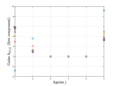
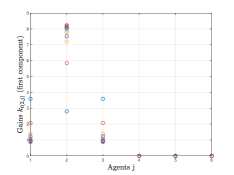
Figure 1: Gain values $k_{t(i,j)}$ (first component) for agents $i=1$ (left) and $i=2$ (right) plotted with respect to $j=1,\ldots,6$.

In Figure 2, we show the evolution of the position error with respect to the desired trajectory $x_{\text{des}_{i}}$ for the two components $(x_{i})_{1}$ and $(x_{i})_{2}$ of all agents $i=1,\ldots,N$.

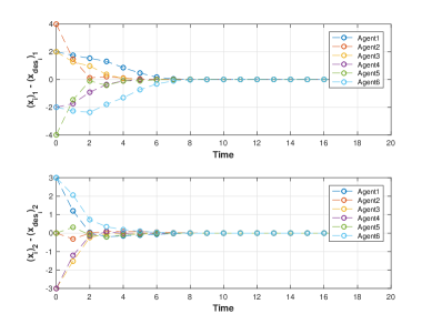
Figure 2: Error with respect to the desired trajectory $x_{\text{des}_{i}}$ for all agents $i=1,\ldots,6$.

VI Conclusions

In this paper we have proposed a fully-distributed strategy to solve nonlinear optimal control problems over networks. The strategy extends the one proposed in our previous work [7] in which a cloud was used together with distributed computation. The main distinctive feature of the new algorithm is the design of a sparse stabilizing controller allowing agents to stabilize system trajectories (at each iteration of the optimal control algorithm) in a distributed way. By relying on polytopic LPV systems, we proposed a two step procedure for the controller design. First, we proposed an iterative algorithm, to be performed offline, to compute “stabilizing” vertex feedback matrices satisfying nonconvex sparsity constraints. Second, we showed how at each iteration nodes can compute feedback gains stabilizing the current trajectory in a fully-distributed way. The controller was tested in simulation on a multi-robot formation control problem.

References

- [1] M. D. Doan, T. Keviczky, and B. De Schutter, “An iterative scheme for distributed model predictive control using Fenchel’s duality,” Journal of Process Control, vol. 21, no. 5, pp. 746–755, 2011.
- [2] P. Giselsson, M. D. Doan, T. Keviczky, B. De Schutter, and A. Rantzer, “Accelerated gradient methods and dual decomposition in distributed model predictive control,” Automatica, vol. 49, no. 3, pp. 829–833, 2013.
- [3] C. Conte, C. N. Jones, M. Morari, and M. N. Zeilinger, “Distributed synthesis and stability of cooperative distributed model predictive control for linear systems,” Automatica, vol. 69, pp. 117–125, 2016.
- [4] D. Groß and O. Stursberg, “A cooperative distributed MPC algorithm with event-based communication and parallel optimization,” IEEE Transactions on Control of Network Systems, vol. 3, no. 3, pp. 275–285, 2016.
- [5] I. Necoara, C. Savorgnan, D. Q. Tran, J. Suykens, and M. Diehl, “Distributed nonlinear optimal control using sequential convex programming and smoothing techniques,” in IEEE Conference on Decision and Control, 2009, pp. 543–548.
- [6] Q. T. Dinh, I. Necoara, and M. Diehl, “A dual decomposition algorithm for separable nonconvex optimization using the penalty function framework,” in IEEE Conference on Decision and Control (CDC), 2013, pp. 2372–2377.
- [7] S. Spedicato and G. Notarstefano, “Cloud-assisted Distributed Nonlinear Optimal Control for Dynamics over Graph,” in IFAC Workshop on Distributed Estimation and Control in Networked Systems, 2018.
- [8] G. Ferrari-Trecate, A. Buffa, and M. Gati, “Analysis of coordination in multi-agent systems through partial difference equations,” IEEE Trans. on Automatic Control, vol. 51, no. 6, pp. 1058–1063, 2006.
- [9] J. Hauser, “A projection operator approach to the optimization of trajectory functionals,” IFAC Proceedings Volumes, vol. 35, no. 1, pp. 377–382, 2002.
- [10] P. Massioni and M. Verhaegen, “Distributed control for identical dynamically coupled systems: A decomposition approach,” IEEE Transactions on Automatic Control, vol. 54, no. 1, pp. 124–135, 2009.
- [11] F. Lin, M. Fardad, and M. R. Jovanović, “Augmented Lagrangian approach to design of structured optimal state feedback gains,” IEEE Trans. on Automatic Control, vol. 56, no. 12, pp. 2923–2929, 2011.
- [12] X. Wu, F. Dörfler, and M. R. Jovanović, “Input-output analysis and decentralized optimal control of inter-area oscillations in power systems,” IEEE Transactions on Power Systems, vol. 31, no. 3, pp. 2434–2444, 2016.
- [13] K. Mårtensson and A. Rantzer, “A scalable method for continuous-time distributed control synthesis,” in American Control Conference (ACC), 2012, pp. 6308–6313.
- [14] B. Polyak, M. Khlebnikov, and P. Shcherbakov, “An LMI approach to structured sparse feedback design in linear control systems,” in European Control Conference, 2013, pp. 833–838.
- [15] A. Jain, A. Chakrabortty, and E. Biyik, “An online structurally constrained LQR design for damping oscillations in power system networks,” in American Control Conference, 2017, pp. 2093–2098.
- [16] M. Farhood, Z. Di, and G. E. Dullerud, “Distributed control of linear time-varying systems interconnected over arbitrary graphs,” Intern. J. of Robust and Nonlinear Control, vol. 25, no. 2, pp. 179–206, 2015.
- [17] M. Farhood, “Distributed control of LPV systems over arbitrary graphs: A parameter-dependent Lyapunov approach,” in American Control Conference, 2015, pp. 1525–1530.
- [18] P. Viccione, C. W. Scherer, and M. Innocenti, “LPV synthesis with integral quadratic constraints for distributed control of interconnected systems,” IFAC Proceedings Volumes, vol. 42, no. 6, pp. 13–18, 2009.
- [19] A. Eichler, C. Hoffmann, and H. Werner, “Robust control of decomposable LPV systems,” Automatica, vol. 50, no. 12, pp. 3239–3245, 2014.
- [20] M. Fardad and M. R. Jovanovic, “On the design of optimal structured and sparse feedback gains via sequential convex programming,” in American Control Conference, 2014, pp. 2426–2431.
- [21] G. Millerioux and J. Daafouz, “Polytopic observer for global synchronization of systems with output measurable nonlinearities,” Intern. Journal of Bifurcation and Chaos, vol. 13, no. 03, pp. 703–712, 2003.
- [22] J. Daafouz and J. Bernussou, “Poly-quadratic stability and H∞ performance for discrete systems with time varying uncertainties,” in IEEE Conference on Decision and Control, vol. 1, 2001, pp. 267–272.
- [23] O. Rozenheck, S. Zhao, and D. Zelazo, “A proportional-integral controller for distance-based formation tracking,” in European Control Conference (ECC), July 2015, pp. 1693–1698.