Singularity formation for rotational gas dynamics

Abstract

The Cauchy problem for the system of equations of two-dimensional rotational gas dynamics is considered. It is assumed that the Cauchy data are a smooth compact perturbation of a constant state. Integral conditions for the data sufficient for the loss of smoothness by a solution within a finite time are found. We analyze the possibility of fulfilling these conditions and compare them with the criterion of singularity formation, known for rotational gas dynamics without pressure.

1 Introduction

We consider a system for density $\varrho({\bf x},t)$, pressure $p({\bf x},t)$, velocity ${\bf u}({\bf x},t)$ and entropy $S({\bf x},t)$:

$$\partial_{t}(\varrho{\bf u})+{\rm div}_{\bf x}({\varrho\bf u}\otimes{\bf u})+\rho l{\mathcal{L}}{\bf u}+\nabla_{\bf x}p = 0,$$ (1)

$$\partial_{t}\varrho+{\rm div}_{\bf x}(\varrho{\bf u}) = 0,$$ (2)

$$\partial_{t}S+{\bf u}\cdot\nabla_{\bf x}S = 0,$$ (3)

$$p=\exp S\varrho^{\gamma}.$$ (4)

Here ${\bf x}\in{\mathbb{R}}^{2},$ $t\geqslant 0$, $\gamma>1$ is the heat ratio, $\mathcal{L}=\left(\begin{array}[]{cr}0&-1\\ 1&0\end{array}\right)$, $l={\rm const}\geqslant 0$ is the Coriolis parameter.

The initial data are the following:

$$({\bf u},\varrho,p)|_{t=0}=({\bf u}_{0},\varrho_{0},p_{0})({\bf x})\in C^{1}({\mathbb{R}}^{2}),$$ (5)

$$\quad(\varrho_{0},p_{0})({\bf x})>0,\quad({\bf u}_{0},\varrho_{0},p_{0})({\bf x})=({\bf 0},\bar{\varrho}_{0},\bar{p}_{0})\,\mbox{for}\,{\bf x}\notin B_{R}(0),$$

$$\bar{\varrho}_{0},\bar{p}_{0}={\rm const}>0,\,B_{R}(0)=\{{\bf x}\big{|}|{\bf x}|<R,\,R={\rm const}>0\}.$$

The system is important because of geophysical applications, since it describes the height-averaged air movement in the atmosphere for middle-scale processes [8]. For $\gamma=2$ the system (1) – (4) corresponds to the equations of rotating shallow water. If $l=0$, then these are the standard hyperbolic compressible Euler equations for polytropic gas; a review of the properties can be found in [1]. System (1) – (4) can be written in a symmetric form, therefore the solution of the Cauchy problem (1) – (5) keep initial smoothness at least for small $t$ [3]. At the same time, the solutions of nonlinear hyperbolic systems have the property of losing smoothness, therefore one of the interesting and difficult problems is to find a class of initial data leading to a blowup in a finite time. In the well-known work [5], integral conditions for the initial data were found that are sufficient for a loss of smoothness. This work has generated many results of this kind for gas dynamics, as well as for systems associated with it, see, for example, [11] and references therein. The results are in some ways simpler for compactly supported solutions [16]. The most elegant theorems regarding energy balance can be obtained for solutions with a finite moment of mass, the pioneering work was [7]. Energy balance and sufficient conditions for a singularity formation for compactly supported solutions of (1) – (4) were obtained in [10], similar results for solution with a finite moment of mass are contained in [11]. Estimates of unavailable potential energy were obtained in [12]. An important result demonstrating that rotation prevents the formation of a singularity can be found in [4], [2].

We note that the issue of the formation of a singularity is very important in the meteorological context since singularities are associated with atmospheric fronts. In addition, knowledge of the class of initial data leading to a blowup helps to study the possibility of the existence of large atmospheric vortices such as typhoons.

Let us introduce the following functionals.

$$G(t)=\frac{1}{2}\int_{B_{R}(t)}|{\bf x}|^{2}\varrho\,dV\geqslant 0,$$

$$F_{1}(t)=\int_{B_{R}(t)}\varrho{\bf u}\cdot{\bf x}\,dV,\quad F_{2}(t)=\int_{B_{R}(t)}\varrho{\bf u}\cdot{\bf x}_{\bot}\,dV,\quad{\bf x}_{\bot}=(x_{2},-x_{1})$$

$$E_{k}(t)=\frac{1}{2}\int_{B_{R}(t)}\varrho|{\bf u}|^{2}\,dV,\quad e(t)=E_{k}(t)+\frac{1}{\gamma-1}\int_{B_{R}(t)}(p-\bar{p})\,dV,$$

$$\quad m(t)=\int_{B_{R}(t)}(\varrho-\bar{\varrho})\,dV,\quad{\bf P}(t)=\int_{B_{R}(t)}\varrho{\bf x}\,dV,\quad{\bf I}(t)=\int_{B_{R}(t)}\varrho{\bf v}\,dV.$$

Such functionals are very convenient for studying various properties of a rotating gas (see [10], [11], [14], [15])

We introduce the notation: $B_{R}(t)=\{{\bf x}\big{|}|{\bf x}|<R+\sigma t\}$, $\sigma=\sqrt{p_{\varrho}}|_{\varrho=\bar{\varrho}}$ is the sound speed (speed of propagation of perturbations).

First of all we note that for $C^{1}$ - smooth solutions of (1) – (5) the support of perturbation is contained in $B_{R}(t)$. It is a corollary of the local energy estimates and can be proved as in [6] for symmetric hyperbolic systems. The rotational term does not give any difference in the prove, since ${\bf u}\cdot{\mathcal{L}}{\bf u}=0$.

Lemma 1.1.

For $C^{1}$ - smooth solutions of (1) – (5) the following properties hold:

$$m^{\prime}(t)=0,$$ (6)

$$e^{\prime}(t)=0,$$ (7)

$$G^{\prime}(t)=F_{1}(t)+\pi\bar{\varrho}\sigma(R+\sigma t)^{3},$$ (8)

$$F_{2}^{\prime}(t)=lF_{1}(t),$$ (9)

$$F_{1}^{\prime}(t)=2E_{k}(t)-2\int_{B_{R}(t)}(p-\bar{p})\,dV-lF_{2}(t),$$ (10)

$${\bf P}^{\prime}(t)={\bf I}(t),$$ (11)

$${\bf I}^{\prime\prime}(t)+l^{2}{\bf I}(t)=0..$$ (12)

Proof.

The proof is a direct calculation of the derivatives of the integrals over the moving volume, taking into account (1), (2) and the Stokes formula.

Corollary 1.

$$lG(t)-F_{2}(t)=lG(0)-F_{2}(0)+\frac{l\pi\bar{\varrho}\sigma}{4}((R+\sigma t)^{4}-R^{4})$$

$$G^{\prime\prime}(t)+l^{2}G(t)=2(2-\gamma)E_{k}(t)+A_{0}+q(t),$$ (13)

$$A_{0}=2(\gamma-1)e(0)+l^{2}G(0)-lF_{2}(0),$$

$$q(t)=\frac{l^{2}\pi\bar{\varrho}}{4}((R+\sigma t)^{4}-R^{4})+3\pi\bar{\varrho}\sigma(R+\sigma t)^{2}.$$

Proof.

The first property follows from (8) and (9). Then together with (10) and (7) we get (13).

2 Inequalities leading to a contradiction

2.1 Lower and upper bounds of $G(t)$

In this section, we obtain general estimates that are independent of $\gamma$.

Lemma 2.1.

For non-trivial $C^{1}$ - smooth solutions of (1) – (5)

$$G(t)>0;$$

$$G(t)\geqslant\phi_{-}(t)\equiv\frac{|{\bf P}(t)|^{2}}{m(0)+\bar{\varrho}\pi(R+\sigma t)^{2}},$$ (14)

where

$$|{\bf P}(t)|^{2}=P^{2}_{1}(t)+P^{2}_{2}(t),\,P_{i}(t)=\int_{0}^{t}I_{i}(\tau)d\tau,i=1,2,$$

$$I_{1}(t)=I_{1}(0)\cos lt+\frac{I_{2}(0)}{l}\sin lt,\quad I_{2}(t)=I_{2}(0)\cos lt+\frac{I_{1}(0)}{l}\sin lt.$$

Proof.

The first statement is evident. To prove the second, we note that from the Hölder inequality we have

$$|{\bf P}(t)|^{2}\leqslant 2G(t)\int_{B_{R}(t)}\varrho\,dV.$$

The explicit form of ${\bf P}(t)$ can be found from (12) and (11). $\square$

Remark 1.

If ${\bf P}(t)=0$ (for example, for axisymmetric initial data), the lower estimate (14) is zero. Otherwise (14) is more exact.

Lemma 2.2.

For non-trivial smooth solutions of (1) – (5)

$$G(t)\leqslant\frac{(R+\sigma t)^{2}}{2}(m(0)+{\bar{\varrho}\pi}(R+\sigma t)^{2})\equiv\phi_{+}(t).$$ (15)

Proof.

The estimate follows from (6) and the inequality

$$G(t)\leqslant\frac{(R+\sigma t)^{2}}{2}\int_{B_{R}(t)}\varrho\,dV.$$

2.2 The case $\gamma=2$, the shallow water equations

In this case equation (13) can be easily solved, namely,

$$G(t)=\frac{1}{4}\sigma^{4}\bar{\varrho}\pi t^{4}+\sigma^{3}\bar{\varrho}\pi Rt^{3}+\frac{3}{2}\sigma^{2}\bar{\varrho}\pi R^{2}t^{2}+\sigma\bar{\varrho}R^{3}t+$$ (16)

$$\frac{F_{1}(0)}{l}\sin lt+(G(0)-\frac{A_{0}}{l^{2}})\cos lt+\frac{A_{0}}{l^{2}}.$$

Thus, if the behavior of $G(t)$ for some $T$ contradicts the upper and lower estimates proved in Sec.2.1,this means that the solution loses smoothness up to this point in time.

We obtain the following result.

Theorem 2.3.

Suppose $\gamma=2$ and there exists a positive $T_{*}$ such that the graphs of functions $G(t)$, given by (16), intersects with $\phi_{-}(t)$, given by (14), or with $\phi_{+}(t)$, given by (15). Then the classical solution of the Cauchy problem (1) – (5) loses smoothness during $T<T_{*}$.

Remark 2.

Since $G(t)$ is the sum of increasing and oscillating functions, it is easy to see that if $T_{*}$ exists, then $T<\frac{2\pi}{l}$ and

$$\left(\frac{A_{0}}{l^{2}}\right)^{2}-\left(\frac{F_{1}^{2}(0)}{l^{2}}+\left(G(0)-\frac{A_{0}}{l^{2}}\right)^{2}\right)\leqslant 0.$$ (17)

However condition (17) is not sufficient for the intersection of graphs of $G(t)$ and $\phi_{-}(t)$.

Remark 3.

Condition (17) holds if and only if

$$-l^{2}G^{2}(0)+2F^{2}_{1}(0)\geqslant 0.$$

It implies that $F_{1}$ (i.e. the radial part of velocity) is initially large enough.

Indeed, (17) implies

$$\frac{8}{l^{4}}e^{2}(0)+(\frac{4}{l^{3}}(2lG(0)-F_{2}(0)))e(t)+\frac{(l^{2}G^{2}(0)-F_{2}(0))^{2}+F^{2}_{1}(0)+F^{2}_{2}(0)}{l^{2}}\leqslant 0,$$ (18)

the left hand side is a quadratic polynomial with respect to $e(0)$. Thus, if the determinant of this polynomial, $-l^{2}G^{2}(0)+2F^{2}_{1}(0)$, is negative, (18) never holds.

2.3 The case $\gamma\neq 2$

In this case we need an additional lemma.

Lemma 2.4.

Assume

$$S_{0}(x)=\ln p_{0}(x)\varrho^{-\gamma}_{0}(x)\geqslant\ln\bar{p}\bar{\varrho}^{-\gamma}\equiv\bar{S},\,x\in{\mathbb{R}}^{2}.$$ (19)

Then

$$\int_{B_{R}(t)}(p-\bar{p})\,dV\geqslant\gamma m(0){\bar{\varrho}}^{\gamma-1}{\exp\bar{S}}=\sigma^{2}m(0).$$

Proof.

Denote $|B_{R}(t)|=\pi(R+\sigma t)^{2}$. First of all, we notice that (3) and (19) imply $S(t,x)\geqslant\bar{S}$ for smooth solutions. Thus,

$$\int_{B_{R}(t)}(p-\bar{p})\,dV=\int_{B_{R}(t)}p\,dV-\bar{p}|B_{R}(t)|=$$

$$\int_{B_{R}(t)}\rho^{\gamma}\exp{S}\,dV-\bar{p}|B_{R}(t)|=\exp{\bar{S}}(\int_{B_{R}(t)}\varrho^{\gamma}\,dV-\bar{\varrho}^{\gamma}|B_{R}(t)|)\geqslant$$

[Jensen’s inequality]

$$\exp{\bar{S}}(|B_{R}(t)|^{1-\gamma}((m(t)+\bar{\varrho}|B_{R}(t)|)^{\gamma}-\bar{\varrho}^{\gamma}|B_{R}(t)|)=$$

$$\exp{\bar{S}}\bar{\varrho}^{\gamma}|B_{R}(t)|\left(\left(\frac{m(t)}{\bar{\varrho}|B_{R}(t)|}+1\right)^{\gamma}-1\right)\geqslant$$

[Bernoulli inequality]

$$\exp{\bar{S}}\bar{\varrho}^{\gamma}|B_{R}(t)|\left(\left(1+\frac{\gamma m(t)}{\bar{\varrho}|B_{R}(t)|}\right)-1\right)=\gamma m(0){\bar{\varrho}}^{\gamma-1}{\exp\bar{S}}.$$

We apply the Bernoulli inequality to obtain

$$\left(\frac{m(t)}{\bar{\varrho}|B_{R}(t)|}+1\right)^{\gamma}\geqslant 1+\frac{\gamma m(t)}{\bar{\varrho}|B_{R}(t)|},$$

since $m(t)+\bar{\varrho}|B_{R}(t)|\geqslant 0$ and therefore $\frac{m(t)}{\bar{\varrho}|B_{R}(t)|}\geqslant-1$. $\square$

Remark 4.

Property (19) always holds for isentropic motion $(S=\rm const)$.

2.3.1 $\gamma>2$

From (13) taking into account the fact that $G(t)$ and $E_{k}(t)$ are nonnegative we have

$$G(t)\leqslant f_{+}(t)\equiv Q(t)+\frac{A_{0}}{2}t^{2}+G^{\prime}(0)t+G(0),$$

$$Q(t)=\int_{0}^{t}\int_{0}^{\tau}q(\lambda)d\lambda d\tau.$$

It is a rough estimate, we can use lower bound (14) to get $-l^{2}G(t)\leqslant-l^{2}\phi_{-}(t).$

Taking into account (15) and Lemma 2.4 from (13) we also have

$$G^{\prime\prime}(t)=-l^{2}G(t)+2e(t)+\frac{2(\gamma-2)}{\gamma-1}\int_{B_{R}(t)}(p-\bar{p})\,dV$$

$$+l^{2}G(0)-lF_{2}(0)+q(t)\geqslant q(t)-l^{2}\psi_{+}(t)+A_{1},$$

$$A_{1}\equiv 2e(0)+l^{2}G(0)-lF_{2}(0)+\frac{2(\gamma-2)}{\gamma-1}\sigma^{2}m(0).$$

Thus,

$$G(t)\geqslant f_{-}(t)\equiv Q_{1}(t)+\frac{A_{1}}{2}t^{2}+G^{\prime}(0)t+G(0),$$

$$Q_{1}(t)\equiv Q(t)=\int_{0}^{t}\int_{0}^{\tau}(q(\lambda)-l^{2}\psi_{+}(\lambda))d\lambda d\tau.$$

Thus, we obtain the theorem.

Theorem 2.5.

Suppose that $\gamma>2$ and condition (19) is satisfied. Assume also that for initial data (5) there exists a positive $T_{*}$ such that the graphs of functions $f_{+}(t)$ and $\phi_{-}(t)$ intersect or the graphs of functions $f_{-}(t)$ and $\phi_{+}(t)$ intersect. Then the classical solution of the Cauchy problem (1) – (5) loses smoothness within a time $T<T_{*}$.

2.4 $\gamma<2$

Analogously to the previous subsection we have from (13)

$$G^{\prime\prime}(t)\geqslant q(t)-l^{2}\psi_{+}(t)+A_{0},$$

$$G^{\prime\prime}(t)=-l^{2}G(t)+2e(t)+\frac{2(\gamma-2)}{\gamma-1}\int_{B_{R}(t)}(p-\bar{p})\,dV$$

$$+l^{2}G(0)-lF_{2}(0)+q(t)\leqslant q(t)+A_{1},$$

$$G(t)\geqslant g_{-}(t)\equiv Q(t)+\frac{A_{1}}{2}t^{2}+G^{\prime}(0)t+G(0),$$

$$G(t)\leqslant g_{+}(t)\equiv Q_{1}(t)+\frac{A_{0}}{2}t^{2}+G^{\prime}(0)t+G(0).$$

Thus, we obtain the theorem.

Theorem 2.6.

Suppose that $\gamma<2$ and condition (19) holds. Assume that for initial data (5) there exists a positive $T_{*}$ such that the graphs of functions $g_{+}(t)$ and $\phi_{-}(t)$ intersect or the graphs of functions $g_{-}(t)$ and $\phi_{+}(t)$ intersect. Then a classical solution to the Cauchy problem (1)-(4), (5) loses smoothness within a time $T<T_{*}$.

Remark 5.

If the time $T_{*}$ from Theorems 2.5 and 2.6 exist, it is sufficiently small.

3 Analysis of sufficient conditions for blowup and examples

In this section we are going to discuss the following questions:

• Can sufficient conditions be satisfied for any data?

• If so, is it possible to judge what kind of singularity arises?

• How rough are the sufficient conditions for the singularity formation? How far are they from the criterion?

• What factors promote or prevent blowup?

1. Let us show that the first question is not trivial. Indeed, we can set for the sake of simplicity $l=0,$ $\bar{\varrho}=\bar{p}=\sigma=0$ and consider axisymmetric initial conditions to have $\phi_{-}=0$. Then for smooth nontrivial solutions we have

$$G^{\prime\prime}(t)=2e(0),\quad G^{\prime}(t)=F_{1}(t),$$

$$e(0)=E_{k}(t)+\int_{B_{R}(t)}p\,dV>E_{k}(t)>0.$$

Thus,

$$G(t)=e(0)t^{2}+G^{\prime}(0)t+G(0),$$ (20)

and $G(t)$ vanishes if and only if

$$(G^{\prime}(0))^{2}\geqslant 4e(0)G(t).$$ (21)

Nevertheless, due to the Hölder inequality $(G^{\prime}(t))^{2}=(F_{1}(t))^{2}\leqslant 4E_{k}(t)G(t)<4e(0)G(t)$. Thus, we get a contradiction with (21) and cannot find the initial data that lead to the blowup. At the same time, it is well known [16] that any solution with compactly supported initial data loses smoothness in a finite time.

This example shows that sufficient conditions for vanishing $G(t)$ do not detect the possible formation of a singularity.

For our simple example, a different method may be proposed. Namely, (20) implies that $G(t)$ is unbounded. However, from (15) we get that in our case $G(t)\leqslant\frac{R^{2}}{2}m(0)\equiv G_{m}$. This contradiction show that any nontrivial solution blowups (in fact, we reproduce the method of proof from [16]).

2. In contrast to the case $l=0$, for $l\neq 0$ sufficient conditions from Theorems 2.3, 2.5, 2.6, not always imply a blowup for compactly supported initial data.

For example, for any $\gamma>1$ we can write

$$G^{\prime\prime}(t)\geqslant 2e(0)-l^{2}(G_{m}-G(0))-lF_{2}(0)\equiv A_{3}.$$

Thus, to obtain a contradiction with the inequality $G(t)\leqslant G_{m}$, we can require, for example, $A_{3}>0$. Nevertheless, since $G_{m}-G(0)>0$, for any initial data we can obtain $A_{3}<0$, increasing $l$.

3. Analysis of sufficient conditions, considered in this paper, show that as $l$ increases, then harder to detect a blowup. Of course this still does not mean that the rotation prevents a blowup. We can draw this conclusion only if there is a criterion for the formation of a singularity (see Example 2 for the case of pressureless gas dynamics). Thus, here we can conclude that increasing rotation we can obtain globally smooth in time solution starting from any smooth initial data.

Further, the absence of axial symmetry also promotes the implementation of sufficient conditions, since a nonzero lower bound $\psi_{-}$ for $G(t)$ arises.

And finally, the lower the speed of sound (that is, the speed of propagation of the support), the simpler the fulfillment of the integral sufficient conditions.

4. From the Hölder inequality we have

$$(F_{1}(t))^{2}=(G^{\prime}(t))\leqslant 4G(t)E_{k}(t),$$ (22)

therefore if $G(t)\to 0$ as $t\to T$, and $F_{1}(T)\neq 0$, then $E_{k}(t)\to\infty$ as $t\to T$. Therefore, provided the solution keeps smoothness up to the time $T$, the density and/or velocity tend to infinity.

5. Inequality (3) also allows to estimate the kinetic energy $E_{k}$ from below. Namely,

$$E_{k}(t)\geqslant\frac{(F_{1}(t))^{2}}{4G(t)}\geqslant\frac{(F_{1}(t))^{2}}{4\psi_{+}(t)}.$$

6. The sufficient conditions considered here help to find perturbations of initial data which are so strong they almost immediately generate a singularity. Indeed, for large $t$ function $G(t)$ increases. However, the growth rate as $t\to\infty$ is slower than the growth rate of its upper boundary $\psi_{+}$ (for the case $\gamma=2$ it is easier to see).

3.1 Example 1

As an example, we consider perturbations of a steady vortex, constructed following to [9] in the isentropic case ($S=\rm const$). Below we set $l=1$.

As the initial data, which are a perturbation of a constant state inside $|{\bf x}|=r\leqslant R=1$ we choose

$${\bf u}_{0}=\frac{\Phi^{\prime}(r)}{r}\left(\begin{array}[]{cr}\epsilon&1\\ -1&\epsilon\end{array}\right)\left(\begin{array}[]{c}x_{1}\\ x_{2}\end{array}\right),$$ (27)

where

$$\Phi=\frac{b}{4}\left\{\begin{array}[]{cr}r^{2}(2-r^{2}),&r\leqslant 1\\ 1,&r>1\end{array}\right.,$$

and

$$p_{0}=(\bar{\Pi}+\Pi)^{\gamma},\quad\varrho_{0}=\left(\frac{p_{0}}{C}\right)^{\frac{1}{\gamma}},$$

where

$$\Pi=\frac{b}{12}\left\{\begin{array}[]{cr}(2br^{4}+3b(1-2b)r^{2}+6(b-1)),&r\leqslant 1\\ 2b-3,&r>1\end{array}\right..$$

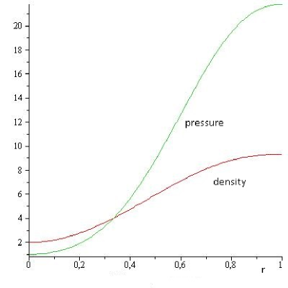
Figure 1: Profiles of density and pressure for a steady state solution (Example 1)

We set $\gamma=2$, so we have an explicit formula for $G(t)$, and choose $C=\frac{1}{4}$, $\bar{\Pi}=1$. The constant $b$ is a measure of vorticity, for our computations we choose $b=-4.$ If $\epsilon=0$, the initial data correspond to a steady state. $\epsilon>0$ corresponds to initially divergent motion, whereas $\epsilon<0$ corresponds to initially convergent one. Fig.1 presents initial profiles of density and pressure as functions of $r$ inside the support of perturbation.

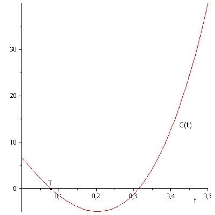
Figure 2: $G(t)$ and $\phi_{-}(t)=0$ for $\epsilon=10$ (left); $G(t)$ and $\phi_{+}(t)$ for $\epsilon=-10$ (right).

Pic.2 shows the intersection of graphs of $G(t)$ and $\phi_{-}=0$ (the data are axisymmetric) for $\epsilon=10$, highly convergent motion (left) and the intersection of graphs of $G(t)$ and $\phi_{+}(t)$ for $\epsilon=-10$, highly divergent motion (right). We can see that the singularity appears very fast.

3.2 Example 2

We study how far the sufficient conditions for the singularity formation are far from the criterion on the example of pressureless gas dynamics, i.e. $C=0$. It seems, that this the only example of multidimensional gas dynamics, where the criterion is known. It was obtained in [4] in Lagrangean formulation and in [13] in Eulerian formulation. In [13] an integral representation of the solution is also obtained. Namely, a solution of (1), (2), $p=0$, keeps smoothness for all $t>0$ if and only if for every point $(x_{1},x_{2})\in{\mathbb{R}}^{2}$

$$({\rm div}\,{\bf u}_{0})^{2}-4\,J({\bf u}_{0})-2\,l\,{\rm rot}\,{\bf u}_{0}-l^{2}<0,$$ (28)

where $J({\bf u}_{0})={\rm det}\big{(}\frac{\partial u_{0i}}{\partial x_{j}}\big{)}$, $i,j=1,2,$ ${\rm rot}{\bf u}_{0}=(u_{02})_{x_{1}}-(u_{01})_{x_{2}}$.

As initial compactly supported velocity ${\bf u}_{0}$ we choose (27) and $\varrho_{0}=1,$ the parameter $l=1$ as before. It can be readily checked by means of (28) that for $\epsilon=0$ the solution to the Cauchy problem for (1)-(2), $p=0$, keeps smoothness for all $t>0$ if $b\in(-0.1,0.2)$ (left and right bounds are approximate). We are going to test the solution with parameter $b=-0.05$. First we perturb the radial component of initial data. Computations show that the solution remain smooth only for $\epsilon\in(-7,2.5)$ If $\epsilon$ does not belong to this domain there are points generating singularity (the bounds are approximate). For $\epsilon>0$ (a divergent motion) these points are close to the boundary of support, for $\epsilon<0$ (a convergent motion) these points are close to the center. The function $G(t)$ obeys the equation

$$G^{\prime\prime}(t)+l^{2}G(t)=2e(0)+l^{2}G(0)-lF_{2}(0)\equiv A_{4},$$

therefore the solution can be found explicitly. It is also easy to find conditions that contradict bilateral inequality $0\leqslant G(t)\leqslant G_{m}.$ The conditions look like (17), namely

$$\left(\frac{A_{0}}{l^{2}}\right)^{2}-\left(\frac{F_{1}^{2}(0)}{l^{2}}+\left(G(0)-\frac{A_{0}}{l^{2}}\right)^{2}\right)\leqslant 0.$$

and

$$\left(G_{m}-\frac{A_{0}}{l^{2}}\right)^{2}-\left(\frac{F_{1}^{2}(0)}{l^{2}}+\left(G(0)-\frac{A_{0}}{l^{2}}\right)^{2}\right)\leqslant 0.$$

Both conditions give approximately the same limitations on $\epsilon$ leading to a blowup, $|\epsilon|>30$. However, we saw that, in fact, the solutions already blow up for $|\epsilon|>7$. Thus, the sufficient conditions for a singularity formation considered here are quite rough and the class of initial data such that the corresponding solution loses smoothness, much broader than that specified in integral sufficient conditions, so they are far from being precise.

References

- [1] G.-Q. Chen, Euler Equations and Related Hyperbolic Conservation Laws, in: Handbook of differential equations: evolutionary equations, Vol.2, Editors: C.M. Dafermos, E. Feireisl, Elsevier: North Holland, 2005.
- [2] B. Cheng and E.Tadmor, Long time existence of smooth solutions for the rapidly rotating shallow-water and Euler equations. SIAM Journal on Mathematical Analysis 39(5) (2008) 1668-1685.
- [3] T.Kato, The Cauchy problem for quasi-linear symmetric hyperbolic systems. Arch. Rational Mech. Anal. 58, 181–205 (1975).
- [4] H.Liu, E.Tadmor, Rotation prevents finite-time breakdown. Physica D: Nonlinear Phenomena, 188(2004) 262–276.
- [5] T.C.Sideris, Formation of singularities in three-dimensional compressible fluids. Comm.Math.Phys. 101(1985). 475–485.
- [6] T.C.Sideris, Formation of singularities in solutions to nonlinear hyperbolic equations. Arch. Rational Mech. Anal. 86, 369–381 (1984).
- [7] J.-Y.Chemin, Dynamique des gaz à masse totale finie, Asymptotic Analysis. 3(1990). 215–220
- [8] J. Pedlosky, Geophysical Fluid Dynamics, Springer-Verlag, Berlin, 1992.
- [9] O.S. Rozanova, Frozen and almost frozen structures in the compressible rotating fluid, Bulletin of the Brazilian Mathematical Society, 47 (2016), N 2, 715–726.
- [10] O.S. Rozanova, Generation of singularities of compactly supported solutions of the Euler equations on a rotating plane, Differential Equations, V.34 (1998), N 8, 1114–1118.
- [11] O.S. Rozanova, Formation of singularities of solutions of the equations of motion of compressible fluids subjected to external forces in the case of several spatial variables, Journal of Mathematical Sciences, 143 (2007), N 4, 3355–3376.
- [12] O.S. Rozanova, Energy balance in a model of the dynamics two-dimensional baroclinic atmosphere, Izvestia of Russuan Academy of Sciences. Physics of Atmosphere and Ocean. 34 (1998), N 2, 189–196.
- [13] O.S. Rozanova, O.I. Uspenskaya, The solution of the Cauchy problem for the two-dimensional transport equation on a rotating plane, to appear in Moscow University Math.Bull. ( ArXiv e-prints, 1909.08502)
- [14] O.S. Rozanova, M.K. Turzynsky, On Systems of Nonlinear ODE Arising in Gas Dynamics: Application to Vortical Motion, Differential and Difference Equations with Applications. Springer Proceedings in Mathematics and Statistics. 230 (2018), 387-398.
- [15] O.S. Rozanova, M.K. Turzynsky, Nonlinear stability of localized and non-localized vortices in rotating compressible media, Theory, Numerics and Applications of Hyperbolic Problems. Springer Proceedings in Mathematics and Statistics. 236 (2018), 567-580.
- [16] Z.-P.Xin, Blowup of smooth solutions to the compressible Navier-Stokes equation with compact density. Comm.Pure Appl.Math. 51(1998), 229–240.