Hyperparameter Optimization for Forecasting Stock Returns

Abstract

In recent years, hyperparameter optimization (HPO) has become an increasingly important issue in the field of machine learning for the development of more accurate forecasting models. In this study, we explore the potential of HPO in modeling stock returns using a deep neural network (DNN). The potential of this approach was evaluated using technical indicators and fundamentals examined based on the effect the regularization of dropouts and batch normalization for all input data. We found that the model using technical indicators and dropout regularization significantly outperforms three other models, showing a positive predictability of 0.53$\%$ in-sample and 1.11$\%$ out-of-sample, thereby indicating the possibility of beating the historical average. We also demonstrate the stability of the model in terms of the changes in its feature importance over time.

1 Introduction

Deep learning has become a promising way to model the complexity of stock movements. It enables us to capture non-linear movements, to associate large data, and to reduce noise without an assumption of a pre-specified underlying structure. At the same time, it leaves us with a difficulty in selecting numerous hyperparameters, which critically affects the performance of the resulting models. Most studies dealing with a financial time series typically choose pre-specified hyperparameters and check the robustness of the model based on small changes in the parameters. This approach requires experts to put a lot of effort into tuning numerous parameters simultaneously, which often results in a suboptimal model.

Hyperparameter optimization (HPO) can be used to mitigate this problem by automatically searching for the most optimal hyperparameters in machine learning learners, and has been widely used to identify good configurations more quickly, such as through the use of a sequential model-based algorithm configuration (SMAC), tree-structure Parzen estimator (TPE), and Sprearmint [1]. HPO has also been demonstrated to be an extremely powerful approach for automatic image and speech recognition, and offers advantages for dealing with machine learning in a systematic manner. First, it reduces the human effort necessary in tuning the hyperparameters and opens up the possibility of improving the performance of machine learning [2][3]. Second, it improves the reproducibility and fairness of scientific studies because an automated HPO is more reproducible than a hand-tuned approach using trial-and-error searches to produce a desired behavior, thereby allowing us to compare different methods more fairly through the same level of tuning [4][5].

Despite such advantages, financial studies have generally not considered this method. HPO requires a large data scale to avoid an overfitting occurring in both the training and validation data. Stock-related data are obtained only over a relatively short time span, typically from the year 1950 to the present. As shown in Fig. 1, a random evolution of a stock return, such as time-varying volatility and occasional jumps related to crashes or sudden upsurges, causes a time dependency of the model parameter set to specific periods. Furthermore, cross-validation and shuffling, which are crucial techniques for preventing an overfitting, cannot be used because stock-related data are time-ordered, and a modeling process requires preserving the time ordering. For these reasons, the use of HPO has rarely been assessed and there is a poor understanding of its efficiency in financial data modeling. As a result, practitioners need to pay more attention to hyperparameter tuning and the resulting models largely depending on their experience.

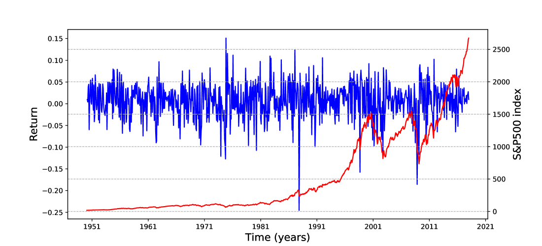
Figure 1: S$\&$P 500 index and its returns from Jan. 1, 1950 to Dec. 31, 2017.

In this study, we evaluate the viability of HPO in terms of the stock return predictability problem. We examined the HPO performance across different conditions, the input features of the fundamentals and technical indicators, and the regularization of a dropout and batch normalization. Our key findings are as follows:

• We show that, whereas the prediction models with an input of fundamentals are likely to overfit the in-sample data, models with the input feature of the technical indicators achieves a strong predictability throughout the in- and out-of-sample periods. A dropout is more effective for a positive predictability in an out-of-sample than a batch normalization.

• We show that the model with good predictability in both an in- and out-of-sample is less sensitive to the time evolution, which reveals that it is a general model for adapting to the changes in the economic and business conditions.

We believe this study provides insight into the application of machine learning for investment purposes or risk management.

Related work In financial economics, there is a long-standing debate whether (excess) stock market returns are predictable. The conventional framework for analyzing equity premium predictability is a ‘linear predictive regression’ model taking the following form:

$$r_{t+1}=\alpha+\bm{\beta}^{{}^{\prime}}\bm{x}_{t}+\varepsilon_{t+1},$$ (1)

where $r_{t+1}$ is the return on the stock market index in excess of the risk-free interest rate, $\alpha$ is an intercept term, $\bm{\beta}$ is a $p\times 1$ dimensional vector of the slope parameters, $\bm{x}_{t}$ is a $p\times 1$ dimensional vector of the predictor variables observed at time $t$, and $\varepsilon_{t+1}$ is a zero-mean disturbance term. The most commonly followed approaches are the use of individual bivariate regressions using one variable at a time from the Goyal and Welch (GW) predictor variables [6], or a multivariate regression, which includes the full set of GW predictors in (1) (see [7][6][8] for a bivariate regression and [9][10][11] for a multivariate regression).

Deep learning models are on the rise, showing impressive results in modeling the complex behavior of financial data. Examples include stock prediction based on long short-term memory (LSTM) networks [12], deep portfolios based on deep autoencoders [13], threshold-based approaches using recurrent neural networks [14], and deep factor models involving deep feed-forward networks [15], LSTM networks [16], and fundamentals [17]. These studies apply hand-tuned hyper-parameters.

In section 2, we provide the data used in this study and the preprocessing methods. In section 3, we describe the experimental setting and its implementation. In section 4, we provide the experimental results and make comparisons between models. Finally, some concluding remarks are given in section 5.

2 Data and preprocessing

We used sets of fundamentals and technical indicators that have traditionally been used for studying stock predictability.

Technical indicators Technical analysis is a method for forecasting price movements using past prices and volume and includes a variety of forecasting techniques such as a chart analysis, cycle analysis, and computerized technical trading systems.

Technical analysis has a long history of widespread use by participants in speculative markets [18] [19] [20] [21] [22] [23], and there is a large body of academic evidence demonstrating the usefulness of a technical analysis, including theoretical support [24] and empirical evidence [25][26], as well as their role in out-of-sample equity premium predictability [27] [9] [10].

The monthly market data for the S$\&$P500 were obtained from Yahoo Finance and contain daily trading data, i.e., the opening prices, high prices, low prices, adjusted closing prices, and end-of-day volumes. The data are from the period between January 1, 1950 and December 31, 2017 (Fig. 1). We used a full set of 14 technical indicators based on 3 types of popular technical strategies, moving average crossover rules, momentum rules, and volume rules:

• The time-series momentum indicator, MOM($m$), is the generation of a buy signal when the price is higher than the historical price. Its validation is supported by the observation that the “trend” effect persists for approximately 1 year and then partially reverses over a longer timeframe. Here, $\textrm{MOM}_{t}(m)$ at time $t$ is defined as follows:

  $$\textrm{MOM}_{t}(m)=\begin{cases}1\textrm{ (Buy signal) },&\text{if}\quad P_{t}\geq P_{t-m}\\ -1\textrm{ (Sell signal) },&\text{otherwise}.\end{cases}$$ (2)

  where $P_{t}$ is the index value at time $t$, and $m$ is the look-back period. We use $m=1,3,6,9$ and $12$, which are respectively labeled as $\textrm{MOM}_{t}$(1M), $\textrm{MOM}_{t}$(3M), $\textrm{MOM}_{t}$(6M), $\textrm{MOM}_{t}$(9M), and $\textrm{MOM}_{t}$(12M).

• The moving average indicator, MA$(s,l)$, provides a signal for an upward or downward trend. A buy signal is generated when the short-term moving average crosses above the long-term moving average because this represents the beginning of an upward trend. A sell signal is generated when the short-term moving average crosses below the long-term moving average because this represents the beginning of a downward trend.

  Let us define a simple moving average of the index as follows:

  $$\textrm{MA}_{j,t}^{P}=(1/j)\sum_{i=0}^{j-1}P_{t-m}\textrm{ for }j=s\textrm{ or }l,$$ (3)

  where $s$ and $l$ are the look-back periods for short and long moving averages. The moving average indicator $\textrm{MA}_{t}(s,l)$ is then designed as follows:

  $$\textrm{MA}_{t}(s,l)=\begin{cases}1\textrm{ (Buy signal) },&\text{if}\quad\textrm{MA}_{s,t}^{P}\geq\textrm{MA}_{l,t}^{P}\\ -1\textrm{ (Sell signal) },&\text{otherwise}.\end{cases}$$ (4)

  The six moving average indicators are constructed for $s=1$, $2$, $3$, and $l=9$, $12$, which are symbolized as MA(1M-9M), MA(1M-12M), MA(2M-9M), MA(2M-12M), MA(3M-9M), and MA(3M-12M).

• The volume indicator, VOL($s,l$), indicates a strong market trend if the recent stock market volume and stock price increase. Let us define the on-balance volume (OBV) as follows:

  $$\textrm{OBV}_{t}=\sum_{k=1}^{t}VOL_{k}D_{k},$$ (5)

  where $VOL_{k}$ is a measure of the trading volume (i.e., number of shares traded) during period $k$, and $D_{k}$ is a binary variable:

  $$D_{k}=\begin{cases}1,&\text{if}\quad P_{k}\geq P_{k-1}\\ -1,&\text{otherwise}.\end{cases}$$ (6)

  The value of $\textrm{OBV}_{t}$ conceptionally measures both positive and negative volume based on the belief that changes in volume can predict a stock movement. The volume-based indicator is then defined as the difference between the moving averages with a $s$-period and $l$-period:

  $$\textrm{VOL}(s,l)=\begin{cases}1\textrm{ (Buy signal) },&\text{if}\quad\textrm{MA}_{s,t}^{\textrm{OBV}}\geq\textrm{MA}_{l,t}^{\textrm{OBV}}\\ -1\textrm{ (Sell signal) },&\text{otherwise}.\end{cases}$$ (7)

  Here, $\textrm{MA}_{j,t}^{\textrm{OBV}}=(1/j)\sum_{i=0}^{j-1}\textrm{OBV}_{t-i}$ is the moving average of $\textrm{OBV}_{t}$ for $j=s$ or $l$. The six moving average indicators are constructed for $s=1$, $2$, $3$ and $l=9$, $12$, which are symbolized as VOL(1M-9M), VOL(1M-12M), VOL(2M-9M), VOL(1M-12M), VOL(3M-9M) and VOL(3M-12M).

Fundamental indicators We use the financial indicators employed by [6] for the U.S. stock market, which is available from Amit Goyal’s web site. We use updated data consisting of 14 popular fundamental variables spanning from January 1950 to December 2017. We provide a short definition of these variables as follows.

• Dividend-price ratio, DP: Log of a 12-month moving sum of dividends paid on the S&P 500 index minus the log of the stock prices.

• Dividend yield, DY: Log of a 12-month moving sum of dividends minus the log of 1-month lagging stock prices.

• Earning-price ratio, EP: Log of a 12-month moving sum of earnings on the S&P 500 index minus the log of the stock prices.

• Dividend-payout ratio, DE: Log of a 12-month moving sum of dividends minus the log of a 12-month moving sum of earnings.

• Stock variance, SVAR: Sum of squared daily returns on the S$\&$P500.

• Book-to-market ratio, BM: Ratio of book value to market value for the Dow Jones Industrial Average.

• Net equity expansion, NTIS: Ratio of 12-month moving sum of net issues by NYSE listed stocks divided by their total market capitalization.

• Treasury Bill rate, TBL: Interest rate on a 3-month treasury bill from the secondary market.

• Long-term yield, LTY: Long-term government bond yields.

• Long-term rate of return, LTR: Long-term government bond returns

• Term spread, TMS: Difference between the long and term yield on government bonds and T-bills.

• Default yield spread, DFY: Difference between BAA- and AAA-rated corporate bonds and returns on long-term government bonds.

• Default return spread, DFR: Difference between the return on long-term corporate bonds and returns on the long-term government bonds.

• Inflation, INFL: Consumer Price Index (CPI) for all urban consumers.
  

3 Experiments

Data Splits: As mentioned earlier, the predictability found in traditional studies is not uniform over time and is concentrated within certain periods [10]. To check the robustness, we investigated the predictability over four different periods, the entire period of $1950-2017$ (Exp. 1) and its sub-periods of $1950-2015$ (Exp. 2), $1950-2007$ (Exp. 3), and $1950-2002$ (Exp. 4). For each experiment, we split the data into in-sample and out-of-sample periods. The in-sample data were divided into a training dataset (50$\%$) for developing the prediction models and a validation set (50$\%$) for evaluating its predictive ability.

Training: Deep feedforward neural networks (DNNs) were used in this study. We applied TPE for automated hyperparameter tuning with additional tests using simulated annealing and a random search to further confirm our results. The hyperparameters and their prior distributions are summarized in Table 1. For hyperparameter selection, we trained DNNs on an in-sample training set and selected the model with the lowest validation error. We limited the number of function evaluations for finding optimal hyper-parameters to $50$. Each evaluation comprised training the DNN models for 200 epochs and selecting the model with the lowest validation error.

Regularizer: We are particularly interested in regularization methods for model generalization because the time-dependent behavior of financial data is likely to cause a parameter instability over an out-of-sample. We examined the effectiveness of the most popular regularization methods, namely, a dropout and batch normalization (BN). A dropout[28] is a simple way to prevent co-adaptation among hidden nodes of deep feed-forward neural networks by randomly dropping out selected hidden nodes. In recent years, batch normalization [29] has replaced a dropout in modern neural network architectures. It uses the distribution of the summed input to a neuron over a mini-batch of training cases to compute the mean and variance, which are then used to normalize the summed input to the neuron for each training case. Dropout and BN layers are employed for all hidden layers.

Table 1: List of parameters and their corresponding range of values used in the grid search.

Hyperparamter		Considered values/functions
Number of Hidden Layers		{2, 3}
Number of Hidden Units		{2, 4, 8, 16}
Standard deviation		{0.025,0.05,0.075}
Dropout		{0.25, 0.5, 0.75}
Batch Size		{28, 64, 128}
Optimizer		{RMSProp, ADAM, SGD (no momentum)}
Activation Function		Hidden layer: {tanh, ReLU, sigmoid}, Output layer: Linear
Learning Rate		{0.001}
Number of Epochs		{100}

Number of Layers: number of the layers of the neural network. Number of Hidden Units: number of units in the hidden layers of the neural network. Standard Deviation: standard deviation of a random normal initializer. Dropout: dropout rates. Batch Size: number of samples per batch. Activation: sigmoid function $\sigma(z)=1/(1+e^{-z})$, hyperbolic tangent function $\textrm{tanh}(z)=(e^{z}-e^{-z})/(e^{z}-e^{-z})$, and rectified linear unit (ReLU) function $\textrm{ReLU}(z)=\textrm{max}(0,z)$. Learning Rate: learning rate of the back-propagation algorithm. Number of Epochs: number of iterations for all of the training data. Optimizer: stochastic gradient descent (SGD) [30], RMSProp [31], and ADAM [30]

Out-of-sample $R^{2}$ statistic: We measured the out-of-sample $R^{2}$ statistics ($R_{\textrm{OS}}$) [8] for a comparison with the in-sample $R^{2}$ statistics ($R^{2}_{\textrm{IS}}$) and evaluated the forecasting power of the models. The $R_{\textrm{OS}}^{2}$ statistic measures the improvement in the mean square forecast error (MSFE) for the return forecast relative to the simple historical average (or constant expected return) forecast, which ignores information contained in the predictors. This is computed as follows:

$$R^{2}_{\textrm{OS}}=1-\frac{\sum_{t=1}^{T}(r_{t}-\hat{r}_{t})^{2}}{\sum_{t=1}^{T}(r_{t}-\bar{r}_{t})^{2}},$$ (8)

where $\hat{r}_{t}$ is the fitted value from a predictive regression estimated through period $t-1$, and $\bar{r}_{t}$ is the historical average return estimated through period $t-1$.

Model stability: We analyzed the model stability over time in terms of the feature importance. Stock price dynamics is so complex with complicated interactions among changing micro behavior, varying product cycles, interdependent industrial structures, and cyclic macro environment, thus it leads to gradual or sudden shifts in the model parameters. For example, traditional univariate models are highly exposed to the model instability in the in-sample, which demonstrates the time-dependency of the statistical significance and the coefficient of the predictor variables [10]. To overcome this problem, a multivariate regression model is proposed through which the changes to the parameters at breaks are estimated [32].

We examined the stability of the trained model over time by computing the SHapley Additive exPlanation (SHAP) values of the features [33] to find the contribution of the features in the prediction and determine the change in ranking of the features over time.

4 Results

4.1 Technical Indicators

4.1.1 Dropout versus batch normalization

We compared a DNN with a dropout and a DNN with batch normalization for the four experiments. The following observations can be made regarding the results reported in Table 4.1.1.

• Both DNNs show a good in-sample predictive power of a positive $R^{2}_{\textrm{IS}}$ for all experiments. The in-sample predictive power of the BN ranging over 1.740 to 2.968 is stronger than that of the dropout ranging over 0.424 to 0.748.

• The DNN with a dropout achieves a good out-of-sample predictive power, showing positive $R^{2}_{OS}$ values for all experiments, which means that it outperforms the historical mean return over the training and validation periods. However, the BM model achieves a poor out-of-sample predictive power, with negative $R^{2}_{OS}$ values for all experiments. A dropout is more effective at preventing a model instability.

• The instability of the BN model is derived from an overfitting to the in-sample set based on the observation that, although $\textrm{MSE}_{\textrm{train}}$ and $\textrm{MSE}_{\textrm{val}}$ of the BN model are lower than those of the dropout model (except for only $\textrm{MSE}_{\textrm{train}}$ in Exp. 2), $\textrm{MSE}_{\textrm{test}}$ of the BN model is higher than that of the dropout model. Figure 2 graphically shows the overfitting occurring during the training in Exp. 1.

• The results indicate that an in-sample predictive content does not necessarily translate into an out-of-sample predictive ability, nor ensure the stability of the predictive relation over time.

• The degree of predictability varies according to the experimental period, showing that Exp. 2 and 3 show a strong predictability of $1.889$ and $1.670$, and Exp. 1 and 4 show a relatively weak predictability of $0.569$ and $0.319$, respectively.

• Figure 3 graphically shows how to beat the historical average in Exp. 1. The dropout model forecasts returns around the mean of the out-of-sample, whereas the historical average showed a greater deviation. This means the model can be adjusted better to a new market environment than the historical average.

• The DNN with a dropout achieves an average predictability of 0.53$\%$ in-sample and 1.11$\%$ out-of-sample. The DNN with a dropout has an average predictability of 2.312$\%$ in-sample and $-2.8545\%$ out-of-sample.

Table 2: Comparison of models based on average prediction performance ($\pm$1 s.d. in parentheses) over 5 runnings with different random initial seeds for each experiment.

Model	$\textrm{MSE}_{\textrm{train}}$	$\textrm{MSE}_{\textrm{val}}$	$\textrm{MSE}_{\textrm{test}}$	$R^{2}_{IS}$	$R^{2}_{OS}$
	Exp. 1
DNN w. dropout	0.129 ($\pm 3.236$)	0.197 ($\pm 0.171$)	$\bm{0.186}$ ($\pm\bm{1.506}$)	0.748 ($\pm$1.040)	$\bm{0.569}$ ($\bm{\pm 0.621}$)
DNN w. BN	$\bm{0.128}$ ($\bm{\pm 0.646}$)	$\bm{0.193}$ ($\bm{\pm 1.333}$)	0.194 ($\pm 1.713$)	$\bm{1.740}$ (	$-3.74$ ($\pm$0.804)
	Exp. 2
DNN w. dropout	$\bm{0.126}$ ($\bm{\pm 0.062}$)	0.206 ($\pm 0.130$)	$\bm{0.201}$ ($\bm{\pm 0.540}$)	0.451 ($\pm$0.028)	$\bm{1.889}$ ($\bm{\pm 0.242)}$
DNN w. BN	0.127 ($\pm 1.739$)	$\bm{0.201}$ ($\bm{\pm 0.298}$)	0.209 ($\pm 3.240$)	$\bm{1.890}$ ($\bm{\pm 0.293}$)	$-2.70$ ($\pm$0.906)
	Exp. 3
DNN w. dropout	0.130 ($\pm 0.189$)	0.216 ($\pm 0.038$)	$\bm{0.147}$ ($\bm{\pm 0.174}$)	0.507 ($\pm$0.056)	$\bm{1.670}$ ($\bm{\pm 0.143}$)
DNN w. BN	$\bm{0.125}$ ($\bm{\pm 1.618}$)	$\bm{0.213}$ ($\bm{\pm 0.768}$)	0.153 ($\pm 2.781$)	$\bm{2.650}$ ($\bm{\pm 0.543}$)	$-3.518$ ($\pm$2.650)
	Exp. 4
DNN w. dropout	0.1193 ($\pm 0.697$)	0.197 ($\pm 0.716$)	$\bm{0.218}$ ($\bm{\pm 0.356}$)	0.424 ($\pm$0.181)	$\bm{0.319}$ ($\bm{\pm 0.139}$)
DNN w. BN	$\bm{0.115}$ ($\bm{\pm 3.998}$)	$\bm{0.196}$ ($\bm{\pm 0.702}$)	0.219 ($\pm 2.160$)	$\bm{2.968}$ ($\bm{\pm 0.959}$)	$-1.460$ ($\pm$0.989)

• Note: All the MSE and $R^{2}$ values have been multiplied by a factor of $10^{-2}$ and all the s.d. values has been multiplied by a factor of $10^{-5}$.

Figure 2: Validation and testing errors of the DNNs with dropout and with BN with regards to $50$ function evaluations and 200 epochs for each function evaluation. The (dashed) lines are the average score over five random initializations and the shaded regions correspond to one standard deviation.

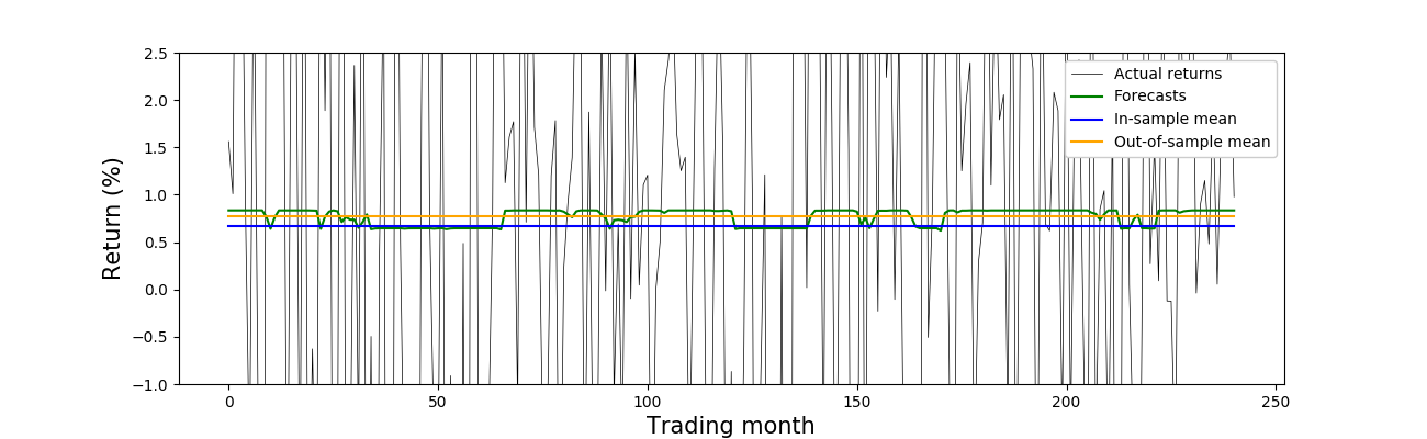
Figure 3: Comparison of actual and predicted values over the out-of-sample period. The actual return is drawn by the thin solid black line. Forecasted values from the DNN with dropout, in-sample mean, and out-of-sample mean are drawn by the solid green, blue and yellow lines, respectively.

4.1.2 Effect of optimizer choice

To further check the robustness of a dropout with respect to the dependency on the selected optimization algorithm, we repeated the experiments using a random search and simulated annealing. As shown in Fig. 4, a comparable performance is shown for both the validation and test set, without an overfitting to the former. Our observations on different optimizers consistently suggest that a dropout helps improve the generalization. This indicates that the benefits of the HPO are general, without depending on a specific optimizer, thereby demonstrating its robustness.

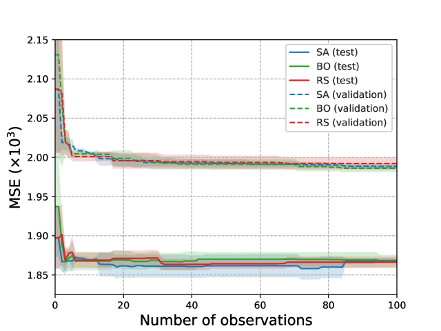
Figure 4: Comparison of the simulated annealing (SA), TPE, and random search (RS) performances on the validation and test sets for the first 100 observations. The (dashed) lines are the average score over five random initializations and the shaded regions correspond to one standard deviation.

4.1.3 Model stability over time

Figure 4.1.1 shows the importance of features arranged in decreasing order for the dropout and batch normalization models. They were calculated by summing the absolute values of the SHAP values. Table 3 shows the rank of the features over time from Exp. 4 to Exp. 1. The following observation was made based on the results.

• The feature importance is sensitive to the selected experimental periods for both models. This implies that the selection of a small number of features based on their importance can prevent a model generalization for unseen (new) data.

• Overall, we observed that a DNN with a BN achieves a greater variability than a DNN with a dropout. In the experiments with a dropout, the five variables $\{$MA112, MA212, MA39, MA29, MOM6M$\}$ and the six variables $\{$MOM12M, VOL29, VOL212, VOL312, MOM3M, MOM1M $\}$ remain in the top half (from 1st to 8th) and bottom half across the experiments, respectively. By contrast, in the experiments using a BN, only $\{$MA19$\}$ remains in the top half and $\{$MA29, MA312$\}$ remain in the bottom half. This indicates that a DNN with a dropout is more generalized against a time change and explains the outperformance of $R^{2}_{OS}$ in a more fundamental manner.

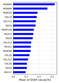
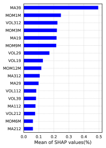
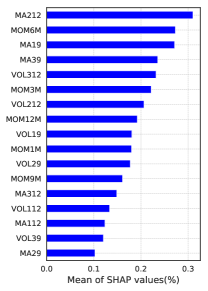
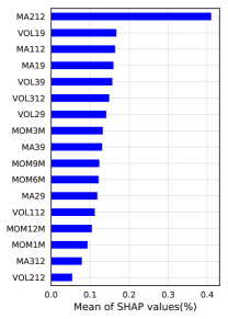
(b) DNN with BN. From left, Exp. 1–4.

Figure 5: Mean absolute value of SHAP values for each features for Exp. 1–4.

Table 3: Feature ranking results of DNNs with dropout (left) and with BN (right).

	Exp. 4	Exp. 3	Exp. 2	Exp. 1
MA112	1	4	3	2
MA212	2	3	4	7
MA39	3	6	5	1
MA19	4	1	1	10
MA29	5	2	2	4
MOM6M	6	5	6	5
VOL19	7	8	8	13
MOM9M	8	9	9	9
MOM12M	9	13	11	11
VOL29	10	10	10	16
VOL212	11	12	14	17
VOL312	12	11	13	12
MA312	13	7	7	14
VOL112	14	14	15	8
VOL39	15	16	16	3
MOM3M	16	15	12	16
MOM1M	17	17	17	15

	Exp. 4	Exp. 3	Exp. 2	Exp. 1
MA212	1	1	17	8
VOL19	2	9	8	4
MA112	3	15	14	17
MA19	4	3	5	6
VOL39	5	16	13	15
VOL312	6	5	3	14
VOL29	7	11	7	13
MOM3M	8	6	4	12
MA39	9	4	1	9
MOM9M	10	12	6	2
MOM6M	11	2	16	1
MA29	12	17	11	16
VOL112	13	14	12	5
MOM12M	14	8	9	7
MOM1M	15	10	2	3
MA312	16	13	10	11
VOL212	17	7	15	10

4.2 Fundamentals

4.2.1 Predictability and model stability

Table 4.2.1 shows the results produced through the same procedure as used in the previous experiments applying fundamentals. The following observations can be made regarding the results.

• For both models, fundamental data are prone to an overfitting to the in-sample data as shown in the positive $R_{IS}^{2}$ and negative $R_{OS}^{2}$ values.

• A DNN with a dropout outperforms a DNN with a BN in terms of better values of $R_{IS}^{2}$ and $R_{OS}^{2}$ except for only $R_{IS}^{2}$ in Exp. 1.

Table 4: Comparison of models based on average prediction performance ($\pm$1 s.d. in parentheses) over 5 runnings with different random initial seeds for each experiment.

Regularizer	$\textrm{MSE}_{\textrm{train}}$	$\textrm{MSE}_{\textrm{val}}$	$\textrm{MSE}_{\textrm{test}}$	$R^{2}_{IS}$	$R^{2}_{OS}$
	Exp. 1
DNN w. dropout	0.129 ($\pm 0.580$)	0.198 ($\pm 0.329$)	$\bm{0.189}$ ($\pm\bm{0.904}$)	$-0.179$ ($\pm$0.177)	$\bm{-0.341}$ ($\bm{\pm 0.620}$)
DNN w. BN	$\bm{0.127}$ ($\bm{\pm 2.778}$)	$\bm{0.193}$ ($\bm{\pm 2.412}$)	0.205 ($\pm 18.817$)	$\bm{2.700}$ (	$-10.462$ ($\pm$9.105)
	Exp. 2
DNN w. dropout	$\bm{0.119}$ ($\bm{\pm 1.797}$)	0.202 ($\pm 0.687$)	$2.334$ ($\pm 15.298$)	$\bm{3.841}$ ($\bm{\pm 0.645}$)	$\bm{-13.794}$ ($\bm{\pm 7.457)}$
DNN w. BN	0.156 ($\pm 9.133$)	$\bm{0.196}$ ($\bm{\pm 0.823}$)	$\bm{0.598}$ (	$-5.098$ ($\pm 2.558$)	$-191.78$ ($\pm$43.838)
	Exp. 3
DNN w. dropout	$\bm{0.122}$ ($\bm{\pm 2.632}$)	2.122 ($\pm 1.185$)	$\bm{0.170}$ ($\bm{\pm 5.285}$)	$\bm{4.248}$ ($\bm{\pm 0.736}$)	$\bm{-13.670}$ ($\bm{\pm 3.527}$)
DNN w. BN	$0.138$ ($\pm 18.870$)	$\bm{0.206}$ ($\bm{\pm 0.715}$)	0.271 ($\pm 134.062$)	$1.160$ ($\pm 5.526$)	$-81.173$ ($\pm$89.469)
	Exp. 4
DNN w. dropout	$\bm{0.113}$ ($\bm{\pm 1.315}$)	0.194 ($\pm 1.385$)	$\bm{0.232}$ ($\bm{\pm 8.753}$)	$\bm{3.443}$ ($\bm{\pm 0.764}$)	$\bm{-6.058}$ ($\bm{\pm 3.992}$)
DNN w. BN	$0.129$ ($\pm 5.911$)	$\bm{0.185}$ ($\bm{\pm 0.121}$)	0.395 ($\pm 49.916$)	$1.003$ ($\pm 1.816$)	$-80.260$ ($\pm$22.767)

• Note: All the MSE and $R^{2}$ values have been multiplied by a factor of $10^{-2}$ and all the s.d. values has been multiplied by a factor of $10^{-5}$.

5 Conclusion

In this study, we explored hyperparameter optimization techniques used in A stock return prediction by applying DNN-based predictors. The experiment was validated by considering different settings for the datasets, periods, and regularization. We found that technical indicators are robust to an overfitting during the HPO procedure, showing positive $R_{IS}$ and $R_{OS}$ values over different time periods, whereas the fundamental indicators are prone to an overfitting to the in-sample data. To summarize, dropout layers can efficiently decrease the risk of an overfitting and increase the model generalizability.

This system can be seen as a first step toward a better and more fruitful integration of the recent developments in HPO techniques. Future efforts for improving the current solution will be devoted to the design of a neural architecture for the fundamental data, which are robust to an overfitting. Fundamental data evidently reflect the fundamental values, which can serve as useful predictors or provide complementary information for a stock return prediction. We expect the development to improve the prediction accuracy by combining fundamental and technical indicators.

References

- [1] Matthias Feurer, Jost Tobias Springenberg, and Frank Hutter. Using meta-learning to initialize bayesian optimization of hyperparameters. In Proceedings of the 2014 International Conference on Meta-learning and Algorithm Selection-Volume 1201, pages 3–10. Citeseer, 2014.
- [2] Gábor Melis, Chris Dyer, and Phil Blunsom. On the state of the art of evaluation in neural language models. In ICLR, Proceedings of the International Conference on Learning Representations, 2018.
- [3] Jasper Snoek, Hugo Larochelle, and Ryan P Adams. Practical bayesian optimization of machine learning algorithms. In Advances in neural information processing systems, pages 2951–2959, 2012.
- [4] James Bergstra, Daniel Yamins, and David Daniel Cox. Making a science of model search: Hyperparameter optimization in hundreds of dimensions for vision architectures. 2013.
- [5] D Sculley, Jasper Snoek, Alex Wiltschko, and Ali Rahimi. Winner’s curse? on pace, progress, and empirical rigor. 2018.
- [6] Ivo Welch and Amit Goyal. A comprehensive look at the empirical performance of equity premium prediction. The Review of Financial Studies, 21(4):1455–1508, 2007.
- [7] Amit Goyal and Ivo Welch. Predicting the equity premium with dividend ratios. Management Science, 49(5):639–654, 2003.
- [8] John Y Campbell and Samuel B Thompson. Predicting excess stock returns out of sample: Can anything beat the historical average? The Review of Financial Studies, 21(4):1509–1531, 2007.
- [9] David E Rapach, Jack K Strauss, and Guofu Zhou. Out-of-sample equity premium prediction: Combination forecasts and links to the real economy. The Review of Financial Studies, 23(2):821–862, 2010.
- [10] Christopher J Neely, David E Rapach, Jun Tu, and Guofu Zhou. Forecasting the equity risk premium: the role of technical indicators. Management science, 60(7):1772–1791, 2014.
- [11] Daniel Buncic and Martin Tischhauser. Macroeconomic factors and equity premium predictability. International review of economics & finance, 51:621–644, 2017.
- [12] Thomas Fischer and Christopher Krauss. Deep learning with long short-term memory networks for financial market predictions. European Journal of Operational Research, 270(2):654–669, 2018.
- [13] JB Heaton, NG Polson, and Jan Hendrik Witte. Deep learning for finance: deep portfolios. Applied Stochastic Models in Business and Industry, 33(1):3–12, 2017.
- [14] Sang Il Lee and Seong Joon Yoo. Threshold-based portfolio: the role of the threshold and its applications. The Journal of Supercomputing, pages 1–18, 2018.
- [15] Kei Nakagawa, Takumi Uchida, and Tomohisa Aoshima. Deep factor model. In ECML PKDD 2018 Workshops, pages 37–50. Springer, 2018.
- [16] Kei Nakagawa, Tomoki Ito, Masaya Abe, and Kiyoshi Izumi. Deep recurrent factor model: Interpretable non-linear and time-varying multi-factor model. arXiv preprint arXiv:1901.11493, 2019.
- [17] John Alberg and Zachary C Lipton. Improving factor-based quantitative investing by forecasting company fundamentals. arXiv preprint arXiv:1711.04837, 2017.
- [18] Seymour Smidt. Amateur Speulators: A Survey of Trading Styles, Information Sources and Patterns of Entry Into and Exit from Commodity-futures Markets by Non-professional Speculators. Graduate School of Business and Public Administration, Cornell University, 1965.
- [19] Randall S Billingsley and Don M Chance. Benefits and limitations of diversification among commodity trading advisors. Journal of Portfolio Management, 23(1):65, 1996.
- [20] William Fung and David A Hsieh. The information content of performance track records: investment style and survivorship bias in the historical returns of commodity trading advisors. Journal of Portfolio Management, 24(1):30–41, 1997.
- [21] Lukas Menkhoff. Examining the use of technical currency analysis. International Journal of Finance & Economics, 2(4):307–318, 1997.
- [22] Yin-Wong Cheung and Menzie David Chinn. Currency traders and exchange rate dynamics: a survey of the us market. Journal of international Money and Finance, 20(4):439–471, 2001.
- [23] Thomas Gehring and Lukas Menkhoff. Technical analysis in foreign exchange-the workhorse gains further ground. Technical report, Diskussionspapiere der Wirtschaftswissenschaftlichen Fakultät, Universität …, 2003.
- [24] David P Brown and Robert H Jennings. On technical analysis. The Review of Financial Studies, 2(4):527–551, 1989.
- [25] Andrew W Lo, Harry Mamaysky, and Jiang Wang. Foundations of technical analysis: Computational algorithms, statistical inference, and empirical implementation. The journal of finance, 55(4):1705–1765, 2000.
- [26] Lawrence Blume, David Easley, and Maureen O’hara. Market statistics and technical analysis: The role of volume. The Journal of Finance, 49(1):153–181, 1994.
- [27] Fabian Baetje and Lukas Menkhoff. Equity premium prediction: Are economic and technical indicators unstable? International Journal of Forecasting, 32(4):1193–1207, 2016.
- [28] Nitish Srivastava, Geoffrey Hinton, Alex Krizhevsky, Ilya Sutskever, and Ruslan Salakhutdinov. Dropout: a simple way to prevent neural networks from overfitting. The journal of machine learning research, 15(1):1929–1958, 2014.
- [29] Sergey Ioffe and Christian Szegedy. Batch normalization: Accelerating deep network training by reducing internal covariate shift. In Francis R. Bach and David M. Blei, editors, ICML, volume 37 of JMLR Workshop and Conference Proceedings, pages 448–456. JMLR.org, 2015.
- [30] Diederik P Kingma and Jimmy Ba. Adam: A method for stochastic optimization. arXiv preprint arXiv:1412.6980, 2014.
- [31] Tijmen Tieleman and Geoffrey Hinton. Lecture 6.5-rmsprop: Divide the gradient by a running average of its recent magnitude. COURSERA: Neural networks for machine learning, 4(2):26–31, 2012.
- [32] Bradley S Paye and Allan Timmermann. Instability of return prediction models. Journal of Empirical Finance, 13(3):274–315, 2006.
- [33] Scott M Lundberg, Gabriel G Erion, and Su-In Lee. Consistent individualized feature attribution for tree ensembles. arXiv preprint arXiv:1802.03888, 2018.