Online LiDAR-SLAM for Legged Robots
with Robust Registration and Deep-Learned Loop Closure

Abstract

In this paper, we present a factor-graph LiDAR-SLAM system which incorporates a state-of-the-art deeply learned feature-based loop closure detector to enable a legged robot to localize and map in industrial environments. These facilities can be badly lit and comprised of indistinct metallic structures, thus our system uses only LiDAR sensing and was developed to run on the quadruped robot’s navigation PC. Point clouds are accumulated using an inertial-kinematic state estimator before being aligned using ICP registration. To close loops we use a loop proposal mechanism which matches individual segments between clouds. We trained a descriptor offline to match these segments. The efficiency of our method comes from carefully designing the network architecture to minimize the number of parameters such that this deep learning method can be deployed in real-time using only the CPU of a legged robot, a major contribution of this work. The set of odometry and loop closure factors are updated using pose graph optimization. Finally we present an efficient risk alignment prediction method which verifies the reliability of the registrations. Experimental results at an industrial facility demonstrated the robustness and flexibility of our system, including autonomous following paths derived from the SLAM map.

I Introduction

Robotic mapping and localization have been heavily studied over the last two decades and provide the perceptual basis for many different tasks such as motion planning, control and manipulation. A vast body of research has been carried out to allow a robot to determine where it is located in an unknown environment, to navigate and to accomplish tasks robustly online. Despite substantial progress, enabling an autonomous mobile robot to operate robustly for long time periods in complex environments, is still an active research area.

Visual SLAM has shown substantial progress [1, 2], with much work focusing on overcoming the challenge of changing lighting variations [3]. Instead, in this work we focus on LiDAR as our primary sensor modality. Laser measurements are actively illuminated and precisely sense the environment at long ranges which is attractive for accurate motion estimation and mapping. In this work, we focus on the LiDAR-SLAM specifically for legged robots.

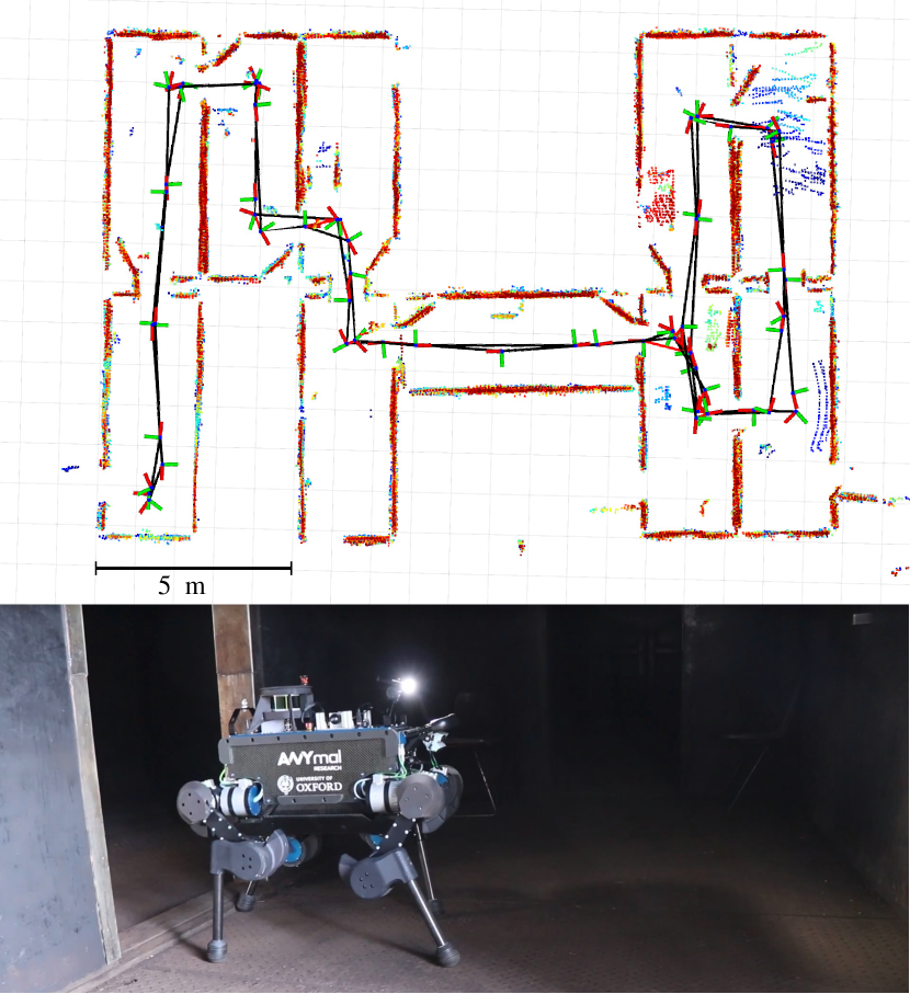
Figure 1: Bird’s-eye view of a map constructed by the ANYmal quadruped exploring an unlit, windowless, industrial facility with our proposed LiDAR-SLAM system. The approach can rapidly detect and verify loop-closures (red lines) so as to construct an accurate map. The approach uses only LiDAR due to the difficult illumination conditions negating the use of visual approaches.

The core odometry of our SLAM system is based on Iterative Closest Point (ICP) registration of 3D point clouds from a LiDAR (Velodyne) sensor. Our approach builds upon our previous work of Autotuning ICP (AICP), originally proposed in [4], which analyzes the content of incoming clouds to robustify registration. Initialization of AICP is provided by the robot’s state estimator[5], which estimates the robot pose by fusing the inertial measurements with the robot’s kinematics and joint information in a recursive approach. Our LiDAR odometry has drift below 1.5$\%$ of distance traveled.

The contributions of our paper are summarized as follows:

1. A LiDAR-SLAM system for legged robots based on ICP registration. The approach uses the robot’s odometry for accurate initialization and a factor graph for global optimization using GTSAM [6].

2. A verification metric which quantifies the reliability of point cloud registration. Inspired by the alignment risk prediction method developed by Nobili et al. [7], we propose a verification system based on efficient k-d tree search [8] to confirm whether a loop closure is well constrained. In contrast to [7], our modified verification method is suitable for online operation.

3. A demonstration of feature-based loop-closure detection which takes advantage of deep learning, specifically designed to be deployable on a mobile CPU during run time. It shows substantially lower computation times when compared to a geometric loop closure method, that scales with the number of surrounding clouds.

4. A real-time demonstration of the algorithm on the ANYmal quadruped robot. We show how the robot can use the map representation to plan safe routes and to autonomously return home on request. We provide detailed quantitative analysis against ground truth maps.

The remainder of this paper is structured as follows: Sec. II presents related works followed by a description of the platform and experimental scenario in Sec. III. Sec. IV details different components of our SLAM system. Sec. V presents evaluation studies before a conclusion and future works are drawn in Sec. VI.

II Related Works

This section provides a literature review of perception in walking robots and LiDAR-SLAM systems in general.

II-A Perception systems on walking robots

Simultaneous Localization and Mapping (SLAM) is a key capability for walking robots and consequently their autonomy. Example systems include, the mono visual SLAM system of [9] which ran on the HRP-2 humanoid robot and is based on an Extended Kalman Filter (EKF) framework. In contrast, [10] leveraged a particle filter to estimate the posterior of their SLAM method, again on HRP-2. Oriolo et al. [11] demonstrated visual odometry on the Nano bipedal robot by tightly coupling visual information with the robot’s kinematics and inertial sensing within an EKF. However, these approaches were reported to acquire only a sparse map of the environment on the fly, substantially limiting the robot’s perception.

Ahn et al. [12] presented a vision-aided motion estimation framework for the Roboray humanoid robot by integrating visual-kinematic odometry with inertial measurements. Furthermore, they employed the pose estimation to reconstruct a 3D voxel map of the environment utilizing depth data from a Time-of-Flight camera. However, they did not integrate the depth data for localization purposes.

Works such as [13] and [14] leveraged the frame-to-model visual tracking of KinectFusion [15] or ElasticFusion [16], which use a coarse-to-fine ICP algorithm. Nevertheless, vision-based SLAM techniques struggle in varying illumination conditions. While this has been explored in works such as [17] and [3], it remains an open area of research. In addition, the relatively short range of visual observations limit their performance for large-scale operations.

A probabilistic localization approach exploiting LiDAR information was implemented by Hornung et al. [18] on the Nao humanoid robot. Utilizing a Bayes filtering method, they integrated the measurements from a 2D range finder with a motion model to recursively estimate the pose of the robot’s torso. They did not address the SLAM problem directly since they assumed the availability of a volumetric map for step planning.

Compared to bipedal robots, quadrupedal robots have better versatility and resilience when navigating challenging terrain. Thus, they are more suited to long-term tasks such as inspection of industrial sites. In the extreme case, a robot might need to jump over a terrain hurdle. Park et al., in [19], used a Hokuyo laser range finder on the MIT Cheetah 2 to detect the ground plane as well as the front face of a hurdle. Although, the robot could jump over hurdles as high as 40 cm, the LiDAR measurements were not exploited to contribute to the robot’s localization.

Nobili et al. [20] presented a state estimator for the Hydraulic Quadruped robot which took advantage of a variety of sensors, including inertial, kinematic and LiDAR measurements. Based on a modular inertial-driven EKF, the robot’s base link velocity and position were propagated using measurements from modules including leg odometry, visual odometry and LiDAR odometry. Nevertheless, the system is likely to suffer from drift over the course of a large trajectory, as the navigation system did not include a mechanism to detect loop-closures.

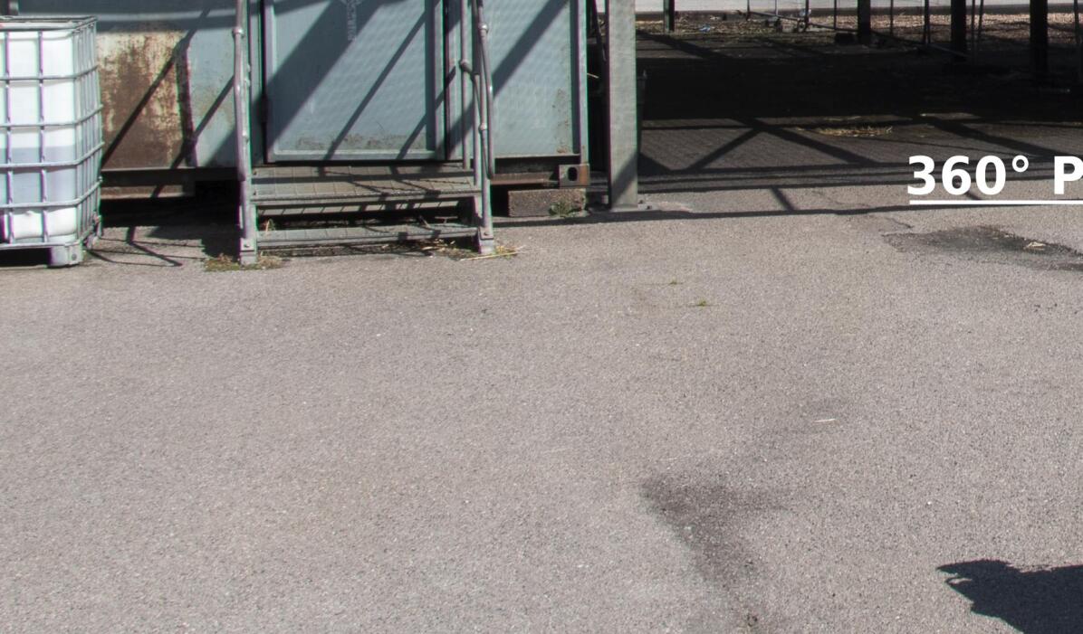
Figure 2: Our experiments were carried out with the quadrupedal robot, ANYmal, in the Oil Rig training site at the Fire Service College, Moreton-in-Marsh, UK. To determine ground truth robot poses, we used a Leica TS16 laser tracker to track a $360^{\circ}$ prism on the robot.

II-B LiDAR-SLAM Systems

The well-known method for point cloud registration is ICP which is used in a variety of application [21]. Given an initialization for the sensor pose, ICP iteratively estimates the relative transformation between two point clouds. A standard formulation of ICP minimizes the distance between corresponding points or planes after data filtering and outlier rejection. However, ICP suffers from providing a good solution in ill-conditioned situations such as when the robot crosses a door way.

An effective LiDAR-based approach is LiDAR Odometry and Mapping (LOAM) [22]. LOAM extracts edge and surface point features in a LiDAR cloud by evaluating the roughness of the local surface. The features are reprojected to the start of the next scan based on a motion model, with point correspondences found within this next scan. Finally, the 3D motion is estimated recursively by minimizing the overall distances between point correspondences. LOAM achieves high accuracy and low cost of computation.

Shan et al. in [23] extended LOAM with Lightweight and Ground-Optimized LiDAR Odometry and Mapping (LeGO-LOAM) which added latitudinal and longitudinal parameters separately in a two-phase optimization. In addition, LeGO-LOAM detected loop-closures using an ICP algorithm to create a globally consistent pose graph using iSAM2 [24].

Dubé et al. in [25] developed an online cooperative LiDAR-SLAM system. Using two and three robots, each equipped with 3D LiDAR, an incremental sparse pose-graph is populated by successive place recognition constraints. The place recognition constraints are identified utilizing the SegMatch algorithm [26], which represents LiDAR clouds as a set of compact yet discriminative features. The descriptors were used in a matching process to determine loop closures.

Our approach is most closely related to the localization system in [20]. However, in order to have a globally consistent map and to maintain drift-free global localization, we build a LiDAR-SLAM on top of the AICP framework which enables detection of loop-closures and adds these constraints to a factor-graph. Furthermore, we develop a fast verification of point-cloud registrations to effectively avoid incorrect factors to be added to the pose graph. We explain each component of our work in Sec. IV.

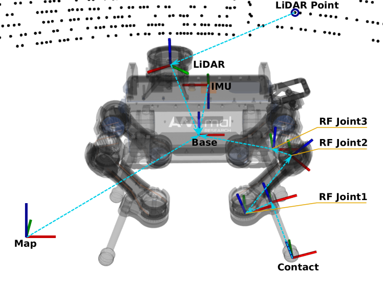
Figure 3: Axis conventions of various frames used in the LiDAR-SLAM system and their relationship with respect to the base frame. As an example, we show only the Right Front (RF) leg.

III Platform and Experimental Scenario

We employ a state-of-the-art quadruped, ANYmal (version B) [27], as our experimental platform. Fig. 2 shows a view of the ANYmal robot. The robot weighs about $33$ $\mathrm{k}\mathrm{g}$ without any external perception modules and can carry a maximum payload of $10$ $\mathrm{k}\mathrm{g}$ at the maximum speed of $1.0$ $\mathrm{m}\mathrm{/}\mathrm{s}$. As shown in Fig. 3, each leg contains 3 actuated joints which altogether gives 18 degrees of freedom, 12 actuated joints and the 6 DoF robot base, which the robot uses to dynamically navigate challenging terrain.

Tab. I summarizes the specifications of the robot’s sensors. The high frequency sensors (IMU, joint encoders and torque sensors) are tightly coupled through a Kalman filtering approach [28] on the robot’s Locomotion Personal Computer (LPC). Navigation measurements from the Velodyne VLP-16 LiDAR sensor and the robot’s cameras are processed on a separate on-board computer to achieve online localization and mapping, as well as other tasks such as terrain mapping and obstacle avoidance. The pose estimate of our LiDAR-SLAM system is fed back to the LPC for path planning.

Sensor	Model	Frequency	Specifications
		Bias Repeatability: $<0.5^{\circ}/s$; $~{}5$ $mg$
IMU	Xsens	$400$
	MTi-100		Bias Stability: $10^{\circ}/h$; $40$ $\mu g$
	Velodyne	$10$	Resolution in Azimuth: $<0.4^{\circ}$
LiDAR	VLP-16		Resolution in Zenith: $2.0^{\circ}$
Unit			Range $<100$ $m$
			Accuracy: $\pm$ $3$ $cm$
Encoder	ANYdrive	$400$	Resolution $<0.025^{\circ}$
Torque	ANYdrive	$400$	Resolution $<0.1$ $Nm$

TABLE I: Specifications of the sensors installed on the ANYmal.

IV Approach

Our goal is to provide the quadrupedal robot with a drift-free localization estimate over the course of a very long mission, as well as to enable the robot to accurately map its surroundings. The on-the-fly map can further be employed for the purpose of optimal path planning as edges on the factor graph also indicate safe and traversable terrain. Fig. 4 elucidates the different components of our system.

We correct the pose estimate of the kinematic-inertial odometry by the LiDAR data association in a loosely-coupled fashion.

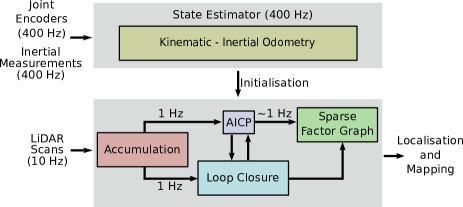
Figure 4: Block diagram of the LiDAR-SLAM system.

IV-A Kinematic-Inertial Odometry

The proprioceptive sensors are tightly coupled using a recursive error-state estimator, Two-State Implicit Filter (TSIF) [28], which estimates the incremental motion of the robot. By assuming that each leg is in stationary contact with the terrain, the position of the contact feet in the inertial frame $\{\mathcal{I}\}$, obtained from forward kinematics, is treated as a temporal measurement to estimate the robot’s pose in the fixed odometry frame, $\{\mathcal{O}\}$:

$$\textbf{T}_{\mathcal{B}}^{\mathcal{O}}=\begin{bmatrix}\textbf{R}_{\mathcal{B}}^{\mathcal{O}}&\textbf{p}_{\mathcal{B}}^{\mathcal{O}}\\ \text{0}&1\end{bmatrix},$$ (1)

where $\textbf{T}_{\mathcal{B}}^{\mathcal{O}}\in SE(3)$ is the transformation from the base frame $\{\mathcal{B}\}$ to the odometry frame $\{\mathcal{O}\}$.

This estimate of the base frame drifts over time as it does not use any exteroceptive sensors and the position of the quadruped and its rotation around $z$-axis are not observable. In the following, we define our LiDAR-SLAM system for estimation of the robot’s pose with respect to the map frame $\{\mathcal{M}\}$ which is our goal. It is worth noting that the TSIF framework estimates the covariance of the state [28] which we employ during our geometric loop-closure detection.

IV-B LiDAR-SLAM System

Our LiDAR-SLAM system is a pose graph SLAM system built upon our ICP registration approach called Autotuned-ICP (AICP) [4]. AICP automatically adjusts the outlier filter of ICP by computing an overlap parameter, $\Omega\in[0,1]$ since the assumption of a constant overlap, which is conventional in the standard outlier filters, violates the registration in real scenarios.

Given the initial estimated pose from the kinematic-inertial odometry, we obtain a reference cloud to which we align each consecutive reading point cloud.

In this manner the successive reading clouds are precisely aligned with the reference clouds with greatly reduced drift. The robot’s pose, corresponding to each reading cloud is obtained as follows:

$$\textbf{T}_{\mathcal{B}}^{\mathcal{M}}=\Delta_{aicp}\textbf{T}_{\mathcal{B}}^{\mathcal{O}},$$ (2)

where $\textbf{T}_{\mathcal{B}}^{\mathcal{M}}$ is the robot’s pose in the map frame $\{\mathcal{M}\}$ and $\Delta_{aicp}$ is the alignment transformation calculated by AICP.

Calculating the corrected poses, corresponding to the point clouds, we compute the relative transformation between the successive reference clouds to create the odometry factors of the factor graph which we introduce in Eq. (3).

The odometry factor, $\phi_{i}(\mathcal{X}_{i-1},\mathcal{X}_{i})$, is defined as:

$$\phi_{i}(\mathcal{X}_{i-1},\mathcal{X}_{i})=(\textbf{T}_{\mathcal{B}_{i-1}}^{\mathcal{M}^{-1}}\textbf{T}_{\mathcal{B}_{i}}^{\mathcal{M}})^{-1}\widetilde{\textbf{T}}_{\mathcal{B}_{i-1}}^{\mathcal{M}^{-1}}\widetilde{\textbf{T}}_{\mathcal{B}_{i}}^{\mathcal{M}},$$ (3)

where $\widetilde{\textbf{T}}_{\mathcal{B}_{i-1}}^{\mathcal{M}}$ and $\widetilde{\textbf{T}}_{\mathcal{B}_{i}}^{\mathcal{M}}$ are the AICP estimated poses of the robot for the node $\mathcal{X}_{i-1}$ and $\mathcal{X}_{i}$, respectively, and $\textbf{T}_{\mathcal{B}_{i-1}}^{\mathcal{M}}$ and $\textbf{T}_{\mathcal{B}_{i}}^{\mathcal{M}}$ are the noise-free transformations.

A prior factor, $\phi_{0}(\mathcal{X}_{0})$, which is taken from the pose estimate of the kinematic-inertial odometry, is initially added to the factor graph to set an origin and a heading for the robot within the map frame $\{\mathcal{M}\}$.

To correct for odometric drift, loop-closure factors are added to the factor graph once the robot revisits an area of the environment. We implemented two approaches for proposing loop-closures: a) geometric proposal based on the distance between the current pose and poses already in the factor graph which is useful for smaller environments, and b) a learning approach for global loop-closure proposal, detailed in Sec IV-C1, which scales to large environments. Each proposal provides an initial guess, which is refined with ICP.

Each individual loop closure becomes a factor and is added to the factor graph. The loop-closure factor, in this work, is a factor whose end is the current pose of the robot and whose start is one of the reference clouds, stored in the history of the robot’s excursion. The nominated reference cloud must meet two criteria of nearest neighbourhood and sufficient overlap with the current reference cloud. An accepted loop-closure factor, $\phi_{j}(\mathcal{X}_{M},\mathcal{X}_{N})$, is defined as:

$$\phi_{j}({\mathcal{X}_{M},\mathcal{X}_{N}})=(\textbf{T}_{\mathcal{B}_{M}}^{\mathcal{M}^{-1}}\textbf{T}_{\mathcal{B}_{N}}^{\mathcal{M}})^{-1}(\Delta_{j,aicp}\widetilde{\textbf{T}}_{\mathcal{B}_{M}}^{\mathcal{M}})^{-1}\widetilde{\textbf{T}}_{\mathcal{B}_{N}}^{\mathcal{M}},$$ (4)

where $\widetilde{\textbf{T}}_{\mathcal{B}_{M}}^{\mathcal{M}}$ and $\widetilde{\textbf{T}}_{\mathcal{B}_{N}}^{\mathcal{M}}$ are the robot’s poses in the map frame $\{\mathcal{M}\}$ corrected by AICP with respect to the reference cloud $(M-1)$ and the reference cloud $(N-1)$, respectively. The $\Delta_{j,aicp}$ is the AICP correction between the current reference cloud $M$ and the nominated reference cloud $N$.

Once all the factors, including odometry and loop-closure factors, have been added to the factor graph, we optimize the graph so that we find the Maximum A Posteriori (MAP) estimate for the robot poses corresponding to the reference clouds. To carry out this inference over the variables $\mathcal{X}_{i}$, where $i$ is the number of the robot’s pose in the factor graph, the product of all the factors, must be maximized:

$$\mathcal{X}^{MAP}=\ \operatorname*{argmax}_{\mathcal{X}}\ \prod_{i}\phi_{i}(\mathcal{X}_{i-1},\mathcal{X}_{i})\prod_{j}\phi_{j}(\mathcal{X}_{M},\mathcal{X}_{N}).$$ (5)

Assuming that factors follow a Gaussian distribution and all measurements are only corrupted with white noise, i.e. noise with normal distribution and zero mean, the optimization problem in Eq. (5) is equivalent to minimizing a sum of nonlinear least squares:

$$\begin{split}\mathcal{X}^{MAP}=\ \operatorname*{argmin}_{\mathcal{X}}\sum_{i}||y_{i}(\mathcal{X}_{i},\mathcal{X}_{i-1})-m_{i}||^{2}_{\bm{\Sigma}_{i}}\\ +\sum_{j}||y_{j}(\mathcal{X}_{M},\mathcal{X}_{N})-m_{j}||^{2}_{\bm{\Sigma}_{j}},\end{split}$$ (6)

where $m$, $y$ and $\bm{\Sigma}$ denote the measurements, their mathematical model and the covariance matrices, respectively.

As noted, the MAP estimate is only reliable when the residuals in Eq. (6) follow the normal distribution. However, ICP is susceptible to failure in the absence of geometric features, e.g. in corridors or door entries, which can have a detrimental effect when optimizing the pose graph. In Sec. IV-D, we propose a fast verification technique for point cloud registration to detect possible failure of the AICP registration.

1 input: source, target clouds $\mathcal{C}_{S}$, $\mathcal{C}_{T}$; estimated poses $\mathcal{X}_{S}$, $\mathcal{X}_{T}$

2 output: alignment risk $\rho=f(\Omega,\alpha)$

3 begin

4       Segment $\mathcal{C}_{S}$ and $\mathcal{C}_{T}$ into a set of planes: $P_{Si}$ and $P_{Tj}$ $i\in N_{S}$, $j\in N_{T}$,

5       Compute centroid of each plane (Keypoint): $\bm{K}_{Si}$, $\bm{K}_{Tj}$,

6       Transform query keypoints $\bm{K}_{Tj}$ into the space of $\mathcal{C}_{S}$,

7       Search the nearest neighbour of each query plane $P_{Tj}$ using a k-d tree,

8       for plane $P_{T}$ do

9            Find match $P_{S}$ amongst candidates in the k-d tree,

10             Compute the matching score $\Omega_{p}$,

11             if $\Omega_{p}$ is max then

12                  Determine the normal of plane $P_{T}$,

13                   Push back the normal into the matrix $\bm{N}$,

14             end if

15            

16       end for

17      Compute alignability $\alpha=\lambda_{max}\mathbin{/}\lambda_{min}$;

18       Learn $\rho=f(\Omega,\alpha)$;

19       Return $\rho$;

20 end

21

Algorithm 1 Improved Risk Alignment Prediction.

IV-C Loop Proposal Methods

This section introduces our learned loop-closure proposal and geometric loop-closure detection.

IV-C1 Deeply-learned Loop Closure Proposal

We use the method of Tinchev et al. [30], which is based on matching individual segments in pairs of point clouds using a deeply-learned feature descriptor. Its specific design uses a shallow network such that it does not require a GPU during run-time inference on the robot. We present a summary of the method called Efficient Segment Matching (ESM), but refer the reader to [30].

First, a neural network is trained offline using individual LiDAR observations (segments). By leveraging odometry in the process, we can match segment instances without manual intervention. The input to the network is a batch of triplets - anchor, positive and negative segments. The anchor and positive samples are the same object from two successive Velodyne scans, while the negative segment is a segment chosen $\approx 20\,\text{m}$ apart. The method then performs a series of $X\text{-conv}$ operators directly on raw point cloud data, based on PointCNN [31], followed by three fully connected layers, where the last layer is used as the descriptor for the segments.

During our trials, when the SLAM system receives a new reference cloud, it is preprocessed and then segmented into a collection of point cloud clusters. These clusters are not semantically meaningful, but they broadly correspond to physical objects such as a vehicle, a tree or building facade. For each segment in the reference cloud, a descriptor vector is computed with an efficient TensorFlow C++ implementation by performing a forward pass using the weights from the already trained model. This allows a batch of segments to be preprocessed simultaneously with zero-meaning and normalized variance and then forward passed through the trained model. We use a three dimensional tensor as input to the network - the length is the number of segments in the current point cloud, the width represents a fixed-length down-sampled vector of all the points in an individual segment, and the height contains the $x$, $y$ and $z$ values. Due to the efficiency of the method, we need not split the tensor into mini-batches, allowing us to process the full reference cloud in a single forward pass.

Once the descriptors for the reference cloud are computed, they are compared to the map of previous reference clouds. ESM uses an $l_{2}$ distance in feature space to detect matching segments and a robust estimator to retrieve a 6DoF pose. This produces a transformation of the current reference cloud with respect to the previous reference clouds. The transformation is then used in AICP to add a loop-closure as a constraint to the graph-based optimization. Finally, ESM’s map representation is updated, when the optimization concludes.

IV-C2 Geometric Loop-Closure Detection

To geometrically detect loop-closures, we use the covariance of the legged state estimator (TSIF) to define a dynamic search window around the current pose of the robot. Then the previous robot’s poses, which reside within the search window, are examined based on two criteria: nearest neighbourhood and verification of cloud registration (described in Sec. IV-D). Finally, the geometric loop closure is computed between the current cloud and the cloud corresponding to the nominated pose using AICP.

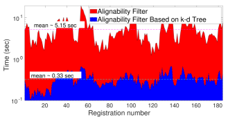
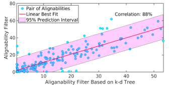
Figure 5: Comparison of our proposed verification method with the original in terms of computation time (left) and performance (right).

IV-D Fast Verification of Point Cloud Registration

This section details a verification approach for ICP point cloud registration to determine if two point clouds can be safely registered. We improve upon our previously proposed alignability metric in [7] with a much faster method.

Method from [7]: First, the point clouds are segmented into a set of planar surfaces. Second, a matrix $\bm{N}\in\mathbb{R}^{M\times 3}$ is computed, where each row corresponds to the normal of the planes ordered by overlap. $M$ is the number of matching planes in the overlap region between the two clouds. Finally, the alignability metric, $\alpha$ is defined as the ratio between the smallest and largest eigenvalues of $\bm{N}$.

The matching score, $\Omega_{p}$, is computed as the overlap between two planes, $P_{Tj}$ and $P_{Si}$ where $i\in N_{S}$ and $j\in N_{T}$. $N_{S}$ and $N_{T}$ are the number of planes in the input clouds. In addition, in order to find the highest possible overlap, the algorithm iterates over all possible planes from two point clouds. This results in overall complexity $O(N_{S}N_{T}(N_{P_{S}}N_{P_{T}}))$, where $N_{P_{S}}$ and $N_{P_{T}}$ are the average number of points in planes of the two clouds.

Proposed Improvement: To reduce the pointwise computation, we first compute the centroids of each plane $\bm{K}_{Si}$ and $\bm{K}_{Tj}$ and align them from point cloud $\mathcal{C}_{T}$ to $\mathcal{C}_{S}$ given the computed transformation. We then store the centroids in a k-d tree and for each query plane $P_{T}\in\mathcal{C}_{T}$ we find the $K$ nearest neighbours. We compute the overlap for the $K$ nearest neighbours, and use the one with the highest overlap. This results in $O(N_{T}K(N_{P_{S}}N_{P_{T}}))$, where $K<<N_{s}$. In practice, we found that $K=1$ is sufficient for our experiments. Furthermore, we only store the centroids in a k-d tree, reducing the space complexity.

We discuss the performance of this algorithm, as well as its computational complexity in the experiment section of this paper. Pseudo code of the algorithm is available in Algorithm 1.

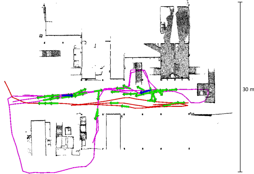
Figure 6: Demonstration of the learning-based loop closure in the outdoor experiment. 249 point clouds from two different runs were first registered against a ground truth Leica map (black). The red and magenta traces correspond to the traversed path of each run. Just two Velodyne point clouds are used to form a map for ESM (blue arrows). Successful loop closures from the 50 clouds (green arrows) demonstrate robustness to viewpoint variation/offset.

V Experimental Evaluation

The proposed LiDAR-SLAM system is evaluated using the datasets collected by our ANYmal quadruped robot. We first analyze the verification method. Second, we investigate the learned loop-closure detection in terms of speed and reliability (Sec. V-B). We then demonstrate the performance or our SLAM system on two large-scale experiments, one indoor and one outdoor (Sec. V-C) including an online demonstration where the map is used for route following (Sec. V-D). A demonstration video can be found at
https://ori.ox.ac.uk/lidar-slam.

V-A Verification Performance

We focus on the alignability metric $\alpha$ of the alignment risk prediction since it is our primary contribution. We computed $\alpha$ between consecutive point clouds of our outdoor experiment, which we discuss later in Sec. V-C. As seen in Fig. 5 (Left), the alignability filter based on a k-d tree is substantially faster than the original filter. As noted in Sec. IV-D, our approach is less dependent on the point cloud size, due to only using the plane centroids. Whereas, the original alignability filter fully depends on all the points of the segments, resulting in higher computation time. Having tested our alignability filter for the datasets taken from Velodyne VLP-16, the average computation time is less than 0.5 seconds (almost 15x improvement) which is suitable for real-time operation.

Fig. 5 (Right) shows that our approach highly correlates with the result from the original approach. Finally, we refer the reader to the original work that provided a thorough comparison of alignment risk against Inverse Condition Number (ICN) [32] and Degeneracy parameter [33] in ill-conditioned scenarios. The former mathematically assessed the condition of the optimization, whereas the latter determines the degenerate dimension of the optimization.

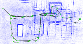
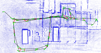
(a) AICP Odometry without loop-closure (b) SLAM without loop-closure verification

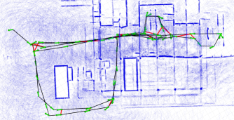
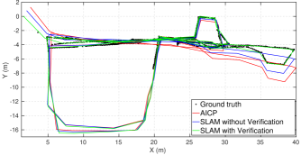
(c) SLAM with loop-closure verification (d) Comparison against ground truth

Figure 7: Illustration of different algorithm variants: (a) AICP odometry, (b) the SLAM system without verification enabled (c) the SLAM system with it enabled, and finally (d) a comparison of their estimated trajectories with poses from Leica tracker (ground truth).

V-B Evaluation of Learned Loop Closure Detector

In the next experiment we explore the performance of the different loop closure methods using a dataset collected outdoors at the Fire Service College, Moreton-in-Marsh, UK.

V-B1 Robustness to viewpoint variation

Fig. 6 shows a preview of our SLAM system with the learned loop closure method. We selected just two point clouds to create the map, with their positions indicated by the blue arrows in Fig. 6.

The robot executed two runs in the environment, which comprised 249 point clouds. We deliberately chose to traverse an offset path (red) the second time so as to determine how robust our algorithm is to translation and viewpoint variation. In total 50 loop closures were detected (green arrows) around the two map point clouds. Interestingly, the approach not only detected loop closures from both trajectories, with translational offsets up to 6.5 m, but also with orientation variation up to $180^{\circ}$- something not achievable by standard visual localization - a primary motivation for using LiDAR. Across the 50 loop closures an average of $5.24$ segments were recognised per point cloud. The computed transformation had an Root Mean Square Error (RMSE) of $0.08\pm 0.02\,\text{m}$ from the ground truth alignment. This was achieved in approximately $486\,\text{ms}$ per query point cloud.

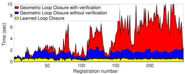
Figure 8: Computation times of the considered loop closure methods. The computation time increases when the robot revisits old parts of the map, affecting the speed of geometric loop-closure detection, specifically when verification is enabled.

V-B2 Computation Time

Fig. 8 shows a graph of the computation time. The computation time for the geometric loop closure method depends on the number of traversals around the same area. The geometric loop closures iterated over the nearest $N$ clouds, based on a radius; the covariance and distance travelled caused it to slow down. Similarly, the verification method needs to iterate over large proportion of the point clouds in the same area, affecting the real time operation.

Instead, the learning loop closure proposal scales better with map size. It compares low dimensional feature descriptor vectors, which is much faster than the thousands of data points in Euclidean space.

V-C Indoor and Outdoor Experiments

To evaluate the complete SLAM system, the robot walked indoor and outdoor along trajectories with the length of about 100 m and 250 m, respectively. Each experiment lasted about 45 minutes. Fig. 1 (Bottom) and Fig. 2 illustrate the test locations: industrial buildings. For quality evaluation, we compared the SLAM system, AICP, and the legged odometry (TSIF) using ground truth. As shown in Fig. 2, we used a Leica TS16 to automatically track a $360^{\circ}$ prism rigidly mounted on top of the robot. This way, we managed to record the robot’s position with millimeter accuracy at about 7 Hz (when in line of sight).

For evaluation metrics, we use Relative Pose Error (RPE) and Absolute Trajectory Error (ATE) [34]. RPE determines the regional accuracy of the trajectory over time. In other words, it is a metric which measures the drift of the estimated trajectory. ATE is the RMSE of the Euclidean distance between the estimated trajectory and the ground truth. ATE validates the global consistency of the estimated trajectory.

As seen in Fig. 7, our SLAM system is almost complete consistent with the ground truth. The verification algorithm approved 27 loop-closure factors (indicated in red) which were added to the factor graph. Without this verification 38 loop-closures were created, some in error, resulting in an inferior map.

Tab. II reports SLAM results with and without verification compared to the AICP LiDAR odometry and the TSIF legged state estimator. As the Leica TS16 does not provide rotational estimates, we took the best performing method - SLAM with verification - and compared the rest of the trajectories to it with the ATE metric. Based on this experiment, the drift of SLAM with verification is less than 0.07$\%$, satisfying many location-based tasks of the robot.

For the indoor experiment, the robot walked along narrow passages with poor illumination and indistinct structure. Due to the lack of ground truth, only estimated trajectories are only displayed in Fig. 9, with the map generated by SLAM with verification. As indicated, in points A, B and C, AICP approach cannot provide sufficient accuracy for the robot to safely pass through doorways about 1 m wide.

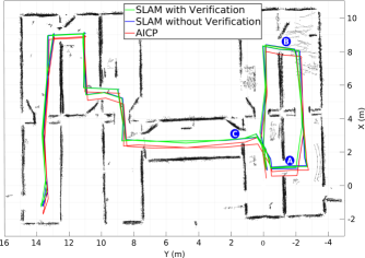
Figure 9: Estimated trajectories for the indoor experiment, overlayed on the map created by the SLAM system using the verification approach.

	Translational	Heading	Relative Pose
Method	Error (RMSE) (m)	Error (RMSE) (deg)	Error (m)
SLAM with Verification	0.06	N/A	0.090
SLAM without Verification	0.23	1.6840	0.640
AICP (LiDAR odometry)	0.62	3.1950	1.310
TSIF (legged odometry)	5.40	36.799	13.64

TABLE II: Comparison of the localization accuracy for the different approaches.

V-D Experiments on the ANYmal

In a final experiment, we tested the SLAM system online on the ANYmal. After building a map with several loops (while teleoperated), we queried a path back to the operator station. Using the Dijkstra’s algorithm [35], the shortest path was created using the factor graph. As each edge has previously been traverse, following the return trajectory returned the robot to the starting location. The supplementary video demonstrates the experiment.

VI Conclusion and Future Work

This paper presented an accurate and robust LiDAR-SLAM system on a resource constrained legged robot using a factor graph-based optimization. We introduced an improved registration verification algorithm capable of running in real time. In addition, we leveraged a state-of-the-art learned loop closure detector which is sufficiently efficient to run online and had significant viewpoint robustness. We examined our system in indoor and outdoor industrial environments with a final demonstration showing online operation of the system on our robot.

In the future, we will speed up our ICP registration to increase the update frequency in our SLAM system. We will also examine our system in more varied scenarios enabling real-time tasks on the quadruped ANYmal. In addition, we would like to integrate visual measurements taken from the robot’s RGBD camera to improve initialization of point cloud registration as well as independent registration verification.

References

- [1] R. Mur-Artal, J. M. M. Montiel, and J. D. Tardos, “ORB-SLAM: a versatile and accurate monocular SLAM system,” TRO, 2015.
- [2] J. Engel, T. Schöps, and D. Cremers, “LSD-SLAM: Large-scale direct monocular SLAM,” in ECCV, 2014.
- [3] H. Porav, W. Maddern, and P. Newman, “Adversarial training for adverse conditions: Robust metric localisation using appearance transfer,” in ICRA, 2018.
- [4] S. Nobili, R. Scona, M. Caravagna, and M. Fallon, “Overlap-based ICP tuning for robust localization of a humanoid robot,” in ICRA, 2017.
- [5] M. Bloesch, M. Hutter, M. A. Hoepflinger, S. Leutenegger, C. Gehring, C. D. Remy, and R. Siegwart, “State estimation for legged robots-consistent fusion of leg kinematics and IMU,” in RSS, 2013.
- [6] F. Dellaert, “Factor graphs and gtsam: A hands-on introduction,” Georgia Institute of Technology, Tech. Rep., 2012.
- [7] S. Nobili, G. Tinchev, and M. Fallon, “Predicting alignment risk to prevent localization failure,” in ICRA, 2018.
- [8] J. L. Bentley, “Multidimensional binary search trees used for associative searching,” CACM, 1975.
- [9] O. Stasse, A. Davison, R. Sellaouti, and K. Yokoi, “Real-time 3D slam for humanoid robot considering pattern generator information,” in IROS, 2006.
- [10] N. Kwak, O. Stasse, T. Foissotte, and K. Yokoi, “3D grid and particle based slam for a humanoid robot,” in Humanoids, 2009.
- [11] G. Oriolo, A. Paolillo, L. Rosa, and M. Vendittelli, “Vision-based odometric localization for humanoids using a kinematic EKF,” in Humanoids, 2012.
- [12] S. Ahn, S. Yoon, S. Hyung, N. Kwak, and K. S. Roh, “On-board odometry estimation for 3D vision-based SLAM of humanoid robot,” in IROS, 2012.
- [13] R. Wagner, U. Frese, and B. Bäuml, “Graph SLAM with signed distance function maps on a humanoid robot,” in IROS, 2014.
- [14] R. Scona, S. Nobili, Y. R. Petillot, and M. Fallon, “Direct visual SLAM fusing proprioception for a humanoid robot,” in IROS, 2017.
- [15] R. Newcombe, S. Izadi, O. Hilliges, D. Molyneaux, D. Kim, A. Davison, P. Kohli, J. Shotton, S. Hodges, and A. Fitzgibbon, “KinectFusion: Real-time dense surface mapping and tracking.” in ISMAR, 2011.
- [16] T. Whelan, S. Leutenegger, R. Salas-Moreno, B. Glocker, and A. Davison, “ElasticFusion: Dense SLAM without a pose graph.” RSS, 2015.
- [17] M. Milford and G. Wyeth, “SeqSLAM: Visual route-based navigation for sunny summer days and stormy winter nights,” in ICRA, 2012.
- [18] A. Hornung, K. M. Wurm, and M. Bennewitz, “Humanoid robot localization in complex indoor environments,” in IROS, 2010.
- [19] H.-W. Park, P. Wensing, and S. Kim, “Online planning for autonomous running jumps over obstacles in high-speed quadrupeds,” in RSS, 2015.
- [20] S. Nobili, M. Camurri, V. Barasuol, M. Focchi, D. Caldwell, C. Semini, and M. Fallon, “Heterogeneous sensor fusion for accurate state estimation of dynamic legged robots,” in RSS, 2017.
- [21] F. Pomerleau, “Applied registration for robotics: Methodology and tools for ICP-like algorithms,” Ph.D. dissertation, ETH Zurich, 2013.
- [22] J. Zhang and S. Singh, “LOAM: Lidar Odometry and Mapping in real-time.” in RSS, 2014.
- [23] T. Shan and B. Englot, “LeGO-LOAM: Lightweight and ground-optimized LiDAR odometry and mapping on variable terrain,” in IROS, 2018.
- [24] M. Kaess, H. Johannsson, R. Roberts, V. Ila, J. Leonard, and F. Dellaert, “iSAM2: Incremental smoothing and mapping using the bayes tree,” IJRR, 2012.
- [25] R. Dubé, A. Gawel, H. Sommer, J. Nieto, R. Siegwart, and C. Cadena, “An online multi-robot SLAM system for 3D LiDARS,” in IROS, 2017.
- [26] R. Dubé, D. Dugas, E. Stumm, J. Nieto, R. Siegwart, and C. Cadena, “Segmatch: Segment based place recognition in 3D point clouds,” in ICRA, 2017.
- [27] M. Hutter, C. Gehring, D. Jud, A. Lauber, C. D. Bellicoso, V. Tsounis, J. Hwangbo, K. Bodie, P. Fankhauser, and M. Bloesch, “Anymal - a highly mobile and dynamic quadrupedal robot,” in IROS, 2016.
- [28] M. Bloesch, M. Burri, H. Sommer, R. Siegwart, and M. Hutter, “The two-state implicit filter recursive estimation for mobile robots,” RAL, 2017.
- [29] F. Pomerleau, F. Colas, R. Siegwart, and S. Magnenat, “Comparing icp variants on real-world data sets,” Autonomous Robots, 2013.
- [30] G. Tinchev, A. Penate-Sanchez, and M. Fallon, “Learning to see the wood for the trees: Deep laser localization in urban and natural environments on a CPU,” RAL, 2019.
- [31] Y. Li, R. Bu, M. Sun, W. Wu, X. Di, and B. Chen, “PointCNN: Convolution on X-transformed points,” in NIPS, 2018.
- [32] E. Cheney and D. Kincaid, Numerical mathematics and computing. Cengage Learning, 2012.
- [33] J. Zhang, M. Kaess, and S. Singh, “On degeneracy of optimization-based state estimation problems,” in ICRA, 2016.
- [34] J. Sturm, N. Engelhard, F. Endres, W. Burgard, and D. Cremers, “A benchmark for the evaluation of RGB-D SLAM systems,” in IROS, 2012.
- [35] E. Dijkstra, “A note on two problems in connexion with graphs,” Numerische mathematik, 1959.