Large-time behavior of solutions of parabolic equations on the real line with convergent initial data II: equal limits at infinity

Abstract

We continue our study of bounded solutions of the semilinear parabolic equation $u_{t}=u_{xx}+f(u)$ on the real line, where $f$ is a locally Lipschitz function on $\mathbb{R}.$ Assuming that the initial value $u_{0}=u(\cdot,0)$ of the solution has finite limits $\theta^{\pm}$ as $x\to\pm\infty$, our goal is to describe the asymptotic behavior of $u(x,t)$ as $t\to\infty$. In a prior work, we showed that if the two limits are distinct, then the solution is quasiconvergent, that is, all its locally uniform limit profiles as $t\to\infty$ are steady states. It is known that this result is not valid in general if the limits are equal: $\theta^{\pm}=\theta_{0}$. In the present paper, we have a closer look at the equal-limits case. Under minor non-degeneracy assumptions on the nonlinearity, we show that the solution is quasiconvergent if either $f(\theta_{0})\neq 0$, or $f(\theta_{0})=0$ and $\theta_{0}$ is a stable equilibrium of the equation $\dot{\xi}=f(\xi)$. If $f(\theta_{0})=0$ and $\theta_{0}$ is an unstable equilibrium of the equation $\dot{\xi}=f(\xi)$, we also prove some quasiconvergence theorem making (necessarily) additional assumptions on $u_{0}$. A major ingredient of our proofs of the quasiconvergence theorems—and a result of independent interest—is the classification of entire solutions of a certain type as steady states and heteroclinic connections between two disjoint sets of steady states.

Key words: Parabolic equations on $\mathbb{R}$, quasiconvergence, entire solutions, chains, connecting orbits, zero number, spatial trajectories, Morse decompositions

1 Introduction and main results

1.1 Background

Consider the Cauchy problem

$$u_{t}=u_{xx}+f(u), \qquad x\in\mathbb{R},\ t>0,$$ (1.1)

$$u(x,0)=u_{0}(x), \qquad x\in\mathbb{R},$$ (1.2)

where $f$ is a locally Lipschitz function on $\mathbb{R}$ and $u_{0}\in C_{b}(\mathbb{R}):=C(\mathbb{R})\cap L^{\infty}(\mathbb{R}).$ We denote by $u(\cdot,t,u_{0}),$ or simply $u(\cdot,t)$ if there is no danger of confusion, the unique classical solution of (1.1), (1.2) and by $T(u_{0})\in(0,+\infty]$ its maximal existence time. If $u$ is bounded on $\mathbb{R}\times[0,T(u_{0}))$, then necessarily $T(u_{0})=+\infty,$ that is, the solution is global. In this paper, we are concerned with the behavior of bounded solutions as $t\to\infty$. A basic question we specifically want to address is whether, or to what extent, the large-time behavior of bounded solutions is governed by steady states of (1.1).

If the initial data $u_{0}$ admits limits as $x\to\pm\infty,$ then for all time $t>0,$ the solution $u(\cdot,t)$ of (1.1), (1.2) admits limits as $x\to\pm\infty.$ In other words, the function space

$$\mathcal{V}:=\left\{v\in C_{b}(\mathbb{R}):\textrm{ the limits }v(-\infty),\,v(+\infty)\in\mathbb{R}\textrm{ exist}\right\}$$ (1.3)

is invariant for (1.1). Continuing our study initiated in [29], we examine the large time behavior of bounded solutions in ${\mathcal{V}}$. More specifically, we are interested in the behavior of the solutions in bounded—albeit arbitrarily large—spatial intervals, as $t\to\infty$. For that purpose, we introduce the $\omega-$limit set of a bounded solution $u$, denoted by $\omega(u)$ or $\omega(u_{0})$ with $u_{0}=u(\cdot,0)$, as follows:

$$\omega(u):=\left\{\varphi\in L^{\infty}(\mathbb{R}),\ u(\cdot,t_{n})\to\varphi\textrm{ for some sequence }t_{n}\to\infty\right\}.$$ (1.4)

Here the convergence is in the topology of $L^{\infty}_{loc}(\mathbb{R})$, that is, the locally uniform convergence. By standard parabolic estimates, the trajectory $\{u(\cdot,t),\ t\geq 1\}$ of a bounded solution is relatively compact in $L^{\infty}_{loc}(\mathbb{R}).$ This implies that $\omega(u)$ is nonempty, compact, and connected $L^{\infty}_{loc}(\mathbb{R})$, and it attracts the solution in (the metric space) $L^{\infty}_{loc}(\mathbb{R})$:

$$\textrm{dist}_{L^{\infty}_{loc}(\mathbb{R})}\left(u(\cdot,t),\omega(u)\right)\underset{t\to\infty}{\longrightarrow}0.$$

If the $\omega-$limit set reduces to a single element $\varphi$, then $u$ is convergent: $u(\cdot,t)\to\varphi$ in $L^{\infty}_{loc}(\mathbb{R})$ as $t\to\infty$. Necessarily, $\varphi$ is a steady state of (1.1). If all functions $\varphi\in\omega(u)$ are steady states of (1.1), the solution $u$ is said to be quasiconvergent.

Convergence and quasiconvergence both express a relatively tame character of the solution in question, entailing in particular the property that $u_{t}(\cdot,t)$ approaches zero locally uniformly on $\mathbb{R}$ as $t\to\infty$. In some cases, quasiconvergence can be established by means of energy estimates when bounded solutions in suitable energy spaces are considered (see [12], for example). However, when no particular rate of approach of $u_{0}(x)$ to its limits at $x=\pm\infty$ is assumed, energy techniques typically do not apply. Nonetheless, several quasiconvergence results are available for solutions in ${\mathcal{V}}$ (see [33] for a general overview). These include quasiconvergence theorems of [23] for nonnegative functions $u_{0}$ with $u_{0}(\pm\infty)=0$ when $f(0)=0$—convergence theorems are available under additional conditions on $u_{0}\geq 0$, see [10, 11, 23]; or for generic $f$, see [25]—and a theorem of [35] for functions $u_{0}\in{\mathcal{V}}$ satisfying $u_{0}(-\infty)>u_{0}>u_{0}(\infty)$ or $u_{0}(-\infty)<u_{0}<u_{0}(\infty)$. An improvement over the latter quasiconvergence result was achieved in [29], where we proved that the condition $u_{0}(-\infty)\neq u_{0}(+\infty)$ alone, with no relations involving $u_{0}(x)$ for $x\in\mathbb{R}$, is already sufficient for the quasiconvergence of the solution if it is bounded.

It is also known that the $\omega$-limit set of a bounded solution always contains at least one equilibrium [18, 19]. However, bounded solutions, even those in ${\mathcal{V}}$, are not always quasiconvergent (see [30, 32]). Moreover, as shown in [32], non-quasiconvergent solutions occur in (1.1) in a persistent manner: they exist whenever $f$ is a $C^{1}$ nonlinearity satisfying certain robust conditions (cp. (1.9) below). In view of these results, the following question arises naturally. Given $f$, can one characterize in some way the initial data $u_{0}\in{\mathcal{V}}$ which yield quasiconvergence solutions? Our previous work [29] was our first step in addressing this question: we proved the quasiconvergence in the distinct-limits case: $u_{0}(-\infty)\neq u_{0}(+\infty)$. In the present paper, we consider the case when the limits are equal: $u_{0}(-\infty)=u_{0}(+\infty):=\theta_{0}$. We assume the nonlinearity $f$ to be fixed and satisfy minor nondegeneracy conditions (see the next section).

In our first main theorem, Theorem 1.1, we show that if $f(\theta_{0})\neq 0$, or if $f(\theta_{0})=0$ and $\theta_{0}$ is a stable equilibrium of the equation $\dot{\xi}=f(\xi)$, then the solution $u$ of (1.1), (1.2) is quasiconvergent if bounded. In the examples of non-quasiconvergent solutions with $u_{0}(\pm\infty)=\theta_{0}$, as given in [30, 32], $\theta_{0}$ is an unstable equilibrium of $\dot{\xi}=f(\xi)$. Thus, our theorem shows that this is in fact necessary. Other two results, Theorems 1.3 and 1.4, give sufficient conditions for the quasiconvergence of the solution in the case that $\theta_{0}$ is an unstable equilibrium of the equation $\dot{\xi}=f(\xi)$. A special case of the sufficient condition of Theorem 1.4 is the condition that $u_{0}-\theta_{0}$ has compact support and only finitely many sign changes. Theorem 1.3 has a somewhat surprising result saying that any element $\varphi$ of $\omega(u)$ whose range is not included in the minimal bistable interval containing $\theta_{0}$ is necessarily a steady state.

We give formal statements of these results in Subsection 1.3, after first formulating our hypotheses in Subsection 1.2. In Subsection 1.4, we give an outline of our strategy of proving the quasiconvergence theorems.

A quasiconvergence result closely related to our Theorem 1.1 has recently been proved by Risler. In [36], he considers the Cauchy problem for gradient reaction-diffusion systems on $\mathbb{R}$, where the initial data are assumed to converge at $\pm\infty$ to stable homogeneous steady states contained in the same level of the potential function. Under certain generic conditions on the corresponding stationary system, he proves that bounded solutions of such Cauchy problems are quasiconvergent in a localized topology (in the companion paper [37], the global shape of such solutions at large times is investigated). His approach is variational, which has an advantage that it applies to gradient systems, as opposed to our techniques based on the zero number, which only apply to scalar equations. In the scalar case, our method seems to have some advantages. For example, it allows us to treat to some extent the case when the limit of the initial data at $\pm\infty$ is unstable. Also, in principle, the method can be used under much less stringent nondegeneracy conditions (cp. Subsection 1.2) and, we believe, will eventually allow us to dispose of the nondegeneracy conditions altogether.

A key ingredient of our method of proof of the quasiconvergence theorems is a classification result for a certain type of entire solutions of (1.1), that is, solutions defined for all $t\in\mathbb{R}$. Roughly speaking, the result shows that the entire solutions are either steady states or connections between two disjoint sets of steady states of (1.1) (see Sections 1.4 and 4 for details). Entire solutions play an important role in qualitative analysis of solutions of parabolic equations, as it can usually be proved that the large-time behavior of bounded solutions is governed by entire solutions. In our setting, for example, the $\omega$-limit sets—or their generalized versions, as defined in Section 2.3—of bounded solutions of (1.1) consist of orbits of entire solutions. Entire solutions of (1.1) have been extensively studied and many different types of such solutions have been found. These include, in addition to steady states, spatially periodic heteroclinic orbits between steady states (see [14, 15, 34] for example), traveling waves and many types of “nonlinear superpositions” of traveling waves and other entire solutions (see [4, 5, 8, 20, 21, 27, 28] and references therein), as well entire solutions involving colliding pulses [24]. Unlike for equations on bounded intervals where rather general classification results for entire solutions are available (see [3, 15, 39] and references therein), no such general classification is currently in sight for the vast variety of entire solutions of (1.1). Our result classifying certain entire solutions as connections between two sets of steady state is a modest contribution in this area, exploring the asymptotic behavior of entire solutions as $t\to\pm\infty$ in the topology of $L^{\infty}_{loc}(\mathbb{R})$.

1.2 Standing hypotheses

As above, $f$ is a locally Lipschitz function. We also assume the following nondegeneracy condition:

(ND)

For each $\gamma\in f^{-1}\{0\}$, $f$ is of class $C^{1}$ in a neighborhood of $\gamma$ and $f^{\prime}(\gamma)\neq 0.$

Our theorems can be proved under weaker conditions. To give an example of how (ND) can be relaxed, set

$$F(v):=\int_{0}^{v}f(s)ds,$$ (1.5)

so zeros of $f$ are critical points of $F$. The following nondegeneracy conditions can be considered in place of (ND).

(ND1)

Each $\gamma\in f^{-1}\{0\}$ is locally a point of strict maximum or strict minimum for $F.$

(ND2)

If $\gamma_{1}<\gamma_{2}$ are two consecutive local-maximum points of $F$ and $F(\gamma_{1})=F(\gamma_{2}),$ then $\gamma_{1}$, $\gamma_{2}$ are nondegenerate critical points of $F$: $f$ is of class $C^{1}$ in a neighborhood of $\gamma_{1,2}$ and $f^{\prime}(\gamma_{1,2})<0.$

Relaxing (ND) to (ND1), (ND2) does not pose major problems in the proof of our results, but it would obscure the exposition a bit and would require modification of some standard results we refer to. Thus we decided to just work with (ND). All these nondegeneracy conditions are just technical and we believe our theorems can be proved by the same general method without them. Clearly, condition (ND) is generic with respect to “reasonable” topologies. Note, however, that we allow some nongeneric situations, for example, the existence of two consecutive local-maximum points of $F$ at which $F$ takes the same value. The nondegeneracy condition constrains considerably the complexity of possible phase portraits associated with equation for the steady states of (1.1):

$$u_{xx}+f(u)=0,\qquad x\in\mathbb{R}.$$ (1.6)

This is mainly how the nondegeneracy condition is useful in this paper.

We will make another assumption on the nonlinearity. It concerns the behavior of $f(u)$ for large values of $|u|$ and it can be assumed with no loss of generality. Indeed, our main quasiconvergence theorems deal with individual bounded solutions only. Thus we can modify $f$ freely outside the range of the given solution with no effect on the validity of the theorems. It will be convenient to assume that

(MF)

$f$ is globally Lipschitz and there is $\kappa>0$ such that for all $s$ with $|s|>\kappa$ one has $f(s)={s}/{2}.$

Hypotheses (ND) and (MF) are our standing hypotheses on $f$.

Each zero of $f$ is of course an equilibrium of the equation

$$\dot{\xi}(t)=f(\xi).$$ (1.7)

Hypothesis (ND) implies in particular that any such equilibrium is either unstable from above and below, or asymptotically stable (this property would also be implied by (ND1)).

As mentioned above, in this paper we take $u_{0}\in{\mathcal{V}}$, assuming that its limits at $\pm\infty$ are equal. Without loss of generality, we assume the limits to be equal to zero:

$$u_{0}\in\mathcal{V},\qquad u_{0}(-\infty)=u_{0}(+\infty)=0.$$ (1.8)

We distinguish the following two cases:

• Either $f(0)\neq 0$, or $f(0)=0$ and 0 is a stable equilibrium for (1.7).

• $f(0)=0$ and 0 is an unstable equilibrium for (1.7).

1.3 Quasiconvergence theorems

If (S) holds, we have a general quasiconvergence theorem:

Theorem 1.1.

Assume that (S) holds, and let $u_{0}$ be as in (1.8). Then if the solution $u$ of (1.1), (1.2) is bounded, it is quasiconvergent: $\omega(u)$ consists entirely of steady states of (1.1).

Remark 1.2.

We will show, more precisely, that any element $\varphi$ of $\omega(u)$ is a constant steady state, or a ground state at some level $\xi\in f^{-1}\{0\}$, or a standing wave of (1.1). See Section 2.2 for a description of the structure of steady states of (1.1) and the meaning of the terminology used here. We will also show that there is a single chain in the phase plane of $\varphi_{xx}+f(\varphi)=0$ containing the trajectories of all steady states $\varphi\in\omega(u)$ (the definition of a chain is also given in Section 2.2). The same remarks apply to Theorem 1.4 below.

If (U) holds, then, as already noted in the introduction, a similar quasiconvergence does not hold in general: the references [30, 32] provide examples of bounded solutions of (1.1), (1.2) with $u_{0}(\pm\infty)=0$ which are not quasiconvergent. More specifically, such solutions exist whenever $f\in C^{1}$ and $0$ belongs to a bistable interval of $f$: there are $\gamma_{1},\gamma_{2}\in\mathbb{R}$ such that

$$\gamma_{1}<0<\gamma_{2},\quad f(\gamma_{1})=f(\gamma_{2})=0,\quad f^{\prime}(\gamma_{1}),f^{\prime}(\gamma_{2})<0,\quad\text{and }f\neq 0\text{ in }(\gamma_{1},0)\cup(0,\gamma_{2}).$$ (1.9)

Whether the bistable nonlinearity $f$ is balanced in $(\gamma_{1},\gamma_{2})$: $F(\gamma_{1})=F(\gamma_{2})$, or unbalanced: $F(\gamma_{1})\neq F(\gamma_{2})$, there always exists a continuous function $u_{0}$ such that $u_{0}(\pm\infty)=0$, $\gamma_{1}\leq u_{0}\leq\gamma_{2}$ and the solution $u$ of (1.1), (1.2) is not quasiconvergent. Obviously, all limit profiles, stationary or not, of the solution $u$ take also values between $\gamma_{1}$, $\gamma_{2}$. One could naturally speculate that when the initial data are not constrained by the assumption $\gamma_{1}\leq u_{0}\leq\gamma_{2}$, the behavior of the corresponding solutions can only get more complicated, with some nonstationary limit profiles possibly occurring outside the interval $[\gamma_{1},\gamma_{2}]$. Surprisingly perhaps, this turns out not to be the case. In our next theorem, we show that any limit profile whose range is not contained in $(\gamma_{1},\gamma_{2})$ is a steady state. Thus it is really the bistable interval $[\gamma_{1},\gamma_{2}]$ which is “responsible” for the nonquasiconvergence of the solutions with $u_{0}(\pm\infty)=0$, regardless of whether the range of $u_{0}$ is contained in $[\gamma_{1},\gamma_{2}]$ or not.

Note that if (U) holds and $\gamma_{1}$, $\gamma_{2}$ are the zeros of $f$ immediately preceding and immediately succeeding 0, respectively, assuming they exist, then the relations in (1.9) are satisfied.

Theorem 1.3.

Assume that (U) and (1.9) hold. Assume further that $u_{0}$ is as in (1.8) and the solution $u$ of (1.1), (1.2) is bounded. Then any function $\varphi\in\omega(u)$ whose range is not contained in the interval $(\gamma_{1},\gamma_{2})$ is a steady state of (1.1).

A stronger version of this result will be given in Theorem 6.4 after some needed terminology has been introduced. Obviously, Theorem 1.3 implies that the solution $u$ is quasiconvergent if no function $\varphi\in\omega(u_{0})$ has its range in $(\gamma_{1},\gamma_{2})$.

Another aspect of the examples of non-quasiconvergent solutions given in [30, 32] is that the solutions $u$ found there are always highly oscillatory in space: for all $t>0$ the function $u(\cdot,t)$ has infinitely many critical points and infinitely many zeros. This raises another natural question whether, in the case (U), spatially nonoscillatory solutions are always quasiconvergent. Here, by a spatially nonoscillatory solution we mean a solution satisfying the following condition

(NC)

There is $t>0$ such that $u(\cdot,t)$ has only finitely many critical points.

A sufficient condition for (NC) in terms of $u_{0}$ is that there exist $a<b$ such that the function $u_{0}$ is monotone and nonconstant on each of the intervals $(-\infty,a)$, $(b,\infty)$. For if this holds, then one shows easily, using the comparison principle, that $u_{x}(x,t)\neq 0$ for all $x\in\mathbb{R}$ with $|x|\approx\infty$ and all sufficiently small positive times $t$. Consequently, by standard zero number results (cp. Section 2.1), $u_{x}(\cdot,t)$ has only a finite number of zeros for all $t>0$.

Presently, we are able to prove the quasiconvergence assuming that (NC) holds together with the following technical condition:

(R) There are sequences $a_{n}\to-\infty$, $b_{n}\to\infty$ such that the following holds. For every $\lambda\in\{a_{1},a_{2},\dots\}\cup\{b_{1},b_{2},\dots\}$ there is $t\geq 0$ such that the function $V_{\lambda}u(\cdot,t):=u(2\lambda-\cdot,t)-u(\cdot,t)$ has only finitely many zeros.

Remark 1.5(ii) below gives sufficient conditions for (R) in terms of $u_{0}$.

Theorem 1.4.

Assume that (U) holds together with (NC) and (R), and let $u_{0}$ be as in (1.8). If the solution $u$ of (1.1), (1.2) is bounded, it is quasiconvergent.

Remark 1.5.

(i) If (R) is strengthened so as to say that $V_{\lambda}u(\cdot,t):=u(2\lambda-\cdot,t)-u(\cdot,t)$ has only finitely many zeros for every $\lambda\in\mathbb{R}$, then the quasiconvergence theorem holds—without any extra condition like (NC) on $u$ and without the nondegeneracy condition (ND) on $f$—due to a result of [29] which we recall in Theorem 2.12 below. This in particular applies when for some $t>0$ the function $u(\cdot,t)$ has an odd (finite) number of zeros, all of them simple. Indeed, in this case $u(x,t)$ has opposite signs for $x\approx-\infty$ and $x\approx\infty$ and, consequently, for every $\lambda\in\mathbb{R}$ one has $V_{\lambda}u(x,t):=u(2\lambda-x,t)-u(x,t)\neq 0$ if $|x|$ is large enough. Since the zeros of $V_{\lambda}u(\cdot,t)$ are isolated (cp. Section 2.1), there are only finitely many of them. Of course, it may easily happen for a function $\psi\in{\mathcal{V}}$ with $\psi(\pm\infty)=0$ that $V_{\lambda}\psi$ has only finitely many zeros if $|\lambda|$ is sufficiently large, but has infinitely many of them if $|\lambda|$ is sufficiently small. An example is any continuous function such that

$$\psi(x)=\left\{\begin{aligned} &Me^{x}\quad&&\text{for $x<-k$,}\\ &e^{-x}(M+\sin x)\quad&&\text{for $x>k$,}\end{aligned}\right.$$

where $k>0$ and $M>2$.

(ii) Conditions (NC) and (R) are both satisfied if $u_{0}$ has compact support $[c,d]$ and only finitely many zeros in $(c,d)$. More generally, they are satisfied if $u_{0}\equiv 0$ on $\mathbb{R}\setminus(c,d)$ and there is $\epsilon>0$ such that $u_{0}$ is monotone and nonconstant on each of the intervals $(c,c+\epsilon]$, $[d-\epsilon,d)$. Indeed, the validity of (NC) is verified in the remark following (NC). To show the validity of (R), take any $\lambda>d$. Then, the assumption on $u_{0}$ implies that $V_{\lambda}u_{0}(2\lambda-c-\epsilon)\neq 0$ and in the whole interval $J:=[2\lambda-c-\epsilon,\infty)$ one has either $V_{\lambda}u_{0}\geq 0$ or $V_{\lambda}u_{0}\leq 0$. The comparison principle applied to the function $V_{\lambda}u(x,t)$ (cp. Section 2.4) shows that $V_{\lambda}u(x,t)\neq 0$ for all $x\in J$ and $t>0$. This also implies that $V_{\lambda}u(x,t)\neq 0$ for all $x\approx-\infty$, as the function $V_{\lambda}u(\cdot,t)$ is odd about $x=\lambda.$ Consequently, as in the previous remark (i), $V_{\lambda}u(\cdot,t)$ has only finitely many zeros for all $t>0$. Similarly one shows that $V_{\lambda}u(\cdot,t)$ has only finitely many zeros if $\lambda<d$ (in fact, with a little more effort one can show this for any $\lambda\neq(c+d)/2)$). Variations of these arguments show that (NC) and (R) are satisfied if $u_{0}\equiv 0$ on an interval $(-\infty,c)$ and on an interval $(d,\infty)$ one has $u_{0}\geq 0$, $u_{0}\not\equiv 0$ (or $u_{0}\leq 0$, $u_{0}\not\equiv 0$).

1.4 Entire solutions and chains

Our strategy for proving the quasiconvergence theorems consists in careful analysis of a certain type of entire solutions of (1.1). By an entire solution we mean a solution $U(x,t)$ of (1.1) defined for all $t\in\mathbb{R}$ (and $x\in\mathbb{R}$). If is well known (see Section 2.3 for more details) that for any $\varphi\in\omega(u)$ there exists an entire solution $U(x,t)$ of (1.1) such that $U(\cdot,0)=\varphi$ and $U(\cdot,t)\in\omega(u)$ for all $t\in\mathbb{R}$.

In analysis of such entire solutions we employ, as in several earlier papers starting with [31], a geometric technique involving spatial trajectories of solutions of (1.1). This technique, powered by properties of the zero number functional, often allows one to gain insights into the behavior of solutions of equation (1.1) (whose trajectories are in an infinite dimensional space) by examining their spatial trajectories, which are curves in $\mathbb{R}^{2}$. Specifically for any $\varphi\in C^{1}(\mathbb{R})$, we define

$$\tau(\varphi):=\left\{\left(\varphi(x),\varphi_{x}(x)\right):x\in\mathbb{R}\right\}$$ (1.10)

and refer to this set as the spatial trajectory (or orbit) of $\varphi.$ If $Y\subset C^{1}(\mathbb{R})$, $\tau(Y)\subset\mathbb{R}^{2}$ is the union of the spatial trajectories of the functions in $Y$:

$$\tau(Y):=\left\{\left(\varphi(x),\varphi_{x}(x)\right):x\in\mathbb{R},\,\varphi\in Y\right\}.$$ (1.11)

Note that if $\varphi$ is a steady state of (1.1), then $\tau(\varphi)$ is the usual trajectory of the solution $(\varphi,\varphi_{x})$ of the planar system

$$u_{x}=v,\qquad v_{x}=-f(u),$$ (1.12)

associated with equation (1.6).

When considering an entire solution $U$ with $U(\cdot,0)\in\omega(u)$, we want to constrain the locations that the spatial trajectories $\tau(U(\cdot,t))$, $t\in\mathbb{R}$, can occupy in $\mathbb{R}^{2}$ relative to the locations of the spatial trajectories of steady states of (1.1). In this, the concept of a chain is crucial. By definition, a chain is any connected component of the set $\mathbb{R}^{2}\setminus{\mathcal{P}}_{0}$, where ${\mathcal{P}}_{0}$ is the union of trajectories of all nonstationary periodic solutions of (1.12). Any chain consists of equilibria, homoclinic orbits, and, possibly, heteroclinic orbits of (1.12) (see Section 2.2). Our ultimate goal is to prove that the spatial trajectories $\tau(U(\cdot,t))$, $t\in\mathbb{R}$, are all contained in one chain. From this it follows, via a unique-continuation type result (cp. Lemma 2.9 below), that $U$ is a steady state of (1.1), which proves that $\omega(u)$ consists of steady states, as desired.

To achieve our goal, we first show that if the spatial trajectories $\tau(U(\cdot,t))$, $t\in\mathbb{R}$, are not contained in one chain, then none of them can intersect any chain; and there exist two distinct chains $\Sigma_{1}$, $\Sigma_{2}$ such that

$$\tau\left(\alpha(U)\right)\subset\Sigma_{1},\qquad\tau\left(\omega(U)\right)\subset\Sigma_{2}.$$ (1.13)

Here $\omega(U)$, $\alpha(U)$ stand for the $\omega$ and $\alpha$-limit sets of $U$; $\omega(U)$ is defined as in (1.4) and the definition of $\alpha(U)$ is analogous, with $t_{n}\to\infty$ replaced by $t_{n}\to-\infty$. We will also show that the set of all relevant chains, namely, the chains that can possibly intersect $\tau(\omega(u))$, is finite and ordered by a suitable order relation, and that the chains in (1.13) always satisfy $\Sigma_{1}<\Sigma_{2}$ in that relation. As a consequence, we obtain that the sets

$$K:=\{\varphi\in\omega(u):\tau(\varphi)\subset\Sigma\},\quad$$

corresponding to the chains $\Sigma$ with $\Sigma\cap\tau(\omega(u))\neq\emptyset$ constitute a Morse decomposition for the flow of (1.1) in $\omega(u)$ (see [9]). However, the existence of such a Morse decomposition (with at least two Morse sets) contradicts well-known recurrence properties of the flow in $\omega(u)$ (cp. [9, 7, 17]). This contradiction shows that the spatial trajectories $\tau(U(\cdot,t))$, $t\in\mathbb{R}$, must in fact be contained in one chain, as desired.

The detailed proof following the above scenario, which we give below, is rather involved mainly because there are several different possibilities as to how the chains $\Sigma_{1}$, $\Sigma_{2}$ in (1.13) can look like and how the spatial trajectories $\tau(U(\cdot,t))$, $t\in\mathbb{R}$, can fit into the structure of $\Sigma_{1}$, $\Sigma_{2}$. Even though the number of these possibilities is reduced considerably by the nondegeneracy condition (ND), the possibilities that still remain require special considerations and arguments.

We wish to emphasize that we prove (1.13) for a large class of entire solutions of (1.1), regardless of their containment in the $\omega$-limit set of the solution $u$ of (1.1), (1.2), for any $u_{0}$. Accordingly, we have striven to make Section 4, where the entire solutions are studied in detail, completely independent from the other parts of the paper. In particular, no reference is made in that section to the solution $u$ or its limit set $\omega(u)$. Thus the results there can be viewed as a contribution to the general understanding of entire solutions of (1.1). Relations (1.13) can be interpreted as a classification result, characterizing nonstationary entire solutions as connections between two different sets of steady states. We refer the reader to Section 4 for more details.

The rest of the paper is organized as follows. In Section 2, we collect preliminary results on the zero number, steady states of (1.1), entire solutions of (1.1) and their $\alpha$ and $\omega$-limit sets. We also recall there some results from earlier paper that are repeatedly used in the proofs of our main theorems. The proofs themselves comprise Sections 3 and 6. Section 4 is devoted to the classification of entire solutions, as mentioned above.

2 Preliminaries

In this section, we collect preliminary results and basic tools of our analysis. We first recall some well known properties of the zero-number functional and then examine trajectories of steady states of (1.1) in the phase plane, taking our standing hypotheses (ND), (MF) into account. Next we recall invariance properties of various limit sets of bounded solutions of (1.1). Finally, in Subsection 2.4 we state several important technical results concerning bounded solutions of (1.1).

2.1 Zero number for linear parabolic equations

In this subsection, we consider solutions of a linear parabolic equation

$$v_{t}=v_{xx}+c(x,t)v,\qquad x\in\mathbb{R},\ t\in\left(s,T\right),$$ (2.1)

where $-\infty\leq s<T\leq\infty$ and $c$ is a bounded measurable function. Note that if $u$, $\bar{u}$ are bounded solutions of (1.1), then their difference $v=u-\bar{u}$ satisfies (2.1) with a suitable function $c$. Similarly, $v=u_{x}$ and $v=u_{t}$ are solutions of such a linear equation. These facts are frequently used below, often without notice.

For an interval $I=(a,b),$ with $-\infty\leq a<b\leq\infty,$ we denote by $z_{I}(v(\cdot,t))$ the number, possibly infinite, of zeros $x\in I$ of the function $x\mapsto v(x,t).$ If $I=\mathbb{R}$ we usually omit the subscript $\mathbb{R}$:

$$z(v(\cdot,t)):=z_{\mathbb{R}}(v(\cdot,t)).$$

The following intersection-comparison principle holds (see [1, 6]).

Lemma 2.1.

Let $v$ be a nontrivial solution of (2.1) and $I=(a,b),$ with $-\infty\leq a<b\leq\infty.$ Assume that the following conditions are satisfied:

• if $b<\infty,$ then $v(b,t)\neq 0$ for all $t\in\left(s,T\right),$

• if $a>-\infty,$ then $v(a,t)\neq 0$ for all $t\in\left(s,T\right).$

Then the following statements hold true.

1. For each $t\in\left(s,T\right),$ all zeros of $v(\cdot,t)$ are isolated. In particular, if $I$ is bounded, then $z_{I}(v(\cdot,t))<\infty$ for all $t\in\left(s,T\right).$

2. The function $t\mapsto z_{I}(v(\cdot,t))$ is monotone non-increasing on $(s,T)$ with values in $\mathbb{N}\cup\{0\}\cup\{\infty\}.$

3. If for some $t_{0}\in(s,T)$ the function $v(\cdot,t_{0})$ has a multiple zero in $I$ and $z_{I}(v(\cdot,t_{0}))<\infty,$ then for any $t_{1},t_{2}\in(s,T)$ with $t_{1}<t_{0}<t_{2},$ one has

   $$z_{I}(v(\cdot,t_{1}))>z_{I}(v(\cdot,t_{0}))\geq z_{I}(v(\cdot,t_{2})).$$ (2.2)

If (2.2) holds, we say that $z_{I}(v(\cdot,t))$ drops in the interval $(t_{1},t_{2}).$

Remark 2.2.

It is clear that if the assumptions of Lemma 2.1 are satisfied and for some $t_{0}\in(s,T)$ one has $z_{I}(v(\cdot,t_{0}))<\infty,$ then $z_{I}(v(\cdot,t))$ can drop at most finitely many times in $(t_{0},T)$; and if it is constant on $(t_{0},T),$ then $v(\cdot,t)$ has only simple zeros in $I$ for all $t\in(t_{0},T).$ In particular, if $T=\infty,$ there exists $t_{1}<\infty$ such that $t\mapsto z_{I}(v(\cdot,t))$ is constant on $(t_{1},\infty)$ and all zeros of $v(\cdot,t)$ are simple.

Using the previous remark and the implicit function theorem, we obtain the following corollary.

Corollary 2.3.

Assume that the assumptions of Lemma 2.1 are satisfied and that the function $t\mapsto z_{I}(v(\cdot,t))$ is constant on $(s,T).$ If for some $(x_{0},t_{0})\in I\times(s,T)$ one has $v(x_{0},t_{0})=0,$ then there exists a $C^{1}$- function $t\mapsto\eta(t)$ defined for $t\in(s,T)$ such that $\eta(t_{0})=x_{0}$ and $v(\eta(t),t)=0$ for all $t\in(s,T).$

The following result, which is a version of Lemma 2.1 for time-dependent intervals, is derived easily from Lemma 2.1 (cp. [2, Section 2]).

Lemma 2.4.

Let $v$ be a nontrivial solution of (2.1) and $I(t)=(a(t),b(t))$, where $-\infty\leq a(t)<b(t)\leq\infty$ for $t\in(s,T)$. Assume that the following conditions are satisfied:

• Either $b\equiv\infty$ or $b$ is a (finite) continuous function on (s,T). In the latter case, $v(b(t),t)\neq 0$ for all $t\in(s,T)$.

• Either $a\equiv-\infty$ or $a$ is a continuous function on (s,T). In the latter case, $v(a(t),t)\neq 0$ for all $t\in(s,T)$.

Then statements (i), (ii) of Lemma 2.1 are valid with $I$, $a$, $b$ replaced by $I(t)$, $a(t)$, $b(t)$, respectively; and statement (iii) of Lemma 2.1 is valid with all occurrences of $z_{I}(v(\cdot,t_{j}))$, $j=0,1,2$, replaced by $z_{I(t_{j})}(v(\cdot,t_{j}))$, $j=0,1,2$, respectively.

We will also need the following robustness lemma (see [10, Lemma 2.6]).

Lemma 2.5.

Let $w_{n}(x,t)$ be a sequence of functions converging to $w(x,t)$ in $\displaystyle C^{1}\left(I\times(s,T)\right)$ where $I$ is an open interval. Assume that $w(x,t)$ solves a linear equation (2.1), $w\not\equiv 0$, and $w(\cdot,t)$ has a multiple zero $x_{0}\in I$ for some $t_{0}\in(s,T)$. Then there exist sequences $x_{n}\to x_{0}$, $t_{n}\to t_{0}$ such that for all sufficiently large $n$ the function $w_{n}(\cdot,t_{n})$ has a multiple zero at $x_{n}$.

2.2 Phase plane of the stationary problem

In this subsection, we examine the trajectories of the solutions of equation (1.6). The first-order system

$$u_{x}=v,\qquad v_{x}=-f(u),$$ (2.3)

associated with (1.6) is Hamiltonian with respect to the energy

$$H(u,v)=\frac{v^{2}}{2}+F(u)$$ (2.4)

(with $F$ as in (1.5)). Thus, each orbit of (2.3) is contained in a level set of $H.$ The level sets are symmetric with respect to the $v-$axis, and our extra hypothesis (MF) implies that they are all bounded. Therefore, all orbits of (2.3) are bounded and there are only four types of them: equilibria (all of which are on the $u-$axis), non-stationary periodic orbits (by which we mean orbits of nonstationary periodic solutions), homoclinic orbits, and heteroclinic orbits. Following a common terminology, we say that a solution $\varphi$ of (1.6) is a ground state at level $\gamma$ if corresponding solution $(\varphi,\varphi_{x})$ of (2.3) is homoclinic to the equilibrium $(\gamma,0)$; we say that $\varphi$ is a standing wave of (1.1) connecting $\gamma_{-}$ and $\gamma_{+}$ if $(\varphi,\varphi_{x})$ is a heteroclinic solution of (2.3) with limit equilibria $(\gamma_{-},0)$ and $(\gamma_{+},0)$.

Each non-stationary periodic orbit $\mathcal{O}$ is symmetric about the $u-$axis and for some $p<q$ one has

$$\mathcal{O}\cap\{(u,0):u\in\mathbb{R}\} =\left\{(p,0),(q,0)\right\}$$

$$\mathcal{O}\cap\left\{(u,v):v>0\right\} =\left\{\left(u,\sqrt{2(F(p)-F(u))}\right):u\in(p,q)\right\}.$$ (2.5)

Let

$$\mathcal{E} :=\{(a,0):f(a)=0\}\ \textrm{ (the set of all equilibria of \eqref{eq:sys})},$$

$$\mathcal{P}_{0} :=\{(a,b)\in\mathbb{R}^{2}:(a,b)\textrm{ lies on a non-stationary periodic orbit of \eqref{eq:sys}}\},$$

$$\mathcal{P} :=\mathcal{P}_{0}\cup\mathcal{E}\ \textrm{ (the set of all periodic orbits of \eqref{eq:sys}, including the equilibria)}.$$

The next lemma gives a description of the phase plane portrait of (2.3) with all the non-stationary periodic orbits removed. The following observations will be useful in its proof and at other places below. Let $(p,0)$ be an equilibrium of (2.3). Then $f(p)=0$ and, by (ND), $f^{\prime}(p)\neq 0$. Elementary considerations using the Hamiltonian $H$ show that if $f^{\prime}(p)>0$, then $(p,0)$ is not contained in the closure of any homoclinic or heteroclinic orbit of (2.3). On the other hand, if $f^{\prime}(p)<0$, then (MF) implies that $(p,0)$ is contained in the closure of a homoclinic or heteroclinic orbit contained in the halfplane $\{(u,v):u>p\}$ as well as of another one contained in the halfplane $\{(u,v):u<p\}$.

Lemma 2.6.

The following two statements are valid.

1. Let $\Sigma$ be a connected component of $\mathbb{R}^{2}\setminus\mathcal{P}_{0}.$ Then $\Sigma$ is a compact set contained in a level set of the Hamiltonian $H$ and one has

   $$\Sigma=\left\{(u,v)\in\mathbb{R}^{2}:u\in J,\ v=\pm\sqrt{2(c-F(u))}\right\}$$

   where $c$ is the value of $H$ on $\Sigma$ and $J=[p,q]$ for some $p,q\in\mathbb{R}$ with $p\leq q.$ Moreover, if $(u,0)\in\Sigma$ and $p<u<q,$ then $(u,0)$ is an equilibrium. If $p<q,$ the points $(p,0)$ and $(q,0)$ lie on homoclinic orbits. If $p=q,$ then $\Sigma=\{(p,0)\},$ and $p$ is an unstable equilibrium of (1.7).

2. Each connected component of the set $\mathbb{R}^{2}\setminus\mathcal{P}$ consists of a single orbit of (2.3), either a homoclinic orbit or a heteroclinic orbit.

Proof.

These results, except for the last two statements in (i) are proved in [23, Lemma 3.1] (and they are valid without the nondegeneracy condition (ND)). It is also proved there that the point $(p,0)$ is an equilibrium or it lies on a homoclinic orbit. We show that $(p,0)$ is not an equilibrium if $p<q$. Indeed, assume it is. Then, in view of (ND) and the relation $p<q$, there is a homoclinic or heteroclinic orbit of (2.3) (contained in $\Sigma$) having $(p,0)$ in its closure. Hence, necessarily, $f^{\prime}(p)<0$, and then it follows that $(p,0)$ is in the closure of another homoclinic or heteroclinic orbit contained in $\{(u,v):u<p\}$ (see the remarks preceding the lemma). This contradicts the fact $\Sigma$ is a connected component of $\mathbb{R}^{2}\setminus\mathcal{P}_{0}$. Analogous arguments show that $(q,0)$ lies on a homoclinic orbit. For similar reasons, if $\Sigma=\{(p,0)\}$, so $(p,0)$ is clearly an equilibrium, the relation $f^{\prime}(p)<0$ would imply that $\Sigma$ is not a connected component of $\mathbb{R}^{2}\setminus\mathcal{P}_{0}$. Thus $f^{\prime}(p)>0$. ∎

The above Lemma motivates the following definitions. A chain is any connected component $\Sigma$ of $\mathbb{R}^{2}\setminus\mathcal{P}_{0}.$ We say that a chain is trivial if it consists of a single point.

If $\mathcal{H}$ is a connected component of $\mathbb{R}^{2}\setminus\mathcal{P}$, let $\Lambda(\mathcal{H})$ the set consisting of the closure of $\mathcal{H}$ and the reflection of $\mathcal{H}$ with respect to the $u-$axis. So $\Lambda(\mathcal{H})$ is either the union of a homoclinic orbit and its limit equilibrium, or the union of two heteroclinic orbits and their common limit equilibria. We refer to $\Lambda(\mathcal{H})$ as the loop associated with $\mathcal{H}.$

Hypotheses (ND) and (MF) imply that $f$ has only finitely many zeros. Since any chain or loop contains an equilibrium, there is only a finite number of chains and loops. In particular, any chain is the union of finitely many loops. Also, any chain is a compact subset of $\mathbb{R}^{2}$ and so their (finite) union, that is, the set $\mathbb{R}^{2}\setminus\mathcal{P}_{0}$, is compact. This implies that $\mathcal{P}_{0}$ admits a unique unbounded connected component and all connected components of $\mathcal{P}_{0}$ (as well $\mathcal{P}_{0}$ itself) are open sets.

If $\Sigma$ is a chain, we denote by $\mathcal{I}(\Sigma)$ the union of all bounded connected components of $\mathbb{R}^{2}\setminus\Sigma.$ Thus, $\mathcal{I}(\Sigma)$ is the union of the interiors of the loops, viewed as Jordan curves, contained in $\Sigma$; if $\Sigma$ consists of a single equilibrium (necessarily a center for (2.3)), $\mathcal{I}(\Sigma)=\emptyset$. Since $\Sigma$ is clearly compact in $\mathbb{R}^{2},$ the set $\mathcal{I}(\Sigma)$ is open. We also define ${\overline{\mathcal{I}}(\Sigma)}=\mathcal{I}(\Sigma)\cup\Sigma.$ The set ${\overline{\mathcal{I}}(\Sigma)}$ is closed and equal to the closure of $\mathcal{I}(\Sigma)$, except when $\Sigma$ consists of a single point, in which case $\mathcal{I}(\Sigma)=\Sigma$. In a similar way we define the sets $\mathcal{I}(\Lambda)$, ${\overline{\mathcal{I}}(\Lambda)}$, $\mathcal{I}({\mathcal{O}})$, ${\overline{\mathcal{I}}({\mathcal{O}})}$, when $\Lambda$ is a loop and $\mathcal{O}$ is a non-stationary periodic orbit.

The following lemma introduces two key concepts: the inner chain and the outer loop associated with a connected component of $\mathcal{P}_{0}$ (see also Figure 1).

Lemma 2.7.

Let $\Pi$ be any connected component of $\mathcal{P}_{0}.$ The following statements hold true.

1. The set $\Pi$ is open.

2. There exists a unique chain $\Sigma_{in}$ such that for all periodic orbits $\mathcal{O}\subset\Pi$ one has

   $${\overline{\mathcal{I}}\left(\Sigma_{in}\right)}\subset\mathcal{I}(\mathcal{O})\textrm{ and }\mathcal{I}(\mathcal{O})\setminus{\overline{\mathcal{I}}(\Sigma_{in})}\subset\Pi.$$

3. If $\Pi$ is bounded, there exists a unique loop $\Lambda_{out}$ such that for all periodic orbits $\mathcal{O}\subset\Pi$ one has

   $$\overline{\mathcal{I}}(\mathcal{O})\subset\mathcal{I}(\Lambda_{out}),\textrm{ and }\mathcal{I}(\Lambda_{out})\setminus{\overline{\mathcal{I}}(\mathcal{O})}\subset\Pi.$$

4. There is a zero $\beta$ of $f$ such that $f^{\prime}(\beta)>0$ and $(\beta,0)\in\mathcal{I}(\mathcal{O}),$ for all periodic orbits $\mathcal{O}\subset\Pi.$

5. If $\mathcal{O}_{1},\mathcal{O}_{2}$ are two distinct periodic orbits contained in $\Pi,$ then either $\mathcal{O}_{1}\subset\mathcal{I}\left(\mathcal{O}_{2}\right)$ or $\mathcal{O}_{2}\subset\mathcal{I}\left(\mathcal{O}_{1}\right)$ (thus, $\Pi$ is totally ordered by this relation).

We refer to $\Sigma_{in}$ and $\Lambda_{out}$ as the inner chain and outer loop associated with $\Pi$; we denote them by $\Sigma_{in}(\Pi)$ and $\Lambda_{out}(\Pi)$ if the correspondence to $\Pi$ is to be explicitly indicated.

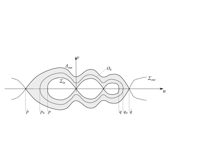
Figure 1: The inner chain and outer loop associated with a connected component $\Pi$ of ${\mathcal{P}}_{0}$: $\Pi$ is indicated by the shaded region, $\Lambda_{out}$ and $\Sigma_{in}$ form the boundary of $\Pi$. The outer loop can be a heteroclinic loop (as in this figure) or a homoclinic loop.

Proof of Lemma 2.7.

The openness of $\Pi$ follows from the compactness of $\mathbb{R}^{2}\setminus\mathcal{P}_{0}$, as already mentioned above. This takes care of statement (i).

In the rest of the proof, we assume for definiteness that $\Pi$ is bounded and prove statements (ii)-(v). The proof of statements (ii), (iv), (v) in the case that $\Pi$ is the unique unbounded connected component of $\mathcal{P}_{0}$ is similar and is omitted.

Fix any periodic orbit $\mathcal{O}_{0}\subset\Pi.$ By (2.5), there are $p_{0}<q_{0}$ such that $\mathcal{O}_{0}\cap\{(u,0):u\in\mathbb{R}\}=\{(p_{0},0),(q_{0},0)\},$ with $f(p_{0})=F^{\prime}(p_{0})<0$ and $f(q_{0})=F^{\prime}(q_{0})>0.$ Define

$$q:=\sup\{q<q_{0}:(q,0)\not\in\Pi\},\ \textrm{ and }\ \hat{q}:=\inf\{q>q_{0}:(q,0)\not\in\Pi\}.$$

In other words, $(q,\hat{q})$ is the maximal open interval containing $q_{0}$ such that $(q,\hat{q})\times\{0\}\subset\Pi$. The existence of such an interval is guaranteed by the openness of $\Pi$. Note also that none of the points $(q,0)$, $(\hat{q},0)$ is contained in ${\mathcal{P}}_{0}$. Indeed, if, say, $(q,0)\in{\mathcal{P}}_{0}$, then a neighborhood of $(q,0)$ is contained in ${\mathcal{P}}_{0}$. By the definition of $q$, this whole neighborhood would necessarily be contained in the connected component $\Pi$, from which we immediately get a contraction to the definition of $q$. So, indeed, $(q,0),(\hat{q},0)\not\in{\mathcal{P}}_{0}$, in particular they are not equilibria of (2.3). Since there is no element of $\mathcal{E}$ in $(q,\hat{q})\times\{0\}\subset\Pi$, we have $F^{\prime}=f\neq 0$ on $(q,\hat{q})$ and $F^{\prime}(q_{0})>0$ implies that $F^{\prime}>0$ on $(q,\hat{q})$. In an analogous way, one finds a maximal interval $(\hat{p},p)$ containing $p_{0}$ such that $(\hat{p},p)\times\{0\}\subset\Pi$, and proves that $(p,0),(\hat{p},0)\not\in{\mathcal{P}}_{0}$ and $F^{\prime}<0$ on $(\hat{p},p)$. A continuity argument shows that the union of all (periodic) orbits of (2.3) intersecting the segment $(q,\hat{q})\times\{0\}$ is equal to the union of all orbits of (2.3) intersecting $(\hat{p},p)\times\{0\}$. We denote this union by $\tilde{\Pi}$. As distinct orbits of (2.3) do not intersect, it is clear that the periodic orbits contained in $\tilde{\Pi}$ are nested in the sense that (v) holds with $\Pi$ replaced by $\tilde{\Pi}$. (We will prove below that in fact $\Pi=\tilde{\Pi}$, thereby proving statement (v).) Observe also that the points $(p,0)$, $(q,0)$ can be approximated arbitrarily closely by one orbit contained in $\tilde{\Pi}$. This implies that they are in the same level set of the Hamiltonian, that is, $F(p)=F(q)$, and also that $F\leq F(q)$ in $(p,q)$. One easily proves from this that the points $(p,0)$, $(q,0)$ lie on the same chain which we denote by $\Sigma_{in}$. Using Lemma 2.6 (and the fact that $(p,0)$, $(q,0)$ are not equilibria), we can write:

$$\Sigma_{in}=\left\{(u,v)\in\mathbb{R}^{2}:u\in[p,q],\ v=\pm\sqrt{2(F(q)-F(u))}\right\}.$$ (2.6)

Similarly one shows that $F(\hat{p})=F(\hat{q})$, $F\leq F(\hat{q})$ in $(\hat{p},\hat{q})$, and the points $(\hat{p},0)$, $(\hat{q},0)$ lie on the same chain, which we denote by $\Sigma_{out}$. By Lemma 2.6,

$$\Sigma_{out}=\left\{(u,v)\in\mathbb{R}^{2}:u\in[\bar{p},\bar{q}],\ v=\pm\sqrt{2(F(\hat{q})-F(u))}\right\}$$

for some $\bar{p}\leq\hat{p}$, $\bar{q}\geq\hat{q}.$ The inequality for $F$ actually holds in the strict sense: $F<F(\hat{q})$ in $(\hat{p},\hat{q})$, due to the previously established relation $F\leq F(q)$ in $(p,q)$ and the strict monotonicity properties of $F$ in the intervals $(\hat{p},p)$, $(q,\hat{q})$. It follows that the set

$$\Lambda_{out}:=\left\{(u,v)\in\mathbb{R}^{2}:u\in[\hat{p},\hat{q}],\ v=\pm\sqrt{2(F(\hat{q})-F(u))}\right\}$$ (2.7)

is a loop contained in $\Sigma_{out}.$ Clearly, $\Sigma_{in}$, $\Sigma_{out}$ are distinct (hence disjoint) chains; in fact, they lie on two different level sets of the Hamiltonian $H$.

It is obvious from the above constructions that for any periodic orbit ${\mathcal{O}}\subset\tilde{\Pi}$ we have

$${\overline{\mathcal{I}}\left(\Sigma_{in}\right)}\subset\mathcal{I}(\mathcal{O})\subset\overline{\mathcal{I}}(\mathcal{O})\subset\mathcal{I}(\Lambda_{out}).$$ (2.8)

We next claim that

$$\mathcal{I}(\Lambda_{out})\setminus\overline{\mathcal{I}}\left(\Sigma_{in}\right)=\tilde{\Pi}.$$ (2.9)

That $\tilde{\Pi}$ is included in the set on the left has already been proved (cp. (2.8)); we prove the opposite inclusion. Take any $(\xi,\eta)\in\mathcal{I}(\Lambda_{out})\setminus\overline{\mathcal{I}}\left(\Sigma_{in}\right)$. If $(\xi,\eta)$ lies on a periodic orbit, then that orbit intersects the $u$-axis in the set $((q,\hat{q})\cup(\hat{p},p))\times\{0\}$ (otherwise, in view of (2.6), (2.7) it would have to intersect one of the chain $\Sigma_{in}$, $\Sigma_{out}$, which is impossible), and hence $(\xi,\eta)\in\tilde{\Pi}$. If $(\xi,\eta)$ does not lie on a periodic orbit, then it is contained in a chain disjoint from $\Sigma_{in}\cup\Sigma_{out}$, and such a chain would also have to intersect the set $((q,\hat{q})\cup(\hat{p},p))\times\{0\}$. This is impossible, as this set is included in $\tilde{\Pi}\subset{\mathcal{P}}_{0}$. Thus (2.9) is true.

From (2.9) it follows that $\tilde{\Pi}$ is a connected component of ${\mathcal{P}}_{0}$, hence $\tilde{\Pi}=\Pi$. As already noted above, this proves statement (v). Statements (iii) and (iv) follow from (2.8), (2.9). To prove statement (iv), take the minimum point $\beta$ of $F$ in $[p,q]$. Recalling that $F^{\prime}(p)<0$, $F^{\prime}(q)>0$, we see that $\beta\in(p,q)$ and it is a local minimum point of $F$, hence $f(\beta)=0$ and $f^{\prime}(\beta)>0$, due to (ND). Statement (v) clearly holds for this $\beta$. ∎

The following lemma shows a relation between any two distinct chains.

Lemma 2.8.

• If $\Sigma$ is any chain, then there is a connected component $\Pi$ of ${\mathcal{P}}_{0}$ such that $\Sigma$ is the inner chain associated with $\Pi$: $\Sigma=\Sigma_{in}(\Pi)$.

• If $\Sigma_{1}$, $\Sigma_{2}$ are any two distinct chains, then either $\Sigma_{1}\subset\mathcal{I}(\Sigma_{2})$, or $\Sigma_{2}\subset\mathcal{I}(\Sigma_{1})$, or else there are periodic orbits ${\mathcal{O}}_{1}$, ${\mathcal{O}}_{2}$ such that $\overline{{\mathcal{I}}}({\mathcal{O}}_{1})\cap\overline{{\mathcal{I}}}({\mathcal{O}}_{2})=\emptyset$ and

  $$\Sigma_{1}\subset\mathcal{I}({\mathcal{O}}_{1}),\qquad\Sigma_{2}\subset\mathcal{I}({\mathcal{O}}_{2}).$$ (2.10)

Proof.

Since there are only finitely many chains, for any given chain $\Sigma$ there is a connected component $\Pi$ of ${\mathcal{P}}_{0}$ such that $\Pi\subset\mathbb{R}^{2}\setminus\overline{\mathcal{I}}(\Sigma)$ and the boundary of $\Pi$ contains points of $\Sigma$. It then follows from Lemma 2.7 that $\Sigma=\Sigma_{in}(\Pi)$. This proves statement (i).

Let now $\Sigma_{1}$, $\Sigma_{2}$ be any two distinct chains, and let $\Pi_{1}$, $\Pi_{2}$ be the connected components of ${\mathcal{P}}_{0}$ such that $\Sigma_{j}=\Sigma_{in}(\Pi_{i})$, $j=1,2$. Pick periodic orbits ${\mathcal{O}}_{1}\subset\Pi_{1}$, ${\mathcal{O}}_{2}\subset\Pi_{2}$. By Lemma 2.7, inclusions (2.10) hold. Clearly, exactly one of the following possibilities occurs:

$${\rm(a)}\quad{\mathcal{O}}_{1}\subset\mathcal{I}({\mathcal{O}}_{2}),\qquad{\rm(b)}\quad{\mathcal{O}}_{2}\subset\mathcal{I}({\mathcal{O}}_{1})\qquad{\rm(c)}\quad\overline{{\mathcal{I}}}({\mathcal{O}}_{1})\cap\overline{{\mathcal{I}}}({\mathcal{O}}_{2})=\emptyset.$$

For the proof of statement (ii), it is now sufficient to prove that (a) implies that $\Sigma_{1}\subset\mathcal{I}(\Sigma_{2})$, and (b) implies $\Sigma_{2}\subset\mathcal{I}(\Sigma_{1})$. These being symmetrical cases, we only prove the former. Trivially, $\Sigma_{1}\cap(\Pi_{2}\cup\Sigma_{2})=\emptyset$; and Lemma 2.7(ii) gives $\mathcal{I}(\mathcal{O}_{2})\setminus{\overline{\mathcal{I}}(\Sigma_{2})}\subset\Pi_{2}$. Thus, if (a) holds, which entails $\Sigma_{1}\subset\mathcal{I}({\mathcal{O}}_{2})$, then necessarily $\Sigma_{1}\subset\mathcal{I}(\Sigma_{2})$. ∎

2.3 Limit sets and entire solutions

Recall that the $\omega-$limit set of a bounded solution $u$ of (1.1), denoted by $\omega(u)$, or $\omega(u_{0})$ if the initial value of $u$ is given, is defined as in (1.4), with the convergence in $L^{\infty}_{loc}(\mathbb{R})$. By standard parabolic estimates the trajectory $\{u(\cdot,t),\ t\geq 1\}$ of $u$ is relatively compact in $L^{\infty}_{loc}(\mathbb{R}).$ This implies that $\omega(u)$ is nonempty, compact, and connected in (the metric space) $L^{\infty}_{loc}(\mathbb{R})$ and it attracts the solution in the following sense:

$$\textrm{dist}_{L^{\infty}_{loc}(\mathbb{R})}\left(u(\cdot,t),\omega(u)\right)\underset{t\to\infty}{\longrightarrow}0.$$ (2.11)

It is also a standard observation that if $\varphi\in\omega(u),$ there exists an entire solution $U(x,t)$ of (1.1), that is, a solution defined for all $t\in\mathbb{R}$, such that

$$U(\cdot,0)=\varphi,\qquad U(\cdot,t)\in\omega(u)\quad(t\in\mathbb{R}).$$ (2.12)

We recall briefly how such an entire solution $U$ is found. By parabolic regularity estimates, $u_{t},u_{x},u_{xx}$ are bounded on $\mathbb{R}\times[1,\infty)$ and are globally $\alpha-$Hölder for any $\alpha\in(0,1).$ If $u(\cdot,t_{n})\underset{n\to\infty}{\longrightarrow}\varphi$ in $L^{\infty}_{loc}(\mathbb{R})$ for some $t_{n}\to\infty,$ we consider the sequence $u_{n}(x,t):=u(x,t+t_{n})$, $n=1,2\dots$. Passing to a subsequence if necessary, we have $u_{n}\to U$ in $C^{1}_{loc}(\mathbb{R}^{2})$ for some function $U;$ this function $U$ is then easily shown to be an entire solution of (1.1). By definition, $U$ satisfies (2.12). Note that the entire solution $U$ is determined uniquely by $\varphi$; this follows from the uniqueness and backward uniqueness for the Cauchy problem (1.1), (1.2).

Using similar compactness arguments, one shows easily that $\omega(u)$ is connected in $C_{loc}^{1}(\mathbb{R}).$ Hence, the set

$$\tau\left(\omega(u)\right)=\left\{(\varphi(x),\varphi_{x}(x)):\varphi\in\omega(u),x\in\mathbb{R}\right\}=\underset{\varphi\in\omega(u)}{\textstyle\bigcup}\tau(\varphi)$$

is connected in $\mathbb{R}^{2}$. (Here, $\tau(\varphi)$ is as in (1.10).) Also, obviously, $\tau(\varphi)$ is connected in $\mathbb{R}^{2}$ for all $\varphi\in\omega(u).$

If $U$ is a bounded entire solution of (1.1), we define its $\alpha-$limit set by

$$\alpha(U):=\left\{\varphi\in C_{b}(\mathbb{R}):U(\cdot,t_{n})\to\varphi\textrm{ for some sequence }t_{n}\to-\infty\right\}.$$ (2.13)

Here, again, the convergence is in $L_{loc}^{\infty}(\mathbb{R}).$ The $\alpha$-limit set has similar properties as the $\omega-$limit set: it is nonempty, compact and connected in $L^{\infty}_{loc}(\mathbb{R})$ as well as in $C^{1}_{loc}(\mathbb{R})$, and for any $\varphi\in\alpha(U)$ there is an entire solution $\tilde{U}$ such that $\tilde{U}(\cdot,0)=\varphi$ and $\tilde{U}(\cdot,t)\in\alpha(U)$ for all $t\in\mathbb{R}$. The connectivity property of $\alpha(U)$ implies that the set

$$\tau\left(\alpha(U)\right)=\left\{(\varphi(x),\varphi_{x}(x)):\varphi\in\alpha(U),x\in\mathbb{R}\right\}=\underset{\varphi\in\alpha(U)}{\textstyle\bigcup}\tau(\varphi)$$

is connected in $\mathbb{R}^{2}.$

We will also employ a generalized notion of $\alpha$ and $\omega$-limit sets. Namely, if $U$ is a bounded entire solution, we define

$$\Omega(U) :=\left\{\varphi\in C_{b}(\mathbb{R}):U(\cdot+x_{n},t_{n})\to\varphi\textrm{ for some sequences }x_{n}\in\mathbb{R},\ t_{n}\to\infty\right\},$$ (2.14)

$$A(U) :=\left\{\varphi\in C_{b}(\mathbb{R}):U(\cdot+x_{n},t_{n})\to\varphi\textrm{ for some sequences }x_{n}\in\mathbb{R},\ t_{n}\to-\infty\right\}.$$ (2.15)

The convergence is in $L_{loc}^{\infty}(\mathbb{R})$, but again one can take the convergence in $C^{1}_{loc}(\mathbb{R})$ without altering the sets $\Omega(U)$, $A(U)$. These sets are nonempty, compact and connected in $C^{1}_{loc}(\mathbb{R})$, and they have a similar invariance property as $\omega(u)$ (cp. (2.12)). Also, by their definitions, the sets $\Omega(U)$, $A(U)$ are translation invariant as well. Further, the definitions and parabolic regularity imply that the sets

$$\tau\left(A(U)\right)=\underset{\varphi\in A(U)}{\textstyle\bigcup}\tau(\varphi),\quad\tau\left(\Omega(U)\right)=\underset{\varphi\in\Omega(U)}{\textstyle\bigcup}\tau(\varphi)$$

are connected and compact in $\mathbb{R}^{2}.$ We remark that the sets $\tau(\omega(u))$, $\tau(\alpha(u))$ are both connected (as noted above), but they are not necessarily compact in $\mathbb{R}^{2}$.

2.4 Some results from earlier papers

Several earlier results are used repeatedly in the forthcoming sections. We state them here for reference.

Throughout this subsection, we assume that $u_{0}\in C_{b}(\mathbb{R})$ (not necessarily in ${\mathcal{V}}$), $u$ is the solution of (1.1), (1.2) and it is bounded.

In view of the invariance property of $\omega(u)$ (see (2.12)), the following lemma gives a criterion for an element $\varphi\in\omega(u)$ to be a steady state. This unique-continuation type result is proved in a more general form in [35, Lemma 6.10].

Lemma 2.9.

Let $\varphi:=U(\cdot,0)$, where $U$ is a solution of (1.1) defined on a time interval $(-\delta,\delta)$ with $\delta>0$ (this holds in particular if $\varphi\in\omega(u)$). If $\tau(\varphi)\subset\Sigma$ for some chain $\Sigma,$ then $\varphi$ is a steady state of (1.1).

As already noted above, it is proved in [18] (see also [19]) that the $\omega$-limit set of any bounded solution of (1.1) contains a steady state. For bounded entire solutions $U$, the same is true for the $\alpha$-limit set due to its compactness and invariance properties (just apply the previous result to any entire solution $\tilde{U}$ with $\tilde{U}(\cdot,t)\in\alpha(U)$). We state this in the following theorem.

Theorem 2.10.

If $U$ is a bounded entire solution of (1.1), then each of the sets $\omega(U)$ and $\alpha(U)$ contains a steady state of (1.1).

In the next two results, we make use of the invariance of equation (1.1) under spatial reflections. For any $\lambda\in\mathbb{R}$ consider the function $V_{\lambda}u$ defined by

$$V_{\lambda}u(x,t)=u(2\lambda-x,t)-u(x,t),\quad x\in\mathbb{R},\,t\geq 0.$$ (2.16)

Being the difference of two solutions of (1.1), $V_{\lambda}u$ is a solution of the linear equation (2.1) for some bounded function $c.$

The following lemma is an adaptation of an argument from [2, Proof of Proposition 2.1].

Lemma 2.11.

Let $U$ be a solution of (1.1) on $\mathbb{R}\times J$, where $J\subset\mathbb{R}$ is an open time interval, and let $\theta\in\mathbb{R}$. Assume that for each $t\in J$ the function $U(\cdot,t)-\theta$ has at least one zero and

$$\xi(t):=\sup\{x:U(x,t)=\theta\}$$

is finite and depends continuously on $t\in J$. Then, for any $t_{0},t_{1}\in J$ satisfying the relations $t_{1}>t_{0}$ and $\xi(t_{1})<\xi(t_{0})$, the function $U_{x}(\cdot,t_{1})$ is of constant sign on the interval $(\xi(t_{1}),\xi(t_{0})]$. If $J=(-\infty,b)$ for some $-\infty<b\leq\infty$ and $\limsup_{t\to-\infty}\xi(t)=\infty$, then $U_{x}$ is of constant sign on $(\xi(t),\infty),$ for all $t\in J.$

Analogous statements hold for $\xi(t)=\inf\{x:U(x,t)=\theta\}.$

Proof.

Pick any $\lambda\in(\xi(t_{1}),\xi(t_{0})]$ and set $\displaystyle\bar{t}:=\max\left\{t\in[t_{0},t_{1}):\xi(t)=\lambda\right\}$. Consider the function $V_{\lambda}U$ on the domain

$$Q_{\lambda}:=\left\{(x,t):\ x\in(\xi(t),\lambda),\ t\in(\bar{t},t_{1})\right\}.$$

Clearly, $V_{\lambda}U(\lambda,t)=0$ for all $t$ and, as $\xi(t)$ is the last zero of $U(\cdot,t)$, $V_{\lambda}U(\xi(t),t)$ is of constant sign on $(t_{0},t_{1})$. Since $V_{\lambda}U$ solves a linear parabolic equation (2.1), the maximum principle implies that $V_{\lambda}U$ is of constant sign on the whole domain $Q_{\lambda}$, and the Hopf lemma yields $-2\partial_{x}U(\lambda,t_{1})=\partial_{x}V_{\lambda}u(\lambda,t_{1})\neq 0$. Since $\lambda\in(\xi(t_{1}),\xi(t_{0})]$ was arbitrary, $U_{x}(\cdot,t_{1})$ is of constant sign on $(\xi(t_{1}),\xi(t_{0})]$.

To prove the second statement, fix any $t^{\prime}\in J$ and let $\lambda>\xi(t^{\prime})$. By the unboundedness assumption on $\xi(t)$, $t_{0}:=\sup\{t<t^{\prime}:\xi(t)=\lambda\}$ is a number in $(-\infty,t^{\prime})$. Applying the result just proved, we obtain $U_{x}(\lambda,t^{\prime})\neq 0$. Since $\lambda>\xi(t^{\prime})$ was arbitrary, we obtain the desired conclusion. ∎

We next state a quasiconvergence result from our previous paper [29].

Theorem 2.12.

Assume that $u_{0}\in{\mathcal{V}}$ and one of the following conditions holds:

• $u_{0}(-\infty)\neq u_{0}(\infty)$,

• there is $t>0$ such that for all $\lambda\in\mathbb{R},$ one has $z(V_{\lambda}u(\cdot,t))<\infty.$

Then, $u$ is quasiconvergent.

If condition (i) is assumed, this is the content of the main theorem in [29]. In the proof of the theorem, we first proved that condition (i) and Lemma 2.1 imply that condition (ii) holds (this is actually the only place where condition (i) is used in the proof). As noted in [29, Remark 3.3], the quasiconvergence result holds if condition (i) is replaced by (ii) from the start.

The following result concerning various invariant sets for (1.1) is a variant of the squeezing lemma from [34]. This is an indispensable tool in our proofs.

Lemma 2.13.

Let $U$ be a bounded entire solution of (1.1) such that if $\beta\in f^{-1}\{0\}$ is an unstable equilibrium of (1.7), then

$$z\left(U(\cdot,t)-\beta\right)\leq N\quad(t\in\mathbb{R})$$ (2.17)

for some $N<\infty.$ Let $K$ be any one of the following subsets of $\mathbb{R}^{2}:$

$$\underset{t\in\mathbb{R}}{{\textstyle\bigcup}}\tau\left(U(\cdot,t)\right),\quad\tau\left(\omega(U)\right),\quad\tau\left(\Omega(U)\right),\quad\tau\left(\alpha(U)\right),\quad\tau\left(A(U)\right).$$

Assume that $\mathcal{O}$ is a non-stationary periodic orbit of (2.3) such that one of the following inclusions holds:

(i)  $$K\subset\mathcal{I}(\mathcal{O}) K\subset\mathbb{R}^{2}\setminus{\overline{\mathcal{I}}(\mathcal{O})}$$,    (ii) .

Let $\Pi$ be the connected component of ${\mathcal{P}}_{0}$ containing ${\mathcal{O}}$. If (i) holds, then $K\subset{\overline{\mathcal{I}}\left(\Sigma_{in}(\Pi)\right)}$; and if (ii) holds, then $K\subset\mathbb{R}^{2}\setminus\mathcal{I}\left(\Lambda_{out}(\Pi)\right)$ (in particular, $\Pi$ is necessarily bounded in this case).

Proof.

We prove the result in the case (i) only, the proof in the case (ii) is analogous. To simplify the notation, let $\Sigma_{in}:=\Sigma_{in}(\Pi)$.

Take first $\displaystyle K={\textstyle\bigcup}_{t\in\mathbb{R}}\tau\left(U(\cdot,t)\right)$. We go by contradiction: assume that $K\not\subset{\overline{\mathcal{I}}\left(\Sigma_{in}\right)}.$ Then there exists a periodic orbit $\mathcal{O}_{1}\subset\Pi$ such that $\displaystyle\tau\left(U(\cdot,t_{1})\right)\cap\mathcal{O}_{1}\neq\emptyset,$ for some $t_{1}\in\mathbb{R}.$ By the hypotheses, $\overline{K}\subset\overline{\mathcal{I}}(\mathcal{O})$ and $\overline{K}$ is a compact set. Using the compactness and the ordering of periodic orbits contained in $\Pi,$ as given in Lemma 2.7(v), we find the minimal periodic orbit $\mathcal{O}_{min}\subset\mathcal{P}_{0}$ with $\overline{K}\subset{\overline{\mathcal{I}}\left(\mathcal{O}_{min}\right)}$. Clearly,

$$\overline{K}\subset{\overline{\mathcal{I}}\left(\mathcal{O}_{min}\right)},\qquad\overline{K}\cap\mathcal{O}_{min}\neq\emptyset.$$ (2.18)

Hence, there exist sequences $x_{n},t_{n}$ such that

$$\left(U(x_{n},t_{n}),U_{x}(x_{n},t_{n})\right)\underset{n\to\infty}{\longrightarrow}(a,b)\in\mathcal{O}_{min}.$$

Let $\psi_{min}$ be a periodic solution of (1.6) with $\psi_{min}(0)=a,$ $\psi_{min}^{\prime}(0)=b,$ so that $\tau(\psi_{min})=\mathcal{O}_{min}.$ Consider the sequence of functions $U_{n}:=U(\cdot+x_{n},\cdot+t_{n}).$ By parabolic estimates, upon extracting a subsequence, $U_{n}$ converges in $C^{1}_{loc}(\mathbb{R}^{2})$ to an entire solution $U_{\infty}$ of (1.1). Obviously, $U_{\infty}(\cdot,0)-\psi_{min}$ has a multiple zero at $x=0.$

We claim that $U_{\infty}\not\equiv\psi_{min}.$ Indeed, by Lemma 2.7(iv), there exists an unstable equilibrium $\beta$ of (1.7) such that $\displaystyle z(\psi_{min}-\beta)=\infty.$ Hence, there exists $M>0$ such that $\displaystyle z_{(-M,M)}(\psi_{min}-\beta)>N+1,$ where $N$ is as in (2.17). Obviously, all zeros of $\psi_{min}-\beta$ are simple. Considering that $U(\cdot+x_{n},t_{n})$ converges uniformly on $(-M,M)$ to $U_{\infty}(\cdot,0)$ and $\displaystyle z_{(-M,M)}\left(U(\cdot+x_{n},t_{n})-\beta\right)\leq N,$ we see that $U_{\infty}$ cannot be identical to $\psi_{min}.$

Now, using Lemma 2.7(v), we find a sequence $\mathcal{O}_{n}$ of periodic orbits such that $\displaystyle\mathcal{O}_{n+1}\subset\mathcal{I}\left(\mathcal{O}_{n}\right)$, $\displaystyle\mathcal{O}\subset\mathcal{I}\left(\mathcal{O}_{n}\right)$, for $n=1,2,\dots$, and $\displaystyle\operatorname{dist}\left(\mathcal{O}_{n},\mathcal{O}_{min}\right)\to 0.$ There is a sequence $\psi_{n}$ of periodic solutions of (1.6) such that $\tau(\psi_{n})={\mathcal{O}}_{n}$ and $\displaystyle\psi_{n}\to\psi_{min}$ in $C^{1}_{loc}(\mathbb{R}).$ Then, the sequence of functions $w_{n}:=U_{n}-\psi_{n}$ converges in $C^{1}_{loc}(\mathbb{R}^{2})$ to $w(x,t):=U_{\infty}(x,t)-\psi_{min}(x)$, which is an entire solution of a linear parabolic equation (2.1). Since $w(\cdot,0)$ has a multiple zero at $x=0$ and $w(\cdot,0)\not\equiv 0,$ Lemma 2.5 implies that there exist $n_{0},x_{0},\delta_{0}$ such that the function $w_{n_{0}}(\cdot,\delta_{0})$ has a multiple zero at $x=x_{0}.$ Consequently,

$$\tau\left(U(\cdot,t_{n_{0}}+\delta_{0})\right)\cap\mathcal{O}_{n_{0}}\neq\emptyset.$$ (2.19)

However, since $\mathcal{O}_{min}\subset\mathcal{I}({O}_{n_{0}}),$ (2.19) contradicts (2.18). This contradiction concludes the proof of Lemma 2.13 in the case $\displaystyle K=\underset{t\in\mathbb{R}}{\cup}\tau\left(U(\cdot,t)\right)$.

If $K$ is any of the sets $\tau\left(\omega(U)\right)$, $\tau\left(\Omega(U)\right)$, $\tau\left(\alpha(U)\right)$, $\tau\left(A(U)\right)$, then the conclusion follows from the previous case and the invariance properties of these sets. Indeed, consider $K=\tau\left(\omega(U)\right)$ for instance, the other cases being similar. For any $\varphi\in\omega(U)$ there is an entire solution $\tilde{U}$ with $\tilde{U}(\cdot,t)\in\omega(U)$ for all $t$ and $\tilde{U}(\cdot,0)=\varphi.$ Then $\displaystyle\tilde{K}:=\underset{t\in\mathbb{R}}{\cup}\tau\left(\tilde{U}(\cdot,t)\right)$ satisfies the hypotheses of the first case, and so $\tilde{K}$ is included in ${\overline{\mathcal{I}}\left(\Sigma_{in}\right)}.$ This is true for all $\varphi\in\omega(U),$ hence $\displaystyle\tau\left(\omega(U)\right)\subset{\overline{\mathcal{I}}\left(\Sigma_{in}\right)}.$ ∎

Finally, we recall the following well known result concerning the solutions in ${\mathcal{V}}$ (the proof can be found in [38, Theorem 5.5.2], for example).

Lemma 2.14.

Assume that $u_{0}\in{\mathcal{V}}$. Then the limits

$$\theta_{-}(t):=\lim_{x\to-\infty}u(x,t),\qquad\theta_{+}(t):=\lim_{x\to\infty}u(x,t)$$ (2.20)

exist for all $t>0$ and are solutions of the following initial-value problems:

$$\dot{\theta}_{\pm}=f(\theta_{\pm}),\qquad\theta_{\pm}(0)=u_{0}(\pm\infty).$$ (2.21)

3 Spatial trajectories of entire solutions in $\omega(u)$

Throughout this section, we assume, in addition to the standing hypotheses (ND), (MF) on $f$, that $u_{0}\in{\mathcal{V}}$, $u_{0}(\pm\infty)=0$, and the solution of (1.1), (1.2) is bounded. We reserve the symbol $u(x,t)$ for this fixed solution.

Due to (2.21), the limits (2.20) are equal: $\theta^{+}\equiv\theta^{-}=:\hat{\theta}$, where $\hat{\theta}$ is the solution of (1.7) with $\hat{\theta}(0)\equiv 0$. This gives the first two statements of the following corollary; the last statement follows from Lemma 2.1.

Corollary 3.1.

If $f(0)=0$, then $\hat{\theta}\equiv 0$; we set $\theta:=0$ in this case. If $f(0)\neq 0$, then $\hat{\theta}(t)\to\theta\in\mathbb{R}$ as ${t\to\infty}$, where $\theta\in f^{-1}\{0\}$ is a stable equilibrium of (1.7). In either case, if $\psi$ is any periodic steady state of (1.6) such that $\theta$ is not in the range of $\psi,$ then there exists $T>0$ such that $\displaystyle z(u(\cdot,t)-\psi)<\infty$ for all $t>T.$

Following the outline given in Section 1.4, we examine the elements $\varphi$ of $\omega(u)$ whose spatial trajectories are not contained in any chain. At the end, we want to show that no such elements of $\omega(u)$ exist (an application of Lemma 2.9 then yields the desired quasiconvergence results). For that aim, we first examine the entire solutions through such elements $\varphi\in\omega(u)$. In Proposition 3.2 below, we expose a certain structure these entire solutions would necessarily have to have. Then, in Section 6, we show that that structure is incompatible with other properties of the $\omega$-limit set.

Up to a point, we treat the cases (S) and (U) simultaneously. When (U) holds, we sometimes have to assume one or both of the extra conditions (NC), (R); we indicate when this is needed. The following notation will be used in the case (U): $\Pi_{0}$ is the connected component of $\mathcal{P}_{0}$ whose closure contains $(0,0)$. Note that $\Pi_{0}$ is well defined, for $f^{\prime}(0)>0$ implies that $(0,0)$ is a center for (2.3).

Proposition 3.2.

Under the above hypotheses, assume that $\varphi\in\omega(u)$ and let $U$ be the entire solution of (1.1) with $U(\cdot,0)=\varphi.$ Assume that $\tau(\varphi)\cap\mathcal{P}_{0}\neq\emptyset$, so that there exists a connected component $\Pi$ of $\mathcal{P}_{0}$ with

$$\tau(\varphi)\cap\Pi\neq\emptyset.$$ (3.1)

If (S) holds, or if (U) holds and $\Pi\neq\Pi_{0}$, then the following statements are true.

• The connected component $\Pi$ satisfying (3.1) is unique, it is bounded, and

  $$\underset{t\in\mathbb{R}}{{\textstyle\bigcup}}\tau\left(U(\cdot,t)\right)\subset\Pi.$$ (3.2)

• Let $\Sigma_{in}=\Sigma_{in}(\Pi)$ be the inner chain and $\Lambda_{out}=\Lambda_{out}(\Pi)$ the outer loop associated with $\Pi,$ as in Lemma 2.7. Then

  $$\tau\left(\alpha(U)\right)\subset\Sigma_{in},\qquad\tau\left(\omega(U)\right)\subset\Lambda_{out}.$$ (3.3)

If (U) holds and $\Pi=\Pi_{0}$, then statement (i) is true if condition (NC) is satisfied, and statement (ii) is true if conditions (NC) and (R) are both satisfied.

Statement (i) is proved in the next subsection. Subsection 3.2 is devoted to the behavior at $x\approx\pm\infty$ of $U(\cdot,t),$ and subsection 3.3 to additional properties when (U) holds. Statement (ii) is then proved in sections 4 and 5.

For the remainder of this section, we fix $\varphi\in\omega(u)$ and denote by $U$ be the entire solution of (1.1) such that $U(\cdot,0)=\varphi$ and $U(\cdot,t)\in\omega(u)$ for all $t.$ Recall from Section 2.3 that there exists a sequence $t_{n}\to\infty$ such that

$$u(\cdot,\cdot+t_{n})\underset{n\to\infty}{\longrightarrow}U\textrm{ in }C_{loc}^{1}(\mathbb{R}^{2}).$$ (3.4)

3.1 No intersection with chains

In this subsection, we prove statement (i) of Proposition 3.2. The following result is a first step toward that goal.

Lemma 3.3.

Let $\Sigma\subset\mathbb{R}^{2}$ be a nontrivial chain. If $\tau(\varphi)\cap\mathcal{I}(\Sigma)\neq\emptyset$, then

$$\tau(U(\cdot,t))\subset\mathcal{I}(\Sigma)\quad(t\in\mathbb{R})$$ (3.5)

(in particular, $\tau(U(\cdot,t))\cap\Sigma=\emptyset$ for all $t\in\mathbb{R}$). The result remains valid if one considers a loop $\Lambda$ in place of the chain $\Sigma.$

Proof.

Note that the second statement is a consequence of the first one; just consider the chain $\Sigma$ containing the loop $\Lambda$ and use the connectedness of the set $\cup_{t\in\mathbb{R}}\tau(U(\cdot,t))$.

Let $\Sigma$ be a nontrivial chain. We first show that the assumption $\tau(\varphi)\cap\mathcal{I}(\Sigma)\neq\emptyset$ implies

$$\tau(\varphi)\cap\Sigma=\emptyset.$$ (3.6)

Assume for a contradiction that the intersections are both nonempty. The relation $\tau(\varphi)\cap\Sigma\neq\emptyset$ means that there is a steady state $\phi$ of (1.1) such that $\tau(\phi)\subset\Sigma$ and $U(\cdot,0)-\phi=\varphi-\phi$ has a multiple zero at some point $x_{0}$. Using both assumptions $\tau(\varphi)\cap\Sigma\neq\emptyset$ and $\tau(\varphi)\cap\mathcal{I}(\Sigma)\neq\emptyset$, together with the connectedness of $\tau(\varphi)$ and the fact that distinct chains are disjoint with positive distance, we find a periodic orbit $\mathcal{O}\subset\mathcal{P}_{0}\cap\mathcal{I}(\Sigma)$ such that $\tau(U(\cdot,0))\cap\mathcal{O}\neq\emptyset.$ Hence there is a steady state $\psi$ of (1.1) such that $\tau(\psi)=\mathcal{O}$ (so $\psi$ is nonconstant and periodic) and $U(\cdot,0)-\psi=\varphi-\psi$ has a multiple zero at some $x_{1}.$ Obviously, $U(\cdot,0)-\phi\not\equiv 0\not\equiv U(\cdot,0)-\psi$.

From $\tau(\phi)\subset\Sigma$, we infer that $\phi$ is either a ground state at some level $a\in f^{-1}\{0\}$, or a standing wave with some limits $a,b\in f^{-1}\{0\}$, or a constant steady state $a$. We just consider the first possibility, the other two being similar. Assuming that $\phi$ is a ground state at level $a,$ we first show that necessarily $a=0$ (and consequently $0$ is a stable equilibrium of (1.7), cp. Sect. 2.2). Indeed, the function $w(x,t)=U(x,t)-\phi(x)$ is a nontrivial solution of a linear equation (2.1) and $w(\cdot,0)$ has a multiple zero at $x=x_{0}.$ By (3.4), the sequence $w_{n}:=u(\cdot,\cdot+t_{n})-\phi$ converges in $C^{1}_{loc}(\mathbb{R}^{2})$ to $w.$ Therefore, by Lemma 2.5, there exist sequences $x_{n}\to x_{0},$ $\delta_{n}\to 0$ such that for all sufficiently large $n$ the function $w_{n}(\cdot,\delta_{n})$ has a multiple zero at $x=x_{n}.$ In other words, $u(\cdot,t_{n}+\delta_{n})-\phi$ has a multiple zero at $x=x_{n}.$ Since $t_{n}+\delta_{n}\to\infty$ and $u(\cdot,t)\not\equiv\phi$ (due to the assumption $\tau(\varphi)\cap\mathcal{I}(\Sigma)\neq\emptyset$), Lemma 2.1 implies that $z(u(\cdot,t)-\phi)=\infty$ for all $t>0.$ Now, $\phi(\pm\infty)=a$ and $u(\pm\infty,t)=\hat{\theta}(t)$, where $f(a)=0$ (and $a$ is a stable equilibrium of (1.7)) and $\hat{\theta}$ is a solution of (1.7). If $\hat{\theta}(t)\neq a$ for some (hence any) $t$, then, by Lemma 2.1, $z(u(\cdot,t)-\phi)<\infty$. Thus, necessarily, $\hat{\theta}\equiv a$, which shows that $a=0$, as desired.

To conclude, we use the fact that $(0,0)=(a,0)$ belongs to $\Sigma$, as does $\tau(\phi)$. Since $\Sigma$ is connected and $\tau(\psi)\subset\mathcal{I}(\Sigma),$ we have either $\psi>0$ or $\psi<0.$ Therefore, by Corollary 3.1, $z(u(\cdot,t)-\psi)<\infty$ for all large enough $t$. On the other hand, using Lemma 2.5 in a similar way as above, since $U(\cdot,t_{1})-\psi$ has a multiple zero and $U(\cdot,t_{1})\not\equiv\psi,$ we obtain that $z(u(\cdot,t)-\psi)=\infty$ for all $t>0$. This contradiction completes the proof of (3.6).

Using (3.6), the connectedness of $\tau(\varphi)$, and the assumption $\tau(\varphi)\cap\mathcal{I}(\Sigma)\neq\emptyset$ we obtain that $\tau(\varphi)\subset\mathcal{I}(\Sigma)$. The stronger statement (3.5) follows from this. Indeed, if (3.5) is not valid, then for some $t_{1}$, we have $\tau(U(\cdot,t_{1}))\subset\overline{\mathcal{I}}(\Sigma)$ and $\tau(U(\cdot,t_{1}))\cap\Sigma\neq\emptyset$. At the same time, $\tau(U(\cdot,t_{1}))\not\subset\Sigma$ (otherwise, $U\equiv\varphi$ is a steady state, by Lemma 2.9, and then $\tau(\varphi)\subset\Sigma$ would contradict the assumption). Thus, $\tau(U(\cdot,t_{1}))\cap{\mathcal{I}}(\Sigma)\neq\emptyset$. Applying what we have already proved to $U(\cdot,t_{1})\in\omega(u)$ in place of $\varphi$, we obtain $\tau(U(\cdot,t_{1}))\cap\Sigma=\emptyset$, a contradiction. The proof is now complete. ∎

The next result is analogous to the previous one, but the proof requires different arguments.

Lemma 3.4.

If $\Sigma$ is a nontrivial chain and $\tau(\varphi)\cap(\mathbb{R}^{2}\setminus\overline{\mathcal{I}}\left(\Sigma\right))\neq\emptyset$, then

$$\tau(U(\cdot,t))\subset\mathbb{R}^{2}\setminus\overline{\mathcal{I}}\left(\Sigma\right)\quad(t\in\mathbb{R})$$ (3.7)

(in particular, $\tau(U(\cdot,t))\cap\Sigma=\emptyset$ for all $t\in\mathbb{R}$).

Proof.

It is sufficient to prove that $\tau(\varphi)\cap\Sigma=\emptyset$. The stronger conclusion (3.7) follows from this by a similar argument as in the last paragraph of the previous proof.

We go by contradiction. Assume that $\tau(\varphi)\cap(\mathbb{R}^{2}\setminus\overline{\mathcal{I}}\left(\Sigma\right))\neq\emptyset$ and at the same time $\tau(\varphi)\cap\Sigma\neq\emptyset$. Then, there is a solution $\phi$ of (1.6) with $\tau(\phi)\subset\Sigma$ such that $U(\cdot,0)-\phi=\varphi-\phi$ has a multiple zero at some $x=x_{0}.$ Clearly, $\phi$ is either a ground state, or a standing wave, or a zero of $f$ which is the limit of some ground state or standing wave. In either case, $\tau(\phi)$ is contained in a loop $\Lambda\subset\Sigma$. To derive a contradiction, we choose a sequence $\psi_{n}$ of periodic solutions of (1.6) such that ${\mathcal{O}}_{n}:=\tau(\psi_{n})\subset{\mathcal{I}}(\Lambda)$ and $\psi_{n}\to\phi$ in $C^{1}_{loc}(\mathbb{R})$ (the existence of such a sequence of periodic orbits ${\mathcal{O}}_{n}$ is guaranteed by Lemma 2.7 and the fact that distinct chains are disjoint with positive distance). Then the sequence $w_{n}(x,t):=U(x,t)-\psi_{n}(x)$ converges in $C^{1}_{loc}(\mathbb{R}^{2})$ to $w(x,t):=U(x,t)-\phi,$ a solution of a linear equation (2.1). Since $U(\cdot,0)=\varphi\not\equiv\phi$, we have that $w\not\equiv 0$. Moreover, $w(\cdot,0)$ has a multiple zero at $x=x_{0}.$ Hence, by Lemma 2.5, there exist $n_{1}$, $t_{1}$ such that $w_{n_{1}}(\cdot,t_{1})$ has a multiple zero. This means that $\tau(U(\cdot,t_{1}))\cap\mathcal{O}_{n_{1}}\neq\emptyset$, hence $\tau(U(\cdot,t_{1}))\cap{\mathcal{I}}(\Lambda)\neq\emptyset$. Applying Lemma 3.3 to $U(\cdot,t_{1})$ in place of $\varphi$, and taking $t=0$ in (3.5), we obtain a contradiction to the assumption that $\tau(\varphi)\cap(\mathbb{R}^{2}\setminus\overline{\mathcal{I}}\left(\Sigma_{in}\right))\neq\emptyset$. ∎

In the next lemma, we deal with a trivial chain $\Sigma$, that is, $\Sigma=\{(\beta,0)\}$, where $\beta$ is an unstable equilibrium of (1.7).

Lemma 3.5.

Assume that $\Sigma=\{(\beta,0)\}$ is a trivial chain. If $\beta=0$ (so (U) holds), assume also that condition (NC) is satisfied. Then $(\beta,0)\not\in\tau(\varphi)$, which is the same as $\tau(\varphi)\cap\Sigma=\emptyset$, unless $U\equiv\varphi\equiv\beta=0$.

Proof.

Assume that $(\beta,0)\in\tau(\varphi)$. If $\varphi\not\equiv\beta$, then $U-\beta$ is a nontrivial solution of a linear equation. Hence, by Lemma 2.5, there is a sequence $t_{n}\to\infty$ such that $u(\cdot,t_{n})-\beta$ has a multiple zero for $n=1,2,\dots$. Then by Lemma 2.1,

$$z(u(\cdot,t)-\beta)=\infty\quad(t>0),$$ (3.8)

which is possible only if $u(\pm\infty,t)=\beta$ for all $t>0$. Since $\beta$ is an unstable equilibrium of (1.7), this relation means that (U) holds and $\beta=0$. However, in this situation assumption (NC) is in effect, which clearly contradicts (3.8). This contradiction shows that for $(\beta,0)\in\tau(\varphi)$ it is necessary that $U\equiv\varphi\equiv\beta=0$. ∎

We are ready to complete the proof of Proposition 3.2(i).

Proof of Proposition 3.2(i).

Assume that (3.1) holds for a connected component $\Pi$ of ${\mathcal{P}}_{0}$. We first claim that $\Pi$ is bounded. Suppose not. Since $u(\cdot,t)$ and $u_{x}(\cdot,t)$ are uniformly bounded as $t\to\infty$, using (MF) we find a periodic orbit $\mathcal{O}\subset\Pi$ such that $\displaystyle\tau(U(\cdot,t))\subset\mathcal{I}(\mathcal{O}),$ for all $t\in\mathbb{R}.$ Then Lemma 2.13 implies that $\displaystyle\tau(\varphi)=\tau(U(\cdot,0))\subset{\overline{\mathcal{I}}\left(\Sigma_{in}(\Pi)\right)},$ in contradiction to (3.1).

Thus $\Pi$ is indeed bounded. Let $\Sigma_{in}$ and $\Lambda_{out}$ be the inner chain and outer loop associated with $\Pi$ (as in Proposition 3.2(ii)). If $\Pi\neq\Pi_{0}$, then Lemmas 3.3–3.5 show that $\tau(U(\cdot,t))\subset\Pi$ for all $t\in\mathbb{R}$. The same applies if $\Pi=\Pi_{0}$—in which case $\Sigma_{in}=\{(0,0)\}$—under the extra assumption (NC). This in particular shows the uniqueness of $\Pi$ satisfying (3.1). ∎

We finish the subsection with a result ruling out some functions, including all nonconstant periodic steady states, from $\omega(u)$.

Lemma 3.6.

Let $\psi$ be a nonconstant periodic solution of (1.6) and ${\mathcal{O}}:=\tau(\psi)$. The following statements are valid.

• If $(0,0)\not\in{\mathcal{I}}({\mathcal{O}})$, then $\omega(u)$ contains no function $\phi$ satisfying $\tau(\phi)\cap\overline{\mathcal{I}}({\mathcal{O}})\neq\emptyset$. In particular, $\omega(u)$ does not contain $\psi$ itself and neither it contains any nonzero $\beta\in f^{-1}\{0\}$ which is an unstable equilibrium of (1.7).

• If $(0,0)\in{\mathcal{I}}({\mathcal{O}})$ and either (S) holds, or (U) holds together with (NC), then $\psi\not\in\omega(u)$.

Proof.

First we prove that $\psi\not\in\omega(u)$. By Lemma 2.7(iv), there is $\beta\in f^{-1}\{0\}$ such that $\beta$ is an unstable equilibrium of (1.7) and $z(\psi-\beta)=+\infty$. Obviously, all zeros of $\psi-\beta$ are simple. Hence, if $\psi\in\omega(u)$, then $z(u(\cdot,t_{n})-\beta)\to\infty$ for some sequence $t_{n}\to\infty$. This is not possible, by Lemma 2.1, if $\beta\neq 0$. Neither is it possible if $\beta=0$—which, due to the instability of $\beta$, would mean that (U) holds—if (NC) holds, for Lemma 2.1 implies that $z(u_{x}(x,t))$ is finite and bounded uniformly in $t>0$. We have thus proved that statement (ii) holds, and also that $\psi\not\in\omega(u)$ if $(0,0)\not\in{\mathcal{I}}({\mathcal{O}})$.

To complete the proof of statement (i), assume that $(0,0)\not\in{\mathcal{I}}({\mathcal{O}})$. Suppose for a contradiction that $\omega(u)$ contains a function $\phi$ satisfying $\tau(\phi)\cap\overline{\mathcal{I}}({\mathcal{O}})\neq\emptyset$.

First we find a contradiction if $\phi$ is a steady state of (1.1). Note that in this case, the assumption $\tau(\phi)\cap\overline{\mathcal{I}}({\mathcal{O}})\neq\emptyset$ implies that either $\tau(\phi)\subset{\mathcal{I}}({\mathcal{O}})$ or $\phi$ is a shift of $\psi$. If $\phi$ is a nonconstant periodic solution, we just use the result proved above with $\psi$ replaced by $\phi$ to obtain that $\phi\not\in\omega(u)$. If $\phi$ is not a nonconstant periodic solution, then it is a constant, or a ground state, or a standing wave. In any case, one has $(\phi(x),\phi^{\prime}(x))\to(\vartheta,0)$ as $x\to\infty$, where $(\vartheta,0)$ is an equilibrium of (2.3). Obviously, $(\vartheta,0)\in{\mathcal{I}}({\mathcal{O}})$. This implies that $z(\psi-\phi)=+\infty$. Clearly, all zeros of $\psi-\phi$ are simple. Since $\phi\in\omega(u)$, there is a sequence $t_{n}\to\infty$ such that $z(u(\cdot,t_{n})-\psi)\to\infty$. However, due to the assumption that $(0,0)\not\in{\mathcal{I}}({\mathcal{O}})$, $0$ is not in the range of $\psi$. So, by Lemma 4.4, $z(u(\cdot,t)-\psi)$ is finite and uniformly bounded as $t\to\infty$, and we have a contradiction.

Next we derive a contradiction if $\phi$ is not a steady state and $\tau(\phi)\cap\tau(\psi)\neq\emptyset$. Take the entire solution $\tilde{U}$ of (1.1) with $\tilde{U}(\cdot,0)=\phi$. The assumption on $\phi$ implies that replacing $\psi$ by a suitable shift if necessary, $\phi-\psi=U(\cdot,0)-\psi$ has a multiple zero. We have $\phi\not\equiv\psi$, as $\psi\not\in\omega(u)\ni\phi$. Also we know, cp. (3.4), that there is a sequence $\tilde{t}_{n}\to\infty$ such that $u(\cdot,\cdot+\tilde{t}_{n})\to\tilde{U}$ in $C_{loc}^{1}(\mathbb{R}^{2})$. Therefore, by Lemma 2.5, there is a sequence $\tau_{n}\to 0$ such that $u(\cdot,\cdot+\tilde{t}_{n}+\tau_{n})-\psi$ has a multiple zero. Consequently, since $\tilde{t}_{n}+\tau_{n}\to\infty$, $z(u(\cdot,t)-\psi)=\infty$ for all $t>0$ and this is a contradiction as in the previous case.

It remains to find a contradiction when $\tau(\phi)\subset{\mathcal{I}}({\mathcal{O}})$ and $\phi$ is not a steady state. In this case, there is a periodic orbit $\tilde{\mathcal{O}}\subset{\mathcal{I}}({\mathcal{O}})$ such that $\tilde{\mathcal{O}}\cap\tau(\phi)\neq\emptyset$. Using the previous argument, with ${\mathcal{O}}$ replaced by $\tilde{\mathcal{O}}$, we obtain a contradiction in this case as well.

Finally, if $\beta\neq 0$ is an unstable equilibrium of (1.7), then, by (ND), $f^{\prime}(\beta)>0$. This implies that $(\beta,0)$ is a center for (2.3), hence any neighborhood of $(\beta,0)$ contains a periodic orbit $\tilde{\mathcal{O}}=\tau(\tilde{\psi})$ of (2.3) satisfying $(\beta,0)\in{\mathcal{I}}(\tilde{\mathcal{O}})$. We can choose such a periodic orbit so that $(0,0)\not\in{\mathcal{I}}(\tilde{\mathcal{O}})$. Then, taking $\phi\equiv\beta$ and using what we have already proved of statement (i) (with $\psi$ replaced by $\tilde{\psi}$), we conclude that $\beta\not\in\omega(u)$. ∎

3.2 Existence of the limits at spatial infinity

In this subsection, we assume that $\Pi$ is as in (3.1); and $\Sigma_{in}=\Sigma_{in}(\Pi)$, $\Lambda_{out}=\Lambda_{out}(\Pi)$, as in Proposition 3.2(ii). If (U) holds and $\Pi=\Pi_{0}$, also assume that (NC) holds.

Recall that we have fixed $\varphi\in\omega(u)$ and denoted by $U$ be the entire solution of (1.1) with $U(\cdot,0)=\varphi$. By Proposition 3.2(i), $U$ satisfies (3.2).

As a first step toward the proof of statement (ii) of Proposition 3.2, we show that the limits $U(\pm\infty,t)$ exist and, at least when $\Pi\neq\Pi_{0}$ are independent of $t$.

Recall from Section 2.2 that $\Sigma_{in}$, as any other chain, has the following structure:

$$\Sigma_{in}=\left\{(u,v)\in\mathbb{R}^{2}:u\in J,\ v=\pm\sqrt{2\left(F(p)-F(u)\right)}\right\},\ J=[p,q],$$ (3.9)

for some $p\leq q$. If $p=q$, then $\Sigma_{in}$ is trivial: it reduces to a single equilibrium $(p,0)$. Necessarily, $p$ is an unstable equilibrium of (1.7) in this case. If $p<q,$ then $(p,0)$ and $(q,0)$ lie on (distinct) homoclinic orbits and

$$f(p)=F^{\prime}(p)<0,\quad f(q)=F^{\prime}(q)>0;\qquad F(u)\leq F(p)\quad(u\in[p,q]).$$ (3.10)

We define

$$\beta_{-}:=\min\{\beta\in[p,q],\ f(\beta)=0\},\qquad\beta_{+}:=\max\{\beta\in[p,q],\ f(\beta)=0\}.$$ (3.11)

These are well-defined finite quantities, as every chain contains equilibria (finitely many of them, by (ND)). Of course, if $p=q$, then $\beta_{-}=\beta_{+}=p$. Otherwise, $(\beta_{-},0)$, $(\beta_{+},0)$ are contained in the interiors of distinct homoclinic loops. This implies that $p<\beta_{-}<\beta_{+}<q$ and

$$(\beta_{\pm},0)\in{\mathcal{I}}(\Sigma_{in});\text{ in particular, }(\beta_{-},0)\not\in\Sigma_{in},\ (\beta_{+},0)\not\in\Sigma_{in}.$$ (3.12)

Also, the definition of $\beta_{-}$, $\beta_{+}$ and (3.10) imply that $\beta_{-}$, $\beta_{+}$ are unstable equilibria of (1.7).

In the following lemma, we relate $\beta_{\pm}$ and the limit $\theta=\lim_{t\to\infty}u(\pm\infty,t)$ (cp. Corollary 3.1).

Lemma 3.7.

The following statements hold:

• If $p=q$ (that is, $\Sigma_{in}=\{(p,0)\}$), then necessarily $\beta_{\pm}=p=0$ ($=u_{0}(\pm\infty)$) and so (U) holds and $\Pi=\Pi_{0}$.

• If $0$ is a stable equilibrium of (1.7) or if $f(0)\neq 0$ (so that $\theta\neq 0$), then

  $$\beta_{-}<\theta<\beta_{+}.$$ (3.13)

Proof.

Pick a periodic orbit $\mathcal{O}\subset\Pi$ such that $\tau(\varphi)\cap\mathcal{O}\neq\emptyset$, and let $\psi$ be a periodic solution of (1.6) with ${\mathcal{O}}=\tau(\psi)$. Then, possibly after replacing $\psi$ by a suitable shift, $U(\cdot,0)-\psi=\varphi-\psi$ has a multiple zero. By Lemma 3.6, $\varphi\not\equiv\psi$. Applying Lemma 2.5, we find a sequence $t_{n}\to\infty$ such that $u(\cdot,t_{n})-\psi$ has a multiple zero, and then it follows from Lemma 2.1 that $z(u(\cdot,t)-\psi)=\infty$ for all $t>0$. Corollary 3.1 now tells us that $\theta$ must be in the range of $\psi$. Hence, by the definition of $\Sigma_{in},$

$$(\theta,0)\in{\overline{\mathcal{I}}(\Sigma_{in})}.$$

This and the definition of $\beta_{\pm}$ give

$$\beta_{-}\leq\theta\leq\beta_{+}.$$ (3.14)

If $p=q$, then $\Sigma_{in}=\{(p,0)\}$, so $\theta=p$, and $\theta$ is an unstable equilibrium of (1.7). By Corollary 3.1, $\theta=0$ and statement (i) is proved.

Assume now that $0$ is a stable equilibrium of (1.7) or $f(0)\neq 0$. In both cases, $\theta$ is a stable equilibrium of (1.7). Also, the case $p=q$ is ruled out. The stability of $\theta$ and the instability of $\beta_{\pm}$ imply that (3.14) holds with the strict inequalities, completing the proof of statement (ii). ∎

Remark 3.8.

Note that $\hat{\theta}(t)=u(\pm\infty,t)$, being a solution of (1.7), cannot go across an equilibrium of (1.7). Thus (3.13) implies that

$$\beta_{-}<u(\pm\infty,t)<\beta_{+}\quad(t\geq 0),\quad\text{in particular,}\ \beta_{-}<0<\beta_{+}.$$ (3.15)

We can now prove the existence of the limits

$$\Theta_{-}(t):=\underset{x\to-\infty}{\lim}U(x,t),\qquad\Theta_{+}(t):=\underset{x\to\infty}{\lim}U(x,t).$$ (3.16)

Lemma 3.9.

The limits (3.16) exist for all $t\in\mathbb{R}$. Moreover, the following statements hold:

• If $p<q$ (that is, $\Sigma_{in}$ is a nontrivial chain), then $\Theta_{-}(t)$, $\Theta_{+}(t)$ are independent of $t$, and their constant values, denoted by $\Theta_{-}$, $\Theta_{+}$, satisfy $(\Theta_{\pm},0)\in\Sigma_{in}\cup\Lambda_{out}$. Also, $\Theta_{\pm}$ are stable equilibria of $\eqref{eq:ODE}$.

• If $p=q$ (that is, $\Sigma_{in}=\{(0,0)\}$, condition (U) holds, and $\Pi=\Pi_{0}$), then $\Theta_{-}(t)$ is either independent of $t$ and its constant value $\Theta_{-}$ satisfies $(\Theta_{-},0)\in\{(0,0)\}\cup\Lambda_{out}$, or it is a strictly monotone solution of (1.7) with $\Theta_{-}(-\infty)=0$ and $(\Theta_{-}(\infty),0)\in\Lambda_{out}$. The same is true for $\Theta_{+}(t)$.

Proof.

From (3.2) we in particular obtain that $\tau(U(\cdot,t))$ cannot intersect the $u-$axis between $p$ and $q$, or, in other words,

$$U_{x}(x,t)\neq 0\text{ whenever }U(x,t)\in[p,q].$$ (3.17)

Assume now that for some $t=t_{0}$ one of the limits in (3.16), say the one at $\infty$, does not exist:

$$\overline{\ell}:=\limsup_{x\to\infty}U(x,t_{0})>\underline{\ell}:=\liminf_{x\to\infty}U(x,t_{0}).$$

Then there is a sequence $\overline{x}_{n}$ of local-maximum points of $U(\cdot,t_{0})$ and a sequence $\underline{x}_{n}$ of local-minimum points of $U(\cdot,t_{0})$, such that $\overline{x}_{n}\to\infty$, $\underline{x}_{n}\to\infty$, and

$$U(\overline{x}_{n},t_{0})\to\overline{\ell},\qquad U(\underline{x}_{n},t_{0})\to\underline{\ell}.$$ (3.18)

In view of (3.17), we may also assume, passing to a subsequence if necessary, that either $p>U(\underline{x}_{n},t_{0})$ for all $n$ or $U(\overline{x}_{n},t_{0})>q$ for all $n$. We assume the former, the latter can be treated similarly. Obviously, we also have

$$p\geq\underline{\ell}\geq\hat{p}:=\inf\{(u:(u,0)\in\Pi\}.$$ (3.19)

Observe that there is no zero of $f$ in $(\hat{p},\beta_{-})$, and the instability of $\beta_{-}$ implies $f<0$ in $(\hat{p},\beta_{-})$.

Pick $\xi_{0}>\underline{\ell}$ so close to $\underline{\ell}$ that also $\xi_{0}<\min\{\overline{\ell},\beta_{-}\}$. Clearly, each of the functions $U(\cdot,t_{0})-\xi_{0}$ and $U_{x}(\cdot,t_{0})$ has infinitely many sign changes, which implies, by (3.4), that $z(u(\cdot,t_{0}+t_{n})-\xi_{0})\to\infty$ and $z(u_{x}(\cdot,t_{0}+t_{n}))\to\infty$ as $n\to\infty$. The latter immediately gives contradiction if $p=q=0$. Indeed, in this case $\Pi=\Pi_{0}$, so condition (NC) is in effect, which implies, by Lemma 2.1, that $z(u_{x}(\cdot,t))$ is finite and bounded as $t\to\infty$. If $p<q$, we employ the former. Take the solution $\xi(t)$ of (1.7) with $\xi(t_{0})=\xi_{0}$. Since $f<0$ in $(\hat{p},\beta_{-})$, we have $\xi(t)\nearrow\beta_{-}$ as $t\to-\infty$. The monotonicity of the zero number gives $z(u(\cdot,s)-\xi(s-t_{n}))\to\infty$ as $n\to\infty$ for any $s>0$. On the other hand, by (3.15), the function $u(\cdot,s)-\beta_{-}$ has only finitely many zeros, and by Lemma 2.1 we may fix $s>0$ such that all these zeros are simple. Then, since $\xi(s-t_{n})\to\beta_{-}$ as $n\to\infty$ and (3.15) holds, for all sufficiently large $n$ we have $z(u(\cdot,s)-\xi(s-t_{n}))=z(u(\cdot,s)-\beta_{-})$, which yields a contradiction.

Thus, (3.16) is proved, and parabolic estimates imply that also

$$\underset{x\to-\infty}{\lim}U_{x}(x,t)=0,\qquad\underset{x\to\infty}{\lim}U_{x}(x,t)=0.$$ (3.20)

It follows that for any $t$ the points $(\Theta_{\pm}(t),0))$ are contained in $\bar{\Pi}$. If for some $t$ the point $(\Theta_{-}(t),0))$ is equal to an equilibrium $(\eta,0)$ of (2.3) in $\Sigma_{in}\cup\Lambda_{out}$, then $\Theta_{-}(t)$ is independent of $t$ (as it is a solution of (1.7) and $f(\eta)=0$). Otherwise, $\Theta_{-}(t)\leq p$ or $\Theta_{-}(t)\geq q$ and one shows easily (as for the solution $\xi(t)$ above) that $\Theta_{-}(t)$ converges as $t\to-\infty$ to $\beta_{-}$ or $\beta_{+}$, respectively. In this case, we also obtain that either $(\beta_{-},0)\in\bar{\Pi}$ or $(\beta_{+},0)\in\bar{\Pi}$, which can hold only if $p=q$.

We conclude that if $p<q$, then $\Theta_{-}(t)$ takes a constant value $\Theta_{-}$ for all $t$, and $(\Theta_{-},0)$ is an equilibrium of (2.3) in $\Sigma_{in}\cup\Lambda_{out}$. The fact that $(\Theta_{-},0)$ is contained in a nontrivial chain implies that $\Theta_{-}$ is a stable equilibrium of (1.7) (cp. Sect. 2.2). This proves statement (i) for $\Theta_{-}(t)$; the proof for $\Theta_{+}(t)$ is analogous.

If $p=q$ (and $\Sigma_{in}=(0,0)$), we have proved that $\Theta_{-}(t)$ is either independent of $t$ and $(\Theta_{-},0)$ is an equilibrium of (2.3) contained in $\{(0,0)\}\cup\Lambda_{out}$, or it is a strictly monotone solution of (1.7) with $\Theta_{-}(-\infty)=0$ ($=\beta_{\pm}$). In the latter case, $\Theta_{-}(t)$ converges as $t\to\infty$ to a zero $\eta$ of $f$ such that $(\eta,0)\in\bar{\Pi}\setminus\{(0,0)\}$. Thus, necessarily, $(\eta,0)\in\Lambda_{out}$. The arguments for $\Theta_{+}(t)$ are similar. The proof is now complete. ∎

Remark 3.10.

Note that we have used the inclusion $U(\cdot,t)\in\omega(u)$ to prove the existence of the limits (3.16) only. Once the existence of the limits has been proved, the inclusion was no longer used and statements (i), (ii) were derived from (3.16), (3.2) alone.

3.3 Additional properties when (U) and (NC) hold

As in the previous subsection, we assume that $\Pi$ is as in (3.1) and $\Sigma_{in}=\Sigma_{in}(\Pi)$, $\Lambda_{out}=\Lambda_{out}(\Pi)$, but here we specifically assume that (U) holds and $\Pi=\Pi_{0}$. So $\Sigma_{in}$ is the trivial chain $\{(0,0)\}$. We also assume that (NC) holds.

By Proposition 3.2(i), the entire solution $U$ satisfies

$$\underset{t\in\mathbb{R}}{{\textstyle\bigcup}}\tau\left(U(\cdot,t)\right)\subset\Pi_{0}.$$ (3.21)

Lemma 3.11.

The following statements are valid.

• There is a positive integer $m$ such that for all $t\in\mathbb{R}$ one has $z(U_{x}(\cdot,t))\leq m$ and all zeros of $U_{x}(\cdot,t)$ are simple.

• For any $t\in\mathbb{R}$, the function $U(\cdot,t)$ has no positive local minima and no negative local maxima.

Proof.

First we prove that all zeros of $U_{x}(\cdot,t)$ are simple. Suppose for a contradiction that $x_{0}$ is multiple zero of $U_{x}(\cdot,t_{0})$ for some $t_{0}$. By parabolic regularity, since $f$ is Lipschitz, the function $u_{x}$ is bounded in $C^{1+\alpha}(\mathbb{R}^{2})$ for some $\alpha\in(0,1)$. Therefore, by (3.4),

$$u_{x}(\cdot,\cdot+t_{n})\underset{n\to\infty}{\longrightarrow}U_{x}$$ (3.22)

in $C_{loc}^{1}(\mathbb{R}^{2})$. It now follows from Lemma 2.5, that there is a sequence $\tau_{n}\to 0$ such that $u_{x}(\cdot,\cdot+t_{n}+\tau_{n})$ has a multiple zero. Consequently, since $t_{n}+\tau_{n}\to\infty$, $z(u_{x}(\cdot,t))=\infty$ for all $t>0$, in contradiction to (NC).

The simplicity of the zeros of $U_{x}(\cdot,t)$ for any $t\in\mathbb{R}$ is thus proved, and from (3.22) and (NC) it follows that the other statement in (i) is valid as well.

Take now $t_{0}$ such that the (finite) zero number $k:=z(u_{x}(\cdot,t))$ is independent of $t$ for $t\geq t_{0}$ and all zeros of $u_{x}(\cdot,t)$ simple. Such $t_{0}$ exists due to (NC) and Lemma 2.1. Then, for $t>t_{0}$, the zeros of $u_{x}(\cdot,t)$ are given by a $k$-tuple $\xi_{1}(t)<\dots<\xi_{k}(t)$, where $\xi_{1},\dots,\xi_{k}$ are $C^{1}$ functions of $t$.

Observe also that $z(u(\cdot,t))$ is finite for all $t>t_{0}$. Since $f(0)=0$ due to (U), $u$ itself is a solution of a linear equation (2.1). Therefore, making $t_{0}$ larger if necessary, we may assume that all zeros of $u(\cdot,t)$ are simple for $t>t_{0}$. In particular, $u(\xi_{i}(t),t)\neq 0$ for $t>t_{0}$, $i=1,\dots,k$.

Let $\xi(t)$ be any of the functions $\xi_{1}(t),\dots,\xi_{k}(t)$. Since $\xi(t)$ is a simple zero of $u_{x}(\cdot,t)$, it is a local minimum point of $u(\cdot,t)$ for all $t>t_{0}$ or a local maximum point of $u(\cdot,t)$ for all $t>t_{0}$. Moreover, $u(\xi(t),t)$ does not change sign on $(t_{0},\infty)$.

Assume now that $u(\xi(t),t)$ is a positive local minimum of $u(\cdot,t)$ for some—hence any—$t>t_{0}$. Since

$$\frac{d}{dt}u(\xi(t),t)=u_{t}(\xi(t),t)=u_{xx}(\xi(t),t)+f(u(\xi(t),t))\geq f(u(\xi(t),t)),$$

the positivity and boundedness of $u(\xi(t),t)$ imply that $\liminf_{t\to\infty}u(\xi(t),t)\geq\gamma^{+}$, where $\gamma^{+}$ is the smallest positive zero of $f$. For any function $\tilde{\varphi}\in\omega(u)$ this clearly means that if $\tilde{\varphi}$ has a positive local minimum $m$, then $m\geq\gamma^{+}$. Applying this to $\tilde{\varphi}:=U(\cdot,t)$, for any $t\in\mathbb{R}$, we obtain, since $\tau(U(\cdot,t))\subset\Pi_{0}$, that $U(\cdot,t)$ can have no positive local minimum. Similarly one shows that $U(\cdot,t)$ does not have any negative local maximum. ∎

Under condition (R), the critical points of $U(\cdot,t)$ stay in a bounded interval:

Lemma 3.12.

Assume that, in addition to (U) and (NC), condition (R) holds. Then there is a constant $d>0$ such that for every $t\in\mathbb{R}$ the critical points of $U(\cdot,t)$ are all contained in $(-d,d)$. Moreover, the number of the critical points of $U(\cdot,t)$ and the number of its zeros are both (finite and) independent of $t$.

Proof.

As in the previous proof, there is $t_{0}>0$ such that for all $t>t_{0}$ the zeros of $u_{x}(\cdot,t)$ are given by a $k$-tuple $\xi_{1}(t)<\dots<\xi_{k}(t)$, where $\xi_{1},\dots,\xi_{k}$ are $C^{1}$ functions of $t$. Let $\xi(t)$ be any of the functions $\xi_{1}(t),\dots,\xi_{k}(t)$.

Take sequences $a_{n}\to-\infty$, $b_{n}\to\infty$ as in (R) and let $\lambda\in\{a_{1},a_{2},\dots\}\cup\{b_{1},b_{2},\dots\}$, so $V_{\lambda}u(\cdot,t):=u(2\lambda-\cdot,t)-u(\cdot,t)$ has only finitely many zeros if $t$ is sufficiently large. Since $x=\lambda$ is one of these zeros, Lemma 2.1 implies that for all sufficiently large $t$ one has $-2\partial_{x}u(\lambda,t)=\partial_{x}V_{\lambda}u(\lambda,t)\neq 0$. In particular, $\xi(t)\neq\lambda$ if $t$ is large enough. Since this holds for arbitrary $\lambda\in\{a_{1},a_{2},\dots\}\cup\{b_{1},b_{2},\dots\}$, it follows that as $t\to\infty$ one has either $\xi(t)\to\infty$, or $\xi(t)\to-\infty$, or else $\xi(t)$ stays in a bounded interval. Using this, (3.22), and the fact that the zeros of $U_{x}(\cdot,t)$ are all simple, we obtain that these zeros are contained in a bounded interval $(-d,d)$ independent of $t$. It follows from the simplicity and boundedness of the zeros of $U_{x}(\cdot,t)$ that their number is independent of $t$.

As noted in the proof of Lemma 3.11, the function $u(\cdot,t)$ has only simple zeros, a finite number of them, for all sufficiently large $t$. Using Lemma 2.5, similarly as in that proof, one shows that for any $t$ the zeros of $U(\cdot,t)$ are all simple. Also, their number is finite, as $z(U_{x}(\cdot,t))<\infty$, and nonincreasing in $t$. The only way the zero number $z(U(\cdot,t))$ can drop at some $t_{0}$ is that some of the zeros escape to $-\infty$ or $\infty$ as $t\to t_{0}-$. This clearly does not happen if $U(-\infty,t_{0})\neq 0$ or $U(\infty,t_{0})\neq 0$, respectively. On the other hand if $U(-\infty,t_{0})=0$, then $U(-\infty,t)=0$ for all $t$, and in this case the zeros of $U(\cdot,t)$ are all greater than the minimal critical point of $U(\cdot,t)$. A analogous remark applies in the case $U(\infty,t_{0})=0$. Since the set of the critical points is always contained in $(-d,d)$, we obtain that $z(U(\cdot,t))$ is independent of $t$. ∎

4 A classification of entire solutions with spatial trajectories between two chains

In the previous section, we considered entire solutions $U$ satisfying $U(\cdot,t)\in\omega(u)$ for all $t\in\mathbb{R}$. We derived certain conditions any such solution $U$ would have to satisfy, see Proposition 3.2(i) and Lemma 3.9. In this section, we examine the entire solutions with the indicated properties and classify them in a certain way. Our classification in particular proves Proposition 3.2(ii) under the extra assumption that $\Sigma_{in}$ is a nontrivial chain. We stress, however, that no reference is made in this section to the solution $u$ or its limit set $\omega(u)$. Thus the results here are completely independent from the previous and forthcoming sections and can be viewed as contributions to the general understanding of entire solutions of (1.1).

Our assumptions throughout this section are as follows. We assume that the standing hypotheses (ND), (MF) on $f$ hold, $\Pi$ is a bounded connected component of ${\mathcal{P}}_{0}$, and $\Sigma_{in}:=\Sigma_{in}(\Pi)$, $\Lambda_{out}:=\Lambda_{out}(\Pi)$. The next standing hypotheses delineates the class of entire solutions we consider:

(HU)

$U$ is a bounded entire solution of (1.1) such that

$$\tau\left(U(\cdot,t)\right)\subset\bar{\Pi}\quad(t\in\mathbb{R})$$ (4.1)

and the limits

$$\underset{x\to-\infty}{\lim}U(x,t)=\Theta_{-}(t),\quad\underset{x\to\infty}{\lim}U(x,t)=\Theta_{+}(t)$$ (4.2)

exist for all $t\in\mathbb{R}$.

Our main result in this subsection is following proposition concerning the case when $\Sigma_{in}$ is a nontrivial chain.

Proposition 4.1.

Under the above hypotheses, assuming also that $\Sigma_{in}$ is a nontrivial chain, the following alternative holds. Either $U$ is identical to a steady state $\phi$ with $\tau(\phi)\subset\Sigma_{in}\cup\Lambda_{out}$ or else

$$\underset{t\in\mathbb{R}}{{\textstyle\bigcup}}\tau\left(U(\cdot,t)\right)\subset\Pi$$ (4.3)

and

$$\tau\left(\alpha(U)\right)\subset\Sigma_{in},\qquad\tau\left(\omega(U)\right)\subset\Lambda_{out}.$$ (4.4)

An interpretation of this result is that any entire solution of (1.1) satisfying (4.1), (4.2) is either a steady state or a connection, in $L^{\infty}_{loc}(\mathbb{R})$, between the following two sets of steady states:

$$E_{in} :=\{\varphi:\varphi\text{ is solution of \eqref{eq:steady} with }\tau(\varphi)\subset\Sigma_{in}\},$$

$$E_{out} :=\{\varphi:\varphi\text{ is solution of \eqref{eq:steady} with }\tau(\varphi)\subset\Lambda_{out}\}.$$

Moreover, the connection always goes from $E_{in}$ to $E_{out}$ as time increases from $-\infty$ to $\infty$. Note that this result, in conjunction with Proposition 3.2(i) and Lemma 3.9, implies that statement (ii) of Proposition 3.2 holds under the extra assumption that $\Sigma_{in}$ is a nontrivial chain.

In the case when $\Sigma_{in}$ is a trivial chain, we do not have such a complete characterization of entire solutions satisfying (HU). We only prove some partial results in this case, which will be used in Section 5. For that, we will need the following additional assumption:

(TC)

(Additional assumption in the case $\Sigma_{in}=\{(\beta,0)\}$ is a trivial chain). If $U$ is not a steady state, then for all $t\in\mathbb{R}$ the function $U(\cdot,t)-\beta$ has only simple zeros and and the number of its critical points is finite and bounded uniformly in $t$.

In the next subsection, we prove several results valid in general, whether $\Sigma_{in}$ is trivial or nontrivial, assuming (TC) in the former case. Then, in Subsection 4.2, we examine in more detail the case when $\Sigma_{in}$ is nontrivial and prove Proposition 4.1.

The following notation will be used throughout this section.

Recall that $\Sigma_{in}$ (as any other chain) has the structure as in (3.9) for some $p\leq q$. We define the values $\beta_{\pm}$ as in (3.11). They are unstable equilibria of (1.7). If $\Sigma_{in}=\{(\beta,0)\}$ is a trivial chain, then $\beta_{\pm}=p=q=\beta$. If $\Sigma_{in}$ is nontrivial, then $p<q$ and (3.10), (3.12) hold.

As for $\Lambda_{out}$, there are two possibilities:

(A1)

$\Lambda_{out}$ is a homoclinic loop, that is, it is the union of a homoclinic orbit of (2.3) and its limit equilibrium, or, in other words,

$$\Lambda_{out}=\{(\gamma,0)\}\ {\textstyle\bigcup}\ \tau(\Phi),$$ (4.5)

where $f(\gamma)=0$ and $\Phi$ is a ground state of (1.6) at level $\gamma$. We choose $\Phi$ so that $\Phi^{\prime}(0)=0$, that is, the only critical point $\Phi$ is $x=0$.

(A2)

$\Lambda_{out}$ is a heteroclinic loop, that is, it is the union of two heteroclinic orbits of (2.3) and their limit equilibria $(\gamma_{\pm},0)$. In other words,

$$\Lambda_{out}=\{(\gamma_{-},0),(\gamma_{+},0)\}\ {\textstyle\bigcup}\ \tau(\Phi^{+})\ {\textstyle\bigcup}\ \tau(\Phi^{-}),$$ (4.6)

with $\gamma_{-}<\gamma_{+}$, $f(\gamma_{\pm})=0$, and $\Phi^{\pm}$ are standing waves of (1.6) connecting $\gamma_{-}$ and $\gamma_{+}$, one increasing the other one decreasing. We adopt the convention that $\Phi^{+}_{x}>0$ and $\Phi^{-}_{x}<0$.

To have a unified notation, we set

$$\hat{p} :=\inf\{a\in\mathbb{R}:(a,0)\in\Pi\}=\inf\{a\in\mathbb{R}:(a,0)\in\Lambda_{out}\},$$ (4.7)

$$\hat{q} :=\sup\{a\in\mathbb{R}:(a,0)\in\Pi\}=\sup\{a\in\mathbb{R}:(a,0)\in\Lambda_{out}\}.$$

Thus, $\{\hat{p},\hat{q}\}=\{\gamma,\Phi(0)\}$ if (A1) holds; and $\hat{p}=\gamma_{-}$, $\hat{q}=\gamma_{+}$ if (A2) holds.

Also remember that if $(\bar{\gamma},0)$ is any equilibrium of (2.3) contained in $\Lambda_{out}$ or in $\Sigma_{in}$ when $\Sigma_{in}$ is a nontrivial chain, then $f^{\prime}(\bar{\gamma})<0$ (cp. Section 2.2). This in particular applies to $\gamma$, $\gamma_{\pm}$ in (A1), (A2).

4.1 Some general results

We assume the standing hypothesis for this section, as spelled out in the paragraph containing (HU). In case $\Sigma_{in}=\{(\beta,0)\}$, we also assume the extra hypothesis (TC).

We start by recalling the following consequence of hypothesis (HU) (cp. Remark 3.10).

Corollary 4.2.

The following statements hold:

• If $\Sigma_{in}$ is a nontrivial chain, $\Theta_{\pm}(t)=:\Theta_{\pm}$ are independent of $t$ and $(\Theta_{\pm},0)\in\Sigma_{in}\cup\Lambda_{out}$.

• If $\Sigma_{in}=\{(\beta,0)\}$ is a trivial chain and $\Theta(t)$ stands for $\Theta_{+}(t)$ or $\Theta_{+}(t)$, then either $\Theta(t)=:\Theta$ is independent of $t$ and $(\Theta,0)\in\{(\beta,0)\}\cup\Lambda_{out}$, or $\Theta(t)$ is a strictly monotone solution of (1.7) with $\Theta(-\infty)=\beta$ and $(\Theta(\infty),0)\in\Lambda_{out}$.

Next we prove the following basic dichotomy.

Lemma 4.3.

Either $U$ is identical to a steady state $\phi$ with $\tau(\phi)\subset\Sigma_{in}\cup\Lambda_{out}$, or else $U$ is not a steady state and (4.3) holds.

Proof.

The existence of the limits (4.2) implies that $U$ cannot be a nonconstant periodic steady state. Thus if (4.3) holds, $U$ cannot be any steady state.

Assume now that (4.3) does not hold. Then there exist $x_{0},t_{0}\in\mathbb{R}$ and a steady state $\phi$ with $\tau(\phi)\subset\Sigma_{in}\cup\Lambda_{out}$ such that $U(\cdot,t_{0})-\phi$ has a multiple zero at $x_{0}$. By connectedness of $\tau(\phi)$, $\tau(\phi)\subset\Sigma_{in}$ or $\tau(\phi)\subset\Lambda_{out}$. For definiteness, we assume the former; the arguments in the latter case are analogous (and one does not need to deal with trivial chain in that case).

We want to show that $U\equiv\phi$. If $\Sigma_{in}=\{(\beta,0)\}$ is a trivial chain (hence $\phi\equiv\beta$), this follows immediately from (TC), specifically from the assumption that $U(\cdot,t)-\beta$ has only simple zeros. Assume now that $\Sigma_{in}$ is a nontrivial chain. If $U\not\equiv\phi$, then $U-\phi$ is a nontrivial solution of a linear equation (2.1). Using Lemma 2.7 (and the fact that there are only finitely many chains), we find a sequence $\psi_{n}$ of periodic solutions of (1.6) such that $\tau(\psi_{n})\subset{\mathcal{I}}(\Sigma_{in})$ and $\psi_{n}\to\phi$ in $C^{1}_{loc}(\mathbb{R})$. Applying Lemma 2.5, we find a sequence $t_{n}\to t_{0}$ such that $U(\cdot,t_{n})-\psi_{n}$ has a multiple zero. Consequently, $\tau(U(\cdot,t_{n}))\cap\tau(\psi_{n})\neq\emptyset$, in contradiction to (4.1). This contradiction shows that, indeed, $U\equiv\phi$. ∎

Clearly, the inclusion (4.3) implies that

$$U_{x}(x,t)\neq 0\text{ whenever }U(x,t)\in[p,q].$$ (4.8)

The following lemma shows in particular that if $U$ is not a steady state and $\Sigma_{in}$ is a nontrivial chain, then the number of critical points of $U(\cdot,t)$ is bounded uniformly in $t$. If $\Sigma_{in}$ is a trivial chain, we have this by assumption, see (TC).

Lemma 4.4.

Assume that $\Sigma_{in}$ is a nontrivial chain. If $U$ is not a steady state, then the following statements are valid:

• There are $N^{+},N^{-}<\infty$ such that

  $$z\left(U(\cdot,t)-\beta_{\pm}\right)=N^{\pm}\quad(t\in\mathbb{R}).$$ (4.9)

• Let $\beta=\beta_{-}$ or $\beta=\beta_{+}$, and $t_{0}\in\mathbb{R}$. Let $I:=(\zeta_{1},\zeta_{2})$, with $-\infty\leq\zeta_{1}<\zeta_{2}\leq\infty$, be any nodal interval of $U(\cdot,t_{0})-\beta$ (that is, $U(\cdot,t_{0})-\beta\neq 0$ in $I$ and $U(\cdot,t_{0})-\beta=0$ on $\partial I$). Then $U(\cdot,t_{0})$ has at most one critical point in $I$ and if such a critical point exists, it is nondegenerate.

Remark 4.5.

With $\beta$ and $I=(\zeta_{1},\zeta_{2})$ as in statement (ii), the number of critical points of $U(\cdot,t_{0})$ in $I$ can be specified by elementary considerations. For example, $U(\cdot,t_{0})$ has exactly one critical point in $I$ if $\zeta_{1}$, $\zeta_{2}$ are both finite (and hence are two successive zeros of $U(\cdot,t_{0})-\beta$). If $\zeta_{1}\in\mathbb{R}$, $\zeta_{2}=\infty$, $U_{x}(\zeta_{1},t_{0})>0$, then either $U(\cdot,t_{0})$ has exactly one critical point in $I$ and in this case $\Theta_{+}=U(\infty,t_{0})<\beta_{+}$ or else $U_{x}(\cdot,t_{0})>0$ in $I$. The discussion in the other cases is similar.

Proof of Lemma 4.4.

By Lemma 4.3, (4.3) holds, and by Corollary 4.2, $(\Theta_{\pm},0)$ are independent of $t$ and contained in $\Sigma_{in}\cup\Lambda_{out}$. These inclusions and (3.12) imply that $\{\Theta_{-},\Theta_{+}\}\cap\{\beta_{-},\beta_{+}\}=\emptyset$. Therefore, the zero numbers $z\left(U(\cdot,t)-\beta_{\pm}\right)$ are finite for all $t$, and are nonincreasing in $t$. We show that $z\left(U(\cdot,t)-\beta_{+}\right)$ does not drop at any $t_{0}\in\mathbb{R}$ (the proof for $\beta_{-}$ is similar). By (4.8), all zeros of $U(\cdot,t)-\beta_{\pm}$ are simple, hence locally they are given by $C^{1}$ functions of $t$. The only way $z\left(U(\cdot,t)-\beta_{+}\right)$ can drop at $t_{0}$ is that one of these $C^{1}$ functions, say $\xi(t)$, is unbounded as $t\to 0$. To rule this possibility out, we show that $|\xi^{\prime}(t)|$ is uniformly bounded. Indeed, from (3.12) and the fact that $\tau(U(\cdot,t))\subset\Pi$ we infer that $|U_{x}(x,t)|$ is bounded from below by a fixed positive constant (independent of $x$ and $t$) whenever $U(x,t)=\beta_{+}$. Since, by parabolic estimates, $|U_{t}|$ is uniformly bounded, a bound on $\xi^{\prime}(t)$ is found immediately upon differentiating the identity $U(\xi(t),t)=\beta_{+}$. This completes the proof of statement (i).

In the proof of statement (ii), we only consider the case of a bounded nodal interval $I=(\zeta_{1},\zeta_{2})$, the other cases can be treated similarly. Also, we assume for definiteness that $U(\cdot,t_{0})-\beta>0$ in $I$, the case $U(\cdot,t_{0})-\beta<0$ in $I$ being analogous. Suppose for a contradiction that $U(\cdot,t_{0})$ has more than one critical point in $(\zeta_{1},\zeta_{2})$ or has a degenerate critical point there. From statement (i) and Remark 2.2 we infer that the function $U(\cdot,t)-\beta$ has a finite number (independent of $t$) of zeros, all of them simple. Using this and the implicit function theorem, we obtain the following. There are $C^{1}$ functions $\bar{\zeta}_{i}(t)$ defined for all $t\in\mathbb{R}$ such that $\bar{\zeta}_{i}(t_{0})=\zeta_{i}$, $i=1,2$, and, for any $t$, $(\bar{\zeta}_{1}(t),\bar{\zeta}_{2}(t))$ is a nodal interval of $U(\cdot,t)-\beta$: $U(\cdot,t)>\beta$ in $(\bar{\zeta}_{1}(t),\bar{\zeta}_{2}(t))$, $U(\bar{\zeta}_{i}(t),t)=\beta$, $i=1,2$. Considering the zero number of $U_{x}(\cdot,t)$ in $(\bar{\zeta}_{1}(t),\bar{\zeta}_{2}(t))$ (remembering that $U_{x}(\bar{\zeta}_{i}(t),t)\neq 0$, due to the simplicity of the zeros), we infer from Lemma 2.4 that for all $t<t_{0}$ the function $U(\cdot,t)$ has at least two critical points in $(\bar{\zeta}_{1}(t),\bar{\zeta}_{2}(t))$. Moreover, for $t<t_{0}$, $t\approx t_{0}$ the critical points are all nondegenerate. Pick one of such $t$, say $t_{1}$. Due to (4.8), the value of $U(\cdot,t_{1})$ at the critical points is greater than $q$, which is greater than $\beta_{+}$. Therefore, there is $\xi_{1}>q$ such that the function $U(\cdot,t_{1})-\xi_{1}$ has at least three zeros. Let $\xi(t)$ denote the solution of $\dot{\xi}(t)=f(\xi(t))$ with $\xi(t_{1})=\xi_{1}$. Then $\xi(t)>\beta_{+}$ for all $t$ and $\xi(-\infty)=\beta_{+}.$ Consider the function $V(x,t)=U(x,t)-\xi(t).$ It solves a linear equation (2.1) and satisfies $V(\bar{\zeta}_{i}(t),t)<0$ for all $t<t_{0}$. Therefore, by Lemma 2.4, $V(\cdot,t)$ admits at least 3 zeros in $(\bar{\zeta}_{1}(t),\bar{\zeta}_{2}(t))$. Take now a large enough negative $t$ so that $\xi(t)\in(\beta_{-},q)$. Using the fact that $U(\cdot,t)-\xi(t)$ has at least 3 zeros in $(\bar{\zeta}_{1}(t),\bar{\zeta}_{2}(t))$ while $U(\cdot,t)>\beta_{+}$ in $(\bar{\zeta}_{1}(t),\bar{\zeta}_{2}(t))$, we find a critical point at which $U(\cdot,t)$ takes a value in $(\beta_{-},q)$, which clearly contradict (4.8). This contradiction proves the conclusion of statement (ii). ∎

Corollary 4.6.

If $\varphi\in A(U)\cup\Omega(U)$ and $\tilde{U}$ is the entire solution of (1.1) with $\tilde{U}(\cdot,0)=\varphi$ (and $\tilde{U}(\cdot,t)\in A(u)\cup\Omega(U)$ for all $t$), then condition (HU) holds with $U$ replaced by $\tilde{U}$. In particular, $\varphi$ is not identical to any nonconstant periodic steady state.

Proof.

The inclusion $\tau(\tilde{U}(\cdot,t))\subset\bar{\Pi}$ for all $t$ follows from (4.1) and the fact that in the definition of $A(U)$, $\Omega(U)$ one can take the convergence in $C^{1}_{loc}(\mathbb{R})$. We next show that the limits $\tilde{U}(\pm\infty,t)$ exist for every $t\in\mathbb{R}$. A sufficient condition for this is that the zero number of $\tilde{U}_{x}(\cdot,t)$ is finite for all $t$. This is verified easily using the fact—assumed in (TC) or proved in Lemma 4.4, depending on whether $\Sigma_{in}$ is trivial or not—that $z(U_{x}(\cdot,t))$ is finite and bounded from above by some constant $k$ independent of $t$. Indeed, if $z(\tilde{U}_{x}(\cdot,t_{0}))=\infty$ for some $t_{0}$, then we can find $t<t_{0}$ such that $\tilde{U}_{x}(\cdot,t)$ has at least $k+1$ simple zeros. Since $\tilde{U}(\cdot,t)\in A(u)\cup\Omega(U)$, we obtain by approximation that $U_{x}(\cdot,t_{1}))$ has $k+1$ zeros for some $t_{1}$, which is impossible. ∎

In the following lemma we establish a basic relation of $U$ to $\Sigma_{in}$, $\Lambda_{out}$.

Lemma 4.7.

Assume $U$ is not a steady state and let $K$ be any one of the sets $\Sigma_{in}$, $\Lambda_{out}$. Then the following statements are valid.

• If $(x_{n},t_{n})$, $n=1,2,\dots,$ is a sequence in $\mathbb{R}^{2}$ such that

  $$\operatorname{dist}((U(x_{n},t_{n}),U_{x}(x_{n},t_{n})),K)\to 0,$$ (4.10)

  then, possibly after passing to a subsequence, one has $U(\cdot+x_{n},\cdot+t_{n})\to\varphi$ in $C^{1}_{loc}(\mathbb{R}^{2})$, where $\varphi$ is a steady state of (1.1) with $\tau(\varphi)\subset K$.

• There exists a sequence $(x_{n},t_{n})$, $n=1,2,\dots$ as in (i) with the additional property that $|t_{n}|\to\infty.$ Consequently, there exists a steady state of (1.1) with $\tau(\varphi)\subset K$ and

  $$\varphi\in A(U)\cup\Omega(U).$$ (4.11)

(Recall that $A(U)$ and $\Omega(U)$ are the generalized limit sets of $U$, as defined in Section 2.3.)

Proof of Lemma 4.7.

With the sequence $(x_{n},t_{n})$ as in (i), we may assume, passing to a subsequence if necessary, that

$$\left(U(x_{n},t_{n}),U_{x}(x_{n},t_{n})\right)\underset{n\to\infty}{\longrightarrow}(a,b)\in K.$$

Let $\varphi$ be the solution of (1.6) with $(\varphi(0),\varphi^{\prime}(0))=(a,b)$, so $\tau(\varphi)\subset K$. Consider the sequence of functions $U_{n}:=U(\cdot+x_{n},\cdot+t_{n}).$ Up to a subsequence, it converges in $C^{1}_{loc}(\mathbb{R}^{2})$ to $\tilde{U}$, an entire solution of (1.1). Clearly, $\left(\tilde{U}(0,0),\tilde{U}_{x}(0,0)\right)=(a,b)$, so $\tilde{U}(\cdot,0)-\varphi$ has a multiple zero at $x=0$. Now, unless $\tilde{U}\equiv\varphi$, Lemma 2.5 implies that if $n$ is large enough, the function $U(\cdot+x_{n},t)-\varphi$ has a multiple zero for some $t\approx t_{n}$. This would mean that $\tau\left(U(\cdot,t)\right)\cap\tau(\varphi)\neq\emptyset$, which is impossible by (4.3). Thus, necessarily, $\tilde{U}\equiv\varphi$ which yields the conclusion of statement (i).

We now prove the existence of a sequence $(x_{n},t_{n})$ with the above property and with $|t_{n}|\to\infty$. This is is trivial if $(\Theta_{-},0)$ is independent of $t$ and contained in $K$, for in this case we have $(U(x,t),U_{x}(x,t))\to(\Theta_{-},0)$ as $x\to-\infty$ for every $t$. Similarly, the statement is trivial if $(\Theta_{+},0)\in K$. If $\Theta_{-}(t)$ is not constant (which may happen only if $\Sigma_{in}$ is a trivial chain, cp. Lemma 4.2), then again the statement is trivial and follows from the facts that $(U(x,t),U_{x}(x,t))\to(\Theta_{-}(t),0)$ as $x\to-\infty$ and either $(\Theta_{-}(\infty),0)\in K$ or $(\Theta_{-}(-\infty),0)\in K$ (cp. Lemma 4.2). A similar argument applies if $\Theta_{+}(t)$ is not constant. It remains to consider the case when $(\Theta_{\pm},0)$ are both independent of $t$ and contained in $K^{*}$, where where $K^{*}\in\{\Sigma_{in},\Lambda_{out}\}$, $K^{*}\neq K$. First we show the existence of a sequence satisfying (4.10). Suppose that no such sequence exists. Then there is $\varepsilon>0$ such that

$$\operatorname{dist}\left(\tau\left(U(\cdot,t)\right),K\right)>\varepsilon\quad(t\in\mathbb{R}).$$ (4.12)

This implies that there is a periodic orbit ${\mathcal{O}}$, taken sufficiently close to $K$ (cp. Lemma 2.7) such that

$$\underset{t\in\mathbb{R}}{{\textstyle\bigcup}}\tau\left(U(\cdot,t)\right)\subset\mathcal{I}(\mathcal{O})\ \text{ or }\ \underset{t\in\mathbb{R}}{{\textstyle\bigcup}}\tau\left(U(\cdot,t)\right)\subset\mathbb{R}^{2}\setminus{\overline{\mathcal{I}}(\mathcal{O})}).$$

In either case, Lemma 2.13 shows that

$$\underset{t\in\mathbb{R}}{{\textstyle\bigcup}}\tau\left(U(\cdot,t)\right)\cap\Pi=\emptyset,$$ (4.13)

in contradiction to (4.3) (cp. Lemma 4.3). Thus there is a sequence satisfying (4.10). We claim that $|t_{n}|\to\infty$. Indeed, if not, then for a subsequence we have $t_{n}\to t_{0}\in\mathbb{R}$. Since $U_{t}$ is bounded, we have $U(\cdot,t_{n})\to U(\cdot,t_{0})$ uniformly on $\mathbb{R}$. Consequently, by parabolic regularity, also $U_{x}(\cdot,t_{n})\to U_{x}(\cdot,t_{0})$ uniformly on $\mathbb{R}$. Therefore, $(U(x,t_{n}),U_{x}(x,t_{n}))\approx(\Theta_{\pm},0)\in K^{*}$ if $n$ and $\pm x$ are sufficiently large. This implies, in view of (4.10), that the sequence $(x_{n})$ is bounded and so, passing to a subsequence, we have $x_{n}\to x_{0}$. Using (4.10) and the convergence $(x_{n},t_{n})\to(x_{0},t_{0})$, we obtain $(U(x_{0},t_{0}),U_{x}(x_{0},t_{0}))\in K$, which is a contradiction to (4.3). This contradiction proves our claim and completes the proof of the first part of statement (ii). The last conclusion in (ii) follows immediately from statement (i) and the definition of the limit sets $A(U)$, $\Omega(U)$. ∎

We next show that (4.4) holds if one of the zero numbers $z(U(\cdot,t)-\beta_{\pm})$ vanishes, that is, $U<\beta_{+}$ or $U>\beta_{-}$. The following lemma is a stronger result, which partly also applies when $\Sigma_{in}=\{(\beta,0)\}$ is a trivial chain (in which case $\beta_{\pm}=\beta$). This lemma will be used at several other occasions below.

Lemma 4.8.

The following statements are valid (recall that $\hat{p}$, $\hat{q}$ are defined in (4.7)).

• If $U\leq\hat{q}-\vartheta$ for some $\vartheta>0$ and $U$ is not a steady state, then $\omega(U)=\{\hat{p}\}$ (so, necessarily, $f(\hat{p})=0$) and $\tau(\alpha(U))\subset\Sigma_{in}$. Similarly, if $U\geq\hat{p}+\vartheta$ for some $\vartheta>0$ and $U$ is not a steady state, then $\omega(U)=\{\hat{q}\}$ (so $f(\hat{q})=0$) and $\tau(\alpha(U))\subset\Sigma_{in}$.

• If for some $t_{0}\in\mathbb{R}$ and $\vartheta>0$ one has $U(\cdot,t)\leq\hat{q}-\vartheta$ for all $t<t_{0}$, then either $U\equiv\hat{p}$ or else $\tau(\alpha(U))\subset\Sigma_{in}$. If for some $t_{0}\in\mathbb{R}$ and $\vartheta>0$ one has $U(\cdot,t)\geq\hat{p}+\vartheta$ for all $t<t_{0}$, then either $U\equiv\hat{q}$ or else $\tau(\alpha(U))\subset\Sigma_{in}$.

• Assume that $\Sigma_{in}$ is a nontrivial chain. If $U\leq\beta_{-}$, then $U\equiv\hat{p}$; and if $U\geq\beta_{+}$, then $U\equiv\hat{q}$.

Proof.

We only prove the first statements in (i) and (ii); the proofs of the other statements in (i) and (ii) are analogous and are omitted.

The statements in (iii) follow from (i) and the fact that if $\Sigma_{in}$ is a nontrivial chain, then there are no functions $\varphi$ with $\tau(\varphi)\subset\Sigma_{in}$ satisfying $\varphi\leq\beta_{-}$ or $\varphi\geq\beta_{+}$.

To prove (i), assume that $U$ is not a steady state and $U\leq\hat{q}-\vartheta$ for some $\vartheta>0$. By Lemma 4.3, (4.3) holds and, in particular, $U>\hat{p}$. By Lemma 4.7, the set $A(U)\cup\Omega(U)$ contains a steady state $\varphi$ with $\tau(\varphi)\subset\Lambda_{out}$. Obviously, $\varphi\leq\hat{q}-\vartheta$, hence, necessarily, $\varphi=\hat{p}$ (and $f(\hat{p})=0$). Let $\psi$ be any periodic solution of (1.6) with $\psi^{\prime}(0)=0$, $\psi(0)\in(\hat{q}-\vartheta,\hat{q})$, and let $\rho>0$ be the minimal period of $\psi$. Clearly, $\tau(\psi)\subset\Pi$, in particular, $\min\psi=\psi(\rho/2)>\hat{p}$. From $\hat{p}\in A(U)\cup\Omega(U)$ we infer that there exist $\xi,t_{1}\in\mathbb{R}$ such that

$$U(\cdot,t_{1})<\psi [-\rho+\xi,\rho+\xi]$$ in . (4.14)

Consequently, $U(\cdot,t_{1})<\psi$ in $[k\rho,(k+1)\rho]$, where $k:=[\xi/\rho]$ is the integer part of $\xi/\rho$. This and the relations

$$\psi(k\rho)=\psi((k+1)\rho)=\psi(0)>\hat{q}-\vartheta\geq U$$

yield, upon an application of the comparison principle, that $U(\cdot,t)<\psi$ in $[k\rho,(k+1)\rho]$ for all $t>t_{1}$. Hence, for each $\varphi\in\omega(U)$ we have $\varphi\leq\psi$ in $[k\rho,(k+1)\rho]$. We claim that, in fact,

$$\varphi\leq\min\psi\quad(\varphi\in\omega(U)).$$ (4.15)

Indeed, consider the set $M$ of all $\bar{\eta}\in\mathbb{R}$ such that

$$\varphi\leq\psi(\cdot-\eta)\text{ in $[k\rho+\eta,(k+1)\rho+\eta]$ for all $\varphi\in\omega(U)$ and all $\eta$ between $0$ and $\bar{\eta}$.}$$

We have shown above that $0\in M$. Suppose for a contradiction that $\eta_{-}:=\inf M>-\infty$. Then, clearly, $\eta_{-}\in M$, and using the compactness of $\omega(U)$ in $L_{loc}^{\infty}(\mathbb{R})$ one shows easily that for some $\varphi\in\omega(U)$ the inequality

$$\varphi\leq\psi(\cdot-\eta_{-}) [k\rho+\eta_{-},(k+1)\rho+\eta_{-}]$$ in (4.16)

is not strict. Let $\tilde{U}$ be the entire solution of (1.1) with $\tilde{U}(\cdot,0)=\varphi$ and $\tilde{U}(\cdot,t)\in\omega(U)$ for all $t\in\mathbb{R}$. The inclusion $\eta_{-}\in M$ implies that $\tilde{U}\leq\psi(\cdot-\eta_{-})$ in $[k\rho+\eta_{-},(k+1)\rho+\eta_{-}]$ for all $t$ and from the assumption on $U$ it follows that

$$\tilde{U}\leq\hat{q}-\vartheta<\psi(0)=\psi(k\rho)=\psi((k+1)\rho).$$

Therefore, by the strong comparison principle, the inequality in (4.16) is in fact strict and we have a desired contradiction. We have thus proved that $\inf M=-\infty$. Similar arguments show that $\sup M=\infty$, hence $M=\mathbb{R}$. Now, given any $\varphi\in\omega(U)$ and $x_{0}\in\mathbb{R}$, take $\eta:=x_{0}-k\rho-\rho/2$. Then $x_{0}\in[k\rho+\eta,(k+1)\rho+\eta]$ and the fact that $\eta\in M$ yields

$$\varphi(x_{0})\leq\psi(x_{0}-\eta)=\psi(k\rho+\rho/2)=\psi(\rho/2)=\min\psi.$$

This proves (4.15).

Clearly, taking the periodic solution $\psi$ with the maximum $\psi(0)$ sufficiently close to $\hat{q}$, we can make $\min\psi-\hat{p}$ as small as we like. Therefore, (4.15) implies that $\omega(U)=\{\hat{p}\}$, as stated in Lemma 4.8.

Next we show that $\hat{p}\not\in\alpha(U)$. We actually prove that $\hat{p}\in\alpha(U)$ implies that $U\equiv\hat{p}$ (which, of course, is a contradiction with the fact that $U$ is not a steady state). Note that in this argument we only use that the estimate $U(\cdot,t)\leq\hat{q}-\vartheta$ holds for all sufficiently large negative $t$, say for all $t<t_{0}$, so the argument can be repeated in the proof of statement (ii) below. Assume that $\hat{p}\in\alpha(U)$. As in the previous paragraphs, taking any periodic solution $\psi$ with $\psi^{\prime}(0)=0$ and $\psi(0)\in(\hat{q}-\vartheta,\hat{q})$, we again obtain (4.14), but this time we can take $\xi=0$ and we can choose $t_{1}<0$ arbitrarily large. The comparison principle then implies in particular that $U(\cdot,t_{0})<\psi$ in $[-\rho,\rho]$. Taking a sequence of periodic solutions $\psi$ with $\psi(0)\nearrow\hat{q}$, we obtain $U(\cdot,t_{0})\equiv\hat{p}$. Consequently, $\hat{p}$ is a steady state and $U\equiv\hat{p}$, as claimed.

Take now an arbitrary $\varphi\in\alpha(U)$ and let $\tilde{U}$ be the entire solution of (1.1) with $\tilde{U}(\cdot,0)=\varphi$ and $\tilde{U}(\cdot,t)\in\alpha(U)$ for all $t\in\mathbb{R}$. Obviously, $\tilde{U}$ inherits the relation $\tilde{U}\leq\hat{q}-\vartheta$ from $U$. If $\tilde{U}$ is not a steady state, then, by Corollary 4.6, what we have already proved above in this proof applies equally well to $\tilde{U}$: $\hat{p}\in\omega(\tilde{U})\subset\alpha(U)$ (the latter relation is by compactness of $\alpha(U)$ in $L^{\infty}_{loc}(\mathbb{R})$). This is impossible as we have just proved, so $\varphi$ has to be a steady state different from $\hat{p}$. Moreover, $\varphi$ cannot be periodic (cp. Corollary 4.6), and therefore the relation $\varphi\leq\hat{q}-\vartheta$ implies $\tau(\varphi)\subset\Sigma_{in}$. This shows that $\tau(\alpha(U))\subset\Sigma_{in}$, completing the proof (i).

We now prove statement (ii). As already noted above, under the assumption of (ii), $\hat{p}\in\alpha(U)$ implies that $U\equiv\hat{p}$. If $\hat{p}\not\in\alpha(U)$, we can repeat the previous paragraph to show that $\tau(\alpha(U))\subset\Sigma_{in}$. ∎

4.2 Nontrivial inner chain

In this subsection, we assume that $\Sigma_{in}$ is a nontrivial chain (and continue to assume the standing hypotheses formulated in the paragraph containing (HU)). By Corollary 4.2, the limits $\Theta_{\pm}=U(\pm\infty,t)$ are independent of $t$ and contained in $\Sigma_{in}\cup\Lambda_{out}$.

We distinguish the following cases of how $(\Theta_{\pm},0)$ can be included in $\Sigma_{in}\cup\Lambda_{out}$:

• $(\Theta_{\pm},0)\in\Lambda_{out}$

• $(\Theta_{\pm},0)\in\Sigma_{in}$

• $(\Theta_{-},0)\in\Sigma_{in}$ and $(\Theta_{+},0)\in\Lambda_{out}$; or $(\Theta_{+},0)\in\Sigma_{in}$ and $(\Theta_{-},0)\in\Lambda_{out}$.

We tackle these cases separately in the following subsections; in each of them, we prove that the conclusion of Proposition 4.1 holds. Some of the forthcoming results actually give a more specific description the $\alpha$ and $\omega$-limit sets than the general description given in (4.4).

4.2.1 Case (C1): $(\Theta_{\pm},0)\in\Lambda_{out}$

We first show that under condition (C1), $U$ converges in $L^{\infty}(\mathbb{R})$—not just in $L_{loc}^{\infty}(\mathbb{R})$—to a steady state $\phi$ with $\tau(\phi)\subset\Lambda_{out}$. In particular, $\tau(\omega(U))\subset\Lambda_{out}$.

Lemma 4.9.

Assume (C1). Then the limit $\phi:=\lim_{t\to\infty}U(\cdot,t)$ in $L^{\infty}(\mathbb{R})$ exists and is more specifically described as follows.

• If $\Theta_{-}\neq\Theta_{+}$ (so $\Lambda_{out}$ is a heteroclinic loop as in (A2)), then $\phi$ is a standing wave – a shift of $\Phi^{+}$ or $\Phi^{-}$.

• If $\Theta_{-}=\Theta_{+}$ and $\Lambda_{out}$ is a heteroclinic loop as in (A2), then $\phi$ is identical to one of the constants $\gamma_{-}$, $\gamma_{+}$.

• If $\Theta_{-}=\Theta_{+}=\gamma$ and $\Lambda_{out}$ is a homoclinic loop as in (A1), then $\phi$ is identical to the constant $\gamma$ or to a shift of the ground state $\Phi$.

In all these cases, $\tau(\phi)\subset\Lambda_{out}$.

Proof.

If $\Theta_{-}\neq\Theta_{+}$, then $\{\Theta_{-},\Theta_{+}\}=\{\gamma_{-},\gamma_{+}\}$ (cp. (A2)). Clearly, $U$ is a front-like solution in the sense that $U$ takes values between its limits $\gamma_{-}$, $\gamma_{+}$, at $x=-\infty$, $x=\infty$. Since $f^{\prime}(\gamma_{\pm})<0$, statement (i) becomes a special case of a well-known convergence result [16, Theorem 3.1].

Under the assumptions of statement (ii), $\Theta_{-}=\Theta_{+}$ is equal to one of the constants $\gamma_{-}$, $\gamma_{+}$ and $\gamma_{-}\leq U\leq\gamma_{+}$. In this situation, the convergence stated in (ii) is also well-known and can be easily derived from [16, Theorem 3.1], see for example [30, Proof of Lemma 3.4].

Assume now that $\Theta_{-}=\Theta_{+}=\gamma$ and $\Lambda_{out}$ is a homoclinic loop as in (A1). Clearly, $\gamma\leq U\leq\tilde{q}=\Phi(0)$ and, since $(\gamma,\tilde{q}]$ is the range of the ground state $\Phi$, $F<F(\gamma)$ in $(\gamma,\tilde{q}]$. Since also $f^{\prime}(\gamma)<0$, we are in the setup of [23, Theorem 2.5] whose conclusion, translated to the present notation, is the same as the conclusion in (iii). ∎

The following lemma completes the proof of Proposition 4.1 in the case (C1).

Lemma 4.10.

Assume (C1). If $U$ is not a steady state, then $\tau(\alpha(U))\subset\Sigma_{in}$.

Proof.

Let $\phi$ be as in Lemma 4.9: $U(\cdot,t)$ converges to $\phi$ uniformly as $t\to\infty$, hence, by parabolic estimates,

$$U(\cdot,t)\underset{t\to\infty}{\longrightarrow}\phi\quad\text{in $C^{1}_{b}(\mathbb{R})$.}$$ (4.17)

First of all we note that if $\phi$ is identical to one of the constants $\hat{p}$ or $\hat{q}$ (cp. statements (ii), (iii) in Lemma 4.9), then $U$ itself is identical to that constant. Indeed, we have either $U(\cdot,t)<\beta_{-}$ or $U(\cdot,t)>\beta_{+}$ for all large enough $t$ and consequently, by Lemma 4.4, for all $t\in\mathbb{R}$. Our statement now follows directly from Lemma 4.8(ii). Thus, assuming that $U$ is not a steady state, we only need to consider the cases (i), (iii) in Lemma 4.9, and in the case (iii) we may assume that $\phi=\Phi(\cdot-\xi)$ for some $\xi\in\mathbb{R}$.

Case (iii) of Lemma 4.9 with $\phi=\Phi(\cdot-\xi)$. For definiteness, we also assume that $\hat{q}=\Phi(0)$ (and this is the maximum of $\Phi$, cp. (A1)), the case $\hat{p}=\Phi(0)$ being analogous. It follows from (4.17) and Lemma 4.4(i) that $z\left(U(\cdot,t)-\beta_{\pm}\right)=2$ for all $t\in\mathbb{R}$. Furthermore, by Lemma 4.4(ii) and Remark 4.5, $U(\cdot,t)$ has a unique critical point, the global maximum point.

By Lemma 4.7, the set $A(U)\cup\Omega(U)$ contains a steady state $\varphi$ with $\tau(\varphi)\subset\Sigma_{in}$. The possibility $\varphi\in\Omega(U)$ is ruled out by uniform convergence (4.17) to $\phi=\Phi(\cdot-\xi)$, hence $\varphi\in A(U)$. Thus, there are sequences $x_{n}$ and $t_{n}\to-\infty$ such that

$$U(\cdot+x_{n},t_{n})\to\varphi C^{1}_{loc}(\mathbb{R})$$ in . (4.18)

We use this in the following conclusion. Fixing any periodic solution $\psi$ of (1.6) with $\tau(\psi)\subset\Pi,$ the inclusion $\tau(\varphi)\subset\Sigma_{in}$ implies that $\varphi-\psi$ has infinitely many simple zeros. Therefore, (4.18) and the monotonicity of the zero number imply that

$$\text{$z(U(\cdot,t)-\psi)\to\infty$ as $t\to-\infty$}.$$ (4.19)

We now use (4.19) to show that $\Phi\not\in A(U)$ (hence no shift of $\Phi$ is contained in $A(U)$, by the shift-invariance of $A(U)$). We go by contradiction. Assume $\Phi\in A(U)$: for some sequences $\tilde{x}_{n}\in\mathbb{R}$, $\tilde{t}_{n}\to-\infty$ we have

$$U(\cdot+\tilde{x}_{n},\tilde{t}_{n})\to\Phi$$ (4.20)

in $L^{\infty}_{loc}(\mathbb{R})$. Observe that the monotonicity of $U(\cdot,\tilde{t}_{n})$ in intervals not containing its unique critical point and the relations $U(\pm\infty)=\Theta_{\pm}=\hat{p}=\Phi(\pm\infty)$ imply that the convergence in (4.20) is actually uniform. It then follows from parabolic estimates that the convergence takes place in $C^{1}_{b}(\mathbb{R})$. Consequently,

$$z(U(\cdot,\tilde{t}_{n})-\psi)\to z(\Phi-\psi)=:k,$$ (4.21)

where $k$ is obviously finite (it is actually equal to 2, as one can easily verify). This contradiction to (4.19) proves our claim that no shift of $\Phi$ is contained in $A(U)$. This means, by Lemma 4.7, that for some $\vartheta>0$ the maximum of $U(\cdot,t)$ stays below $\Phi(0)-\vartheta=\hat{q}-\vartheta$ as $t\to-\infty$. An application of Lemma 4.8(ii) gives $\tau(\alpha(U))\subset\Sigma_{in}$, which is the desired conclusion.

Case (i) of Lemma 4.9. In this case $\phi$ is a standing wave. For definiteness, we assume that $\phi=\Phi^{+}(\cdot-\xi)$ for some $\xi\in\mathbb{R}$, where $\Phi^{+}$ is the increasing standing wave connecting $\gamma_{-}=\hat{p}$ and $\gamma_{+}=\hat{q}$ (cp. (A2)); the case when $\phi$ is a shift of $\Phi^{-}$ is analogous. From (4.17) and Lemma 4.4 we infer that $z(U(\cdot,t)-\beta_{\pm})=1$ and $U_{x}(\cdot,t)>0$ for all $t$.

We first proceed similarly as in the previous case. By Lemma 4.7, the set $A(U)\cup\Omega(U)$ contains a steady state $\varphi$ with $\tau(\varphi)\subset\Sigma_{in}$, and $\varphi\in\Omega(U)$ is ruled out by uniform convergence (4.17) to $\Phi^{+}(\cdot-\xi)$. Hence $\varphi\in A(U)$. Repeating almost verbatim the arguments involving (4.19) and (4.21) (just replace $\Phi$ by $\Phi^{+}$ and the relations $\Theta_{\pm}=\hat{p}=\Phi(\pm\infty)$ by $\Theta_{-}=\hat{p}=\Phi^{+}(-\infty)$, $\Theta_{+}=\hat{q}=\Phi^{+}(\infty)$), one shows that no shift of $\Phi^{+}$ is contained in $A(U)$. Obviously, by the monotonicity, no shift of $\Phi^{-}$ can be contained in $A(U)$ either.

We claim that none of the constants $\gamma^{+}$, $\gamma^{-}$ is contained in $\alpha(U)$. (We remark that both these constants are contained in $A(U)$, simply because $U(\pm\infty,t)=\gamma^{\pm}$.) Suppose, for example, that $\gamma_{+}\in\alpha(U)$ (the possibility $\gamma_{-}\in\alpha(U)$ is ruled out similarly). So there is a sequence $t_{n}\to-\infty$ such that $U(\cdot,t_{n})\to\gamma_{+}$ locally uniformly. Pick a small $\varepsilon>0$ so that $\gamma^{+}-\varepsilon>\beta_{+}$. Define

$$\underline{u}_{0}(x):=\left\{\begin{array}[]{cc}\gamma_{-},&\ \textrm{ if }x<0\\ \gamma_{+}-\varepsilon,&\ \textrm{ if }x\geq 0\end{array}\right.$$ (4.22)

and let $\underline{u}(x,t)$ be the solution of (1.1) emanating from $\underline{u}_{0}$ at $t=0.$ By [16], there exists $K\in\mathbb{R}$ such that $\underline{u}(\cdot,t)$ converges uniformly to $\Phi^{+}(\cdot-K)$ as $t\to\infty.$ On the other hand, by the assumption on $U$ and due to $U_{x}>0$, for every $M\in\mathbb{R}$ there exists $n_{M}$ such that $U(\cdot,t_{n})>\underline{u}_{0}(x+M)$ whenever $n>n_{M}$. For any such $n$, the comparison principle gives $U(x,t_{n}+t)>\underline{u}(x+M,t)$ for all $t>0$ and $x\in\mathbb{R}.$ Choosing $t=t^{\prime}-t_{n}$ and taking $n\to\infty$ (so $t_{n}\to-\infty$), we obtain that $U(x,t^{\prime})\geq\Phi^{+}(x-K+M),$ for all $x,t^{\prime}\in\mathbb{R}$. Taking $M\to\infty$, we obtain $U(\cdot,t^{\prime})\geq\gamma_{+},$ which is a contradiction proving our claim.

Note that a similar comparison argument gives the following. If there exist $x_{0}\in\mathbb{R}$ and a sequence $t_{n}\to-\infty$ such that for some $\gamma^{+}-\varepsilon>\beta_{+}$ one has $U(x_{0},t_{n})>\gamma^{+}-\varepsilon>\beta_{+}$ for all $n$, then there is $K\in\mathbb{R}$ such that $U(x,t)\geq\Phi^{+}(x-K)$ for all $x,t\in\mathbb{R}$. We show that this is impossible, thereby showing that

$$\limsup_{t\to-\infty}U(x_{0},t)\leq\beta_{+}\quad(x_{0}\in\mathbb{R}).$$ (4.23)

Indeed, by Theorem 2.10, $\alpha(U)$ contains a steady state $\varphi_{0}$ of (1.1). It cannot be nonconstant and periodic due to the monotonicity of $U$. As shown above, $\varphi_{0}$ cannot be identical to any of the constants $\gamma_{\pm}$ or any shift of $\Phi^{\pm}$. Therefore, $\tau(\varphi_{0})\subset\Sigma_{in}.$ This is not compatible with the relation $\varphi_{0}\geq\Phi^{+}(\cdot-K)$, which would obviously follow from $U\geq\Phi^{+}(\cdot-K)$. Thus (4.23) is proved and it implies that $\varphi\leq\beta_{+}$ for all $\varphi\in\alpha(U)$. Similarly one shows that $\varphi\geq\beta_{-}$ for all $\varphi\in\alpha(U)$.

We can now conclude. Given any $\varphi\in\alpha(U)$, let $\tilde{U}$ be the entire solution of (1.1) with $\tilde{U}(\cdot,0)=\varphi$ and $\tilde{U}(\cdot,t)\in\alpha(U)$ for all $t\in\mathbb{R}$. Then $\beta_{-}\leq\tilde{U}\leq\beta_{+}$. A direct application of Lemma 4.8(i) shows that $\varphi\equiv\tilde{U}$ is a steady state. The relations $\beta_{-}\leq\varphi\leq\beta_{+}$ imply that $\tau(\varphi)\subset\Sigma_{in}$. This shows that $\tau(\alpha(U))\subset\Sigma_{in}$, as desired. ∎

4.2.2 Case (C2): $(\Theta_{\pm},0)\in\Sigma_{in}$

Throughout this subsection, we assume that (C2) holds. We will also assume that the zero numbers $N^{\pm}$ are both positive:

$$N^{\pm}=z(U(\cdot,t)-\beta_{\pm})>0.$$ (4.24)

This is the only case we still need to worry about, for Lemma 4.8(iii) shows that the conclusion of Proposition 4.1 holds if one of these zero numbers vanishes.

By (C2), $N^{\pm}$ are even numbers, in fact, if they are nonzero, they are both equal to 2:

Lemma 4.11.

Under conditions (4.24), we have

$$z\left(U(\cdot,t)-\beta_{-}\right)=2,\ z\left(U(\cdot,t)-\beta_{+}\right)=2,\ t\in\mathbb{R}.$$ (4.25)

Proof.

Assume for a contradiction that (4.25) is false. Then, since $N^{\pm}$ are nonzero even numbers, we have (cp. Figure 2)

$$z(U(\cdot,t)-\beta_{-})\geq 4\ \,(t\in\mathbb{R})\quad\textrm{ or }\ \,z(U(\cdot,t)-\beta_{+})\geq 4\quad(t\in\mathbb{R}).$$ (4.26)

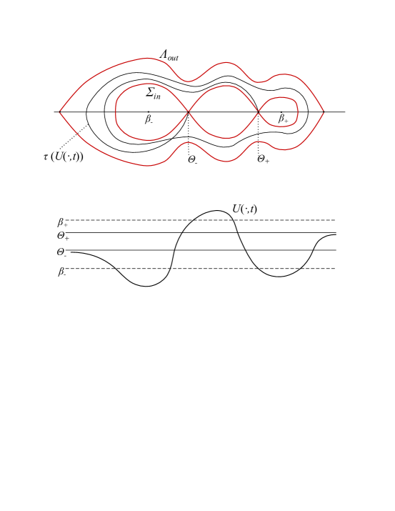
Figure 2: An illustration of relations (4.26) that are ruled out in the proof of Lemma 4.11, in this case $z\left(U(\cdot,t)-\beta_{-}\right)=4$. The top figure depicts the spatial trajectory and the bottom figure the graph of $U(\cdot,t)$. The relation $\Theta_{-}<\Theta_{+}$ chosen for the figure is of no significance; the limits may actually be related the other way or may be equal.

Recall that under condition (C2) the limits $U(\pm\infty,t)=\Theta_{\pm}$ are in $(\beta_{-},\beta_{+})$. By (4.8), $U_{x}(x,t)\neq 0$ whenever $U(x,t)\in[\beta_{-},\beta_{+}].$ It follows that, assuming (4.26), the zero numbers $z(U(\cdot,t)-\Theta_{\pm})$ are finite and greater than or equal to 2, and the zeros being counted are all simple. Moreover, between any two successive zeros of $U(\cdot,t)-\Theta_{-}$ there are (two) zeros of either $U(\cdot,t)-\beta_{-}$ or $U(\cdot,t)-\beta_{+}$. This implies that $z(U(\cdot,t)-\Theta_{-})$ is bounded uniformly in $t$. The same goes for $z(U(\cdot,t)-\Theta_{+})$. Thus, by the monotonicity of the zero number, $z(U(\cdot,t)-\Theta_{\pm})$ are constant in $t$ for all sufficiently large negative $t$, say for all $t<t_{0}$. We define

$$\xi_{-}(t) :=\min\left\{x:U(x,t)=\Theta_{-}\right\}\text{ \ \ (the first zero of $U-\Theta_{-}$)},$$

$$\xi_{+}(t) :=\max\left\{x:U(x,t)=\Theta_{+}\right\}\text{ \ (the last zero of $U-\Theta_{+}$)}.$$

These are well defined and continuous functions of $t$ for $t<t_{0}$. As one checks easily, (4.26) implies that $\xi_{-}(t)<\xi_{+}(t)$. Since $U(\pm\infty,t)=\Theta_{\pm}$, the function $U(\cdot,t)$ is not monotone on $(-\infty,\xi_{-}(t))$, nor it is such on $(\xi_{+}(t),\infty).$ Therefore, by Lemma 2.11, there exists $K>0$ such that

$$-K<\xi_{-}(t)<\xi_{+}(t)<K\quad(t<t_{0}).$$ (4.27)

By (4.8) and (4.26), we have

$$z_{(\xi_{-}(t),\xi_{+}(t))}\left(U(\cdot,t)-\beta_{-}\right)\geq 2\ \,(t<t_{0})\quad\textrm{ or }\quad z_{(\xi_{-}(t),\xi_{+}(t))}\left(U(\cdot,t)-\beta_{+}\right)\geq 2\ \,(t<t_{0}).$$ (4.28)

We consider the latter, the former is analogous. By Theorem 2.10, there is a steady state $\phi$ of (1.1) with $\phi\in\alpha(U)$. Using (4.27), (4.28) and taking into account that between any two successive zeros of $U(\cdot,t)-\beta_{+}$ the function $U(\cdot,t)$ achieves a value greater than $q$ or smaller than $p$, we infer that $\displaystyle z_{(-K,K)}\left(\phi-\beta_{+}\right)\geq 2.$ Obviously, $\tau(\phi)\subset\bar{\Pi}$ and $\phi$ is not a nonconstant periodic solution (see Corollary 4.6). Moreover, because of (4.27), there exist $x_{1},x_{2}$ with $-K\leq x_{1}<x_{2}\leq K$ such that $\phi(x_{1}),\phi(x_{2})\leq\max(\Theta_{-},\Theta_{+}).$ These conditions on $\phi$ leave only one possibility for the steady state $\phi$: $\phi=\Phi(\cdot-x_{0})$ for some $x_{0}\in(-K,K),$ where $\Phi$ is the ground state at level $\gamma=\hat{p}$ as in (A1) (and, necessarily, $\Lambda_{out}$ is a homoclinic loop). We have thus shown that for some sequence $t_{n}\to-\infty,$

$$U(\cdot,t_{n})\underset{n\to\infty}{\longrightarrow}\Phi(\cdot-x_{0})$$

in $L^{\infty}_{loc}(\mathbb{R})$. Notice that from (4.27) it follows that $\Phi(\pm K-x_{0})\leq\max(\Theta_{+},\Theta_{-})<q.$ We show that this leads to a contradiction, which will complete the proof.

Let $\psi$ be any periodic solution of (1.6) with $\tau(\psi)\subset\Pi$ and let $\rho>0$ be the minimal period of $\psi.$ Shifting $\psi$, we may assume that $\psi(K)=\max\psi>q>\Phi(K-x_{0}).$ Then $\Phi(\cdot-x_{0})<\psi$ on $(K,K+\rho)$ (otherwise, a shift of the graph of $\psi$ would be touching the graph of $\Phi(\cdot-x_{0})$, which is impossible for two distinct solutions of (1.6)). Consequently, if $n_{0}$ is large enough, we have $t_{n_{0}}<t_{0}-1$ and

$$U(x,t_{n_{0}})<\psi(x)\quad(x\in(K,K+\rho)).$$

Moreover, since $\xi_{+}(t)<K$ for all $t<t_{0},$ we have

$$U(K,t)<\psi(K)\ \textrm{ and }\ U(K+\rho,t)<\psi(K+\rho)\quad(t<t_{0}).$$

Therefore, applying the comparison principle on $(K,K+\rho)\times(t_{n_{0}},t_{0})$, we obtain

$$U(x,t_{0}-1)<\psi(x)\quad(x\in(K,K+\rho)).$$

This is true for all periodic solutions $\psi$ with the indicated properties. Taking a sequences of such periodic solution with $\psi_{j}(K)\to\Phi(0)$—which entails $\rho\to\infty$ and $\psi_{j}\to\Phi(\cdot-K)$ locally uniformly—we obtain that $U(x,0)<\Phi(x-K),$ $x>K.$ So $U(x,t_{0}-1)\to\gamma$ as $x\to\infty,$ in contradiction to (C2). ∎

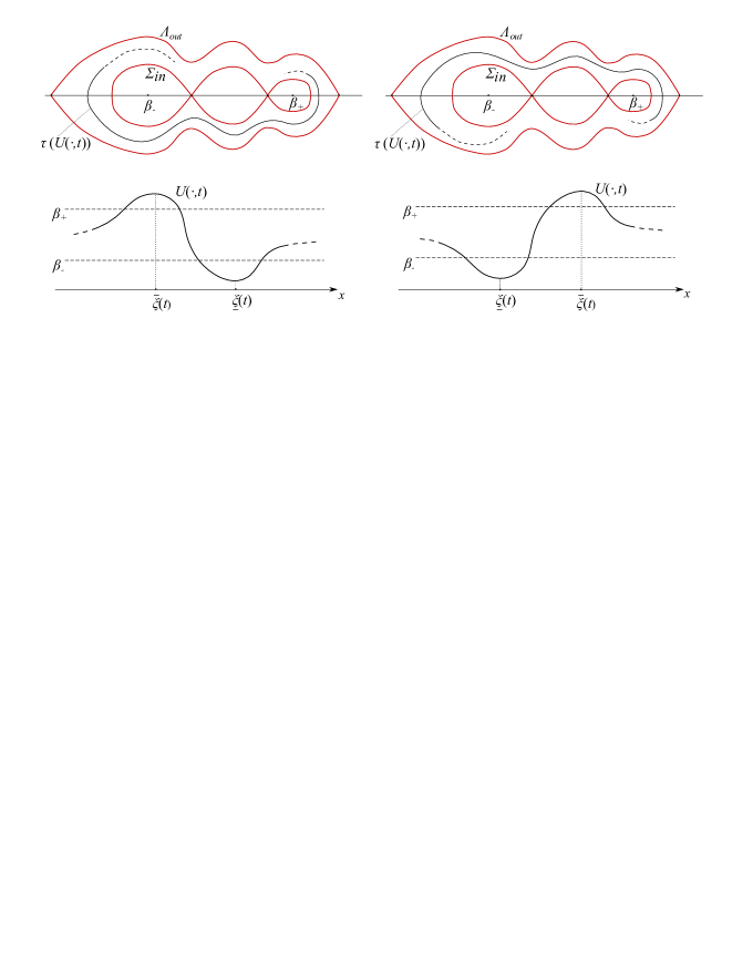
Figure 3: The spatial trajectories and graphs of $U(\cdot,t)$ in the cases $\overline{\xi}(t)<\underline{\xi}(t)$ (the figures on the left) and $\overline{\xi}(t)>\underline{\xi}(t)$ (the figures on the right).

Assuming (4.24), the previous lemma shows that (4.25) holds for all $t\in\mathbb{R}$. Lemma 4.4 now tells us that for every $t$ the function $U(\cdot,t)$ has exactly two critical points $\overline{\xi}(t)$, $\underline{\xi}(t)$, both nondegenerate, which are the global maximum and minimum points of $U(\cdot,t)$, respectively. Since $U(\pm\infty,t)=\Theta_{\pm}\in(\beta_{-},\beta_{+})$, we have

$$U(x,t)>\beta_{-}\ \,(x\in(-\infty,\overline{\xi}(t)),\ t\in\mathbb{R})\quad\textrm{ or }\quad\ U(x,t)>\beta_{-}\ \,(x\in(\overline{\xi}(t),\infty),\ t\in\mathbb{R}),$$ (4.29)

depending on whether $\overline{\xi}(t)<\underline{\xi}(t)$ or $\overline{\xi}(t)>\underline{\xi}(t)$ (cp. Figure 3). Similarly,

$$U(x,t)<\beta_{+}\ \,(x\in(\underline{\xi}(t),\infty),\ t\in\mathbb{R})\quad\textrm{ or }\quad U(x,t)<\beta_{+}\ \,(x\in(-\infty,\underline{\xi}(t)),\ t\in\mathbb{R}).$$ (4.30)

We next prove the conclusion of Proposition 4.1 in the case (C2) when $\Lambda_{out}$ is a homoclinic loop.

Lemma 4.12.

Assume that (C2) and (4.24) hold, $\Lambda_{out}$ is a homoclinic loop as in (A1), and $U$ is not a steady state. Then $\tau(\alpha(U))\subset\Sigma_{in}$ and $\omega(U)=\{\gamma\}$, where $\gamma\in\{\hat{p},\hat{q}\}$ is as in (A1). In particular, (4.4) holds.

Proof.

For definiteness, we assume that $\gamma=\hat{p}$—so $\Phi$ is a ground state at level $\hat{p}$ and $\hat{q}=\Phi(0)$ is its maximum—the case $\gamma=\hat{q}$ is similar. We prove that for some $\vartheta>0$

$$\max_{x\in\mathbb{R}}U(x,t)<\hat{q}-\vartheta\quad(t\in\mathbb{R}).$$ (4.31)

Once this is done, the desired conclusion follows immediately from Lemma 4.8(i).

Assume that (4.31) is not true for any $\vartheta>0$. Then there is a sequence $t_{n}\in\mathbb{R}$ such that $U(\overline{\xi}(t_{n}),t_{n})\nearrow\hat{q}$ (and $U_{x}(\overline{\xi}(t_{n}),t_{n})=0$). As in the proof of Lemma 4.7(i), passing to a subsequence if necessary, we have $U(\cdot+\overline{\xi}(t_{n}),t_{n})\to\Phi$ in $C^{2}_{loc}(\mathbb{R})$. This and the relations $\Phi(\pm\infty)=\gamma=\hat{p}<\beta_{-}$ clearly contradict (4.29). Thus (4.31) indeed holds and the proof is complete. ∎

Figure 4: The graph of $U(\cdot,t)$ when $\overline{\xi}(t)<\underline{\xi}(t)$. The relation $\xi_{+}(t)<\xi_{-}(t)$ holds when $\Theta_{+}>\Theta_{-}$ (as in the figure), it is reversed when $\Theta_{+}<\Theta_{-}$, and $\xi_{+}(t)=\xi_{-}(t)$ when $\Theta_{+}=\Theta_{-}$.

We now treat the case when $\Lambda_{out}$ is a heteroclinic loop.

Lemma 4.13.

Assume that (C2) and (4.24) hold, $\Lambda_{out}$ is a heteroclinic loop as in (A2), and $U$ is not a steady state. Then (4.4) holds: $\tau(\alpha(U))\subset\Sigma_{in}$, $\tau(\omega(U))\subset\Lambda_{out}$.

Proof.

With $\overline{\xi}(t)$, $\underline{\xi}(t)$ as above, we only consider the case $\overline{\xi}(t)<\underline{\xi}(t)$; the arguments in the case $\overline{\xi}(t)>\underline{\xi}(t)$ are similar. Thus (cp. Figure 4)

$$U_{x}(x,t)>0\quad(x\in(-\infty,\overline{\xi}(t))\cup(\underline{\xi}(t),\infty),\ t\in\mathbb{R}),$$ (4.32)

$$U_{x}(x,t)<0\quad(x\in(\overline{\xi}(t),\underline{\xi}(t)),\ t\in\mathbb{R}).$$

As in the proof of Lemma 4.11, we define

$$\xi_{-}(t) :=\min\left\{x:U(x,t)=\Theta_{-}\right\}\text{ \ \ (the first zero of $U-\Theta_{-}$)},$$

$$\xi_{+}(t) :=\max\left\{x:U(x,t)=\Theta_{+}\right\}\text{ \ (the last zero of $U-\Theta_{+}$)}.$$

Clearly, for all $t\in\mathbb{R}$, $\xi_{\pm}(t)$ are defined and

$$\xi_{\pm}(t)\in(\overline{\xi}(t),\underline{\xi}(t))$$ (4.33)

($\xi_{-}(t)$, $\xi_{+}(t)$ may be equal, or ordered either way, depending on the relation between $\Theta_{-}$ and $\Theta_{+}$). Since $\xi_{\pm}(t)$ is a simple zero of $U(\cdot,t)-\Theta_{\pm}$, it is a $C^{1}$ function of $t$.

We split the rest of the proof into several steps.

Step 1. We show that

$$\tau\left(A(U)\right)\subset\Sigma_{in},$$ (4.34)

which in particular gives the first inclusion in Lemma 4.13: $\tau(\alpha(U)\subset\Sigma_{in}$.

It is sufficient to prove that the constants $\gamma_{\pm}$ are not contained in $A(U)$. Indeed, if this holds, then $A(U)$ does not contain any shifts of the standing waves $\Phi_{\pm}$ either (by compactness and translation invariance of $A(U)$). Consequently, by Lemma 4.7, $\displaystyle dist\left(\tau\left(A(U)\right),\Lambda_{out}\right)>0,$ and (4.34) follows upon an application of Lemma 2.13.

Assume, for a contradiction that $\gamma_{+}\in A(U)$ (arguments to rule out the possibility $\gamma_{-}\in A(U)$ are similar and are omitted). Clearly, since $\Theta_{\pm}=U(\pm\infty,t)$, the function $U(\cdot,t)$ is monotone neither on $(-\infty,\xi_{-}(t))$ nor on $(\xi_{+}(t),\infty).$ Therefore, by Lemma 2.11, $\xi_{-}(t)$ is bounded from below and $\xi_{+}(t)$ from above as $t\to-\infty:$ there is a constant $K>0$ such that

$$\xi_{-}(t)>-K,\ \xi_{+}(t)<K,\quad(t<0).$$ (4.35)

Since $\gamma^{+}\in A(U)$, there is a sequence $t_{n}\to-\infty$ such that, denoting $x_{n}:=\overline{\xi}(t_{n})$, we have $U(x_{n},t_{n})\to\gamma_{+}$ (and $U_{x}(x_{n},t_{n})=0$). As in Lemma 4.7(i), passing to a subsequence if necessary, we obtain that the sequence of functions $U_{n}:=U(\cdot+x_{n},\cdot+t_{n})$ converges in $C^{1}_{loc}(\mathbb{R}^{2})$ to $\gamma^{+}$. Moreover, because of (4.33), (4.35), we have $U(K,t)<\Theta_{+}$ for all $t<0,$ thus $x_{n}\to-\infty$ as $n\to\infty.$

Let $\psi$ be any periodic solution of (1.6) with $\tau(\psi)\subset\Pi$ and $\psi(0)>\beta_{+}$, $\psi^{\prime}(0)=0$. Let $2\rho>0$ be the minimal period of $\psi$, so $\psi(0)$ is the maximum of $\psi$, and $\psi(-\rho)=\psi(\rho)<\beta_{-}$ is the minimum of $\psi$. Obviously, for all large enough $n$, say for all $n>n_{0}$, we have

$$U(\cdot+x_{n},t_{n})>\psi\text{ on $[-\rho,\rho]$}.$$

Also, due to (4.35) and the convergence $x_{n}\to-\infty$, we have, making $n_{0}$ larger if necessary,

$$U(\pm\rho+x_{n},t)>\Theta_{-}>\psi(-\rho)=\psi(\rho)\quad(n>n_{0},\ t\in(t_{n},0]).$$

Therefore, by the comparison principle, for $n>n_{0}$,

$$U(x+x_{n},t)>\psi(x)\quad(x\in[-\rho,\rho],\quad t>t_{n}).$$

In particular, at $t=0$, we obtain

$$\max_{x\in[-\rho,\rho]}U(x+x_{n},0)\geq\max\psi>\beta_{+}\quad(n>n_{0}).$$

Since $x_{n}\to-\infty$, we obtain a contradiction to the fact that $U(-\infty,0)=\Theta_{-}<\beta_{+}$. This contradiction completes the proof of (4.34).

Step 2. We show that

$$\tau\left(\omega(U)\right)\subset\Sigma_{in}\textrm{ or }\tau\left(\omega(U)\right)\subset\Lambda_{out}.$$ (4.36)

Note that due to (4.32), in both cases $\Theta_{-}=\Theta_{+}$ and $\Theta_{-}\neq\Theta_{+},$ the solution $U(\cdot,t)$ satisfies the hypotheses of Theorem 2.12. So $\omega(U)$ consists of steady states, and it does not contain non-constant periodic functions (cp. Corollary 4.6). So $\tau(\omega(U))\subset\bar{\Pi}\setminus\mathcal{P}_{0}$ and it is connected. This gives (4.36).

Step 3. In this step we complete the proof of Lemma 4.13 by showing that $\tau(\omega(U))\subset\Lambda_{out}$. In view of (4.36), we just need to rule out the possibility

$$\tau(\omega(U))\subset\Sigma_{in}.$$ (4.37)

Assume it holds. We derive a contradiction. Pick a sufficiently small $\varepsilon>0$ such that

$$\gamma_{-}=\hat{p}<p-\varepsilon,\quad\gamma^{+}=\hat{q}>q+\varepsilon.$$

Relation (4.37) in particular implies that for any $M>0$ there exists $T=T(M)$ such that

$$p-\varepsilon<U(x,t)<q+\varepsilon\quad(x\in(-M,M),\ t>T(M)).$$ (4.38)

By Step 1 and Lemma 4.7(ii), $\Omega(U)$ contains one of the constants $\gamma_{\pm}$ (or a shift of one of the standing waves $\Phi_{\pm}$, and, consequently, also both constants $\gamma_{\pm}$). We only consider the case $\gamma_{+}\in\Omega(U)$, the case $\gamma_{-}\in\Omega(U)$ being similar. Hence, there is a sequence $t_{n}\to\infty$ such that, denoting $x_{n}:=\overline{\xi}(t_{n})$, we have

$$U(\cdot+x_{n},t_{n})\underset{n\to\infty}{\longrightarrow}\gamma_{+},$$ (4.39)

with the convergence in $L^{\infty}_{loc}(\mathbb{R}).$ Clearly, (4.39), (4.38) imply that $|x_{n}|\to\infty$. We claim that necessarily $x_{n}\to-\infty.$ Observe that, by (4.32) and (4.33),

$$U(x,t)>\min(\Theta_{-},\Theta_{+})\quad(-\infty<x<\max\{\xi_{-}(t),\xi_{+}(t\}),$$ (4.40)

$$U(x,t)<\max(\Theta_{-},\Theta_{+})\quad(\min\{\xi_{-}(t),\xi_{+}(t)\}<x<\infty);$$ (4.41)

and $U_{x}(\xi_{\pm}(t),t)<0.$ Using the last relation and Lemma 2.11, we obtain the following monotonicity relations for all $t>0$:

$$\textrm{if }\xi_{-}(t)>\xi_{-}(0), \textrm{ then }U_{x}(\cdot,t)<0\textrm{ on }\left(\xi_{-}(0),\xi_{-}(t)\right),$$ (4.42)

$$\textrm{if }\xi_{+}(t)<\xi_{+}(0), \textrm{ then }U_{x}(\cdot,t)<0\textrm{ on }\left(\xi_{+}(t),\xi_{-}(0)\right).$$ (4.43)

From (4.41) and (4.39), it follows that there is $n_{1}$ such that $\xi_{\pm}(t_{n})>x_{n}$ for all $n>n_{1}$. If for some $n>n_{1}$ it is also true that $x_{n}>\xi_{-}(0)$, then the relations $\xi_{-}(0)<x_{n}<\xi_{-}(t_{n})$ and (4.42) give $U(\xi_{-}(0),t_{n})>U(x_{n},t_{n})$. This inequality can hold only for finitely many $n$, due to (4.38), (4.39). Thus for all large enough $n$ we have $x_{n}\leq\xi_{-}(0)$, hence, since $|x_{n}|\to\infty$, it must be true that $x_{n}\to-\infty$, as claimed.

Pick now a periodic solution $\psi$ of (1.6) with $\tau(\psi)\subset\Pi$ such that $\min\psi<p-\varepsilon$ and $\max\psi>q+\varepsilon$. We shift $\psi$ such that $\max\psi=\psi(0)$. Let $2\rho>0$ be the minimal period of $\psi$. Thus we have

$$\min\psi=\psi(\pm\rho)<p-\varepsilon,\qquad\max\psi=\psi(0)>q+\varepsilon.$$

By (4.39), for $n$ large enough,

$$U(x_{n}+x,t_{n})>\psi(0)=q+\varepsilon\quad(x\in(-\rho,\rho)).$$ (4.44)

By (4.41), necessarily $\xi_{\pm}(t_{n})>x_{n}+\rho$. We now show that for some large enough $n_{0}$, the following must hold in addition to (4.44):

$$U(x_{n_{0}}\pm\rho,t)>\psi(\pm\rho)\quad(t>t_{n_{0}}).$$ (4.45)

If this does not hold, then there exist arbitrarily large $n$ such that for some $\tilde{t}_{n}>t_{n}$ one has $\displaystyle U\left(x_{n}+\bar{\rho},\tilde{t}_{n}\right)=\psi(\bar{\rho})=p-\varepsilon$, where $\bar{\rho}$ is either $-\rho$ or $\rho$. Since $U(\cdot,t)>\min(\Theta_{-},\Theta_{+})$ on $(-\infty,\xi_{+}(t))$ (cp. (4.40)), it follows that $\displaystyle\xi_{+}\left(\tilde{t}_{n}\right)<x_{n}+\bar{\rho}$. But, due to $x_{n}\to-\infty$, we also have $x_{n}+\bar{\rho}<\xi_{+}(0)$ if $n$ is large enough; so, by (4.43), $\displaystyle U\left(\xi_{+}(0),\tilde{t}_{n}\right)<U\left(x_{n}+\bar{\rho},\tilde{t}_{n}\right)=p-\varepsilon$. This cannot be true for arbitrarily large $n$, due to (4.38), so (4.45) must indeed hold for some, arbitrarily large, $n_{0}$.

Using (4.44), (4.45), and the comparison principle, we obtain $U(x_{n_{0}},t)>\psi(0)=q+\varepsilon,$ for all $t>t_{n_{0}}.$ This is a contradiction to (4.38).

We have shown that the assumption (4.37) leads to a contradiction, which concludes the proof of Lemma 4.13. ∎

4.2.3 Case (C3): $(\Theta_{-},0)\in\Sigma_{in}$ and $(\Theta_{+},0)\in\Lambda_{out}$

Our assumption in this subsection is that $(\Theta_{-},0)\in\Sigma_{in}$ and $(\Theta_{+},0)\in\Lambda_{out}$. The case $(\Theta_{+},0)\in\Sigma_{in}$ and $(\Theta_{-},0)\in\Lambda_{out}$ is analogous and will be skipped.

For definiteness, we also assume that $\Theta_{+}=\hat{p}$ (hence $f(\hat{p})=0$); the other possibility, $\Theta_{+}=\hat{q}$, can be treated in an analogous way.

Lemma 4.14.

Under condition (C3), $\tau\left(\omega(U)\right)\subset\Lambda_{out}$.

Proof.

Theorem 2.12 implies that $U$ is quasiconvergent, hence and $\omega(U)$ contains only non-periodic steady states or constant steady states.

If $\Lambda_{out}$ is a heteroclinic loop, as in (A2), we choose a decreasing continuous function $\tilde{u}_{0}$ such that $\tilde{u}_{0}(-\infty)=\gamma_{+}>\tilde{u}_{0}>\gamma_{-}=\tilde{u}_{0}(\infty)$ and $\tilde{u}_{0}\geq U(\cdot,0)$. By the comparison principle, the corresponding solution $\tilde{u}=u(\cdot,\cdot,\tilde{u}_{0})$ of (1.1) satisfies $\tilde{u}(\cdot,t)>U(\cdot,t)$ for all $t>0$. By [16, Theorem 3.1], the (front-like) solution $\tilde{u}(\cdot,t)$ converges in $L^{\infty}(\mathbb{R})$ to a shift of the decreasing standing wave $\Phi^{-}$, say $\Phi^{-}(\cdot-\eta)$, as $t\to\infty$. This implies that for all $\varphi\in\omega(U)$, we have $\varphi\leq\Phi^{-}(\cdot-\eta)$. Now, every $\varphi\in\omega(U)$ is a steady state with $\tau(\varphi)\subset\bar{\Pi}$. Therefore, $\varphi\leq\Phi^{-}(\cdot-\eta)$ implies that $\varphi$ is identical to $\hat{q}=\gamma^{-}$ or to a shift of $\Phi^{-}$. In particular, $\tau(\varphi)\subset\Lambda_{out}$.

If $\Lambda_{out}$ is a homoclinic loop, as in (A1), we have $\gamma=\hat{p}$ since we are assuming that $\Theta^{+}=\hat{p}$ and $f(\hat{p})=0$. The arguments here are similar as for the heteroclinic loop, but instead of a front-like solution, we compare $U$ to a solution which converges to a shift of the ground sate $\Phi$. For that, we find a continuous function $\tilde{u}_{0}$ with the following properties:

• $\tilde{u}_{0}$ is even and monotone nondecreasing in $(-\infty,0)$;

• $\tilde{u}_{0}>\gamma,\quad\tilde{u}_{0}(\pm\infty)=\gamma$;

• $\tilde{u}_{0}(x)\geq U(x,0)$ for all sufficiently large $x>0$;

• the solution $\tilde{u}(\cdot,t):=u(\cdot,t,\tilde{u}_{0})$ converges in $L^{\infty}(\mathbb{R})$ to $\Phi$ as $t\to\infty$.

Such a function $\tilde{u}_{0}$ is provided by [23, Theorem 2.6]. More specifically, take first a continuous function $u_{1}$ satisfying (s1)–(s3) and such that $u_{1}\equiv\beta_{+}$ on the interval $(-\ell,\ell)$ (so, in particular, $u_{1}\leq\beta_{+}$). According to Theorem 2.6 of [23], if $\ell$ is sufficiently large, then for some $\lambda>1/2$ the function $\tilde{u}_{0}:=\gamma+2\lambda(u_{1}-\gamma)$ satisfies (s4) (the corresponding solution $\tilde{u}(\cdot,t)$ is a threshold solution in the terminology of [23]); it obviously satisfies (s1)–(s3) as well.

Since $U(x,0)$ is decreasing for large $x>0$, relations (s1)–(s3) imply that for a sufficiently large $\eta>0$ we have $z(\tilde{u}_{0}(\cdot-\eta)-U(\cdot,0))=1$. Therefore, $z(\tilde{u}(\cdot-\eta,t)-U(\cdot,t))\leq 1$ for all $t>0$. As a consequence, taking into account that the difference of any two steady states (1.1) has only simple zeros, we have $z(\Phi(\cdot-\eta)-\varphi)\leq 1$ for all $\varphi\in\omega(U)$. Therefore, any $\varphi\in\omega(U)$ is identical to $\hat{q}=\gamma$ or to a shift of $\Phi$. In particular, $\tau(\varphi)\subset\Lambda_{out}$.

∎

Turning our attention to $\alpha(U)$, we start with a preliminary lemma.

Lemma 4.15.

Assume (C3) holds. Then $\alpha(U)$ does not contain any function $\varphi$ with $\tau(\varphi)\subset\Lambda_{out}$.

Proof.

We assume that

$$N^{\pm}=z(U(\cdot,t)-\beta_{\pm})>0,$$ (4.46)

the case when $N^{-}=0$ or $N^{+}=0$ having been settled by Lemma 4.8(iii).

Recall that we are also assuming, without loss of generality, that $f(\hat{p})=0$ and $\Theta_{+}=\hat{p}$. Thus, $U(-\infty,t)=\Theta_{-}\in(\beta_{-},\beta_{+})$ and $U(\infty,t)=\hat{p}$ for all $t\in\mathbb{R}.$ Using Lemma 4.4, we obtain that the function $U(\cdot,t)$ is decreasing to $\hat{p}$ as $x\to\infty$, and monotone near $x=-\infty$, and the function $U(\cdot,t)-\Theta_{-}$ has only finitely many zeros, all of them simple, with $N:=z(U(\cdot,t)-\Theta_{-})$ independent of $t$.

We denote by $\eta(t)$ the first zero of $U(\cdot,t)-\Theta_{-}.$ Since $\Theta_{-}=U(-\infty,t)$, the function $U(\cdot,t)$ is not monotone on $(-\infty,\eta(t))$. Therefore, by Lemma 2.11, there is $\kappa\in\mathbb{R}$ such that

$$\eta(t)>\kappa\quad(t<0).$$ (4.47)

We distinguish the following two possibilities

• $U(\cdot,t)<\Theta_{-}$ on $(-\infty,\eta(t))$  ($t\in\mathbb{R}$)

• $U(\cdot,t)>\Theta_{-}$ on $(-\infty,\eta(t))$  ($t\in\mathbb{R}$)

Assume (pi). Then (4.47) implies that for all $t<0$

$$U(x,t)\leq\Theta_{-}<\beta_{+}\quad(x\leq\kappa)$$ (4.48)

and any function in $\alpha(U)$ has to satisfy this relation. In particular, the constant $\hat{q}$ and any shift of $\Phi_{-}$ (if $\Lambda_{out}$ is a heteroclinic loop) are ruled out from $\alpha(U)$. It remains to rule out the constant $\hat{p}$, any shift of the ground state $\Phi$ (if $\Lambda_{out}$ is a homoclinic loop), and any shift of $\Phi_{+}$ (if $\Lambda_{out}$ is a heteroclinic loop). Take any of these functions, denoting it by $\varphi$, and assume for a contradiction that $\varphi\in\alpha(U)$. By (4.48),

$$\varphi(x)\leq\Theta_{-}<\beta_{+}\quad(x\leq\kappa).$$ (4.49)

Take any periodic solution $\psi$ of (1.6) with $\tau(\psi)\subset\Pi$, $\psi(\kappa)=\beta_{+},$ and $\psi^{\prime}(\kappa)>0$. Obviously, there is $\rho>0$ such that $\psi(\kappa-\rho)=\beta_{+}.$ We claim that

$$U(x,t)<\psi\quad(x\in[\kappa-\rho,\kappa],\ t\leq 0).$$ (4.50)

Due (4.48), this follows from the comparison principle if we can find a sequence $t_{n}\to-\infty$ such that the claim is valid for $t=t_{n}$, $n=1,2,\dots$. Note that the function $\varphi$, fixed as above, satisfies $\varphi<\psi$ on $(\kappa-\rho,\kappa)$. This is trivial if $\varphi\equiv\hat{p}$; if $\varphi$ is a shift of the ground state or the increasing standing wave, it follows from (4.49) (otherwise, a shift of the graph of $\psi$ we would be touching the graph $\varphi$ at some point, which is impossible for two distinct solutions of (1.6)). Since $\varphi\in\alpha(U)$, there is a sequence $t_{n}\to-\infty$ such that $U(\cdot,t_{n})\to\varphi$ locally uniformly. This sequence, possibly after omitting a finite number of terms, has the desired property.

Thus, (4.50) has to hold for any periodic solution $\psi$ with the indicated properties. We now choose a sequence of such periodic orbits $\psi_{k}$ converging locally uniformly on $\mathbb{R}$ to a shift of the ground state (if $\Lambda_{out}$ is a homoclinic loop) or a shift of $\Phi_{+}$ (if $\Lambda_{out}$ is a heteroclinic loop). In either case, the relations (4.50) with $\psi=\psi_{k}$, $k=1,2,\dots$ and $t=0$, contradict the relations $U(-\infty,0)=\Theta_{-}>\hat{p}$. This contradiction completes the proof if (pi) holds.

Now assume (pii). Then (4.47) implies that for all $t<0$

$$U(x,t)\geq\Theta_{-}>\hat{p}\quad(x\leq\kappa).$$

Therefore, each function in $\alpha(U)$ has to satisfy this inequality, which shows that the following functions cannot be elements of $\alpha(U)$: the constant $\hat{p}$, any shift of the ground state $\Phi$ (if $\Lambda_{out}$ is a homoclinic loop), any shift of the increasing standing wave $\Phi_{+}$ (if $\Lambda_{out}$ is a heteroclinic loop). Thus, we only need to show that if $\Lambda_{out}$ is a heteroclinic loop, then $\alpha(U)$ does not contain the constant $\hat{q}$ or any shift of $\Phi_{-}$. The arguments for this are analogous to the arguments used in the case (pi) to show that $\alpha(U)$ does not contain the constant $\hat{p}$ or any shift of $\Phi_{+}$ and are omitted. ∎

We conclude this section by the following lemma, which, in conjunction with Lemma 4.14, shows that (4.4) holds in the case (C3) as well.

Lemma 4.16.

Assume (C3). Then $\tau\left(\alpha(U)\right)\subset\Sigma_{in}.$

Proof.

From lemma 4.15 (combined with Lemma 2.9), we know that for any $\varphi_{0}\in\alpha(U),$ the trajectory $\tau(\varphi_{0})$ is disjoint from $\Lambda_{out}.$

Fix an arbitrary $\varphi_{0}\in\alpha(U)$, we need to prove that $\tau(\varphi_{0})\subset\Sigma_{in}$. Let $\tilde{U}$ be the entire solution with $\tilde{U}(\cdot,0)=\varphi_{0}$. Then $\tilde{U}$ satisfies (HU) (cp. Corollary 4.6). Therefore, we may apply to $\tilde{U}$ the results concerning the $\omega$-limit set already proved in this subsection and in the previous two subsections. Thus, if $\varphi_{0}$ is not a steady state, then $\tau(\omega(\tilde{U}))\subset\Lambda_{out}$. This would mean—since $\tau(\omega(\tilde{U}))\subset\alpha(U)$ by the invariance and compactness of $\alpha(U)$—that $\alpha(U)$ contains a function $\varphi$ with $\tau(\varphi)\subset\Lambda_{out}$, in contradiction to Lemma 4.15. Therefore, $\varphi_{0}$ has to be a steady state. It is not periodic (cp. Corollary 4.6) and $\tau(\varphi_{0})$ is not contained in $\Lambda_{out}$ by Lemma 4.15. We are left with the desired option $\tau(\varphi_{0})\subset\Sigma_{in}$, completing the proof. ∎

5 Proof of Proposition 3.2 in the case $\Pi=\Pi_{0}$

Proposition 4.1, proved in the previous section, implies that statement (ii) of Proposition 3.2 holds if $\Pi\neq\Pi_{0}$. We now consider the case $\Pi=\Pi_{0}$ (and so $\Sigma_{in}=\{(0,0)\}$), assuming that conditions (U), (NC), (R) hold. We further assume that $\varphi\in\omega(u)$, $U$ is the entire solution of (1.1) with $U(\cdot,0)=\varphi$, and

$$\underset{t\in\mathbb{R}}{\textstyle\bigcup}\tau\left(U(\cdot,t)\right)\subset\Pi_{0}.$$ (5.1)

We prove that

$$\alpha(U)=\{0\},\qquad\tau\left(\omega(U)\right)\subset\Lambda_{out},$$ (5.2)

thereby completing the proof of Proposition 3.2 (note that $\alpha(U)=\{0\}$ is equivalent to $\tau(\alpha(U))=\{(0,0)\}=\Sigma_{in}$).

We use a similar notation as in the previous section:

$$\hat{p} :=\inf\{a\in\mathbb{R}:(a,0)\in\Pi_{0}\}=\inf\{a\in\mathbb{R}:(a,0)\in\Lambda_{out}\},$$ (5.3)

$$\hat{q} :=\sup\{a\in\mathbb{R}:(a,0)\in\Pi_{0}\}=\sup\{a\in\mathbb{R}:(a,0)\in\Lambda_{out}\}.$$

Thus, $\{\hat{p},\hat{q}\}=\{\gamma,\Phi(0)\}$ if (A1) holds; and $\hat{p}=\gamma_{-}$, $\hat{q}=\gamma_{+}$ if (A2) holds, where conditions (A1), (A2) are as in Section 4 (cp. (4.5), (4.6)).

Recall from Lemmas 3.11, 3.12 that $k:=z(U(\cdot,t))$, $\ell:=z(U_{x}(\cdot,t))$ are finite and independent of $t$, all zeros of $U(\cdot,t)$, $U_{x}(\cdot,t)$ are simple for all $t$, and the zeros of $U_{x}(\cdot,t)$ are contained in an interval $(-d,d)$ independent of $t$. Further, $U(\cdot,t)$ has no positive local minima and no negative local maxima. This means that the zeros and critical points of $U(\cdot,t)$ alternate.

Clearly, one of the following possibilities occurs:

$$k=0 \ell\geq 2 \ell=1 k=1 \ell=1 k=2 \ell=0 k=1$$;  ;   and ;   and ;   and . (5.4)

We differentiate with respect to these four possibilities.

If $k=0,$ then (5.2) is a direct consequence of Lemma 4.8(i).

Next we show that $\ell\geq 2$ is impossible. Assume it holds. Then $U(\cdot,t)$ has at least one zero contained between two successive critical points—hence contained in $(-d,d)$—for all $t$. If $U(\pm\infty,t)\leq 0$, then the function $U(\cdot,t)$ assumes its positive global maximum in $(-d,d)$, at one of the local maxima. We claim that $U$ has to stay below $\hat{q}-\vartheta$ for some $\vartheta>0.$ Assume otherwise: then there exist sequences $(x_{n})$ in $(-d,d)$ and $(t_{n})$ in $\mathbb{R}$ such that $(U(x_{n},t_{n}),U_{x}(x_{n},t_{n}))$ converges to $(\hat{q},0)$ as $n\to\infty,$ and by Lemma 4.7(i), up to a subsequence, $U(\cdot+x_{n},\cdot+t_{n})$ converges in $C^{1}_{loc}(\mathbb{R})$ to some steady state $\phi$ as $n\to\infty$ with $\tau(\phi)\subset\Lambda_{out}.$ On the other hand, $U(\cdot+x_{n},t_{n})$ admits two critical points in $(-d,d)$ where it takes opposite signs, which clearly contradicts the convergence to $\phi$. Thus our claim is proved and Lemma 4.8(i) now implies that $\omega(U)=\{\hat{p}\}$. This, however, is also prevented by the existence of a zero in $(-d,d)$ and we have a contradiction. Similarly one shows that the relations $U(\pm\infty,t)\geq 0$ lead to a contradiction. If $U(-\infty,t)>0>U(\infty,t)$ or $U(-\infty,t)<0<U(\infty,t)$, then, by [16, Theorem 3.1], the (front-like) solution $U(\cdot,t)$ converges as $t\to\infty$ to a standing wave of (1.1) in $C_{b}^{1}(\mathbb{R})$. But this implies that $U(\cdot,t)$ has no critical points in $[-d,d]$, and we have a contradiction again.

Now consider the case $\ell=1=k$. We denote by $\xi(t)$, $\eta(t)$ the critical point and the zero of $U(\cdot,t)$, respectively. For definiteness, we assume that $\xi(t)<\eta(t)$ and $U(\cdot,t)>0$ in $(-\infty,\eta(t))$; the other possibilities that can occur in the case $\ell=k=1$ can be treated similarly. It follows that $\xi(t)$ is the point of positive maximum of $U(\cdot,t).$ First, we dispose of the possibility that $\Lambda_{out}$ is a homoclinic loop. Since $\xi(t)<\eta(t)$ and $\xi(t)$ is the unique critical point of $U(\cdot,t)$, we have $U_{x}(\cdot,t)<0$ in $[\eta(t),\infty)$, in particular $U(\infty,t)<U(\eta(t),t)=0$. Therefore, $U(\infty,t)$ converges to a stable equilibrium of the equation $\dot{\zeta}=f(\zeta)$ as $t\to\infty$. In view (5.1), this equilibrium has to equal $\hat{p}$, which gives $f(\hat{p})=0$. So if $\Lambda_{out}$ is a homoclinic loop as in (A1), the ground state $\Phi$ satisfies $\Phi(\pm\infty)=\hat{p}$ and $\Phi(0)=\hat{q}$. Using Lemma 4.7(i) and the facts that $\Phi$ has two zeros while $U(\cdot,t)$ has only one and that $U(\xi(t),t)>0$ with $\xi(t)$ bounded, one shows easily that the global maximum of $U(\cdot,t)$, namely $U(\xi(t),t)$, has to stay below $\hat{q}-\vartheta$ for some $\vartheta>0$. By Lemma 4.8(i), $\omega(U)=\{\hat{p}\}$, which contradicts the relation $U(\xi(t),t)>0$. We may thus proceed assuming that $\Lambda_{out}$ is a heteroclinic loop, in particular $\hat{p}$, $\hat{q}$ are zeros of $f$. As above, if $U(\xi(t),t)$ stays below $\hat{q}-\vartheta$ for some $\vartheta>0$, then Lemma 4.8(i) yields a contradiction. Thus, there is a sequence $t_{n}\in\mathbb{R}$ such that that $U(\xi(t_{n}),t_{n})\to\hat{q}$ and, then, by Lemma 4.7(i) and the fact that $\xi(t_{n})\in(-d,d)$, up to some subsequence, $U(\cdot,t_{n})\to\hat{q}$ in $L^{\infty}_{loc}(\mathbb{R})$. Obviously, the sequence $\{t_{n}\}$ is unbounded. Pick any periodic solution $\psi$ of (1.6) with $\tau(\psi)\subset\Pi_{0}$ and $\min\psi=\psi(-d)\leq 0$. Let $2\rho>0$ be the minimal period of $\psi$. Then, for any large enough $n$ we have $U(\cdot,t_{n})>\psi$ in $[-d-2\rho,-d]$. Since also $U(\cdot,t)>0\geq\psi(-d)=\psi(-d-2\rho)$ in $(-\infty,-d]$, the comparison principle gives $U(\cdot,t)>\psi$ in $[-d-2\rho,-d]$ for all $t>t_{n}$. Consequently,

$$U(x,t)>\psi(-d-\rho)=\max\psi\quad(x\in[-d-\rho,-d],\,t>t_{n}),$$ (5.5)

since $U_{x}(\cdot,t)>0$ in $(-\infty,-d)$ (the only critical point of $U(\cdot,t)$ is in $(-d,d)$ and it is the maximum point). Using (5.5) and taking admissible periodic solutions with $\max\psi\to\hat{q}$ (and $\rho\to\infty)$, we obtain two conclusions. First, $U(\cdot,t)\to\hat{q}$ in $L^{\infty}_{loc}(-\infty,-d)$ as $t\to\infty$ and, consequently, $\tau(\omega(U))=\{(\hat{q},0)\}\subset\Lambda_{out}$. Second, the sequence $\{t_{n}\}$ has to be bounded from below (otherwise (5.5) leads to $U(\cdot,0)\equiv\hat{q}$, which is absurd). This implies that there is $\vartheta>0$ such that $U(\xi(t),t)<\hat{q}-\vartheta$ for all $t<0$. Lemma 4.8(ii) now shows that $\tau(\alpha(U))=\{(0,0)\}$, completing the proof of (5.2) in the case $\ell=1=k$.

In the case $\ell=1$ and $k=2$, we denote by $\xi(t)$ the unique critical point of $U(\cdot,t)$ and assume for definiteness $U(\xi(t),t)>0$, so $U(\xi(t),t)$ is the global maximum of $U(\cdot,t)$. If $U(\xi(t),t)<0$, the arguments are analogous. Since $k=2$, we have $U(\pm\infty,t)<0$. The possibility $U(\pm\infty,t)=\hat{p}$ can be treated in much the same way as the case (C1) with $\Theta_{-}=\Theta_{+}$ in Subsection 4.2.1: (5.2) holds in this case. Consider the opposite possibility, $U(-\infty,t)>\hat{p}$ or $U(\infty,t)>\hat{p}$. We assume, again just for definiteness, that the former holds. Then, since $U(-\infty,t)$ is a solution of $\dot{\zeta}=f(\zeta)$, $U(-\infty,t)\to 0$ as $t\to-\infty$ and $U(-\infty,t)\to\hat{p}$ as $t\to\infty$. In particular, $f(\hat{p})=0$. If $\Lambda_{out}$ is a heteroclinic loop, it is easy to prove, using [16, Theorem 3.1] as in [30, Proof of Lemma 3.4] for example, that $U(\cdot,t)\to\hat{p}$ as $t\to\infty$, uniformly on $\mathbb{R}$. This, of course, is impossible when $k=2$. Thus $\Lambda_{out}$ has to be a homoclinic loop, as in (A1), and the ground state $\Phi$ satisfies $\Phi(\pm\infty)=\hat{p}$ and $\Phi(0)=\hat{q}$. We claim that there is $\vartheta>0$ such that $U(\xi(t),t)<\hat{q}-\vartheta$ for all $t<0$. Indeed, otherwise, by Lemma 4.7(i) and the boundedness of $\xi(t)$, there is a sequence $t_{n}\to-\infty$ such that $U(\cdot,t_{n})$ approaches a shift of the ground state in $L_{loc}^{\infty}(\mathbb{R})$. This in conjunction with the property that $U(-\infty,t)\to 0$ as $t\to-\infty$ would imply that $U(\cdot,t_{n})$ has more than one critical point if $n$ is large enough, a contradiction to $\ell=1$. Thus, our claim is proved and Lemma 4.8(ii) now implies that $\tau(\alpha(U))=\{(0,0)\}$. For the proof of (5.2), we now prove that $\operatorname{dist}((0,0),\tau(\omega(U)))>0$. Once proved, this will yield a nonstationary periodic orbit ${\mathcal{O}}$ of (2.3) such that $\tau(\omega(U))\subset\mathbb{R}^{2}\setminus{\overline{\mathcal{I}}(\mathcal{O})}$ from which (5.2) follows at once upon an application of Lemma 2.13. Assume for a contradiction that $\operatorname{dist}((0,0),\tau(\omega(U)))=0$. Then Lemma 4.7(i) yields a sequence $(x_{n},t_{n})\in\mathbb{R}^{2}$ such that $t_{n}\to\infty$ and $U(\cdot+x_{n},t_{n})\to 0$ in $C^{2}_{loc}(\mathbb{R})$. This implies that given any periodic solution $\psi$ of (1.6) with $\tau(\psi)\subset\Pi_{0}$ one has $z(U(\cdot,t_{n})-\psi)\to\infty$ as $n\to\infty$. On the other hand, since $U(\pm\infty,0)<0$, picking $\psi$ near 0, so that $\psi>U(\pm\infty,0)$, we obtain that for $t\geq 0$ the zero number $z(U(\cdot,t)-\psi)$ is finite and therefore bounded as $t$ increases to infinity. This contradiction completes the proof of (5.2) in the case $\ell=1$ and $k=2$.

Finally, we deal with the case $\ell=0$ and $k=1$. Clearly, $U(\pm\infty,t)$ are nonzero and have opposite signs. Assume for definiteness that $U(-\infty,t)<0<U(\infty,t)$. The assumption $\ell=0$ then means that $U_{x}>0$ everywhere. Being solutions of $\dot{\zeta}=f(\zeta)$, $U(\pm\infty,t)$ converge to stable equilibria of this equation as $t\to\infty$. By (5.1), these equilibria have to be $\hat{p}$, $\hat{q}$: $U(-\infty,t)\to\hat{p}$, $U(\infty,t)\to\hat{q}$. In particular, $f(\hat{p})=f(\hat{q})=0$ and $\Lambda_{out}$ is a heteroclinic loop. Using [16, Theorem 3.1], we obtain that the (front-like) solution $U(\cdot,t)$ approaches a shift of the increasing standing wave $\Phi_{+}$, as $t\to\infty$, uniformly on $\mathbb{R}$, so $\tau(\omega(U))\subset\Lambda_{out}$. We now claim that $\alpha(U)=\{0\}$. If $U(-\infty,t)=\hat{p}$, $U(\infty,t)=\hat{q}$, our claim can be proved by essentially the same arguments as those used in the case (C1) with $\Theta_{-}<\Theta_{+}$ in Subsection 4.2.1; see the proof of Lemma 4.10, the relevant part starts with “Case (i) of Lemma 4.9.” If $U(-\infty,t)>\hat{p}$, then $U(-\infty,t)\to 0$ as $t\to-\infty$. This, in conjunction with the relation $U_{x}>0$, implies that $\phi\geq 0$ for any $\phi\in\alpha(U)$. Similarly, if $U(\infty,t)<\hat{q}$, then $\phi\leq 0$ for any $\phi\in\alpha(U)$. Thus, if $U(-\infty,t)>\hat{p}$ and $U(\infty,t)<\hat{q}$, we are done: $\alpha(U)=\{0\}$. It remains to consider the possibility when exactly one of this inequalities holds, say $U(-\infty,t)>\hat{p}$ and $U(\infty,t)=\hat{q}$ (the case $U(-\infty,t)=\hat{p}$ and $U(\infty,t)<\hat{q}$ is analogous). If there is $\phi\in\alpha(U)$, $\phi\not\equiv 0$, then $\alpha(U)$ contains the constant $\hat{q}$. To see this take the solution $\tilde{U}$ of (1.1) with $\tilde{U}(\cdot,0)=\phi$ and $\tilde{U}(\cdot,t)\in\alpha(U)$ for all $t\in\mathbb{R}$. Then, since $\phi\geq 0$, $\phi\not\equiv 0$, we have $\tilde{U}(\cdot,t)\to\hat{q}$ in $L^{\infty}_{loc}(\mathbb{R})$. The compactness of $\alpha(U)$ gives $\hat{q}\in\alpha(U)$, as claimed. This, however, can be proven to be contradictory by the same comparison argument involving the function (4.22) as in the proof of Lemma 4.10. This shows that $\alpha(U)=\{0\}$ and completes the proof of (5.2) in the case $\ell=0$, $k=1$.

6 Morse decompositions and the proofs of the quasiconvergence results

In this section, we prove Theorems 1.1, 1.3, and 1.4, giving also a stronger and more precise version of Theorem 1.3, see Theorem 6.4 below. We prepare the proofs by recalling some results concerning Morse decompositions and chain recurrence.

Throughout this section, we assume that $u_{0}$ is as in (1.8)—specifically, $u_{0}\in\mathcal{V}$ and $u_{0}(-\infty)=u_{0}(+\infty)=0$—and the solution of (1.1), (1.2) is bounded. In what follows, the $\omega$-limit set of this solution, $\omega(u_{0})$, is viewed as a compact subset of $L^{\infty}_{loc}(\mathbb{R})$ equipped with the induced topology (in which it is a compact metric space).

We start by recalling the following result of [13, Lemma 6.2]. Consider a bounded set $Y$ in $C_{b}(\mathbb{R})$ which is positively invariant for (1.1), meaning that $\bar{u}_{0}\in Y$ implies that $u(\cdot,t,\bar{u}_{0})\in Y$ for all $t>0$.

Lemma 6.1.

Let $Y$ be a bounded set in $C_{b}(\mathbb{R})$ which is positively invariant for (1.1). Equip $Y$ with a metric from $L^{\infty}_{loc}(\mathbb{R})$. Given any $T>0$, there is $L=L(T)\in(0,\infty)$ such that for each $t\in(0,T)$ the map $\bar{u}_{0}\mapsto u(\cdot,t,\bar{u}_{0}):Y\to Y$ is Lipschitz continuous with Lipschitz constant $L$.

We now consider the solution flow on $\omega(u_{0})$. For any $t\in\mathbb{R}$, let $G(t):\omega(u_{0})\to\omega(u_{0})$ be defined by $G(t)\varphi=U(\cdot,t)$, where $U(\cdot,t)$ is the entire solution of (1.1) with $U(\cdot,0)=\varphi$. As noted in Section 2.2, this entire solution is well (and uniquely) defined and satisfies $U(\cdot,t)\in\omega(u_{0})$ for all $t\in\mathbb{R}$. We claim that the family $G(t)$, $t\in\mathbb{R}$, defines a flow on $\omega(u_{0})$, that is,

• $G(0)$ is the identity on $\omega(u_{0})$,

• $G(t+s)=G(t)G(s)$  ($s,t\in\mathbb{R})$,

• for each $t_{0}\in\mathbb{R}$, the map $G(t_{0})$ is continuous.

Property (i) is obvious. The group property (ii) follows from the uniqueness of $U$ and the time-translation invariance of (1.1). The continuity of $G(t_{0})$ for $t_{0}>0$ follows from Lemma 6.1 applied to $Y=\omega(u_{0})$. Let now $t_{0}<0$. Properties (i) and (ii) imply that $G(t_{0})$ is the inverse to the continuous map $G(-t_{0})$. Since $\omega(u_{0})$ is compact, the inverse is continuous, too.

Obviously, for any fixed $\varphi$, the map $t\mapsto G(t)\varphi:\mathbb{R}\to\omega(u_{0})$ is continuous. In fact, the map $(\varphi,t)\mapsto G(t)\varphi:\omega(u_{0})\times\mathbb{R}\to\omega(u_{0})$ is (jointly) continuous. This can be proved easily using Lemma 6.1, but the fact that the joint continuity follows from the separate continuity in $t$ and $\varphi$ is a general property of flows (see [22, Section 8A]).

Next we note that the flow $G(t)$, $t\in\mathbb{R}$, on $\omega(u_{0})$ is chain recurrent in the following sense. Let $d$ be a metric on $\omega(u_{0})$ compatible with the topology of $L^{\infty}_{loc}(\mathbb{R})$. For any $\varphi\in\omega(u_{0})$, $\varepsilon>0$, $T>0$, there exist an integer $k\geq 1$, real numbers $t_{1},\cdots,t_{k}\geq T$, and elements $\varphi_{0},\cdots,\varphi_{k}\in\omega(u_{0})$ with $\varphi_{0}=\varphi=\varphi_{k}$ such that

$$d(G(t_{i+1})\varphi_{i},\varphi_{i+1})<\varepsilon\qquad(0\leq i<k).$$

This chain recurrence property of the $\omega$-limit set of solutions with compact orbits is well-known from [9, Sect. II.6.3], where it is proved for flows on compact metric spaces. For semiflows, including those generated by parabolic equations, proofs can be found in [7, Lemma 7.5], [26, Proposition 1.5], [17, Lemma 4.5]. Of course, the continuity result 6.1 is needed here, as the limit set $\omega(u_{0})$ is taken with respect to the topology of $L^{\infty}_{loc}(\mathbb{R})$.

Finally, we recall that a Morse decomposition for $G$ is a system ${\mathcal{M}}_{1},\dots,{\mathcal{M}}_{k}$ of mutually disjoint compact subsets of $\omega(u_{0})$ with the following properties:

• For $j=1,\dots,k$, the set ${\mathcal{M}}_{j}$ is invariant under $G$: $G(t)\varphi\in{\mathcal{M}}_{j}$ for all $\varphi\in{\mathcal{M}}_{j}$ and $t\in\mathbb{R}$.

• If $\varphi\in\omega(u_{0})\setminus\cup_{j=1,\dots,k}{\mathcal{M}}_{j}$ and $U(\cdot,t)=G(t)\varphi$ is the corresponding entire solution, then for some $i,j\in\{1,\dots,k\}$ with $i<j$ one has $\alpha(U)\subset{\mathcal{M}}_{i}$ and $\omega(U)\subset{\mathcal{M}}_{j}$.

(Note that in our definition of $\alpha(U)$, $\omega(U)$, we use the convergence in the topology of $L^{\infty}_{loc}(\mathbb{R})$, and the same topology is used on $\omega(u_{0})$.) The following result of [9, Theorem II.7.A] will be instrumental below. The chain recurrence property of the flow $G$ implies that if ${\mathcal{M}}_{1},\dots,{\mathcal{M}}_{k}$ is a Morse decomposition for $G$, then

$$\omega(u_{0})\subset\bigcup_{j=1,\dots,k}{\mathcal{M}}_{j}.$$ (6.1)

In the proofs of our theorems, we build Morse decompositions for $G$ using chains of (2.3). Consider the system

$$\Sigma_{j},\ j=1,\ldots k,$$ (6.2)

of all chains $\Sigma$ of (2.3) with the property that $\Sigma\cap\tau(\omega(u_{0}))\neq\emptyset$ (as noted in Section 2.2, conditions (ND), (MF) imply that there are only finitely many chains).

Given any two distinct chains $\Sigma$, $\tilde{\Sigma}$, we have, according to Lemma 2.8(ii), that either $\Sigma\subset\mathcal{I}(\tilde{\Sigma})$, or $\tilde{\Sigma}\subset\mathcal{I}(\Sigma)$, or else there are periodic orbits ${\mathcal{O}}_{1}$, ${\mathcal{O}}_{2}$ of (2.3) such that $\overline{{\mathcal{I}}}({\mathcal{O}}_{1})\cap\overline{{\mathcal{I}}}({\mathcal{O}}_{2})=\emptyset$ and $\Sigma\subset\mathcal{I}({\mathcal{O}})$, $\tilde{\Sigma}\subset\mathcal{I}(\tilde{\mathcal{O}})$. For chains $\Sigma$, $\tilde{\Sigma}$ intersecting $\tau(\omega(u_{0}))$, the last possibility is ruled out by Lemma 3.6(i). Thus, relabelling the chains in (1.13) if necessary, we may assume that

$$\Sigma_{j}\subset{\mathcal{I}}(\Sigma_{j+1}),\ j=1,\ldots k-1.$$ (6.3)

We will utilize Morse decompositions with Morse sets of the form

$$\{\varphi\in\omega(u_{0}):\tau(\varphi)\subset\Sigma\},$$ (6.4)

or

$$\{\varphi\in\omega(u_{0}):\tau(\varphi)\subset\overline{{\mathcal{I}}}(\Sigma)\},$$ (6.5)

where $\Sigma$ is one of the chains (1.13). Let us prove first of all that these are compact subsets of $\omega(u_{0})$.

Lemma 6.2.

If $\Sigma$ is any of the chains (1.13), then the sets (6.4), (6.5) are closed subsets of $\omega(u_{0})$.

Proof.

We prove the result for (6.4); the proof for (6.5) is similar and is omitted. Assume that $\varphi_{n}$, $n=1,2,\dots$ belong to the set (6.4) and $\varphi_{n}\to\varphi$ in $\omega(u_{0})$. This means, a priori, that $\varphi_{n}\to\varphi$ in $L^{\infty}_{loc}(\mathbb{R})$, but since $\omega(u_{0})$ is compact in $C^{1}_{loc}(\mathbb{R})$ (cp. Section 2.3), we also have $\varphi_{n}\to\varphi$ in $C^{1}_{loc}(\mathbb{R})$. Pick any $x\in\mathbb{R}$. Then $(\varphi_{n}(x),\varphi_{n}^{\prime}(x))\to(\varphi(x),\varphi^{\prime}(x))$. Since the set $\Sigma$ is obviously closed in $\mathbb{R}^{2}$ and $(\varphi_{n}(x),\varphi_{n}^{\prime}(x))\in\tau(\varphi_{n})\subset\Sigma$, we obtain that $(\varphi(x),\varphi^{\prime}(x))\in\Sigma$. Since $x\in\mathbb{R}$ was arbitrary, we have proved that $\varphi$ belongs to the set (6.4). ∎

We are ready to complete the proofs of our main theorems. In proving the quasiconvergence results, Theorems 1.1 and 1.4, our goal is to show that there is a chain $\Sigma$ of (2.3) such that

$$\tau(\omega(u_{0})\subset\Sigma.$$ (6.6)

This inclusion implies, by Lemma 2.9, that $\omega(u_{0})$ consists of steady states of (1.1), and also gives an additional information that the spatial trajectories of the functions in $\omega(u_{0})$ are all contained in one chain.

Proof of Theorems 1.1, 1.4.

We use the chains in (6.2) to define the following sets

$${\mathcal{M}}_{j}:=\{\varphi\in\omega(u_{0}):\tau(\varphi)\subset\Sigma_{j}\},\quad j=1,\dots,k.$$ (6.7)

They are obviously mutually disjoint—as the chains (6.2) are such, cp. (6.3)—and by Lemma 6.2 they are compact in $\omega(u_{0})$. Since the sets ${\mathcal{M}}_{j}$ consist of steady states (cp. Lemma 2.9), they are invariant for $G$. Take now an arbitrary $\varphi\in\omega(u_{0})\setminus\cup_{j=1,\dots,k}{\mathcal{M}}_{j}$, if there is any such $\varphi$, and let $U(\cdot,t)=G(t)\varphi$ be the corresponding entire solution. By the definition of the sets (6.7) and (6.2), $\tau(\varphi)$ is not contained in any chain. Therefore, Proposition 3.2 tells us that—under the hypotheses of Theorem 1.1 or Theorem 1.4— there are two chains $\Sigma_{in}$, $\Sigma_{out}$ such that $\Sigma_{in}\subset{\mathcal{I}}(\Sigma_{out})$ and

$$\tau\left(\alpha(U)\right)\subset\Sigma_{in},\qquad\tau\left(\omega(U)\right)\subset\Sigma_{out}$$ (6.8)

(for $\Sigma_{out}$, we take the chain containing the loop $\Lambda_{out}$, with $\Lambda_{out}$ as in (3.3)). Since $\alpha(U),\omega(U)\subset\omega(u_{0})$, the inclusions (6.8) imply that $\Sigma_{in}=\Sigma_{\ell}$, $\Sigma_{out}=\Sigma_{j}$ for some $\ell,j\in\{1,\dots,k\}$; and $\Sigma_{in}\subset{\mathcal{I}}(\Sigma_{out})$ implies that $\ell<j$. We have thus proved that ${\mathcal{M}}_{1},\dots,{\mathcal{M}}_{k}$ is a Morse decomposition for the flow $G$. From (6.1) and the connectedness of $\omega(u_{0})$ we now conclude that $k=1$, that is, there is only one chain in (6.2) and (6.6) holds for that chain, as desired. ∎

Remark 6.3.

Hypotheses (R) of Theorem 1.4 is only needed in the proof of Proposition 3.2 in the case that (U) holds and $\Pi=\Pi_{0}$ is the connected component of $\mathcal{P}_{0}$ whose closure contains $(0,0)$ (see Section 5). If this part of Proposition 3.2 could be proved under weaker or no conditions in place of (R), then the above proof would work without change.

We next state and prove a stronger version of Theorem 1.3. Recall from Section 3 that if (U) holds, Proposition 3.2 holds true for any connected component $\Pi$ of $\mathcal{P}_{0}$ distinct from $\Pi_{0}.$ .

Theorem 6.4.

Assume that (U) holds. If $\varphi\in\omega(u_{0})$ is such that $\tau(\varphi)$ is not contained in $\Pi_{0}\cup\{(0,0)\}$, then $\varphi$ is a steady state of (1.1).

Obviously, Theorem 1.3 follows from this result.

Proof of Theorem 6.4.

Let $\Lambda_{0}:=\Lambda_{out}(\Pi_{0})$ be the outer loop associated with $\Pi_{0}$ and let $\Sigma_{0}$ the the chain containing the loop $\Lambda_{0}$. Note that ${\mathcal{I}}(\Lambda_{0})=\Pi_{0}\cup\{(0,0)\}$.

We first consider the possibility that

$$\tau(\omega(u_{0}))\cap\overline{\mathcal{I}}(\Sigma_{0})=\emptyset.$$ (6.9)

This in particular implies that $\Sigma_{j}\cap\overline{\mathcal{I}}(\Sigma_{0})=\emptyset$ for $j=1,\dots,k$. In this situation, one can almost verbatim repeat the previous proof to conclude that $k=1$ and $\omega(u_{0})\subset{\mathcal{M}}_{1}$ consists of steady states. We only remark that if $\varphi\in\omega(u_{0})\setminus\cup_{j=1,\dots,k}{\mathcal{M}}_{j}$, then, due to condition (6.9), one has $\tau(\varphi)\cap\Pi_{0}=\emptyset$. Thus Proposition 3.2 applies to $\varphi$.

Now assume that

$$\tau(\omega(u_{0}))\cap\overline{\mathcal{I}}(\Sigma_{0})\neq\emptyset.$$ (6.10)

We distinguish the following two possibilities:

$$\tau(\omega(u_{0})) \not\subset\overline{\mathcal{I}}(\Sigma_{0}),$$ (6.11)

$$\tau(\omega(u_{0})) \subset\overline{\mathcal{I}}(\Sigma_{0}).$$ (6.12)

The first one, (6.11), can actually be ruled out. Indeed, if (6.11) holds, Proposition 3.2 ensures that at least one of the chains (6.2) is disjoint from $\overline{\mathcal{I}}(\Sigma_{0})$. Denoting by $m$ the number of such chains, we list those chains as

$$\tilde{\Sigma}_{1},\dots,\tilde{\Sigma}_{m}.$$ (6.13)

Here, the labels are chosen such that $\tilde{\Sigma}_{i}\subset{\mathcal{I}}(\tilde{\Sigma}_{i+1})$ for $i=1,\ldots m-1$ (cp. (6.3)).

Consider the following subsets of $\omega(u_{0})$:

$${\mathcal{M}}_{0} :=\{\varphi\in\omega(u_{0}):\tau(\varphi)\subset\overline{\mathcal{I}}(\Sigma_{0})\},$$ (6.14)

$${\mathcal{M}}_{j} :=\{\varphi\in\omega(u_{0}):\tau(\varphi)\subset\tilde{\Sigma}_{j}\}\quad(j=1,\dots,m).$$

All these sets are nonempty by (6.11) and the definition of the sets $\tilde{\Sigma}_{j}$. We claim that these sets constitute a Morse decomposition on $\omega(u_{0})$. Clearly, the sets are mutually disjoint. By Lemma 6.2, they are compact in $\omega(u_{0})$. The sets ${\mathcal{M}}_{j}$, $j=1,\dots,m$, consist of steady states (cp. Lemma 2.9), hence they are invariant for $G$. To prove the invariance of ${\mathcal{M}}_{0}$, take any $\varphi\in\omega(u_{0})$ with $\tau(\varphi)\subset\overline{\mathcal{I}}(\Sigma_{0})$ and let $U(\cdot,t)=G(t)\varphi$ be the corresponding entire solution. If $\tau(\varphi)\cap{\mathcal{I}}(\Sigma_{0})\neq\emptyset$, then, by Lemma 3.3, $\tau(U(\cdot,t))\subset{\mathcal{I}}(\Sigma_{0})$—in particular $U(\cdot,t)\in{\mathcal{M}}_{0}$—for all $t\in\mathbb{R}$. Otherwise, $\tau(\varphi)\subset\Sigma_{0}$ and $\varphi$ is a steady state, so $U(\cdot,t)\in{\mathcal{M}}_{0}$ holds trivially. Thus, the invariance of ${\mathcal{M}}_{0}$ is proved.

Take now an arbitrary $\varphi\in\omega(u_{0})\setminus\cup_{j=1,\dots,k}{\mathcal{M}}_{j}$, if there is any such $\varphi$, and let $U(\cdot,t)=G(t)\varphi$ be the corresponding entire solution. We have $\tau(\varphi)\cap\overline{\mathcal{I}}(\Sigma_{0})=\emptyset$ and $\tau(\varphi)$ is not contained in any chain. Applying Proposition 3.2 (with $\Pi\neq\Pi_{0}$), we obtain similarly as in the proof of Theorems 1.1, 1.4, that there are two chains $\Sigma_{in}$, $\Sigma_{out}$ such that $\Sigma_{in}\subset{\mathcal{I}}(\Sigma_{out})$ and

$$\tau\left(\alpha(U)\right)\subset\Sigma_{in},\qquad\tau\left(\omega(U)\right)\subset\Sigma_{out}.$$ (6.15)

Arguing similarly as in the proof of Theorems 1.1, 1.4, we obtain from (6.15) that ${\mathcal{M}}_{0},\dots,{\mathcal{M}}_{k}$ is a Morse decomposition for the flow $G$, and so (6.1) holds. This time, however, since there are at least two Morse sets in (6.14), from (6.1) we obtain a contradiction to the connectedness of $\omega(u_{0})$.

We have thus ruled (6.11), so (6.12) has to hold. Take now any $\varphi\in\omega(u_{0})$ such that $\tau(\varphi)$ is not contained in $\Pi_{0}\cup\{(0,0)\}={\mathcal{I}}(\Lambda_{0})$. Note that, due to Lemma 3.3, $\tau(\varphi)\cap\Pi_{0}=\emptyset$. We claim that $\tau(\varphi)\subset\Sigma_{0}$, in particular, by Lemma 2.9, $\varphi$ is a steady state of (1.1). Once this claim is proved, the proof of Theorem 6.4 will be complete.

Suppose our claim is not true. Then $\tau(\varphi)\cap{\mathcal{I}}(\Lambda)\neq\emptyset$, where $\Lambda$ is a loop in $\Sigma_{0}$ different from $\Lambda_{0}$. We can therefore find a periodic orbit ${\mathcal{O}}$ of (2.3) such that ${\mathcal{O}}\subset{\mathcal{I}}(\Lambda)$ and $\tau(\varphi)\cap\overline{\mathcal{I}}({\mathcal{O}})\neq\emptyset$. Since $\Lambda\neq\Lambda_{0}$, we have $\{(0,0)\}\not\in{\mathcal{I}}({\mathcal{O}})$. Lemma 3.6 now implies that that $\varphi\not\in\omega(u_{0})$ and we have a contradiction. ∎

References

• [1] S. Angenent. The zero set of a solution of a parabolic equation. J. Reine Angew. Math., 390:79–96, 1988.
• [2] T. Bartsch, P. Poláčik, and P. Quittner. Liouville-type theorems and asymptotic behavior of nodal radial solutions of semilinear heat equations. J. Eur. Math. Soc., 13:219–247, 2011.
• [3] P. Brunovský and B. Fiedler. Connecting orbits in scalar reaction diffusion equations. II. The complete solution. J. Differential Equations, 81:106–135, 1989.
• [4] X. Chen and J.-S. Guo. Existence and uniqueness of entire solutions for a reaction-diffusion equation. J. Differential Equations, 212:62–84, 2005.
• [5] X. Chen, J.-S. Guo, and H. Ninomiya. Entire solutions of reaction-diffusion equations with balanced bistable nonlinearities. Proc. Roy. Soc. Edinburgh Sect. A, 136:1207–1237, 2006.
• [6] X.-Y. Chen. A strong unique continuation theorem for parabolic equations. Math. Ann., 311(4):603–630, 1998.
• [7] X.-Y. Chen and P. Poláčik. Gradient-like structure and Morse decompositions for time-periodic one-dimensional parabolic equations. J. Dynam. Differential Equations, 7(1):73–107, 1995.
• [8] Y.-Y. Chen, J.-S. Guo, H. Ninomiya, and C.-H. Yao. Entire solutions originating from monotone fronts to the Allen-Cahn equation. Phys. D, 378/379:1–19, 2018.
• [9] C. Conley. Isolated invariant sets and the Morse index, volume 38 of CBMS Regional Conference Series in Mathematics. American Mathematical Society, Providence, R.I., 1978.
• [10] Y. Du and H. Matano. Convergence and sharp thresholds for propagation in nonlinear diffusion problems. J. Eur. Math. Soc. (JEMS), 12(2):279–312, 2010.
• [11] Y. Du and P. Poláčik. Locally uniform convergence to an equilibrium for nonlinear parabolic equations on $\mathbb{R}^{N}$. Indiana Univ. Math. J., 64:787–824, 2015.
• [12] E. Feireisl. On the long time behaviour of solutions to nonlinear diffusion equations on $\mathbb{R}^{n}$. NoDEA Nonlinear Differential Equations Appl., 4(1):43–60, 1997.
• [13] E. Feireisl and P. Poláčik. Structure of periodic solutions and asymptotic behavior for time-periodic reaction-diffusion equations on $\mathbb{R}$. Adv. Differential Equations, 5:583–622, 2000.
• [14] B. Fiedler and P. Brunovský. Connections in scalar reaction diffusion equations with Neumann boundary conditions. In Equadiff 6 (Brno, 1985), volume 1192 of Lecture Notes in Math., pages 123–128. Springer, Berlin, 1986.
• [15] B. Fiedler and C. Rocha. Heteroclinic orbits of semilinear parabolic equations. J. Differential Equations, 125:239–281, 1996.
• [16] P. C. Fife and J. B. McLeod. The approach of solutions of nonlinear diffusion equations to travelling front solutions. Arch. Ration. Mech. Anal., 65(4):335–361, 1977.
• [17] J. Földes and P. Poláčik. Convergence to a steady state for asymptotically autonomous semilinear heat equations on $\mathbb{R}^{N}$. J. Differential Equations, 251:1903––1922, 2011.
• [18] T. Gallay and S. Slijepčević. Energy flow in extended gradient partial differential equations. J. Dynam. Differential Equations, 13:757–789, 2001.
• [19] T. Gallay and S. Slijepčević. Distribution of energy and convergence to equilibria in extended dissipative systems. J. Dynam. Differential Equations, 27:653–682, 2015.
• [20] J.-S. Guo and Y. Morita. Entire solutions of reaction-diffusion equations and an application to discrete diffusive equations. Discrete Contin. Dynam. Systems, 12:193–212, 2005.
• [21] F. Hamel and N. Nadirashvili. Entire solutions of the KPP equation. Comm. Pure Appl. Math., 52(10):1255–1276, 1999.
• [22] J. E. Marsden and M. McCracken. The Hopf bifurcation and its applications. Springer-Verlag, New York, 1976. With contributions by P. Chernoff, G. Childs, S. Chow, J. R. Dorroh, J. Guckenheimer, L. Howard, N. Kopell, O. Lanford, J. Mallet-Paret, G. Oster, O. Ruiz, S. Schecter, D. Schmidt and S. Smale, Applied Mathematical Sciences, Vol. 19.
• [23] H. Matano and P. Poláčik. Dynamics of nonnegative solutions of one-dimensional reaction-diffusion equations with localized initial data. Part I: A general quasiconvergence theorem and its consequences. Comm. Partial Differential Equations, 41(5):785–811, 2016.
• [24] H. Matano and P. Poláčik. An entire solution of a bistable parabolic equation on $\mathbb{R}$ with two colliding pulses. J. Funct. Anal., 272:1956–1979, 2017.
• [25] H. Matano and P. Poláčik. Dynamics of nonnegative solutions of one-dimensional reaction-diffusion equations with localized initial data. Part II: The generic case. Comm. Partial Differential Equations, to appear.
• [26] K. Mischaikow, H. Smith, and H. R. Thieme. Asymptotically autonomous semiflows: chain recurrence and Lyapunov functions. Trans. Amer. Math. Soc., 347(5):1669–1685, 1995.
• [27] Y. Morita and H. Ninomiya. Entire solutions with merging fronts to reaction-diffusion equations. J. Dynam. Differential Equations, 18:841–861, 2006.
• [28] Y. Morita and H. Ninomiya. Traveling wave solutions and entire solutions to reaction-diffusion equations. Sugaku Expositions, 23:213–233, 2010.
• [29] A. Pauthier and P. Poláčik. Large-time behavior of solutions of parabolic equations on the real line with convergent initial data. Nonlinearity, 31(9):4423–4441, 2018.
• [30] P. Poláčik. Examples of bounded solutions with nonstationary limit profiles for semilinear heat equations on $\mathbb{R}$. J. Evol. Equ., 15:281–307, 2015.
• [31] P. Poláčik. Spatial trajectories and convergence to traveling fronts for bistable reaction-diffusion equations. In A. Carvalho, B. Ruf, E. Moreira dos Santos, S. Soares, and T. Cazenave, editors, Contributions to nonlinear differential equations and systems, A tribute to Djairo Guedes de Figueiredo on the occasion of his 80th Birthday, Progress in Nonlinear Differential Equations and Their Applications, pages 405–423. Springer, 2015.
• [32] P. Poláčik. Threshold behavior and non-quasiconvergent solutions with localized initial data for bistable reaction-diffusion equations. J. Dynamics Differential Equations, 28:605–625, 2016.
• [33] P. Poláčik. Convergence and quasiconvergence properties of solutions of parabolic equations on the real line: an overview. In Patterns of dynamics, volume 205 of Springer Proc. Math. Stat., pages 172–183. Springer, Cham, 2017.
• [34] P. Poláčik. Entire solutions and a Liouville theorem for a class of parabolic equations on the real line. Proc. Amer. Math. Soc., to appear.
• [35] P. Poláčik. Propagating terraces and the dynamics of front-like solutions of reaction-diffusion equations on $\mathbb{R}$. Mem. Amer. Math. Soc., to appear.
• [36] E. Risler. Global relaxation of bistable solutions for gradient systems in one unbounded spatial dimension. preprint.
• [37] E. Risler. Global behaviour of bistable solutions for gradient systems in one unbounded spatial dimension. preprint.
• [38] A. I. Volpert, V. A. Volpert, and V. A. Volpert. Traveling wave solutions of parabolic systems, volume 140 of Translations of Mathematical Monographs. American Mathematical Society, Providence, RI, 1994. Translated from the Russian manuscript by James F. Heyda.
• [39] M. Wolfrum. A sequence of order relations: encoding heteroclinic connections in scalar parabolic PDE. J. Differential Equations, 183:56–78, 2002.