Spin-dependent two-photon Bragg scattering in the Kapitza-Dirac effect

Abstract

We present the possibility of spin-dependent Kapitza-Dirac scattering based on a two-photon interaction only. The interaction scheme is inspired from a Compton scattering process, for which we explicitly show the mathematical correspondence to the spin-dynamics of an electron diffraction process in a standing light wave. The spin effect has the advantage that it already appears in a Bragg scattering setup with arbitrary low field amplitudes, for which we have estimated the diffraction count rate in a realistic experimental setup at available X-ray free-electron laser facilities.

I Introduction

The spin is an intrinsic angular momentum of every elementary particle . While from the theoretical point of view one would identify the spin as a byproduct of the quantization procedure of relativistic wave functions, one might in a classical picture imagine the spin as a tiny spinning sphere. This view might be intuitive, but should be considered as technically incorrect. Nevertheless, one is associating a magnetic moment with a magnetic dipole to the electron, which in the classical imagination of a charged, spinning sphere would be the ‘handle’ to interact with the electron spin. More formally, intrinsic angular momentum is characterized by “unitary representations of the inhomogeneous Lorentz group”, according to Wigner Wigner (1939); Weinberg (1995). From the historical perspective, it seems that the electron spin was initially rather an implication from the need for a consistent explanation for the atomic structure, as well as from spectroscopic observations Morrison (2007), with a first explicit experimental indication from the Stern-Gerlach experiment Gerlach and Stern (1922a, b, c).

Within the scientific applications of present times, spin-dependent electron interaction appears commonly in photo-emission Kirschner et al. (1981); Maruyama et al. (1991), such that interesting applications like spin- and angle-resolved photoemission spectroscopy (SARPES) Meier et al. (2008); He et al. (2010); Bentmann et al. (2011) is possible, with even recording spin-resolved band structure Kutnyakhov et al. (2015); Elmers et al. (2016); Noguchi et al. (2017); Tang et al. (2012). However, these examples have in common that they are bound state systems, in which the electron is not free from interactions with its environment. For isolated electrons, which propagate freely in space, Wolfgang Pauli has already argued in 1932 that an electron interaction with electro-magnetic fields cannot be sensitive to the electron spin in terms of a concept of classical trajectories Pauli (1932). The reason is that the Stern-Gerlach experiment has been carried out with electrically neutral silver atoms instead of charged electrons. For charged particles, however, the Lorentz force from the magnetic field in the Stern-Gerlach experiment requires a precise knowledge of the electron’s initial position and momentum, which is in conflict with the Heisenberg uncertainty relation. Therefore, a common assumption is that “it is impossible, by means of a Stern-Gerlach experiment, to determine the magnetic moment of a free electron” Mott and Massey (1965) and that “Conventional spin filters, the prototype of which is the Stern-Gerlach magnet, do not work with free electrons.” Kessler (1976). Nevertheless, proposals for a longitudinal setup of the Stern-Gerlach experiment with electrons exist Batelaan et al. (1997); Rutherford and Grobe (1998), for a “minimum-spreading longitudinal configuration” Gallup et al. (2001). Also, random spin-flips can be induced by radio frequency field injection and thermal radiation at an electron in a Penning trap Dehmelt (1988, 1990).

Electron diffraction in standing light waves, as first proposed by Kapitza and Dirac Kapitza and Dirac (1933) (see also Federov and McIver (1980); Gush and Gush (1971); Efremov (1999); Efremov and Fedorov (2000); Smirnova et al. (2004); Li et al. (2004)) could be a way to establish a controlled and explicit spin-dependent interaction of electrons with electro-magnetic fields only. A spin-independent Kapitza-Dirac effect has already been experimentally demonstrated for atoms Gould et al. (1986); Martin et al. (1988) and also electrons in a strong Bucksbaum et al. (1988) and weak Freimund et al. (2001); Freimund and Batelaan (2002) interaction regime. Concerning ‘strong’ and ‘weak’ interaction regimes, we follow a characterization from Batelaan Batelaan (2000, 2007), where the recoil shift $\epsilon$ (corresponding to the spacing of the kinetic energy of the different electron diffraction orders) is compared to the ponderomotive amplitude $V_{0}$ of the standing light wave. The system is in the Bragg regime (weak interaction), if $\epsilon\gg V_{0}$ and in the diffraction regime for $\epsilon\ll V_{0}$ (strong interaction). Spin effects Freimund and Batelaan (2003); Rosenberg (2004); Ahrens et al. (2012, 2013); Bauke et al. (2014a, b); Erhard and Bauke (2015); McGregor et al. (2015); Dellweg et al. (2016) and also spin-dependent diffraction Dellweg and Müller (2017a, b); Ahrens (2017); Ebadati et al. (2018, 2019) (ie. sorting of electrons according to their spin state) has been discussed theoretically for the Kapitza-Dirac effect. While the original proposal from Kapitza and Dirac considers a two-photon momentum transfer, higher order photon scattering is possible Ahrens et al. (2012, 2013); McGregor et al. (2015); Dellweg et al. (2016); Dellweg and Müller (2017a, b); Ebadati et al. (2018); Kozák (2018); Ebadati et al. (2019) but might be suppressed for the case of a weak ponderomotive amplitude of the standing wave light field in the Bragg regime. Therefore, possible implementation difficulties of spin-dependent electron diffraction could arise for the case of a higher number of interacting photons or the necessity to wait for larger fractions of a Rabi cycle of the electron quantum state transition, which could hinder the observation of such higher order photon interactions. A further discussion about spin-dependent electron diffraction scenarios in laser fields is carried out in the outlook section VI at the end of this article. We also point out other theoretical investigations of electron spin dynamics in strong laser fields Panek et al. (2002); Ivanov et al. (2004); Boca and Florescu (2009); Krajewska and Kamiński (2013); Skoromnik et al. (2013); King (2015); Del Sorbo et al. (2017); Seipt et al. (2018); Li et al. (2019); Chen et al. (2019); Wen et al. (2019); Fu et al. (2019) as well as spin-independent electron diffraction scenarios with a controlled phase-space construction Kling et al. (2015, 2016); Debus et al. (2019); Kling et al. (2019); Carmesin et al. (2020).

In this article we discuss spin-dependent Kapitza-Dirac diffraction, featuring a two photon interaction (first feature), which takes place in a Bragg scattering scenario (second feature). In this context, the term “two photon interaction” means that the electron absorbs and emits one photon in a classical view of the interaction. The second feature “Bragg scattering scenario” implies that coherent population transfer between the incoming and diffracted mode allows for the statistical observation of the effect at theoretically arbitrary low field amplitudes. The approach is inspired by a previous work of one of us, which is investigating spin properties in Compton scattering Ahrens and Sun (2017). Accordingly, the effect can be achieved by forming a standing light wave from two counterpropagating laser beams, of which one is linearly polarized and the other is circularly polarized. We then predict the existence of a spin-dependent diffraction effect, if a beam of electrons crosses the standing light wave with a momentum of about $1mc$ along the polarization direction of the linearly polarized laser beam, where $m$ is the electron restmass and $c$ the vacuum speed of light.

The article is organized as follows. In section II, we introduce and explain the parameters of our laser-electron scattering scenario. In section III we define the mathematical framework for the description of the spin-dependent electron diffraction effect and discuss the outcome of an analytic solution in terms of time-dependent perturbation theory. We support these considerations with a relativistic quantum simulation in section IV. After having demonstrated the possibility of this type of two-photon spin-dependent electron diffraction in the Bragg regime, we consider the possibility of an experimental implementation of the effect at the Shanghai High Repetition Rate XFEL and Extreme Light Facility (SHINE) in section V. In the final outlook (section VI) we compare our new spin-dependent interaction scheme with other proposals for spin-dependent electron diffraction in the literature. In the appendix, we discuss the perturbative solution of the electron in the standing light wave (appendix A), a Taylor expansion of the analytic spin-dependent electron scattering formula (appendix B), a perturbative solution for an interacting, quantized electron-photon system, from which a relation to Compton scattering is established (appendix C) and expressions of the spin propagation matrix on the tilted spinor basis, which is used in this article (appendix D).

II Conceptual remarks

As mentioned in the introduction, we want to demonstrate the discussed spin effect with a parameter setup which corresponds to the scenario in reference Ahrens and Sun (2017). Accordingly, we consider electron diffraction at a monochromatic, standing light wave along the $x$-axis

$$A_{\mu}(\boldsymbol{x},t)=\frac{1}{2}\left(a_{\mu}e^{-ik_{l}\cdot x}+a_{\mu}^{*}e^{ik_{l}\cdot x}\phantom{e^{ik^{\prime}_{l}\cdot x}}\right.\\ \left.+a_{\mu}^{\prime}e^{-ik^{\prime}_{l}\cdot x}+a_{\mu}^{\prime*}e^{ik^{\prime}_{l}\cdot x}\right)\,.$$ (1)

In Eq. (1) we have introduced the two momentum four-vectors of the two counterpropagating laser beams

$$k^{\mu}_{l}=(k_{l},\boldsymbol{k}_{l})\,,\qquad k^{\prime\mu}_{l}=(k_{l},-\boldsymbol{k}_{l})\,,$$ (2)

with wave vector $\boldsymbol{k}_{l}=k_{l}\boldsymbol{e}_{x}$, laser wave number $k_{l}$ and the two polarizations $a_{\mu}$ and $a_{\mu}^{\prime}$ of the left and right propagating laser beam. Throughout the paper, except the experimental section V, we set $c=\hbar=1$, in a Gaussian unit system, such that laser frequency $\omega$ equals the laser wave number $k_{l}$. The dot between the four-vectors symbolizes a four-vector contraction $k_{l}\cdot x=k_{l}^{\mu}x_{\mu}$ according to Einstein’s sum convention

$$a_{\mu}b^{\mu}=\sum_{\mu}a_{\mu}b^{\mu}\,,$$ (3)

with space-time metric $g_{\mu\nu}=\textrm{diag}(1,-1,-1,-1)$. Also, we use the symbol $*$ for denoting complex conjugation. The right and left propagating beam is linearly and circularly polarized, respectively and described by the corresponding polarization four-vectors

$$a=(0,0,0,\mathfrak{A})^{\textrm{T}}\,,\quad a^{\prime}=(0,0,\mathfrak{A}^{\prime},i\mathfrak{A}^{\prime})^{\textrm{T}}/\sqrt{2}\,,$$ (4)

where $\mathfrak{A}$ and $\mathfrak{A}^{\prime}$ are the field amplitudes of the lasers’ vector potentials and T denotes transposition. The electron has the initial momentum

$$\tilde{\boldsymbol{p}}_{i}=-\boldsymbol{k}_{l}+m\boldsymbol{e}_{z}$$ (5)

and we consider the two $45^{\circ}$ tilted spin states

$$s^{\searrow}=\begin{pmatrix}\cos 11\pi/8\\ \sin 11\pi/8\end{pmatrix}\,,\qquad s^{\nwarrow}=\begin{pmatrix}\cos 15\pi/8\\ \sin 15\pi/8\end{pmatrix}$$ (6)

as initial electron spin configurations in this work.

In this following paragraph, we want to give a rough explanation of why the parameters (4), (5) and (6) are taken as they are. Though spin-dependent terms may appear in electron-laser interactions, they are usually dominated by a spin-independent term, which can be associated with the ponderomotive potential of the laser beam. Thus, spin-dynamics are usually superimposed by pronounced, spin-independent Rabi oscillations Ahrens (2017) which potentially average out the spin effect. However, it is possible that the dominant contribution from the ponderomotive potential can cancel away, for certain configurations of the electron momentum and the laser polarization Ahrens et al. (2013). It seems that there is a continuum of parameters in parameter space (transverse electron momentum and laser polarizations), for which the spin-preserving terms are suppressed. The discussion about the structure of such a parameter space is beyond the scope of this work, but an investigation which shows a continuous variation of parameters, for which experimentally suitable spin dynamics may appear, is under study Wang and Ahrens . Regarding this article, the related parameters in the follow-up study Ahrens and Sun (2017) of reference Ahrens et al. (2013) were constructed according to systematic reasoning. Since this specific spin effect is investigated with particular care in reference Ahrens and Sun (2017), we prefer to use the parameters in Eqs. (4), (5) and (6) over other possible choices of parameters.

In this context, we would like to point out that reference Ahrens and Sun (2017) discusses spin dynamics in Compton scattering, whereas in this article, the in- and outgoing photon of the scattering process is substituted by two counter-propagating laser beams. This means that we describe the spin-dependent electron quantum dynamics in an external classical field of the counter-propagating laser beam background in terms of the Furry picture Furry (1951); Berestetskii et al. (1982); Fradkin et al. (1991). In the limit of low field amplitudes however, where processes linear in the external field amplitudes are of relevance only, both described scenarios (Compton scattering and electron diffraction) have identical scattering amplitudes. Note, that this association of Compton scattering for electrons in low external fields was already pointed out by Ritus, where the Klein-Nishina formula and also the Breit-Wheeler formula were recovered in the low-field limit of an electron (described by the Dirac equation) in a plane wave field Ritus (1985).

The match of Compton scattering and electron diffraction for low fields can be mathematically justified by showing that the perturbative solution of electron quantum dynamics in an external laser field (see appendix A) can be reformulated into perturbative scattering dynamics of one electron and one photon in the context of an interacting many particle electron-photon quantum system. This solution of the single electron-photon interaction can, in turn, be cast into the form of the Compton scattering formula (explained in appendix C.3). We have sketched this lowest order electron-photon interaction process in context of virtual particle fluctuations during the interaction in Fig. 1. The appearing, four different intermediate particle states, denoted by $\Psi_{a}$, $\Psi_{b}$, $\Psi_{c}$ and $\Psi_{d}$ can be associated with the four diagrams (a), (b), (c) and (d) in Fig. 2, which can be further summed up to give the two, vertex exchanged contributions of the Feynman graphs (e) and (f) of Compton scattering.

Figure 1: Particle fluctuations of an interacting photon and electron. (a) When considering the lowest order interaction of an electron with a photon in a quantized photon electron description, one encounters the four different particle fluctuation configurations (quantum states in Eqs. (59)). In the photonic sector in panel (b) one either has absorption and then emission of the incoming and outgoing photon, or one has first emission and then absorption of the outgoing and incoming photon. In the electronic sector in panel (c) one encounters two quantum trajectories, in which either the electron propagates from its initial to its final state or in which the initial electron is accompanied by a virtual electron-positron pair, which then annihilates with the pair’s anti-particle, with the final electron state remaining. The pairwise combination of the two times two processes in the panels (b) and (c) gives the four combinations in panel (a). One can associate these four quantum paths with Feynman graphs, as illustrated in figure 2. Note however, that in contrast to the graphical conventions in Fig. 2, which correspond to Feynman graphs, the roles of vertices and arrows are interchanged in the graphical representation in this figure: The big black dot corresponds to the free propagation of the quantum state, whereas the arrows indicate a change of the quantum state which is caused by the interaction $H_{\textrm{int}}$. See appendix C for more information.

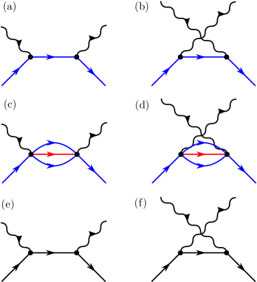
Figure 2: (Color online) Association of Feynman graphs with a corresponding split-up version of the electron-propagator. One can show that the four quantum paths in Fig. 1 with $\Psi_{a}$, $\Psi_{b}$, $\Psi_{c}$ and $\Psi_{d}$ sketched in panels (a), (b), (c) and (d), respectively, can be combined into the Feynman graphs (e) and (f). More precisely, panel (e) is composed of the processes in panels (a) and (c) and panel (f) is composed of the processes in panels (b) and (d). The corresponding mathematical identification is carried out in appendix C.3.

The solutions of time-dependent perturbation theory of a quantized electron-photon system as in Fig. 1 are known as old-fashioned perturbation theory (see literature Halzen and Martin (1984); Weinberg (1995)). Beyond the qualitative picture which is discussed in Figs. 1 and 2, we also give a specific calculation in our article, where both perturbative derivations of the processes can be found in the appendices A and C.

Note, that for the computation of the electron dynamics in the two laser beams, we have chosen the monochromatic standing light wave configuration (1) with laser photon momenta (2), because such an arrangement seems to be more common and is also more suitable for a numerical computation. In general, one could also consider bi-chromatic dynamics or dynamics with non-parallel laser beams. Such a general scenario could however then be related by a Lorentz transformation to our described scenario. In the context of the chosen laser photon momenta (2) and the initial electron momentum (5), a non-trivial interaction with each of the laser beams results in the final electron momentum

$$\tilde{\boldsymbol{p}}_{f}=\boldsymbol{k}_{l}+m\boldsymbol{e}_{z}\,,$$ (7)

as implied by momentum conservation. The longitudinal $x$-component of the initial and final electron momentum is thereby chosen such that also energy is conserved for the electron and photon which constitute to the scattering process in a classical picture.

III Theoretical description

The electron quantum dynamics is computed by making a plane wave decomposition of the electron wave function

$$\psi(\boldsymbol{x},t)=\sum_{n,s}\left(c_{n}^{s}(t)u^{s}_{\boldsymbol{k}_{n}}e^{-i\boldsymbol{k}_{n}\cdot\boldsymbol{x}}+d_{n}^{s}(t)v^{s}_{-\boldsymbol{k}_{n}}e^{-i\boldsymbol{k}_{n}\cdot\boldsymbol{x}}\right)\,.$$ (8)

The approach allows for the transfer of multiple photon momenta $\boldsymbol{k}_{n}=\boldsymbol{p}_{i}+n\boldsymbol{k}_{L}$, with the partial wave’s complex amplitudes $c_{n}^{s}(t)$, $d_{n}^{s}(t)$ for positive and negative solutions, respectively. The positive and negative solutions of the free Dirac equation are the bi-spinors

$$u^{s}_{\boldsymbol{k}} =\sqrt{\frac{m}{\mathcal{E}_{\boldsymbol{k}}}}\sqrt{\frac{\mathcal{E}_{\boldsymbol{k}}+m}{2m}}\begin{pmatrix}\chi^{s}\\ \frac{\boldsymbol{\sigma}\cdot\boldsymbol{k}}{\mathcal{E}_{\boldsymbol{k}}+m}\,\chi^{s}\end{pmatrix}$$ (9a)

$$v^{s}_{\boldsymbol{k}} =\sqrt{\frac{m}{\mathcal{E}_{\boldsymbol{k}}}}\sqrt{\frac{\mathcal{E}_{\boldsymbol{k}}+m}{2m}}\begin{pmatrix}\frac{\boldsymbol{\sigma}\cdot\boldsymbol{k}}{\mathcal{E}_{\boldsymbol{k}}+m}\chi^{s}\\ \chi^{s}\end{pmatrix}\,,$$ (9b)

where $s$ denotes the spin of each wave. The $\boldsymbol{p}_{i}$ is the initial electron momentum, whose transverse component can differ from Eq. (5) at the stage of derivation and $\mathcal{E}_{\boldsymbol{k}}=\sqrt{m^{2}+\boldsymbol{k}^{2}}$ is the relativistic energy momentum relation of the electron. The vector $\boldsymbol{\sigma}$ is the vector $(\sigma_{1},\sigma_{2},\sigma_{3})^{\textrm{T}}$ of the Pauli matrices

$$\sigma_{x}=\begin{pmatrix}0&1\\ 1&0\end{pmatrix}\,,\ \sigma_{y}=\begin{pmatrix}0&-i\\ i&0\end{pmatrix}\,,\ \sigma_{z}=\begin{pmatrix}1&0\\ 0&-1\end{pmatrix}\,,$$ (10)

where we use the indices $\{1,2,3\}$ and $\{x,y,z\}$ interchangeably for indexing Pauli matrices in this article. The dot between 3 component spacial vectors in Eq. (8) is denoting the inner product in Euclidean space $\boldsymbol{k}_{n}\cdot\boldsymbol{x}=\sum_{a}\boldsymbol{k}_{n,a}x_{a}$. The two component objects $\chi^{s}=(\chi_{1}^{s},\chi_{2}^{s})^{\textrm{T}}$ denote spinors. Note that in Refs. Ahrens et al. (2013); Ahrens (2017) the spinors $v^{s}_{\boldsymbol{k}}$ (see Eq. (9b)) have been introduced with opposite momentum $\boldsymbol{k}$. We also point out, that we have absorbed the phase space factor $(m/\mathcal{E}_{\boldsymbol{k}})^{1/2}$ from the Compton cross section formula into the normalization of the spinor definition (9). Furthermore, we mention that the form of the wave function’s plane wave expansion in Eq. (8) is an implication from the standing light wave (1).

The time evolution of the wave function (8) in terms of its expansion coefficients can be formally written as

$$c^{s}_{n}(t) =\sum_{a,s^{\prime}}\left[U_{n,a}^{+,s;+,s^{\prime}}(t,0)c_{a}^{s^{\prime}}(0)+U_{n,a}^{+,s;-,s^{\prime}}(t,0)d_{a}^{s^{\prime}}(0)\right]$$

$$d^{s}_{n}(t) =\sum_{a,s^{\prime}}\left[U_{n,a}^{-,s;+,s^{\prime}}(t,0)c_{a}^{s^{\prime}}(0)+U_{n,a}^{-,s;-,s^{\prime}}(t,0)d_{a}^{s^{\prime}}(0)\right]\,.$$ (11)

A perturbative expression of the propagation functions $U_{n,a}^{\gamma,s;\gamma^{\prime},s^{\prime}}(t,0)$ can be provided by transforming the Dirac equation

$$i\dot{\psi}(\boldsymbol{x},t)=\left[\left(-i\boldsymbol{\nabla}-\textrm{e}\boldsymbol{A}(\boldsymbol{x},t)\right)\cdot\boldsymbol{\alpha}+m\beta\phantom{A^{0}}\right.\\ +\left.\textrm{e}A^{0}(\boldsymbol{x},t)\right]\psi(\boldsymbol{x},t)$$ (12)

into momentum space and applying second order time-dependent perturbation theory to the resulting equations of motion. In Eq. (12), the $\boldsymbol{\alpha}$ and $\beta$ are the Dirac matrices

$$\alpha_{i}=\begin{pmatrix}0&\sigma_{i}\\ \sigma_{i}&0\end{pmatrix}\,,\quad\beta=\begin{pmatrix}\mathds{1}&0\\ 0&\mathds{-1}\end{pmatrix}\,,$$ (13)

where $\mathds{1}$ is the $2\times 2$ identity matrix. The elementary electric charge e simplifies into the square root of the fine structure constant $\textrm{e}=\sqrt{\alpha}$ in our chosen unit system. The dot on top of the wave function $\psi(\boldsymbol{x},t)$ in Eq. (12) denotes its time derivative $\dot{\psi}(\boldsymbol{x},t)=\partial\psi(\boldsymbol{x},t)/\partial t$. The procedure of rewriting and perturbatively solving the Dirac equation in a momentum space description is similar to corresponding procedures in references Ahrens et al. (2013); Bauke et al. (2014b). Therefore, we have shifted the details of the calculation to appendix A and focus on the physics description here.

The perturbative solution of the spin dependent quantum state propagation of the initial electron spin state $c_{0}(0)$ to the final electron spin state $c_{2}(0)$ is proportional to the matrix

$$M_{s}=\frac{1}{\sqrt{8}}\begin{pmatrix}-1&-1-\sqrt{2}\\ -1+\sqrt{2}&1\end{pmatrix}=s^{\nwarrow}\cdot s^{\searrow\dagger}$$ (14)

for our chosen parameters of the photon polarization (4) and the initial electron momentum (5). We take this spin-propagation matrix from the Taylor expansion of the spin propagation matrix $M$ in appendix B. In this context we point out that we desire that spin preserving terms (terms proportional to $\mathds{1}$) cancel in the electron spin dynamics, as mentioned above. This is approximately the case for the transverse momenta of $\tilde{\boldsymbol{p}}_{i}$ in Eq. (5). However, small corrections remain, such that we choose

$$\left(\tilde{\boldsymbol{p}}_{i}\right)_{3}\approx\left(1+1.34...\cdot 10^{-4}\right)m$$ (15)

for the $z$-component of the electron momentum in our numerical simulation with the selected laser photon energy of $k_{l}=13\,\textrm{keV}=0.025...m$. Nevertheless, the corrections to $\tilde{\boldsymbol{p}}_{i}$ are more than two orders of magnitude smaller than the photon momentum $k_{l}$ itself, such that the correction (15) has no strong influence on the physics which is discussed in this work.

The right-hand side of Eq. (14) shows an outer product representation of $M_{s}$, created from the pair of two-component spinors $s^{\nwarrow}$ and $s^{\searrow}$. This can be seen from their expressions

$$s^{\searrow} =\begin{pmatrix}1-\sqrt{2}\\ -1\end{pmatrix}\sqrt{2(2-\sqrt{2})}^{-1}$$ (16a)

$$s^{\nwarrow} =\begin{pmatrix}1+\sqrt{2}\\ -1\end{pmatrix}\sqrt{2(2+\sqrt{2})}^{-1}\,,$$ (16b)

which are equivalent to the definitions (6) and in consistence with the convention in reference Ahrens and Sun (2017). From the outer product representation of the matrix $M_{s}$ at the right-hand side of Eq. (14) one immediately obtains

$$\braket{s^{\searrow}}{M_{s}}{s^{\searrow}} =0 \braket{s^{\nwarrow}}{M_{s}}{s^{\searrow}} =1$$ (17a)

$$\braket{s^{\searrow}}{M_{s}}{s^{\nwarrow}} =0 \braket{s^{\nwarrow}}{M_{s}}{s^{\nwarrow}} =0\,,$$ (17b)

which is consistent with the corresponding scenario in Compton scattering Ahrens and Sun (2017), where a $s^{\searrow}$ polarized electron is scattered at a vertically polarized photon into a left circularly polarized photon and a $s^{\nwarrow}$ polarized electron. The opposite scenario, where a $s^{\nwarrow}$ polarized electron is scattered into a right circularly polarized photon and a $s^{\searrow}$ polarized electron (see reference Ahrens and Sun (2017)) is considered to be overruled by the effect of induced emission into a left circularly polarized photon for the case of coherent electron diffraction with the laser polarization (4) in the Kapitza-Dirac scattering.

IV Numerical solution of the spin-dependent quantum dynamics

We support the above considerations by performing numerical simulations of the one-particle Dirac equation in momentum space (26) (ie. a numerical solution of the propagation equation (11)), of an electron in a standing wave of light in Fig. 3. Such a procedure is similar to the numerical simulations shown in references Ahrens et al. (2012, 2013); Bauke et al. (2014a, b); Erhard and Bauke (2015); Dellweg et al. (2016); Dellweg and Müller (2017b); Ahrens (2017); Ebadati et al. (2018). In the simulation, the standing wave of light (1) has the polarization (4). The standing wave’s field amplitude is smoothly ramped up and down for the duration of five laser periods at the beginning and the end of the simulation by a $\sin^{2}$ temporal envelope, as done in the references Ahrens et al. (2012, 2013); Bauke et al. (2014a, b); Erhard and Bauke (2015); Dellweg et al. (2016); Dellweg and Müller (2017b); Ahrens (2017); Ebadati et al. (2018).

In the numerical simulation, we see no diffraction dynamics for an electron with initial $s^{\nwarrow}$ spin configuration, ie. we have

$$\left|\Braket{s^{\nwarrow}}{U_{0,0}^{+;+}(t,0)}{s^{\nwarrow}}\right|^{2} \approx 1$$ (18a)

$$\left|\Braket{s^{\searrow}}{U_{0,0}^{+;+}(t,0)}{s^{\nwarrow}}\right|^{2} \approx 0$$ (18b)

$$\left|\Braket{s^{\nwarrow}}{U_{2,0}^{+;+}(t,0)}{s^{\nwarrow}}\right|^{2} \approx 0$$ (18c)

$$\left|\Braket{s^{\searrow}}{U_{2,0}^{+;+}(t,0)}{s^{\nwarrow}}\right|^{2} \approx 0\,.$$ (18d)

This is consistent to our analytic considerations from perturbation theory, see Eq. (17b). For this reason we only show the projection on the diffracted spin state

$$\left|\Braket{s^{\nwarrow}}{U_{2,0}^{+;+}(t,0)}{s^{\searrow}}\right|^{2}$$ (19a)

and the initial quantum state

$$\left|\Braket{s^{\searrow}}{U_{0,0}^{+;+}(t,0)}{s^{\searrow}}\right|^{2}$$ (19b)

of the numerical solution of the propagation $U^{+,+}_{a,b}(t,0)$ in Fig. 3. In fact, these are the only non-negligible contributions of the time evolution. Equivalently, one can say that both expressions (19b) sum up to approximately 1, such that the unitarity of the Dirac equation implies that any other excitations are negligibly small.

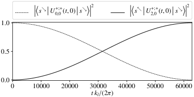
Figure 3: Simulated spin-dependent electron diffraction effect. The panel shows the two non-vanishing matrix elements of the numerical solution of the Dirac equation in momentum space (26), represented by the quantum state propagation (11). The simulation is carried out with the field amplitudes $\mathfrak{A}$ and $\mathfrak{A^{\prime}}$ and laser photon energy $k_{l}$ as specified in Eq. (24), where the initial electron momentum is $\tilde{\boldsymbol{p}}_{i}$ (see Eq. (5)). One can see that the system follows the simple Rabi model (21), from an electron with initial momentum $k_{0}$ and spin state $s^{\searrow}$ into an electron with final momentum $k_{2}$ and spin state $s^{\nwarrow}$. For the opposite initial spin configuration $s^{\nwarrow}$ we find that no such Rabi oscillations occur, which demonstrates a theoretically perfect spin filtering and spin polarization effect.

Note, that the half period Rabi cycle, which is shown in Fig. 3 lasts for $6.29\times 10^{4}$ optical cycles of the laser field, corresponding to the Rabi frequency

$$\Omega_{R}=2.02\times 10^{-7}\,m$$ (20)

in the effective Rabi model

$$\left|\Braket{s^{\nwarrow}}{U_{2,0}^{+;+}(t,0)}{s^{\searrow}}\right|^{2}=\sin\left(\frac{\Omega_{R}t}{2}\right)^{2}\,.$$ (21)

This is consistent with the approximate equation for the matrix element

$$\left|\Braket{s^{\nwarrow}}{U_{2,0}^{+;+}(t,0)}{s^{\searrow}}\right|^{2}\approx\left(\frac{\textrm{e}\mathfrak{A}\textrm{e}\mathfrak{A}^{\prime}k_{l}t}{8m^{2}\sqrt{2}}\right)^{2}$$ (22)

of the perturbative solution of the Dirac equation in Eq. (38). In this context, we assume that the left-hand side of Eq. (22) can be identified with the analytic short time approximation of the Rabi model (21)

$$\left|\Braket{s^{\nwarrow}}{U_{2,0}^{+;+}(t,0)}{s^{\searrow}}\right|^{2}\approx\left(\frac{\Omega_{R}t}{2}\right)^{2}\,,$$ (23)

where we have set the parameters

$$\textrm{e}\mathfrak{A}/m=\textrm{e}\mathfrak{A^{\prime}}/m =4.74\times 10^{-2}$$ (24a)

$$k_{l}/m =2.54\times 10^{-2}$$ (24b)

in our numerical simulation. We choose the photon energy to be 13 keV, corresponding to the value of $k_{l}$ in Eq. (24b) for the simulation. Similarly, we have set the simulation’s laser field amplitude $\mathfrak{A}$ and $\mathfrak{A^{\prime}}$ in (24a), such that a half Rabi period will last exactly 20 fs. This value corresponds to the value of the Rabi frequency (20).

The actual numerical implementation was carried out in the basis of the states $c^{s}_{n}$ and $d^{s}_{n}$ with spin up and spin down $s\in\{\uparrow,\downarrow\}$, where the matrix elements with respect to the spin states $s^{\searrow}$ and $s^{\nwarrow}$ of the numerical propagation $U^{+,+}_{a,b}(t,0)$ are given explicitly in appendix (D). Note that the transition amplitudes $U_{n,0}(t,0)$ of higher momentum states $|n|$ are dropping off exponentially for the chosen parameters in Eq. (24), such that we have truncated the higher modes in the numerical solutions at $|n|=12$, similar to the procedure in references Ahrens et al. (2012, 2013); Bauke et al. (2014a, b); Erhard and Bauke (2015); Dellweg et al. (2016); Dellweg and Müller (2017b); Ahrens (2017); Ebadati et al. (2018).

We want to point out that Eqs. (17) demonstrate a spin-dependent diffraction effect: While the initial spin configuration $s^{\searrow}$ is diffracted into a $s^{\nwarrow}$ configuration, an initial spin $s^{\nwarrow}$ is not diffracted at all! Thus, electrons are filtered according to their initial spin orientation. Also, the outer product in (14) implies that whatever electron spin is diffracted, the final electron spin will always be $s^{\nwarrow}$. This also demonstrates that the electron spin can be polarized by the diffraction mechanism. These two properties (filtering and polarization of the electron spin) are the same characterizations which we have already pointed out in our previous work Ahrens (2017), where a two-photon spin-dependent diffraction is presented which has similar properties as in this work. However, the spin-dependent diffraction effect in reference Ahrens (2017) only appears after multiple Rabi cycles, whereas the spin-dependent diffraction in our current work appears already with the rise of the transition’s oscillation in the form of a Bragg peak, which appears to be more suitable for the experimental implementation.

We also want to point out that the spin-dependent propagation matrix in Eq. (14) is a generalization of our statement in reference Ahrens (2017), in which a spin-dependent quantum state propagation has been identified to be proportional to a projection matrix. In contrast, Eq. (14) demonstrates explicitly that even a projection is not the most general characterization for spin-dependent dynamics. A general and specific criterion for spin-dependent diffraction dynamics might be non-trivial and be a subject of future investigations.

V Experimental implementation considerations

We want to discuss a possible experimental implementation of the spin-dependent laser electron interaction, according to the setup in Fig. 4. In this example, the source of the X-ray laser beams is assumed to be the Shanghai High Repetition Rate XFEL and Extreme Light Facility (SHINE), which is currently under construction Shen et al. (2018). Within its design parameters, SHINE will provide 100 GW laser pules at 13 keV photon energy and with a pulse duration of 20 fs. When the beam is focused to 100 nm, the peak intensity reaches $1.2\times 10^{21}\textrm{W}/\textrm{cm}^{2}$. A coincident laser pulse overlap at the interaction point is achieved by reflecting the two beams as in the arrangement in Fig. 4. Circular polarization can be converted from the linear polarized laser beam by utilizing a phase retardation setup in X-ray diffraction Suzuki et al. (2014). In this way, two coincident, counterpropagating, high intensity pulses can be established at the beam focus, with a linearly polarized beam from the left and a circularly polarized beam from the right. By assuming mirror reflectivities of $85\%$, a phase retarder transmittivity of $55\%$ and a beam splitter design with $34\%$ transmission and $56\%$ reflection Osaka et al. (2013) one estimates an intensity of $1.2\times 10^{20}\,\textrm{W}/\textrm{cm}^{2}$ for the left and right beam at the laser focus spot. Eq. (22) can be written in terms of SI units as

$$\left|\Braket{s^{\nwarrow}}{U_{2,0}^{+;+}(t,0)}{s^{\searrow}}\right|^{2}\approx\left(\frac{\alpha\lambda_{c}^{2}}{8\pi\sqrt{2}}\frac{I_{1}^{1/2}I_{2}^{1/2}t}{c\hbar k_{l}}\right)^{2}\,.$$ (25)

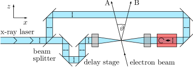
Figure 4: (Color online) Possible experimental setup for establishing spin-dependent electron diffraction based on two photon Kapitza-Dirac scattering. A linearly polarized X-ray laser with 13 keV photon energy is entering from the left. A part of the beam is transmitted through the beam splitter and the reflected part of the X-ray laser beam is guided to approach the beam focus from the opposite direction. A phase retarder (red box with an opened arrow circle) is converting the linear X-ray polarization into circular polarization. All X-ray optics are chosen such that the two counterpropagating laser beams are reaching the beam focus with equal intensity and at equal time. For the setup, spin-dependent diffraction is expected to be observed for initially spin-polarized electrons, which approach the laser focal spot with a kinetic energy of 212 keV at an inclination angle $90^{\circ}-\vartheta/2$ to the beam propagation direction (see main text for details). The small, grey, rectangular boxes are symbolizing beam focussing optics.

Here, $\alpha$ is the fine-structure constant and $\lambda_{c}$ the Compton wavelength and $I_{1}$ and $I_{2}$ are the intensities of the left- and right propagating laser beams. Evaluated with the parameters above, one is expecting a probability of about $1.1\cdot 10^{-7}$ for an electron with a spin $\searrow$ orientation to be diffracted in the direction of beam $B$. Since we are discussing a spin-dependent diffraction scheme, electrons with spin $\nwarrow$ orientation will not be diffracted into beam $B$. For undergoing spin-dependent diffraction, the electrons have to have the specific momentum of $511\,\textrm{keV}/c$ along the $z$-axis, corresponding to a kinetic energy 212 keV. When undergoing diffraction, the electron will pick up two longitudinal photon momenta of $13\,\textrm{keV}/c$ along the $x$-axis. Since the momentum change is longitudinal, one can relate this to a diffraction angle of $\vartheta=2.9^{\circ}$ from the scattering geometry. Spin polarized electron pulses with charges of 10 fC are available Kuwahara et al. (2012) and with the temporal electron bunch width of 10 ps, one expects 124 electrons to cross the beam focal spot in its 20 fs duration. Therefore, with the SHINE aimed repetition rate of 1 MHz we estimate a countrate of 13 electrons per second for the spin-dependent electron diffraction effect. Similar parameters for establishing the considered experimental configuration can also be reached at the LCLS in Stanford lcl ; *Lutman_2018_high_power_xfel and the European X-FEL in Hamburg x-f ; *Altarell:etal:2007:XFEL.

VI Discussion and Outlook

In this article we have discussed a spin-dependent Kapitza-Dirac diffraction effect, which can be implemented in the form of a Bragg scattering setup and which requires only the interaction with two of the standing light wave’s photons. Open questions for the effect are the influence of the laser beam focus on the spin-dependent electron dynamics. Within this article, we have treated the laser beam and also the electron wave function as a discrete superposition of a finite number of plane waves, whereas a Gaussian beam and a Gaussian wave packet would model electron and laser more realistically. In this context the question arises, how a small longitudinal field component Salamin (2006), which is implied by the laser beam focus, is influencing the spin dynamics. Also, the contribution of spontaneous emission of electro-magnetic radiation as compared to the induced emission into the laser beam is of relevance and can be computed Mocken and Keitel (2005). The question on how the quantum state of the laser field is modified by the electron diffraction dynamics is also of relevance, because the Compton scattering version of the effect raises questions about the transfer of intrinsic angular momentum (spin) between the electron and the photon Ahrens and Sun (2017).

There are two possible laser frequency regimes for the implementation of the effect, which are realistic in terms of available laser intensity for the experiment: The optical regime and the x-ray regime.

The optical regime has the advantage that the classical nonlinearity parameter $\xi=\textrm{e}\mathfrak{A}/m$ can reach values of 1 with comparably low effort, such that high photon number Kapitza-Dirac scattering, as for example discussed in references Ahrens et al. (2012, 2013); McGregor et al. (2015); Dellweg et al. (2016); Dellweg and Müller (2017a, b); Ebadati et al. (2018); Kozák (2018); Ebadati et al. (2019) could be possible. Note, that the short-time diffraction probability and the transition’s Rabi frequency are proportional to the field amplitude $\mathfrak{A}$ to the power of the number of interacting photons, implying that either $\xi$ should be close to 1 or the number of contributing photons should be as small as possible. Bi-chromatic setups Dellweg and Müller (2017b); Ebadati et al. (2018) appear promising for the experiment due to potentially long laser-electron interaction times caused by low initial and final electron momenta. However, one challenge with optical systems would be the control of the transverse electron momentum and the laser polarization such that the effect does not smear out. A look on the matrix (41) of the polarization dependent spin dynamics for the electron in the laser beam tells that the electron momentum should be under control on the order of the photon momentum $k_{l}$. Also the laser polarization should be controlled on the accuracy level $k_{l}/m$, where we have $k_{l}\approx 10^{-6}m$ in the optical regime.

In the x-ray regime, on the other hand, this need of fine tuning would be only at the percent level. Here, one faces the challenge of providing field amplitudes, such that $\xi$ is close to one, which might be possible for the case of small beam foci. Therefore, for implementing a spin-dependent diffraction setup for x-rays, a lower order photon interaction Kapitza-Dirac effect would be beneficial. Two photon scattering would be the lowest possible configuration for Kapitza-Dirac-like scattering, since a one-photon interaction is not compatible with the conservation of energy and momentum. A two-photon setup from a previous investigation which only depends on a longitudinal electron momentum Erhard and Bauke (2015); Ahrens (2017) appears to be promising. However, for this scenario one faces the challenge that the spin oscillations are dependent on simultaneous Rabi oscillations with an enhanced frequency by the factor $m/k_{l}$, which also would imply the necessity of fine tuning. In contrast, the spin-dependent two photon effect which is discussed within this article is not superimposed by a larger spin-preserving term in the electron spin propagation. Therefore, only the beginning of a Rabi cycle (ie. the Bragg peak) of the diffraction effect would have to be observed for seeing the spin-dependent electron-laser interaction. For this reason, the spin-dependent electron diffraction effect as discussed in section V appears to be suitable for implementing spin-dependent electron diffraction in standing light waves.

Appendix A Perturbative solution of the Dirac equation in an external standing light wave

In this appendix section, we carry out a perturbative electron spin dynamics calculation, which is used in section III. As mentioned, according to a similar procedure in references Ahrens et al. (2013); Bauke et al. (2014b); Ahrens (2017), the Dirac equation (12) can be rewritten into a momentum space description with respect to the wave function ansatz (1) by projecting the plane wave eigensolutions $u^{s}_{\boldsymbol{k}_{n}}e^{-i\boldsymbol{k}_{n}\cdot\boldsymbol{x}}$ and $v^{s}_{-\boldsymbol{k}_{n}}e^{-i\boldsymbol{k}_{n}\cdot\boldsymbol{x}}$ of the Dirac equation from the left. This results in the coupled system of differential equations

$$i\dot{c}_{n}^{s}(t) =\phantom{-}\mathcal{E}_{\boldsymbol{k}_{n}}c_{n}^{s}(t)+\sum_{n^{\prime},s^{\prime}}\bigg{[}V^{+,s;+,s^{\prime}}_{n,n^{\prime}}(t)c_{n^{\prime}}^{s^{\prime}}(t)$$

$$\hskip 82.51282pt+V^{+,s;-,s^{\prime}}_{n,n^{\prime}}(t)d_{n^{\prime}}^{s^{\prime}}(t)\bigg{]}$$ (26a)

$$i\dot{d}_{n}^{s}(t) =-\mathcal{E}_{\boldsymbol{k}_{n}}d_{n}^{s}(t)+\sum_{n^{\prime},s^{\prime}}\bigg{[}V^{-,s;+,s^{\prime}}_{n,n^{\prime}}(t)c_{n^{\prime}}^{s^{\prime}}(t)$$

$$\hskip 82.51282pt+V^{-,s;-,s^{\prime}}_{n,n^{\prime}}(t)d_{n^{\prime}}^{s^{\prime}}(t)\bigg{]}\,,$$ (26b)

where the potential interaction functions $V^{\gamma,s;\gamma^{\prime},s^{\prime}}_{n,n^{\prime}}(t)$ are related to the standing light wave’s potential (1) by

$$V^{\gamma,s;\gamma^{\prime},s^{\prime}}_{n,n^{\prime}}(t)=-\frac{\textrm{e}}{2}L_{n,n^{\prime}}^{\gamma,s;\gamma^{\prime},s^{\prime};\mu}\\ \times\bigg{[}\left(a_{\mu}e^{-ik_{l}t}+a_{\mu}^{\prime*}e^{ik_{l}t}\right)\delta_{n^{\prime},n+1}\\ +\left(a_{\mu}^{*}e^{ik_{l}t}+a_{\mu}^{\prime}e^{-ik_{l}t}\right)\delta_{n^{\prime},n-1}\bigg{]}\,.$$ (27)

Here, we have introduced the additional expressions

$$L_{n,n^{\prime}}^{+,s;+,s^{\prime};\mu} =u^{s\dagger}_{\boldsymbol{k}_{n}}\gamma^{0}\gamma^{\mu}u^{s^{\prime}}_{\boldsymbol{k}_{n^{\prime}}}$$ (28a)

$$L_{n,n^{\prime}}^{+,s;-,s^{\prime};\mu} =u^{s\dagger}_{\boldsymbol{k}_{n}}\gamma^{0}\gamma^{\mu}v^{s^{\prime}}_{-\boldsymbol{k}_{n^{\prime}}}$$ (28b)

$$L_{n,n^{\prime}}^{-,s;+,s^{\prime};\mu} =v^{s\dagger}_{-\boldsymbol{k}_{n}}\gamma^{0}\gamma^{\mu}u^{s^{\prime}}_{\boldsymbol{k}_{n^{\prime}}}$$ (28c)

$$L_{n,n^{\prime}}^{-,s;-,s^{\prime};\mu} =v^{s\dagger}_{-\boldsymbol{k}_{n}}\gamma^{0}\gamma^{\mu}v^{s^{\prime}}_{-\boldsymbol{k}_{n^{\prime}}}\,.$$ (28d)

as generalized spin- and polarization dependent coupling terms, where $\gamma^{0}=\beta$ and $\gamma^{i}=\beta\alpha_{i}$ are the Dirac gamma matrices. The dagger symbol $\dagger$ denotes combined complex conjugation and transposition.

One can establish a second order perturbative approximation of the quantum state propagation (11) by (see for example Ahrens (2012))

$$U(t,t_{0})\approx\frac{1}{i^{2}}\int_{t_{0}}^{t}dt_{2}\int_{t_{0}}^{t_{2}}dt_{1}\\ \times U_{0}(t,t_{2})V(t_{2})U_{0}(t_{2},t_{1})V(t_{1})U_{0}(t_{1},t_{0})\,,$$ (29)

where $U$ and $V$ are matrices with the matrix product

$$\left[U_{0}(t_{2},t_{1})V(t_{1})\right]_{n,n^{\prime\prime}}^{\gamma,s;\gamma^{\prime\prime},s^{\prime\prime}}\\ =\sum_{n^{\prime},\gamma^{\prime},s^{\prime}}U_{0;n,n^{\prime}}^{\gamma,s;\gamma^{\prime},s^{\prime}}(t_{2},t_{1})V_{n^{\prime},n^{\prime\prime}}^{\gamma^{\prime},s^{\prime};\gamma^{\prime\prime},s^{\prime\prime}}(t_{1})\,.$$ (30)

The perturbative propagator (29) makes use of the expressions $U_{0}(t,t_{0})$, which denote the free propagation

$$U_{0;n,n^{\prime}}^{+,s;+,s^{\prime}}(t,t_{0}) =\exp\left(-i\mathcal{E}_{\boldsymbol{k}_{n}}(t-t_{0})\right)\delta_{n,n^{\prime}}\delta_{s,s^{\prime}}$$ (31a)

$$U_{0;n,n^{\prime}}^{-,s;-,s^{\prime}}(t,t_{0}) =\exp\left(\phantom{-}i\mathcal{E}_{\boldsymbol{k}_{n}}(t-t_{0})\right)\delta_{n,n^{\prime}}\delta_{s,s^{\prime}}$$ (31b)

$$U_{0;n,n^{\prime}}^{+,s;-,s^{\prime}}(t,t_{0}) =U_{n,n^{\prime}}^{-,s;+,s^{\prime}}(t,t_{0})=0$$ (31c)

for the momentum space expansion coefficients $c_{n}^{s}$ and $d_{n}^{s}$. In section II and III we have introduced the setup of the electron and the standing light wave, such that the electron with initial momentum $\boldsymbol{k}_{0}$ can be scattered into the final momentum state $\boldsymbol{k}_{2}$, such that energy is conserved for the electron and the interacting photons. Interaction terms which result in this final momentum $\boldsymbol{k}_{2}$ will grow linear in time in the perturbative expression (29) and can dominate other contributions. Such a linear growth leads to Rabi oscillations, if one would account for all higher perturbation orders, as implied by the unitary time evolution (see reference Gush and Gush (1971) and also Figure 3). By accounting only for the mentioned resonant terms, we obtain

$$U_{2,0}^{+,s^{\prime};+,s}(t,t_{0})\approx\frac{\textrm{e}^{2}a_{\mu}^{\prime*}a_{\nu}}{4i^{2}}\sum_{s^{\prime\prime}}\int_{t_{0}}^{t}dt_{2}\int_{t_{0}}^{t_{2}}dt_{1}\bigg{\{}$$ (32a)

$$\hskip 46.37813ptL_{2,1}^{+,s^{\prime};+,s^{\prime\prime};\mu}L_{1,0}^{+,s^{\prime\prime};+,s;\nu}\xi_{a}(t,t_{2},t_{1},t_{0})$$ (32b)

$$\hskip 34.14322pt+L_{2,1}^{+,s^{\prime};+,s^{\prime\prime};\nu}L_{1,0}^{+,s^{\prime\prime};+,s;\mu}\xi_{b}(t,t_{2},t_{1},t_{0})$$ (32c)

$$\hskip 34.14322pt+L_{2,1}^{+,s^{\prime};-,s^{\prime\prime};\nu}L_{1,0}^{-,s^{\prime\prime};+,s;\mu}\xi_{c}(t,t_{2},t_{1},t_{0})$$ (32d)

$$\hskip 34.14322pt+L_{2,1}^{+,s^{\prime};-,s^{\prime\prime};\mu}L_{1,0}^{-,s^{\prime\prime};+,s;\nu}\xi_{d}(t,t_{2},t_{1},t_{0})\bigg{\}}\,,$$ (32e)

with the phases

$$\xi_{a} =\exp\left[-i\mathcal{E}_{\boldsymbol{k}_{2}}t+i\left(\mathcal{E}_{\boldsymbol{k}_{0}}-\mathcal{E}_{\boldsymbol{k}_{1}}+k_{l}\right)(t_{2}-t_{1})+i\mathcal{E}_{\boldsymbol{k}_{0}}t_{0}\right]$$

$$\xi_{b} =\exp\left[-i\mathcal{E}_{\boldsymbol{k}_{2}}t+i\left(\mathcal{E}_{\boldsymbol{k}_{0}}-\mathcal{E}_{\boldsymbol{k}_{1}}-k_{l}\right)(t_{2}-t_{1})+i\mathcal{E}_{\boldsymbol{k}_{0}}t_{0}\right]$$

$$\xi_{c} =\exp\left[-i\mathcal{E}_{\boldsymbol{k}_{2}}t+i\left(\mathcal{E}_{\boldsymbol{k}_{0}}+\mathcal{E}_{\boldsymbol{k}_{1}}-k_{l}\right)(t_{2}-t_{1})+i\mathcal{E}_{\boldsymbol{k}_{0}}t_{0}\right]$$

$$\xi_{d} =\exp\left[-i\mathcal{E}_{\boldsymbol{k}_{2}}t+i\left(\mathcal{E}_{\boldsymbol{k}_{0}}+\mathcal{E}_{\boldsymbol{k}_{1}}+k_{l}\right)(t_{2}-t_{1})+i\mathcal{E}_{\boldsymbol{k}_{0}}t_{0}\right]\,,$$ (33)

where the argument $(t,t_{2},t_{1},t_{0})$ is left away at the left-hand side of Eqs. (33). We made use of $\mathcal{E}_{\boldsymbol{k}_{2}}=\mathcal{E}_{\boldsymbol{k}_{0}}$ in Eqs. (33), as implied by energy conservation. The phase terms

$$+i\left(\mathcal{E}_{\boldsymbol{k}_{0}}-\mathcal{E}_{\boldsymbol{k}_{1}}+k_{l}\right)(t_{2}-t_{1})$$ (34a)

$$+i\left(\mathcal{E}_{\boldsymbol{k}_{0}}-\mathcal{E}_{\boldsymbol{k}_{1}}-k_{l}\right)(t_{2}-t_{1})$$ (34b)

$$+i\left(\mathcal{E}_{\boldsymbol{k}_{0}}+\mathcal{E}_{\boldsymbol{k}_{1}}-k_{l}\right)(t_{2}-t_{1})$$ (34c)

$$+i\left(\mathcal{E}_{\boldsymbol{k}_{0}}+\mathcal{E}_{\boldsymbol{k}_{1}}+k_{l}\right)(t_{2}-t_{1})$$ (34d)

produce the mentioned, linear growth behavior in the integral over $t_{2}$, for the upper limit of the $t_{1}$ integration, such that we obtain

$$U_{2,0}^{+,s^{\prime};+,s}(t,t_{0})\approx$$ (35a)

$$\hskip 8.5359pt-i\frac{\textrm{e}^{2}a_{\mu}^{\prime*}a_{\nu}}{4}(t-t_{0})\exp\left[-i\mathcal{E}_{\boldsymbol{k}_{0}}(t-t_{0})\right]\sum_{s^{\prime\prime}}$$ (35b)

$$\hskip 55.48277pt\bigg{(}F_{a}\,L_{2,1}^{+,s^{\prime};+,s^{\prime\prime};\mu}L_{1,0}^{+,s^{\prime\prime};+,s;\nu}$$ (35c)

$$\hskip 51.21504pt+F_{b}\,L_{2,1}^{+,s^{\prime};+,s^{\prime\prime};\nu}L_{1,0}^{+,s^{\prime\prime};+,s;\mu}$$ (35d)

$$\hskip 51.21504pt+F_{c}\,L_{2,1}^{+,s^{\prime};-,s^{\prime\prime};\nu}L_{1,0}^{-,s^{\prime\prime};+,s;\mu}$$ (35e)

$$\hskip 51.21504pt+F_{d}\,L_{2,1}^{+,s^{\prime};-,s^{\prime\prime};\mu}L_{1,0}^{-,s^{\prime\prime};+,s;\nu}\bigg{)}\,,$$ (35f)

with the prefactors

$$F_{a} =(\mathcal{E}_{\boldsymbol{k}_{0}}-\mathcal{E}_{\boldsymbol{k}_{1}}+k_{l})^{-1}$$ (36a)

$$F_{b} =(\mathcal{E}_{\boldsymbol{k}_{0}}-\mathcal{E}_{\boldsymbol{k}_{1}}-k_{l})^{-1}$$ (36b)

$$F_{c} =(\mathcal{E}_{\boldsymbol{k}_{0}}+\mathcal{E}_{\boldsymbol{k}_{1}}-k_{l})^{-1}$$ (36c)

$$F_{d} =(\mathcal{E}_{\boldsymbol{k}_{0}}+\mathcal{E}_{\boldsymbol{k}_{1}}+k_{l})^{-1}\,.$$ (36d)

Note, that the lower integration limit of the $t_{1}$ integral in Eq. (32) is only contributing non-resonant terms, which are neglected in Eq. (35).

Appendix B Second order Taylor expansion of the spin-dependent electron scattering matrix

For the terms in the last four lines in Eq. (35) we define the expression

$$M^{s^{\prime},s;\mu\nu}=m\sqrt{\frac{\mathcal{E}_{\boldsymbol{k}_{2}}}{m}}\sqrt{\frac{\mathcal{E}_{\boldsymbol{k}_{0}}}{m}}\sum_{s^{\prime\prime}}$$ (37a)

$$\hskip 55.48277pt\bigg{(}F_{a}\,L_{2,1}^{+,s^{\prime};+,s^{\prime\prime};\mu}L_{1,0}^{+,s^{\prime\prime};+,s;\nu}$$ (37b)

$$\hskip 51.21504pt+F_{b}\,L_{2,1}^{+,s^{\prime};+,s^{\prime\prime};\nu}L_{1,0}^{+,s^{\prime\prime};+,s;\mu}$$ (37c)

$$\hskip 51.21504pt+F_{c}\,L_{2,1}^{+,s^{\prime};-,s^{\prime\prime};\nu}L_{1,0}^{-,s^{\prime\prime};+,s;\mu}$$ (37d)

$$\hskip 51.21504pt+F_{d}\,L_{2,1}^{+,s^{\prime};-,s^{\prime\prime};\mu}L_{1,0}^{-,s^{\prime\prime};+,s;\nu}\bigg{)}\,,$$ (37e)

such that Eq. (35) can be written as

$$U_{2,0}^{+,s^{\prime};+,s}(t,t_{0})\approx-i\sqrt{\frac{m}{\mathcal{E}_{\boldsymbol{k}_{2}}}}\sqrt{\frac{m}{\mathcal{E}_{\boldsymbol{k}_{0}}}}\frac{\textrm{e}^{2}a_{\mu}^{\prime*}a_{\nu}}{4m}M^{s^{\prime},s;\mu\nu}\\ (t-t_{0})\exp\left[-i\mathcal{E}_{\boldsymbol{k}_{0}}(t-t_{0})\right].$$ (38)

The matrix elements $M^{s^{\prime},s,\mu\nu}$ in (37) are functions of the photon momentum $k_{l}$ and the two transverse photon momenta $k_{2}$ and $k_{3}$. For the following calculation, we introduce the scaled parameters

$$q_{l}=\frac{k_{l}}{m}\,,\qquad q_{2}=\frac{k_{2}}{m}\,,\qquad q_{3}=\frac{k_{3}}{m}$$ (39)

and

$$\tilde{q}_{3}=\frac{k_{3}-m}{m}=q_{3}-1\,.$$ (40)

The Taylor expansion of $M^{s^{\prime},s,\mu\nu}$ with respect to the three parameters (39) is

$$M^{22} =\left(1+\frac{\sqrt{2}-1}{2}q_{l}^{2}-q_{2}^{2}\right)\mathds{1}-\frac{i}{\sqrt{2}}\left[\left(\sqrt{2}-1\right)+\frac{3-2\sqrt{2}}{2}\tilde{q}_{3}\right]q_{l}\sigma_{y}-\frac{i}{\sqrt{2}}q_{l}q_{2}\sigma_{z}$$ (41a)

$$M^{23} =-q_{2}\mathds{1}+\left[-\frac{i}{2}\sigma_{x}+\frac{i}{2}\tilde{q}_{3}\sigma_{x}+\frac{i}{2}q_{2}\sigma_{y}-\frac{i}{2}\sigma_{z}\right]q_{l}$$ (41b)

$$M^{32} =-q_{2}\mathds{1}+\left[\phantom{-}\frac{i}{2}\sigma_{x}-\frac{i}{2}\tilde{q}_{3}\sigma_{x}+\frac{i}{2}q_{2}\sigma_{y}-\frac{i}{2}\sigma_{z}\right]q_{l}$$ (41c)

$$M^{33} =\left[-\tilde{q}_{3}+\frac{1}{2}\tilde{q}_{3}^{2}+\frac{\sqrt{2}-1}{2}q_{l}^{2}+\frac{q_{2}^{2}}{2}\right]\mathds{1}-\frac{i}{\sqrt{2}}\left[-1+\frac{3-2\sqrt{2}}{2}\tilde{q}_{3}\right]q_{l}\sigma_{y}+i\frac{\sqrt{2}-1}{\sqrt{2}}q_{2}q_{l}\sigma_{z}\,.$$ (41d)

Here, we have accounted for all contributions up to the quadratic order in the expansion parameters $q_{l}$, $q_{2}$ and $q_{3}$ and their mixed orders. Note, that the Taylor expansion with respect to $q_{l}$ and $q_{2}$ is performed around their zero value $k_{l}=0$ and $k_{2}=0$, while the Taylor expansion with respect to $q_{3}$ is performed around the value $k_{3}=m$, to get an approximate expression in the vicinity around the initial and final momenta $\tilde{\boldsymbol{p}}_{i}$ and $\tilde{\boldsymbol{p}}_{f}$ (as defined in Eq. (5) and (7)), about which the whole article is about. For this reason we have rewritten the electron momentum $q_{3}$ into the shifted momentum $\tilde{q}_{3}$ in Eq. (40), where the Taylor expansion around the value $k_{3}=m$ corresponds to a Taylor expansion around $\tilde{q}_{3}=0$. We point out that the Taylor expanded matrix (41) shows the same matrix entries as the matrix (5) in reference Ahrens and Sun (2017), with the addition that Eq. (41) also shows the second order terms of the Taylor expansion.

Appendix C Perturbative electron interaction with a quantized photon field

C.1 Development of frame-fixed, quantized electron-photon Hamiltonian

We now want to perform a similar perturbative procedure of the above appendix A for a system, where a single electron is interacting with a single photon and where particles are quantized in the context of a canonical quantization. Thus, we start by assuming the initial two particle excitation

$$\Psi_{i}=c^{s\dagger}_{\boldsymbol{p}_{i}}a^{w\dagger}_{\boldsymbol{k}}\ket{0}\,,$$ (42)

where $c^{s\dagger}_{\boldsymbol{p}_{i}}$ is the electron creation operator with spin state $s$ and initial momentum $\boldsymbol{p}_{i}$ and $a^{w\dagger}_{\boldsymbol{k}}$ is the photon creation operator with polarization $w$ and momentum $\boldsymbol{k}$. The ket $\ket{0}$ is the quantum vacuum state with a zero number of electron and photon excitations. For the particle operators, we assume commutation relations $[\cdot,\cdot]$ for the photon particle operators and anti-commutation $\{\cdot,\cdot\}$ for the electron particle and anti-particle operators

$$[a^{\lambda}_{\boldsymbol{k}},a^{\eta\dagger}_{\boldsymbol{k}^{\prime}}] =\{c^{\lambda}_{\boldsymbol{k}},c^{\eta\dagger}_{\boldsymbol{k}^{\prime}}\}=\{d^{\lambda}_{\boldsymbol{k}},d^{\eta\dagger}_{\boldsymbol{k}^{\prime}}\}=\delta_{\boldsymbol{k},\boldsymbol{k}^{\prime}}\delta_{\lambda,\eta}$$ (43a)

$$[a^{r}_{\boldsymbol{k}},a^{t}_{\boldsymbol{k}^{\prime}}] =\{c^{s}_{\boldsymbol{k}},c^{s^{\prime}}_{\boldsymbol{k}^{\prime}}\}=\{d^{s}_{\boldsymbol{k}},d^{s^{\prime}}_{\boldsymbol{k}^{\prime}}\}=0\,.$$ (43b)

We also assume that electron particle and anti-particle operators anti-commute with each other and photon operators commute with electron particle and anti-particle operators.

$$\{c^{s}_{\boldsymbol{k}},d^{s^{\prime}}_{\boldsymbol{k}^{\prime}}\} =\{c^{s}_{\boldsymbol{k}},d^{s^{\prime}\dagger}_{\boldsymbol{k}^{\prime}}\} =0$$ (43c)

$$[a^{r}_{\boldsymbol{k}},c^{r}_{\boldsymbol{k}^{\prime}}] =[a^{r}_{\boldsymbol{k}},c^{r\dagger}_{\boldsymbol{k}^{\prime}}] =0$$ (43d)

$$[a^{r}_{\boldsymbol{k}},d^{r}_{\boldsymbol{k}^{\prime}}] =[a^{r}_{\boldsymbol{k}},d^{r\dagger}_{\boldsymbol{k}^{\prime}}] =0$$ (43e)

Our aim is to find the perturbative time evolution under the action

$$\mathcal{L}=\bar{\Psi}\left(i\gamma_{\mu}\partial^{\mu}-m\right)\Psi-\frac{1}{4}F^{\mu\nu}F_{\mu\nu}-\textrm{e}\bar{\Psi}\gamma_{\mu}\mathcal{A}^{\mu}\Psi\,,$$ (44)

with Dirac field $\Psi$, photon field $\mathcal{A}^{\mu}$ and electro-magnetic field tensor

$$F^{\mu\nu}=\partial^{\mu}\mathcal{A}^{\nu}-\partial^{\nu}\mathcal{A}^{\mu}\,,$$ (45)

with the derivative

$$\partial^{\mu}=\frac{\partial}{\partial x_{\mu}}\,.$$ (46)

The bar on top of $\Psi$ denotes the multiplication of its adjoint with $\gamma_{0}$, $\bar{\Psi}=\Psi^{\dagger}\gamma_{0}\,$. Regarding the QED Lagrangian (44), we go along conventions from standard quantum field theory, see Peskin and Schroeder (1995); Berestetskii et al. (1982); Ryder (1986); Srednicki (2007); Halzen and Martin (1984); Weinberg (1995) for introduction.

The Lagrangian density in Eq. (44) implies the free Hamiltonian for electrons and their anti-particles Schwabl (2000)

$$H_{\textrm{e}}=\sum_{\boldsymbol{k},s}\mathcal{E}_{\boldsymbol{k}}\left(c_{\boldsymbol{k}}^{s\dagger}c^{s}_{\boldsymbol{k}}+d^{s\dagger}_{\boldsymbol{k}}d^{s}_{\boldsymbol{k}}\right)$$ (47)

as well as the free Hamiltonian for photons Schwabl (2000)

$$H_{\textrm{p}}=\sum_{\boldsymbol{k},r}k\,a^{r\dagger}_{\boldsymbol{k}}a^{r}_{\boldsymbol{k}}\,,$$ (48)

where $k=|\boldsymbol{k}|$ is the dispersion of light in vacuum. Of particular interest for the time evolution is the interaction part of the Hamiltonian from the Hamiltonian density

$$\mathcal{H}=\Pi\,\dot{\Psi}+\Pi^{\mu}\dot{\mathcal{A}}_{\mu}-\mathcal{L}\,,$$ (49)

where $\Pi$ and $\Pi^{\mu}$ are the conjugated momenta of the Dirac field and the photon field, respectively. The interaction part of the Lagrangian density (44) is

$$\mathcal{L}_{\textrm{int}}=-\textrm{e}\bar{\Psi}\gamma_{\mu}\mathcal{A}^{\mu}\Psi\,,$$ (50)

implying the interaction part of the Hamiltonian density

$$\mathcal{H}_{\textrm{int}}=\textrm{e}\bar{\Psi}\gamma_{\mu}\mathcal{A}^{\mu}\Psi\,.$$ (51)

We denote the electron field operators $\Psi,\bar{\Psi}$ and photon field operator $\mathcal{A}_{\mu}$ by

$$\Psi(\boldsymbol{x},t) =\sum_{\boldsymbol{k},s}\left(c^{s}_{\boldsymbol{k}}u^{s}_{\boldsymbol{k}}e^{-ik\cdot x}+d^{s\dagger}_{\boldsymbol{k}}v^{s}_{\boldsymbol{k}}e^{ik\cdot x}\right)$$ (52a)

$$\bar{\Psi}(\boldsymbol{x},t) =\sum_{\boldsymbol{k},s}\left(c^{s\dagger}_{\boldsymbol{k}}\bar{u}^{s}_{\boldsymbol{k}}e^{ik\cdot x}+d^{s}_{\boldsymbol{k}}\bar{v}^{s}_{\boldsymbol{k}}e^{-ik\cdot x}\right)$$ (52b)

$$\mathcal{A}_{\mu}(\boldsymbol{x},t) =\sum_{\boldsymbol{k},r}\left(\epsilon^{(r)}_{\mu,\boldsymbol{k}}a^{r}_{\boldsymbol{k}}e^{-ik\cdot x}+\epsilon^{(r)*}_{\mu,\boldsymbol{k}}a^{r\dagger}_{\boldsymbol{k}}e^{ik\cdot x}\right)\,,$$ (52c)

where $u^{s}_{\boldsymbol{k}}$ and $v^{s}_{\boldsymbol{k}}$ are the bi-spinors (9) and $\epsilon^{(r)}_{\mu,\boldsymbol{k}}$ are the four ($r$ index) four-polarization ($\mu$ index) vectors of the photon field. Inserting the definitions (52) in the interaction part of the Hamilton density (51) yields the interaction Hamiltonian

$$H_{\textrm{int}} =\textrm{e}\int d^{3}x\bar{\Psi}\gamma_{\mu}\mathcal{A}^{\mu}\Psi=\textrm{e}\sum_{\boldsymbol{k},\boldsymbol{k}^{\prime}\atop s,s^{\prime},r}\Bigg{[}$$ (53a)

$$\phantom{+}\,\ \left(\bar{u}^{s}_{\boldsymbol{k}}\not{\epsilon}^{(r)}_{\boldsymbol{k}-\boldsymbol{k}^{\prime}}u^{s^{\prime}}_{\boldsymbol{k}^{\prime}}\right)c^{s\dagger}_{\boldsymbol{k}}c^{s^{\prime}}_{\boldsymbol{k}^{\prime}}a^{r}_{\boldsymbol{k}-\boldsymbol{k}^{\prime}}$$ (53b)

$$+\left(\bar{u}^{s}_{\boldsymbol{k}}\not{\epsilon}^{(r)*}_{-\boldsymbol{k}+\boldsymbol{k}^{\prime}}u^{s^{\prime}}_{\boldsymbol{k}^{\prime}}\right)c^{s\dagger}_{\boldsymbol{k}}c^{s^{\prime}}_{\boldsymbol{k}^{\prime}}a^{r\dagger}_{-\boldsymbol{k}+\boldsymbol{k}^{\prime}}$$ (53c)

$$+\left(\bar{v}^{s}_{-\boldsymbol{k}}\not{\epsilon}^{(r)}_{\boldsymbol{k}-\boldsymbol{k}^{\prime}}u^{s^{\prime}}_{\boldsymbol{k}^{\prime}}\right)d^{s}_{-\boldsymbol{k}}c^{s^{\prime}}_{\boldsymbol{k}^{\prime}}a^{r}_{\boldsymbol{k}-\boldsymbol{k}^{\prime}}$$ (53d)

$$+\left(\bar{v}^{s}_{-\boldsymbol{k}}\not{\epsilon}^{(r)*}_{-\boldsymbol{k}+\boldsymbol{k}^{\prime}}u^{s^{\prime}}_{\boldsymbol{k}^{\prime}}\right)d^{s}_{-\boldsymbol{k}}c^{s^{\prime}}_{\boldsymbol{k}^{\prime}}a^{r\dagger}_{-\boldsymbol{k}+\boldsymbol{k}^{\prime}}$$ (53e)

$$+\left(\bar{u}^{s}_{\boldsymbol{k}}\not{\epsilon}^{(r)}_{\boldsymbol{k}-\boldsymbol{k}^{\prime}}v^{s^{\prime}}_{-\boldsymbol{k}^{\prime}}\right)c^{s\dagger}_{\boldsymbol{k}}d^{s^{\prime}\dagger}_{-\boldsymbol{k}^{\prime}}a^{r}_{\boldsymbol{k}-\boldsymbol{k}^{\prime}}$$ (53f)

$$+\left(\bar{u}^{s}_{\boldsymbol{k}}\not{\epsilon}^{(r)*}_{-\boldsymbol{k}+\boldsymbol{k}^{\prime}}v^{s^{\prime}}_{-\boldsymbol{k}^{\prime}}\right)c^{s\dagger}_{\boldsymbol{k}}d^{s^{\prime}\dagger}_{-\boldsymbol{k}^{\prime}}a^{r\dagger}_{-\boldsymbol{k}+\boldsymbol{k}^{\prime}}$$ (53g)

$$+\left(\bar{v}^{s}_{-\boldsymbol{k}}\not{\epsilon}^{(r)}_{\boldsymbol{k}-\boldsymbol{k}^{\prime}}v^{s^{\prime}}_{-\boldsymbol{k}^{\prime}}\right)d^{s}_{-\boldsymbol{k}}d^{s^{\prime}\dagger}_{-\boldsymbol{k}^{\prime}}a^{r}_{\boldsymbol{k}-\boldsymbol{k}^{\prime}}$$ (53h)

$$+\left(\bar{v}^{s}_{-\boldsymbol{k}}\not{\epsilon}^{(r)*}_{-\boldsymbol{k}+\boldsymbol{k}^{\prime}}v^{s^{\prime}}_{-\boldsymbol{k}^{\prime}}\right)d^{s}_{-\boldsymbol{k}}d^{s^{\prime}\dagger}_{-\boldsymbol{k}^{\prime}}a^{r\dagger}_{-\boldsymbol{k}+\boldsymbol{k}^{\prime}}\Bigg{]}\,,$$ (53i)

where we are using the Feynman slash notion $\not{\epsilon}=\epsilon_{\mu}\gamma^{\mu}$ for abbreviation of the contraction of the Dirac gamma matrices with a four-vector. The obtained interaction Hamiltonian (53), together with the free Hamiltonians (47) and (48) determine the time evolution of vacuum excitations in the Schrödinger picture by

$$i\dot{\Psi}=H\Psi\,,$$ (54)

with

$$H=H_{\textrm{e}}+H_{\textrm{p}}+H_{\textrm{int}}\,.$$ (55)

C.2 Perturbative derivation with quantized Hamiltonian

From Eq. (54) one can write the time evolution in form of a Dyson series, whose second order interaction term reads

$$\mathcal{U}(t,t_{0})=\frac{1}{i^{2}}\int_{t_{0}}^{t}dt_{2}\int_{t_{0}}^{t_{2}}dt_{1}\\ \times\mathcal{U}_{0}(t,t_{2})H_{\textrm{int}}\mathcal{U}_{0}(t_{2},t_{1})H_{\textrm{int}}\mathcal{U}_{0}(t_{1},t_{0})\,,$$ (56)

which is formally similar to the second order perturbation of the single particle description (29). Here, $\mathcal{U}_{0}(t,t_{0})$ is the free propagation

$$\mathcal{U}_{0}(t,t_{0})=\exp\left[-i(H_{\textrm{e}}+H_{\textrm{p}})(t-t_{0})\right]$$ (57)

of electrons, their anti-particles and photons. The first order contributions of the Dyson series are not considered, since they do not contain resonant terms due to energy and momentum conservation. For the initial state $\Psi_{i}$ in Eq. (42) we obtain from Eq. (57)

$$\mathcal{U}_{0}(t_{1},t_{0})=\exp\left[-i(\mathcal{E}_{\boldsymbol{p}_{i}}+k)(t_{1}-t_{0})\right]$$ (58)

for the time interval $[t_{0},t_{1}]$ of the first free quantum state propagation in the second order perturbation (56). Note, that while Eq. (57) is an operator equation, the expressions in Eq. (58) and later in the text also the Eqs. (61) and (65) are expressions where the operators have been acting at the operators of the quantum states and turned into ordinary complex numbers by the eigenvalue operations of the operators.

The first action of $H_{\textrm{int}}$ on $\Psi_{i}$ results in the intermediate states

$$\Psi_{a} =c^{s^{\prime\prime}\dagger}_{\boldsymbol{p}_{i}+\boldsymbol{k}}\ket{0}$$ (59a)

$$\Psi_{b} =\ c^{s^{\prime\prime}\dagger}_{\boldsymbol{p}_{i}-\boldsymbol{k}^{\prime}}a^{w\dagger}_{\boldsymbol{k}}a^{r\dagger}_{\boldsymbol{k}^{\prime}}\ket{0}$$ (59b)

$$\Psi_{c} =c^{s\dagger}_{\boldsymbol{p}_{i}}c^{s^{\prime}\dagger}_{\boldsymbol{p}_{f}}d^{s^{\prime\prime}\dagger}_{-\boldsymbol{p}_{i}+\boldsymbol{k}^{\prime}}\ket{0}$$ (59c)

$$\Psi_{d} =\ c^{s\dagger}_{\boldsymbol{p}_{i}}c^{s^{\prime}\dagger}_{\boldsymbol{p}_{f}}d^{s^{\prime\prime}\dagger}_{-\boldsymbol{p}_{i}-\boldsymbol{k}}a^{w\dagger}_{\boldsymbol{k}}a^{r\dagger}_{\boldsymbol{k}^{\prime}}\ket{0}\,,$$ (59d)

where the interaction term

$$\left(\bar{u}^{s^{\prime\prime}}_{\boldsymbol{p}_{i}+\boldsymbol{k}}\not{\epsilon}^{(w)}_{\boldsymbol{k}}u^{s}_{\boldsymbol{p}_{i}}\right)c^{s^{\prime\prime}\dagger}_{\boldsymbol{p}_{i}+\boldsymbol{k}}c^{s}_{\boldsymbol{p}_{i}}a^{w}_{\boldsymbol{k}}\textrm{ maps to }\Psi_{a}$$ (60a)

$$\left(\bar{u}^{s^{\prime\prime}}_{\boldsymbol{p}_{i}-\boldsymbol{k}^{\prime}}\not{\epsilon}^{(r)*}_{\boldsymbol{k}^{\prime}}u^{s}_{\boldsymbol{p}_{i}}\right)c^{s^{\prime\prime}\dagger}_{\boldsymbol{p}_{i}-\boldsymbol{k}^{\prime}}c^{s}_{\boldsymbol{p}_{i}}a^{r\dagger}_{\boldsymbol{k}^{\prime}}\textrm{ maps to }\Psi_{b}$$ (60b)

$$\left(\bar{u}^{s^{\prime}}_{\boldsymbol{p}_{f}}\not{\epsilon}^{(w)}_{\boldsymbol{k}}v^{s^{\prime\prime}}_{-\boldsymbol{p}_{i}+\boldsymbol{k}^{\prime}}\right)c^{s^{\prime}\dagger}_{\boldsymbol{p}_{f}}d^{s^{\prime\prime}\dagger}_{-\boldsymbol{p}_{i}+\boldsymbol{k}^{\prime}}a^{w}_{\boldsymbol{k}}\textrm{ maps to }\Psi_{c}$$ (60c)

$$\left(\bar{u}^{s^{\prime}}_{\boldsymbol{p}_{f}}\not{\epsilon}^{(r)*}_{\boldsymbol{k}^{\prime}}v^{s^{\prime\prime}}_{-\boldsymbol{p}_{i}-\boldsymbol{k}}\right)c^{s^{\prime}\dagger}_{\boldsymbol{p}_{f}}d^{s^{\prime\prime}\dagger}_{-\boldsymbol{p}_{i}-\boldsymbol{k}}a^{r\dagger}_{\boldsymbol{k}^{\prime}}\textrm{ maps to }\Psi_{d},$$ (60d)

as illustrated in Fig. 1. In correspondence, for the time interval $[t_{1},t_{2}]$ of the second free propagation in (56) one obtains the free propagation

$$\mathcal{U}_{0}(t_{2},t_{1}) =\exp[-i(\mathcal{E}_{\boldsymbol{p}_{i}+\boldsymbol{k}})(t_{2}-t_{1})]$$ (61)

$$\mathcal{U}_{0}(t_{2},t_{1}) =\exp[-i(\mathcal{E}_{\boldsymbol{p}_{i}-\boldsymbol{k}^{\prime}}+k+k^{\prime})(t_{2}-t_{1})]$$

$$\mathcal{U}_{0}(t_{2},t_{1}) =\exp[-i(\mathcal{E}_{\boldsymbol{p}_{i}}+\mathcal{E}_{\boldsymbol{p}_{f}}+\mathcal{E}_{-\boldsymbol{p}_{i}+\boldsymbol{k}^{\prime}})(t_{2}-t_{1})]$$

$$\mathcal{U}_{0}(t_{2},t_{1}) =\exp[-i(\mathcal{E}_{\boldsymbol{p}_{i}}+\mathcal{E}_{\boldsymbol{p}_{f}}+\mathcal{E}_{-\boldsymbol{p}_{i}-\boldsymbol{k}}+k+k^{\prime})$$

$$\hskip 130.88284pt\cdot(t_{2}-t_{1})]$$

for $\Psi_{a}$, $\Psi_{b}$, $\Psi_{c}$ and $\Psi_{d}$, respectively. For the following second interaction $H_{\textrm{int}}$ in Eq. (56) only terms are relevant which fulfill energy conservation, as all other contributions will oscillate in off-resonant Rabi cycles of low amplitude. Particle excitations different than

$$\Psi_{f}=c^{s^{\prime}\dagger}_{\boldsymbol{p}_{f}}a^{r\dagger}_{\boldsymbol{k}^{\prime}}\ket{0}\,,$$ (62)

are therefore not possible for asymptotically long times, with the final electron momentum $\boldsymbol{p}_{f}=\boldsymbol{p}_{i}+\boldsymbol{k}-\boldsymbol{k}^{\prime}$ and photon momentum $\boldsymbol{k}^{\prime}$. The corresponding energy conservation relation of the constituting particles displays as

$$\mathcal{E}_{\boldsymbol{p}_{i}}+k=\mathcal{E}_{\boldsymbol{p}_{f}}+k^{\prime}\,.$$ (63)

According to the above considerations, the only contributions in the interaction Hamiltonian (53) that map back to the final state $\Psi_{f}$ are

$$\left(\bar{u}^{s^{\prime}}_{\boldsymbol{p}_{f}}\not{\epsilon}^{(r)*}_{\boldsymbol{k}^{\prime}}u^{s^{\prime\prime}}_{\boldsymbol{p}_{i}+\boldsymbol{k}}\right)c^{s^{\prime}\dagger}_{\boldsymbol{p}_{f}}c^{s^{\prime\prime}}_{\boldsymbol{p}_{i}+\boldsymbol{k}}a^{r\dagger}_{\boldsymbol{k}^{\prime}}\textrm{ from }\Psi_{a}$$ (64a)

$$\left(\bar{u}^{s^{\prime}}_{\boldsymbol{p}_{f}}\not{\epsilon}^{(w)}_{\boldsymbol{k}}u^{s^{\prime\prime}}_{\boldsymbol{p}_{i}-\boldsymbol{k}^{\prime}}\right)c^{s^{\prime}\dagger}_{\boldsymbol{p}_{f}}c^{s^{\prime\prime}}_{\boldsymbol{p}_{i}-\boldsymbol{k}^{\prime}}a^{w}_{\boldsymbol{k}}\textrm{ from }\Psi_{b}$$ (64b)

$$\left(\bar{v}^{s^{\prime\prime}}_{-\boldsymbol{p}_{i}+\boldsymbol{k}^{\prime}}\not{\epsilon}^{(r)*}_{\boldsymbol{k}^{\prime}}u^{s}_{\boldsymbol{p}_{i}}\right)d^{s^{\prime\prime}}_{-\boldsymbol{p}_{i}+\boldsymbol{k}^{\prime}}c^{s}_{\boldsymbol{p}_{i}}a^{r\dagger}_{\boldsymbol{k}^{\prime}}\textrm{ from }\Psi_{c}$$ (64c)

$$\left(\bar{v}^{s^{\prime\prime}}_{-\boldsymbol{p}_{i}-\boldsymbol{k}}\not{\epsilon}^{(w)}_{\boldsymbol{k}}u^{s}_{\boldsymbol{p}_{i}}\right)d^{s^{\prime\prime}}_{-\boldsymbol{p}_{i}-\boldsymbol{k}}c^{s}_{\boldsymbol{p}_{i}}a^{w}_{\boldsymbol{k}}\textrm{ from }\Psi_{d}\,.$$ (64d)

The free propagation (57) of the final state $\Psi_{f}$ evaluates to

$$\mathcal{U}_{0}(t,t_{2}) =\exp\left[-i(\mathcal{E}_{\boldsymbol{p}_{f}}+k^{\prime})(t-t_{2})\right]$$ (65a)

$$=\exp\left[-i(\mathcal{E}_{\boldsymbol{p}_{i}}+k)(t-t_{2})\right]$$ (65b)

and it’s phase oscillates with the same frequency as the free propagation of $\Psi_{i}$ in Eq. (58), due to the energy conservation relation (63). Consequently, the oscillations of the perturbative contribution of the propagator (56) with respect to the integration variables $t_{1}$ and $t_{2}$ oscillate in the exponential with the factor

$$-i(\mathcal{E}_{\boldsymbol{p}_{i}+\boldsymbol{k}}-\mathcal{E}_{\boldsymbol{p}_{i}}-k)(t_{2}-t_{1})$$ (66a)

$$-i(\mathcal{E}_{\boldsymbol{p}_{i}-\boldsymbol{k}^{\prime}}-\mathcal{E}_{\boldsymbol{p}_{i}}+k^{\prime})(t_{2}-t_{1})$$ (66b)

$$-i(\mathcal{E}_{-\boldsymbol{p}_{i}+\boldsymbol{k}^{\prime}}+\mathcal{E}_{\boldsymbol{p}_{i}}-k^{\prime})(t_{2}-t_{1})$$ (66c)

$$-i(\mathcal{E}_{-\boldsymbol{p}_{i}-\boldsymbol{k}}+\mathcal{E}_{\boldsymbol{p}_{i}}+k)(t_{2}-t_{1})$$ (66d)

for $\Psi_{a}$, $\Psi_{b}$, $\Psi_{c}$ and $\Psi_{d}$, respectively. Note that Eq. (63) has been substituted, to arrive at (66).

For the upper integration limit of the integral with respect to $t_{1}$ in Eq. (56), the phase terms (66) are canceling to zero, such that the integration with respect to $t_{2}$ will be independent of $t_{2}$, resulting in a solution which is growing linear in time, similar to the perturbative single particle calculation in appendix A. In accordance, the integration with respect to $t_{1}$ yields the prefactors

$$\mathcal{F}_{a} =(\mathcal{E}_{\boldsymbol{p}_{i}}-\mathcal{E}_{\boldsymbol{p}_{i}+\boldsymbol{k}}+k)^{-1}$$ (67a)

$$\mathcal{F}_{b} =(\mathcal{E}_{\boldsymbol{p}_{i}}-\mathcal{E}_{\boldsymbol{p}_{i}-\boldsymbol{k}^{\prime}}-k^{\prime})^{-1}$$ (67b)

$$\mathcal{F}_{c} =(\mathcal{E}_{\boldsymbol{p}_{i}}+\mathcal{E}_{\boldsymbol{p}_{i}-\boldsymbol{k}^{\prime}}-k^{\prime})^{-1}$$ (67c)

$$\mathcal{F}_{d} =(\mathcal{E}_{\boldsymbol{p}_{i}}+\mathcal{E}_{\boldsymbol{p}_{i}+\boldsymbol{k}}+k)^{-1}\,.$$ (67d)

in Eq. (56), which are the analogon to the prefactors (36). Note, that we accounted for an additional minus sign for Eqs. (67c) and (67d) due to the commutation relations (43) of the additional virtual electron-positron pair and we multiplied all terms with another factor $i^{-1}$ for ease of notion. We also made use of $\mathcal{E}_{\boldsymbol{p}}=\mathcal{E}_{-\boldsymbol{p}}$ for the determination of the factors (67) from (66).

Taking the prefactors (67), together with the corresponding interaction matrix elements in (60) and (64) and substituting them into the propagator (56) results in the expression

$$\mathcal{U}^{s^{\prime},s;r,w}(t,t_{0}) =-i\textrm{e}^{2}(t-t_{0})\exp\left[-i(\mathcal{E}_{\boldsymbol{p}_{i}}+k)(t-t_{0})\right]$$

$$\times\sum_{s^{\prime\prime}}\Bigg{[} \mathcal{F}_{a}\left(\bar{u}^{s^{\prime}}_{\boldsymbol{p}_{f}}\not{\epsilon}^{(r)*}_{\boldsymbol{k}^{\prime}}u^{s^{\prime\prime}}_{\boldsymbol{p}_{i}+\boldsymbol{k}}\right)\left(\bar{u}^{s^{\prime\prime}}_{\boldsymbol{p}_{i}+\boldsymbol{k}}\not{\epsilon}^{(w)}_{\boldsymbol{k}}u^{s}_{\boldsymbol{p}_{i}}\right)$$

$$+ \mathcal{F}_{b}\left(\bar{u}^{s^{\prime}}_{\boldsymbol{p}_{f}}\not{\epsilon}^{(w)}_{\boldsymbol{k}}u^{s^{\prime\prime}}_{\boldsymbol{p}_{i}-\boldsymbol{k}^{\prime}}\right)\left(\bar{u}^{s^{\prime\prime}}_{\boldsymbol{p}_{i}-\boldsymbol{k}^{\prime}}\not{\epsilon}^{(r)*}_{\boldsymbol{k}^{\prime}}u^{s}_{\boldsymbol{p}_{i}}\right)$$

$$+ \mathcal{F}_{c}\left(\bar{u}^{s^{\prime}}_{\boldsymbol{p}_{f}}\not{\epsilon}^{(w)}_{\boldsymbol{k}}v^{s^{\prime\prime}}_{-\boldsymbol{p}_{i}+\boldsymbol{k}^{\prime}}\right)\left(\bar{v}^{s^{\prime\prime}}_{-\boldsymbol{p}_{i}+\boldsymbol{k}^{\prime}}\not{\epsilon}^{(r)*}_{\boldsymbol{k}^{\prime}}u^{s}_{\boldsymbol{p}_{i}}\right)$$

$$+ \mathcal{F}_{d}\left(\bar{u}^{s^{\prime}}_{\boldsymbol{p}_{f}}\not{\epsilon}^{(r)*}_{\boldsymbol{k}^{\prime}}v^{s^{\prime\prime}}_{-\boldsymbol{p}_{i}-\boldsymbol{k}}\right)\left(\bar{v}^{s^{\prime\prime}}_{-\boldsymbol{p}_{i}-\boldsymbol{k}}\not{\epsilon}^{(w)}_{\boldsymbol{k}}u^{s}_{\boldsymbol{p}_{i}}\right)\Bigg{]}\,.$$ (68)

In technical terms, the propagator (68) should be understood in the following way: The operator $\mathcal{U}(t,t_{0})$ in Eq. (56) is applied at the initial quantum state $c^{s\dagger}_{\boldsymbol{p}_{i}}a^{w\dagger}_{\boldsymbol{k}}\ket{0}$ in Eq. (42) and the propagation matrix (68) is determining the amplitude of the final states $c^{s^{\prime}\dagger}_{\boldsymbol{p}_{f}}a^{r\dagger}_{\boldsymbol{k}^{\prime}}\ket{0}$ of Eq. (62). These final states are the only relevant, resonant states, which are seen as non-vanishing contributions after long times $t$. In this context we conclude the approximate relation

$$\mathcal{U}(t,t_{0})\,c^{s\dagger}_{\boldsymbol{p}_{i}}a^{w\dagger}_{\boldsymbol{k}}\ket{0}\approx\sum_{s^{\prime},r}\mathcal{U}^{s^{\prime},s;r,w}(t,t_{0})\,c^{s^{\prime}\dagger}_{\boldsymbol{p}_{f}}a^{r\dagger}_{\boldsymbol{k}^{\prime}}\ket{0}$$ (69)

for a perturbative electron-photon interaction. The spin and polarization properties of $\Psi_{f}$ are determined by matrix entries as in Eq. (41) for the scattering scenario as described in section II and III. Correspondingly, we find

$$\mathcal{U}(t,t_{0})\,c^{\searrow\dagger}_{\tilde{\boldsymbol{p}}_{i}}a^{3\dagger}_{\boldsymbol{k}_{l}}\ket{0} \approx f(t,t_{0})\,c^{\nwarrow\dagger}_{\tilde{\boldsymbol{p}}_{f}}a^{\textrm{L}\dagger}_{-\boldsymbol{k}_{l}}\ket{0}$$ (70a)

$$\mathcal{U}(t,t_{0})\,c^{\nwarrow\dagger}_{\tilde{\boldsymbol{p}}_{i}}a^{3\dagger}_{\boldsymbol{k}_{l}}\ket{0} \approx f(t,t_{0})\,c^{\searrow\dagger}_{\tilde{\boldsymbol{p}}_{f}}a^{\textrm{R}\dagger}_{-\boldsymbol{k}_{l}}\ket{0}\,,$$ (70b)

with the time dependent prefactor

$$f(t,t_{0})=\textrm{e}^{2}(t-t_{0})\exp[-i(\mathcal{E}_{\boldsymbol{p}_{i}}+k)(t-t_{0})]\,.$$ (71)

Here, the tilted spin electron creation and annihilation operators can be expressed in terms of the spin up and spin down electron creation operators $c^{\uparrow\dagger}_{\boldsymbol{p}}$ and $c^{\downarrow\dagger}_{\boldsymbol{p}}$ and the spin states $s^{\searrow}$ and $s^{\nwarrow}$ of Eq. (6) and Eq. (16) by

$$c^{\searrow\dagger}_{\boldsymbol{p}} =s_{1}^{\searrow}c^{\uparrow\dagger}_{\boldsymbol{p}}+s_{2}^{\searrow}c^{\downarrow\dagger}_{\boldsymbol{p}}$$ (72a)

$$c^{\nwarrow\dagger}_{\boldsymbol{p}} =s_{1}^{\nwarrow}c^{\uparrow\dagger}_{\boldsymbol{p}}+s_{2}^{\nwarrow}c^{\downarrow\dagger}_{\boldsymbol{p}}\,.$$ (72b)

Also, the left and right handed photon creation operators in (70) are defined by

$$a^{L\dagger}_{\boldsymbol{k}_{l}} =a^{2\dagger}_{\boldsymbol{k}_{l}}-ia^{3\dagger}_{\boldsymbol{k}_{l}}$$ (73a)

$$a^{R\dagger}_{\boldsymbol{k}_{l}} =a^{2\dagger}_{\boldsymbol{k}_{l}}+ia^{3\dagger}_{\boldsymbol{k}_{l}}$$ (73b)

$$a^{L\dagger}_{-\boldsymbol{k}_{l}} =a^{2\dagger}_{-\boldsymbol{k}_{l}}+ia^{3\dagger}_{-\boldsymbol{k}_{l}}$$ (73c)

$$a^{R\dagger}_{-\boldsymbol{k}_{l}} =a^{2\dagger}_{-\boldsymbol{k}_{l}}-ia^{3\dagger}_{-\boldsymbol{k}_{l}}\,.$$ (73d)

We point out that Eq. (70) is the corresponding expression to Eq. (19) in Ref. Ahrens and Sun (2017). However, in contrast to Ref. Ahrens and Sun (2017), the definitions (73) contain consistent helicities of the photons which are propagating in the $x$ or $-x$ direction, in contrast to the left and right circular polarization introduced in reference Ahrens and Sun (2017). Also note that reference Ahrens and Sun (2017) is not accounting for the complex conjugation of the outgoing photon polarization in the Compton scattering formula (79) (see for example Peskin and Schroeder (1995)). In this work both issues are accounted for.

C.3 Identification with Compton scattering formula from quantum field theory

The photon polarization dependent electron spin coupling matrix in Eq. (68) consists of the components

$$\sum_{s^{\prime\prime}}\mathcal{F}_{a}\left(\bar{u}^{s^{\prime}}_{\boldsymbol{p}_{f}}\not{\epsilon}^{(r)*}_{\boldsymbol{k}^{\prime}}u^{s^{\prime\prime}}_{\boldsymbol{p}_{i}+\boldsymbol{k}}\right)\left(\bar{u}^{s^{\prime\prime}}_{\boldsymbol{p}_{i}+\boldsymbol{k}}\not{\epsilon}^{(w)}_{\boldsymbol{k}}u^{s}_{\boldsymbol{p}_{i}}\right)$$ (74a)

$$\sum_{s^{\prime\prime}}\mathcal{F}_{b}\left(\bar{u}^{s^{\prime}}_{\boldsymbol{p}_{f}}\not{\epsilon}^{(w)}_{\boldsymbol{k}}u^{s^{\prime\prime}}_{\boldsymbol{p}_{i}-\boldsymbol{k}^{\prime}}\right)\left(\bar{u}^{s^{\prime\prime}}_{\boldsymbol{p}_{i}-\boldsymbol{k}^{\prime}}\not{\epsilon}^{(r)*}_{\boldsymbol{k}^{\prime}}u^{s}_{\boldsymbol{p}_{i}}\right)$$ (74b)

$$\sum_{s^{\prime\prime}}\mathcal{F}_{c}\left(\bar{u}^{s^{\prime}}_{\boldsymbol{p}_{f}}\not{\epsilon}^{(w)}_{\boldsymbol{k}}v^{s^{\prime\prime}}_{-\boldsymbol{p}_{i}+\boldsymbol{k}^{\prime}}\right)\left(\bar{v}^{s^{\prime\prime}}_{-\boldsymbol{p}_{i}+\boldsymbol{k}^{\prime}}\not{\epsilon}^{(r)*}_{\boldsymbol{k}^{\prime}}u^{s}_{\boldsymbol{p}_{i}}\right)$$ (74c)

$$\sum_{s^{\prime\prime}}\mathcal{F}_{d}\left(\bar{u}^{s^{\prime}}_{\boldsymbol{p}_{f}}\not{\epsilon}^{(r)*}_{\boldsymbol{k}^{\prime}}v^{s^{\prime\prime}}_{-\boldsymbol{p}_{i}-\boldsymbol{k}}\right)\left(\bar{v}^{s^{\prime\prime}}_{-\boldsymbol{p}_{i}-\boldsymbol{k}}\not{\epsilon}^{(w)}_{\boldsymbol{k}}u^{s}_{\boldsymbol{p}_{i}}\right)$$ (74d)

where each line corresponds to the intermediate quantum states (59) and the corresponding spin and polarization dependent matrix elements as well as prefactors have been denoted in equations (60), (64) and (67), respectively. These expressions can be further simplified to appear as final $S$-matrix expressions in quantum field theory. First we can substitute the identities

$$\sum_{s}u^{s}_{\boldsymbol{p}}\bar{u}^{s}_{\boldsymbol{p}} =\frac{\not{p}+m}{2\mathcal{E}_{\boldsymbol{p}}}$$ (75a)

$$\sum_{s}v^{s}_{\boldsymbol{p}}\bar{v}^{s}_{\boldsymbol{p}} =\frac{\not{p}-m}{2\mathcal{E}_{\boldsymbol{p}}}\,,$$ (75b)

into the expressions (74), resulting in

$$(\mathcal{F}_{a}-\mathcal{F}_{d})\bar{u}^{s^{\prime}}_{\boldsymbol{p}_{f}}\not{\epsilon}^{(r)*}_{\boldsymbol{k}^{\prime}}\frac{\not{p}_{i}+\not{k}+m}{2\mathcal{E}_{\boldsymbol{p}_{i}+\boldsymbol{k}}}\not{\epsilon}^{(w)}_{\boldsymbol{k}}u^{s}_{\boldsymbol{p}_{i}}$$ (76a)

$$(\mathcal{F}_{b}-\mathcal{F}_{c})\bar{u}^{s^{\prime}}_{\boldsymbol{p}_{f}}\not{\epsilon}^{(w)}_{\boldsymbol{k}}\frac{\not{p}_{i}-\not{k}^{\prime}+m}{2\mathcal{E}_{\boldsymbol{p}_{i}-\boldsymbol{k}^{\prime}}}\not{\epsilon}^{(r)*}_{\boldsymbol{k}^{\prime}}u^{s}_{\boldsymbol{p}_{i}}\,.$$ (76b)

Eqs. (74a) and (74d), as well as Eqs. (74b) and (74c) are summed up into Eq. (76a) and Eq. (76b), respectively. In Eq. (76a) we can simplify

$$\frac{\mathcal{F}_{a}-\mathcal{F}_{d}}{2\mathcal{E}_{\boldsymbol{p}_{i}+\boldsymbol{k}}}=\frac{1}{(\mathcal{E}_{\boldsymbol{p}_{i}}+k)^{2}-(\mathcal{E}_{\boldsymbol{p}_{i}+\boldsymbol{k}})^{2}}=\frac{1}{2p_{i}\cdot k}$$ (77)

and similarly in Eq. (76b) we can simplify

$$\frac{\mathcal{F}_{b}-\mathcal{F}_{c}}{2\mathcal{E}_{\boldsymbol{p}_{i}-\boldsymbol{k}^{\prime}}}=\frac{1}{(\mathcal{E}_{\boldsymbol{p}_{i}}-k^{\prime})^{2}-(\mathcal{E}_{\boldsymbol{p}_{i}-\boldsymbol{k}^{\prime}})^{2}}=-\frac{1}{2p_{i}\cdot k^{\prime}}\,.$$ (78)

Summing up also Eqs. (76a) and (76b) finally results in the Compton scattering formula

$$\bar{u}^{s^{\prime}}_{\boldsymbol{p}_{f}}\left(\not{\epsilon}^{(r)*}_{\boldsymbol{k}^{\prime}}\frac{\not{p}_{i}+\not{k}+m}{2p_{i}\cdot k}\not{\epsilon}^{(w)}_{\boldsymbol{k}}-\not{\epsilon}^{(w)}_{\boldsymbol{k}}\frac{\not{p}_{i}-\not{k}^{\prime}+m}{2p_{i}\cdot k^{\prime}}\not{\epsilon}^{(r)*}_{\boldsymbol{k}^{\prime}}\right)u^{s}_{\boldsymbol{p}_{i}}\,.$$ (79)

Note, that Eq. (79) is a rewritten version of Eq. (74), which in turn can be associated with the perturbative solution in Eqs. (35c) till (35f) for spin-dependent electron diffraction. A difference between both expressions is, that (35) is constructed from a standing light wave situation with $\boldsymbol{k}=-\boldsymbol{k}^{\prime}$, whereas in the expressions in (74) the wave vectors $\boldsymbol{k}$ and $\boldsymbol{k}^{\prime}$ could be chosen independently. Also, we have used the abbreviation $L_{n,n^{\prime}}^{\gamma,s;\gamma^{\prime},s^{\prime};\mu}$ for abbreviating the matrix elements (28) in (35). We point out that our calculations show explicitly that he spin and polarization dependent interaction of an electron with a photon in the process of Compton scattering (79) is matching to the perturbative description of spin-dependent diffraction dynamics of an electron in an external potential of two plane waves (35). In other words, the spin/polarization properties in Compton scattering and in electron diffraction of the Kapitza-Dirac effect are of identical form, only the interpretation of the associated process is different, depending on the scenario of consideration (ie. whether the scenario is Compton scattering or electron diffraction).

Further details about the calculation in this section can be found in the literature under the name ’old-fashioned perturbation theory’, see for example Halzen and Martin (1984); Weinberg (1995).

Appendix D Spin-projection of propagator

Assume, that $U^{+,+}$ is a complex $2\times 2$ matrix, which is representing the propagation of a two-component spinor. Then the following matrix elements can be written as

$$\Braket{s^{\searrow}}{U_{a,b}^{+;+}}{s^{\searrow}} =\frac{1}{\sqrt{8}}\bigg{[}(1-\sqrt{2})U_{a,b}^{+,\uparrow;+,\uparrow}-U_{a,b}^{+,\uparrow;+,\downarrow}-U_{a,b}^{+,\downarrow;+,\uparrow}-(1+\sqrt{2})U_{a,b}^{+,\downarrow;+,\downarrow}\bigg{]}$$ (80a)

$$\Braket{s^{\searrow}}{U_{a,b}^{+;+}}{s^{\nwarrow}} =\frac{1}{\sqrt{8}}\bigg{[}-U_{a,b}^{+,\uparrow;+,\uparrow}-(1-\sqrt{2})U_{a,b}^{+,\uparrow;+,\downarrow}-(1+\sqrt{2})U_{a,b}^{+,\downarrow;+,\uparrow}+U_{a,b}^{+,\downarrow;+,\downarrow}\bigg{]}$$ (80b)

$$\Braket{s^{\nwarrow}}{U_{a,b}^{+;+}}{s^{\searrow}} =\frac{1}{\sqrt{8}}\bigg{[}-U_{a,b}^{+,\uparrow;+,\uparrow}-(1+\sqrt{2})U_{a,b}^{+,\uparrow;+,\downarrow}-(1-\sqrt{2})U_{a,b}^{+,\downarrow;+,\uparrow}+U_{a,b}^{+,\downarrow;+,\downarrow}\bigg{]}$$ (80c)

$$\Braket{s^{\nwarrow}}{U_{a,b}^{+;+}}{s^{\nwarrow}} =\frac{1}{\sqrt{8}}\bigg{[}-(1+\sqrt{2})U_{a,b}^{+,\uparrow;+,\uparrow}+U_{a,b}^{+,\uparrow;+,\downarrow}+U_{a,b}^{+,\downarrow;+,\uparrow}+(1-\sqrt{2})U_{a,b}^{+,\downarrow;+,\downarrow}\bigg{]}\,.$$ (80d)

References

- Note (1) More specifically, the spin is an intrinsic angular momentum of every elementary particle, where different elementary particles have different values of total spin angular momentum. In the exceptional case of the Higgs boson, the total spin angular momentum is 0, being therefore a spinless scalar particle. The other known elementary particles have a total spin angular momentum larger than 0.
- Wigner (1939) E. Wigner, On unitary representations of the inhomogeneous lorentz group, Annals of Mathematics 40, 149 (1939).
- Weinberg (1995) S. Weinberg, The Quantum Theory of Fields, Vol. I (Cambridge University Press, 1995).
- Morrison (2007) M. Morrison, Spin: All is not what it seems, Studies in History and Philosophy of Science Part B: Studies in History and Philosophy of Modern Physics 38, 529 (2007).
- Gerlach and Stern (1922a) W. Gerlach and O. Stern, Der experimentelle Nachweis der Richtungsquantelung im Magnetfeld, Zeitschrift für Physik 9, 349 (1922a).
- Gerlach and Stern (1922b) W. Gerlach and O. Stern, Das magnetische Moment des Silberatoms, Zeitschrift für Physik 9, 353 (1922b).
- Gerlach and Stern (1922c) W. Gerlach and O. Stern, Der experimentelle Nachweis des magnetischen Moments des Silberatoms, Zeitschrift für Physik 8, 110 (1922c).
- Kirschner et al. (1981) J. Kirschner, R. Feder, and J. F. Wendelken, Electron Spin Polarization in Energy- and Angle-Resolved Photoemission from W(001): Experiment and Theory, Phys. Rev. Lett. 47, 614 (1981).
- Maruyama et al. (1991) T. Maruyama, E. L. Garwin, R. Prepost, G. H. Zapalac, J. S. Smith, and J. D. Walker, Observation of strain-enhanced electron-spin polarization in photoemission from InGaAs, Phys. Rev. Lett. 66, 2376 (1991).
- Meier et al. (2008) F. Meier, H. Dil, J. Lobo-Checa, L. Patthey, and J. Osterwalder, Quantitative vectorial spin analysis in angle-resolved photoemission: Bi/Ag(111) and Pb/Ag(111), Phys. Rev. B 77, 165431 (2008).
- He et al. (2010) K. He, Y. Takeichi, M. Ogawa, T. Okuda, P. Moras, D. Topwal, A. Harasawa, T. Hirahara, C. Carbone, A. Kakizaki, and I. Matsuda, Direct Spectroscopic Evidence of Spin-Dependent Hybridization between Rashba-Split Surface States and Quantum-Well States, Phys. Rev. Lett. 104, 156805 (2010).
- Bentmann et al. (2011) H. Bentmann, T. Kuzumaki, G. Bihlmayer, S. Blügel, E. V. Chulkov, F. Reinert, and K. Sakamoto, Spin orientation and sign of the Rashba splitting in Bi/Cu(111), Phys. Rev. B 84, 115426 (2011).
- Kutnyakhov et al. (2015) D. Kutnyakhov, H. J. Elmers, G. Schönhense, C. Tusche, S. Borek, J. Braun, J. Minár, and H. Ebert, Specular reflection of spin-polarized electrons from the W(001) spin-filter crystal in a large range of scattering energies and angles, Phys. Rev. B 91, 014416 (2015).
- Elmers et al. (2016) H. J. Elmers, R. Wallauer, M. Liebmann, J. Kellner, M. Morgenstern, R. N. Wang, J. E. Boschker, R. Calarco, J. Sánchez-Barriga, O. Rader, D. Kutnyakhov, S. V. Chernov, K. Medjanik, C. Tusche, M. Ellguth, H. Volfova, S. Borek, J. Braun, J. Minár, H. Ebert, and G. Schönhense, Spin mapping of surface and bulk Rashba states in ferroelectric -GeTe(111) films, Phys. Rev. B 94, 201403(R) (2016).
- Noguchi et al. (2017) R. Noguchi, K. Kuroda, K. Yaji, K. Kobayashi, M. Sakano, A. Harasawa, T. Kondo, F. Komori, and S. Shin, Direct mapping of spin and orbital entangled wave functions under interband spin-orbit coupling of giant Rashba spin-split surface states, Phys. Rev. B 95, 041111(R) (2017).
- Tang et al. (2012) W. X. Tang, D. M. Paganin, and W. Wan, Proposal for electron quantum spin Talbot effect, Phys. Rev. B 85, 064418 (2012).
- Pauli (1932) W. Pauli, Les théories quantiques du magnétisme. L’électron magnétique, Proc. Sixth Solvay Conf. ( Conseil de Physique Solvay, Le Magnétisme, Bruxelles) , 175,239 (1932), available in Collected Scientific Papers, edited by R. Kronig and V. F. Weisskopf (John Wiley and Sons, New York, 1964), Vol. 2, pp. 544-552.
- Mott and Massey (1965) N. F. Mott and H. S. W. Massey, The Theory of Atomic Collisions, 3rd ed. (The International Series of Monographs on Physics Oxford University Press, Oxford, UK, 1965).
- Kessler (1976) J. Kessler, Polarized Electrons (Springer, 1976).
- Batelaan et al. (1997) H. Batelaan, T. J. Gay, and J. J. Schwendiman, Stern-Gerlach Effect for Electron Beams, Phys. Rev. Lett. 79, 4517 (1997).
- Rutherford and Grobe (1998) G. H. Rutherford and R. Grobe, Comment on “Stern-Gerlach Effect for Electron Beams”, Phys. Rev. Lett. 81, 4772 (1998).
- Gallup et al. (2001) G. A. Gallup, H. Batelaan, and T. J. Gay, Quantum-Mechanical Analysis of a Longitudinal Stern-Gerlach Effect, Phys. Rev. Lett. 86, 4508 (2001).
- Dehmelt (1988) H. Dehmelt, New continuous Stern-Gerlach effect and a hint of “the” elementary particle, Zeitschrift für Physik D Atoms, Molecules and Clusters 10, 127 (1988).
- Dehmelt (1990) H. Dehmelt, Experiments on the Structure of an Individual Elementary Particle, Science 247, 539 (1990).
- Kapitza and Dirac (1933) P. L. Kapitza and P. A. M. Dirac, The reflection of electrons from standing light waves, Math. Proc. Cambridge Philos. Soc. 29, 297 (1933).
- Federov and McIver (1980) M. Federov and J. McIver, Multiphoton stimulated compton scattering, Optics Communications 32, 179 (1980).
- Gush and Gush (1971) R. Gush and H. P. Gush, Electron Scattering from a Standing Light Wave, Phys. Rev. D 3, 1712 (1971).
- Efremov (1999) M. V. Efremov, M. A.and Fedorov, Classical and quantum versions of the Kapitza-Dirac effect, Journal of Experimental and Theoretical Physics 89, 460 (1999).
- Efremov and Fedorov (2000) M. A. Efremov and M. V. Fedorov, Wavepacket theory of the Kapitza-Dirac effect, Journal of Physics B: Atomic, Molecular and Optical Physics 33, 4535 (2000).
- Smirnova et al. (2004) O. Smirnova, D. L. Freimund, H. Batelaan, and M. Ivanov, Kapitza-Dirac Diffraction without Standing Waves: Diffraction without a Grating?, Phys. Rev. Lett. 92, 223601 (2004).
- Li et al. (2004) X. Li, J. Zhang, Z. Xu, P. Fu, D.-S. Guo, and R. R. Freeman, Theory of the Kapitza-Dirac Diffraction Effect, Phys. Rev. Lett. 92, 233603 (2004).
- Gould et al. (1986) P. L. Gould, G. A. Ruff, and D. E. Pritchard, Diffraction of atoms by light: The near-resonant Kapitza-Dirac effect, Phys. Rev. Lett. 56, 827 (1986).
- Martin et al. (1988) P. J. Martin, B. G. Oldaker, A. H. Miklich, and D. E. Pritchard, Bragg scattering of atoms from a standing light wave, Phys. Rev. Lett. 60, 515 (1988).
- Bucksbaum et al. (1988) P. H. Bucksbaum, D. W. Schumacher, and M. Bashkansky, High-Intensity Kapitza-Dirac Effect, Phys. Rev. Lett. 61, 1182 (1988).
- Freimund et al. (2001) D. L. Freimund, K. Aflatooni, and H. Batelaan, Observation of the Kapitza-Dirac effect, Nature (London) 413, 142 (2001).
- Freimund and Batelaan (2002) D. L. Freimund and H. Batelaan, Bragg Scattering of Free Electrons Using the Kapitza-Dirac Effect, Phys. Rev. Lett. 89, 283602 (2002).
- Batelaan (2000) H. Batelaan, The Kapitza-Dirac effect, Contemp. Phys. 41, 369 (2000).
- Batelaan (2007) H. Batelaan, Colloquium : Illuminating the Kapitza-Dirac effect with electron matter optics, Rev. Mod. Phys. 79, 929 (2007).
- Freimund and Batelaan (2003) D. L. Freimund and H. Batelaan, A Microscropic Stern-Gerlach Magnet for Electrons?, Laser Phys. 13, 892 (2003).
- Rosenberg (2004) L. Rosenberg, Extended theory of Kapitza-Dirac scattering, Phys. Rev. A 70, 023401 (2004).
- Ahrens et al. (2012) S. Ahrens, H. Bauke, C. H. Keitel, and C. Müller, Spin Dynamics in the Kapitza-Dirac Effect, Phys. Rev. Lett. 109, 043601 (2012).
- Ahrens et al. (2013) S. Ahrens, H. Bauke, C. H. Keitel, and C. Müller, Kapitza-Dirac effect in the relativistic regime, Phys. Rev. A 88, 012115 (2013).
- Bauke et al. (2014a) H. Bauke, S. Ahrens, C. H. Keitel, and R. Grobe, Electron-spin dynamics induced by photon spins, New J. Phys. 16, 103028 (2014a).
- Bauke et al. (2014b) H. Bauke, S. Ahrens, and R. Grobe, Electron-spin dynamics in elliptically polarized light waves, Phys. Rev. A 90, 052101 (2014b).
- Erhard and Bauke (2015) R. Erhard and H. Bauke, Spin effects in Kapitza-Dirac scattering at light with elliptical polarization, Phys. Rev. A 92, 042123 (2015).
- McGregor et al. (2015) S. McGregor, W. C.-W. Huang, B. A. Shadwick, and H. Batelaan, Spin-dependent two-color Kapitza-Dirac effects, Phys. Rev. A 92, 023834 (2015).
- Dellweg et al. (2016) M. M. Dellweg, H. M. Awwad, and C. Müller, Spin dynamics in Kapitza-Dirac scattering of electrons from bichromatic laser fields, Phys. Rev. A 94, 022122 (2016).
- Dellweg and Müller (2017a) M. M. Dellweg and C. Müller, Spin-Polarizing Interferometric Beam Splitter for Free Electrons, Phys. Rev. Lett. 118, 070403 (2017a).
- Dellweg and Müller (2017b) M. M. Dellweg and C. Müller, Controlling electron spin dynamics in bichromatic Kapitza-Dirac scattering by the laser field polarization, Phys. Rev. A 95, 042124 (2017b).
- Ahrens (2017) S. Ahrens, Electron-spin filter and polarizer in a standing light wave, Phys. Rev. A 96, 052132 (2017).
- Ebadati et al. (2018) A. Ebadati, M. Vafaee, and B. Shokri, Four-photon Kapitza-Dirac effect as an electron spin filter, Phys. Rev. A 98, 032505 (2018).
- Ebadati et al. (2019) A. Ebadati, M. Vafaee, and B. Shokri, Investigation of electron spin dynamic in the bichromatic Kapitza-Dirac effect via frequency ratio and amplitude of laser beams, Phys. Rev. A 100, 052514 (2019).
- Kozák (2018) M. Kozák, Nonlinear inelastic scattering of electrons at an optical standing wave, Phys. Rev. A 98, 013407 (2018).
- Panek et al. (2002) P. Panek, J. Z. Kamiński, and F. Ehlotzky, Laser-induced Compton scattering at relativistically high radiation powers, Phys. Rev. A 65, 022712 (2002).
- Ivanov et al. (2004) D. Y. Ivanov, G. L. Kotkin, and V. G. Serbo, Complete description of polarization effects in emission of a photon by an electron in the field of a strong laser wave, Eur. Phys. J. C 36, 127 (2004).
- Boca and Florescu (2009) M. Boca and V. Florescu, Nonlinear Compton scattering with a laser pulse, Phys. Rev. A 80, 053403 (2009).
- Krajewska and Kamiński (2013) K. Krajewska and J. Z. Kamiński, Spin effects in nonlinear Compton scattering in ultrashort linearly-polarized laser pulses, Laser and Particle Beams 31, 503 (2013).
- Skoromnik et al. (2013) O. D. Skoromnik, I. D. Feranchuk, and C. H. Keitel, Collapse-and-revival dynamics of strongly laser-driven electrons, Phys. Rev. A 87, 052107 (2013).
- King (2015) B. King, Double Compton scattering in a constant crossed field, Phys. Rev. A 91, 033415 (2015).
- Del Sorbo et al. (2017) D. Del Sorbo, D. Seipt, T. G. Blackburn, A. G. R. Thomas, C. D. Murphy, J. G. Kirk, and C. P. Ridgers, Spin polarization of electrons by ultraintense lasers, Phys. Rev. A 96, 043407 (2017).
- Seipt et al. (2018) D. Seipt, D. Del Sorbo, C. P. Ridgers, and A. G. R. Thomas, Theory of radiative electron polarization in strong laser fields, Phys. Rev. A 98, 023417 (2018).
- Li et al. (2019) Y.-F. Li, R. Shaisultanov, K. Z. Hatsagortsyan, F. Wan, C. H. Keitel, and J.-X. Li, Ultrarelativistic Electron-Beam Polarization in Single-Shot Interaction with an Ultraintense Laser Pulse, Phys. Rev. Lett. 122, 154801 (2019).
- Chen et al. (2019) Y.-Y. Chen, P.-L. He, R. Shaisultanov, K. Z. Hatsagortsyan, and C. H. Keitel, Polarized Positron Beams via Intense Two-Color Laser Pulses, Phys. Rev. Lett. 123, 174801 (2019).
- Wen et al. (2019) M. Wen, M. Tamburini, and C. H. Keitel, Polarized Laser-WakeField-Accelerated Kiloampere Electron Beams, Phys. Rev. Lett. 122, 214801 (2019).
- Fu et al. (2019) Y. Fu, Y. Liu, C. Wang, J. Zeng, and J. Yuan, Three-dimensional spin-dependent dynamics in linearly polarized standing-wave fields, Phys. Rev. A 100, 013405 (2019).
- Kling et al. (2015) P. Kling, E. Giese, R. Endrich, P. Preiss, R. Sauerbrey, and W. P. Schleich, What defines the quantum regime of the free-electron laser?, New Journal of Physics 17, 123019 (2015).
- Kling et al. (2016) P. Kling, R. Sauerbrey, P. Preiss, E. Giese, R. Endrich, and W. P. Schleich, Quantum regime of a free-electron laser: relativistic approach, Applied Physics B 123, 9 (2016).
- Debus et al. (2019) A. Debus, K. Steiniger, P. Kling, C. M. Carmesin, and R. Sauerbrey, Realizing quantum free-electron lasers: a critical analysis of experimental challenges and theoretical limits, Physica Scripta 94, 074001 (2019).
- Kling et al. (2019) P. Kling, E. Giese, C. M. Carmesin, R. Sauerbrey, and W. P. Schleich, High-gain quantum free-electron laser: Emergence and exponential gain, Phys. Rev. A 99, 053823 (2019).
- Carmesin et al. (2020) C. M. Carmesin, P. Kling, E. Giese, R. Sauerbrey, and W. P. Schleich, Quantum and classical phase-space dynamics of a free-electron laser, Phys. Rev. Research 2, 023027 (2020).
- Ahrens and Sun (2017) S. Ahrens and C.-P. Sun, Spin in Compton scattering with pronounced polarization dynamics, Phys. Rev. A 96, 063407 (2017).
- (72) Y. Wang and S. Ahrens, (unpublished).
- Furry (1951) W. H. Furry, On Bound States and Scattering in Positron Theory, Phys. Rev. 81, 115 (1951).
- Berestetskii et al. (1982) V. B. Berestetskii, E. M. Lifshitz, and L. P. Pitaevskii, Quantum Electrodynamics, second edition ed., Vol. 4 (Elsevier, 1982).
- Fradkin et al. (1991) E. S. Fradkin, D. M. Gitman, and S. M. Shvartsman, Quantum Electrodynamics with Unstable Vacuum (Springer, 1991).
- Ritus (1985) V. I. Ritus, Quantum effects of the interaction of elementary particles with an intense electromagnetic field, Journal of Soviet Laser Research 6, 497 (1985).
- Halzen and Martin (1984) F. Halzen and A. D. Martin, Quarks and Leptons (Wiley, 1984).
- Shen et al. (2018) B. Shen, Z. Bu, J. Xu, T. Xu, L. Ji, R. Li, and Z. Xu, Exploring vacuum birefringence based on a 100 PW laser and an x-ray free electron laser beam, Plasma Physics and Controlled Fusion 60, 044002 (2018).
- Suzuki et al. (2014) M. Suzuki, Y. Inubushi, M. Yabashi, and T. Ishikawa, Polarization control of an X-ray free-electron laser with a diamond phase retarder, Journal of Synchrotron Radiation 21, 466 (2014).
- Osaka et al. (2013) T. Osaka, M. Yabashi, Y. Sano, K. Tono, Y. Inubushi, T. Sato, S. Matsuyama, T. Ishikawa, and K. Yamauchi, A Bragg beam splitter for hard x-ray free-electron lasers, Opt. Express 21, 2823 (2013).
- Kuwahara et al. (2012) M. Kuwahara, S. Kusunoki, X. G. Jin, T. Nakanishi, Y. Takeda, K. Saitoh, T. Ujihara, H. Asano, and N. Tanaka, 30-kV spin-polarized transmission electron microscope with GaAs–GaAsP strained superlattice photocathode, Applied Physics Letters 101, 033102 (2012).
- (82) https://lcls.slac.stanford.edu/.
- Lutman et al. (2018) A. A. Lutman, M. W. Guetg, T. J. Maxwell, J. P. MacArthur, Y. Ding, C. Emma, J. Krzywinski, A. Marinelli, and Z. Huang, High-Power Femtosecond Soft X Rays from Fresh-Slice Multistage Free-Electron Lasers, Phys. Rev. Lett. 120, 264801 (2018).
- (84) https://www.xfel.eu/.
- Altarelli et al. (2007) M. Altarelli, R. Brinkmann, M. Chergui, W. Decking, B. Dobson, S. Düsterer, G. Grübel, W. Graeff, H. Graafsma, J. Hajdu, J. Marangos, J. Pflüger, H. Redlin, D. Riley, I. Robinson, J. Rossbach, A. Schwarz, K. Tiedtke, T. Tschentscher, I. Vartaniants, H. Wabnitz, H. Weise, R. Wichmann, K. Witte, A. Wolf, M. Wulff, and M. Yurkov, eds., The European X-Ray Free-Electron Laser Technical design report (DESY XFEL Project Group European XFEL Project Team Deutsches Elektronen-Synchrotron Member of the Helmholtz Association, Hamburg, 2007).
- Salamin (2006) Y. Salamin, Fields of a Gaussian beam beyond the paraxial approximation, Applied Physics B 86, 319 (2006).
- Mocken and Keitel (2005) G. R. Mocken and C. H. Keitel, Radiation spectra of laser-driven quantum relativistic electrons, Computer Physics Communications 166, 171 (2005).
- Ahrens (2012) S. Ahrens, Investigation of the Kapitza-Dirac effect in the relativistic regime, Ph.D. thesis, Ruprecht-Karls University Heidelberg (2012), http://archiv.ub.uni-heidelberg.de/volltextserver/14049/.
- Peskin and Schroeder (1995) M. E. Peskin and D. V. Schroeder, An Introduction to Quantum Field Theory (Westview Press, 1995).
- Ryder (1986) L. H. Ryder, Quantum Field Theory, second edition ed. (Cambridge University Press, 1986).
- Srednicki (2007) M. Srednicki, Quantum Field Theory, first edition ed. (Cambridge University Press, 2007).
- Schwabl (2000) F. Schwabl, Advanced Quantum Mechanics (Springer, 2000).