Understanding North Atlantic Climate Instabilities and Complex Interactions using Data Science

Abstract

The North Atlantic Oscillation (NAO) index, a measure of sea-level atmospheric pressure variability, holds significant influence over weather patterns in North America and Northern Europe. A negative (positive) NAO value signifies increased cold air outbreaks and storm occurrences (reduced occurrences) in these regions. NAO, a product of multiple climate factors, demonstrates intricate dynamics with sea surface temperature (SST) and sea ice extent (SIE). In this study, we adopt a data-driven approach to explore the complex interplay between NAO, SST, and SIE, revealing a critical instability rooted in positive feedback loops among these climate variables. Our statistical machine learning methodology examines the impacts of melting Arctic SIE and rising SST on NAO, thereby understanding the weather patterns across the North Atlantic region. The skewness analysis yields a negative skewness in NAO across various time intervals—daily, weekly, and monthly. This skewness, coupled with NAO’s mean zero stationary nature, accentuates system instability. To capture these dynamics, we formulate a Bayesian Granger-causal dynamic linear model, which effectively updates the predictor-dependent variable relationship over time. The findings underscore an impending critical instability, indicative of more frequent occurrences of intensely cold climates in eastern North America and northern Europe, theory signifies a notable climate shift. By delving into the intricate feedback mechanisms of NAO, SST, and SIE, our study enhances our comprehension of climate variability, fostering a more informed perspective on the imminent climate changes that lie ahead.

1 Introduction

Human-driven factors have primarily influenced the intricate dynamics of Earth’s climate elements following the first industrial revolution. This has led to significant changes and sometimes critical instabilities in the climate, often due to positive feedback loops, see [13]. Geoscientists acknowledge that the Earth functions as a system characterized by interdependent processes, emphasizing the significance of feedback loops in comprehending the Earth’s intricate nature, see [17]. The Earth’s system maintains a level of stability that allows for the existence of complex life forms, including humans, primarily due to negative (stabilizing) feedback mechanisms. On the other hand, numerous environmental issues, such as biodiversity loss, global climate change, and degradation of agricultural soils, arise from positive (reinforcing) feedback loops [17]. Understanding these feedback mechanisms completely is crucial, yet challenging.

We can see the indications of climate change in the different climate variables like sea surface temperature (SST), atmospheric pressure at sea level, Arctic sea ice extent (SIE), etc. Among other indicators, one of the popular indices that measure the variability of atmospheric pressure at sea level is the North Atlantic Oscillation (NAO)[24, 15]. In eastern North America and northern Europe, a negative value of NAO would be associated with an increase in the number of storms and strong cold air outbreaks. However, a positive value of NAO would indicate fewer cold air outbreaks with a decrease in the number of storms [24]. Existing literature suggests a potential feedback loop involving SIE, SST, and NAO. In this study, employing statistical techniques, we establish the presence of a positive feedback loop between SIE, SST, and NAO, resulting in critical instability in the climate systems of North America and Europe. Next we discuss how existing literature indicates the possible presence of positive feedback loop involving SIE, SST, and NAO.

1.1 Literature Survey

The existence of a positive feedback loop between the rapid melting of Arctic SIE, and the increasing SST has been widely recognized, see [8]. It reveals that melting SIE is linked to atmospheric new particle formation and growth, which plays a significant role in climate by providing new seeds for cloud condensation and brightness. This marine biosphere-climate connection, facilitated by sea ice melt and low-altitude clouds, may have accelerated Arctic warming and contributed to rising SST. Several scientific research communities have identified a significant decrease in SIE in coming years, see [9, 6]. Over time, oceans absorb more heat due to reduced sea ice coverage and elevated greenhouse gas concentrations in the atmosphere. This intensifies global atmospheric circulation and directly impacts the melting of SIE, as discussed by [16]. As a result, the melting SIE influences the increase in SST and, consequently, the atmospheric pressure at sea level. Analyzing the correlation between the NAO and the North Atlantic Sea Surface Temperature Anomaly (SSTA), [31, 2, 36] demonstrates a statistically significant connection. This suggests the potential for a positive feedback loop between the NAO and the SSTA.

The winter NAO is a significant source of weather variability in northwest Europe, including extreme weather events. Both dynamic and statistical models have recently shown that Arctic sea ice is a strong predictor for winter NAO forecasting, see [39]. In this article, the connection between autumnal Arctic sea ice and the winter NAO is explored. It discusses potential future research to establish whether this connection is physical and whether sea ice plays a crucial role in driving NAO variability on relevant timescales. Meanwhile, [7, 14] demonstrate an understanding of the impact of sudden sea-ice thinning on an NAO event on a sub-seasonal timescale. Numerical results indicate that the NAO shows clear responses to sudden sea ice thinning over ten days, with responses related to the positions of the NAO event.

It was evident that the primary source of inter-annual variability within the atmospheric circulation pattern was NAO, and it was accountable for more than one-third of the variability in atmospheric pressure at sea level, see [22]. The closed coupling factor between NAO and SST indicated cold SST during the positive NAO, and vice versa, see [26]. Previously, the potential connection between the melting of the SIE and the NAO index was investigated using satellite data by [32]. Through climate models, [11] demonstrated that multidecadal variations in the NAO have the potential to induce corresponding multidecadal fluctuations in the Atlantic meridional overturning circulation and northward ocean heat transport within the Atlantic. These influences can also extend to the Arctic region. These multidecadal variations occur in addition to long-term anthropogenic forcing trends that dominate long-term Arctic sea ice loss and hemispheric warming. The findings of Delworth et al. (2016) suggest that these variations have contributed to the rapid loss of Arctic sea ice, Northern Hemisphere warming, and changing Atlantic tropical storm activity.

The studies conducted by [31, 26, 8, 39, 11], and [7] collectively indicate the presence of a potential feedback loop involving SIE, SST, and NAO. In this research, state-of-the-art data-driven statistical methodologies are employed to establish the existence of this feedback loop. Furthermore, our findings align with [17], indicating that it is a positive (reinforcing) feedback loop, implying that the system is inherently unstable.

1.2 Climate Model vs Statistical Model

The research had earlier established that the accumulated ice volume negatively correlates with the NAO index over the Baltic Sea [20]. Further, Kwok [22] had also tried to establish patterns of variability in the ice motion that can be linked to the NAO index over the Arctic Sea and Barent Sea. It was also reported that melting SIE at the Labrador Sea has a negative impact on the variability of the NAO, see [21]. Bader [1] had presented a review that examines the impacts of sea-ice loss and its effects on the NAO. Caian group [3] presented a link between Arctic sea-ice surface variability and the phases of the NAO during the winter. A new statistical forecast scheme using observed autumn SST and Eurasian snow cover to predict the winter NAO in the preceding autumn was developed [37]. Kolstad [19] used multiple climate models to discover the evidence of a non-stationary correlation between the sea ice at Barents‐Kara during autumn and the winter NAO.

With the exception of Parkinson [32], the majority of studies conducted by [20, 22, 21, 1, 3, 19, 18, 34, 23, 25, 5, 4, 40] focused on specific seas within the Arctic Ocean and exclusively examined the winter season. These studies primarily relied on computationally intensive climate models, limiting their scope to particular regions of the Arctic and North Atlantic. To achieve our objective, we employ statistical machine learning models that provide a more comprehensive perspective by encompassing the entire North Atlantic region. This approach offers broader insights for the entire North Atlantic region compared to sophisticated climate forecast models for specific regions, as discussed by [19].

In the Earth Science literature, one major critique of statistical models has been the assumption that the relationship between predictors and dependent variables remains constant over time, as highlighted by Kolstad [19]. To address this concern, our study adopts a Bayesian Granger-causal dynamic linear model inspired by earlier works of Petris et al.[33], Migon et al.[27], and Das and Dey [10]. It allows for the dynamic updating of the predictor and dependent variable relationship as time progresses.

2 Data

2.1 Description

This study utilizes three distinct datasets: (a) daily mean Arctic Sea Ice Extent (SIE), (b) daily mean Sea Surface Temperature (SST), and (c) daily mean North Atlantic Oscillation (NAO) index. The NAO and SST datasets are sourced from the National Oceanic and Atmospheric Administration (NOAA) website [30, 29]. The SIE dataset is obtained from the National Snow and Ice Data Centre’s website [28]. These datasets cover a range of time periods: the NAO data is available from 1950, the SIE data from 1979, and the SST data from 1982. The period under consideration spans from January 1982 to September 2019, covering a duration of 38 years.

2.2 Exploratory Analyses

This section encompasses the exploratory data analysis conducted on the Arctic Sea Ice Extent (SIE), Sea Surface Temperature (SST), and North Atlantic Oscillation (NAO).

In Figure (1a), the gradual reduction in SIE from 1982 to 2019 is evident. Notably, during the summer season, Arctic SIE diminishes from 7.412 square km to 3.340 square km. Figure (1b) illustrates a consistent upward trajectory in SST over the same timeframe. Complementing this, Figure (1c) presents the NAO’s time series spanning 1979 to 2019. NAO, representing the difference in sea-level air pressure between the Icelandic Low and the Azores, exhibits a stationary process with a mean of zero.

Figures (2a) and (2b) depict the $\delta$(SST) at the grid level for the years 1988 and 2018. Here, $\delta$(SST) at a given grid is defined as follows:

$$\delta(SST)_{g}=\overline{SST}_{g}-\widehat{SST}_{g},$$

where $\overline{SST}_{g}$ represents the annual average of SST at grid level $g$, and $\widehat{SST}_{g}$ is the average of all annual SST averages at grid level $g$. In 1988, the majority of grid levels showed $\delta(SST)$ values below 0. However, in 2018, a shift occurred with $\delta$(SST) exceeding 2 degrees across most grids.

Additionally, Figure (2) presents the overall daily mean SST (averaged across all grids) from 1982 to 2019. NAO plays a pivotal role in shaping westerly winds, storm tracks, and climatic conditions across the North Atlantic region. In the positive NAO phase, intensified high and low-pressure systems lead to warmer, wetter winters in northern Europe and northeastern North America. Conversely, the negative NAO phase triggers colder winters and increased Arctic air intrusions in these regions.

Figure (1c) affirms NAO’s mean-zero stationary nature. This was further confirmed through the Augmented Dickey-Fuller test, as indicated by the p-value. Furthermore, the Auto-correlation function (ACF) analysis depicted in Figure (3a) with a maximum lag of 5000 days (approximately 13 years) showing the long memory, and (3b) The figure displays the NAO index’s marginal probability distribution, expected to be bell-shaped and symmetric with zero skewness, suggesting stability. However, subsequent empirical evidence, presented later, reveals instability in the system.

Lastly, Table (1) showcases the Hurst exponent of the NAO index, significantly surpassing 0.5. This robustly suggests the presence of long memory within the NAO, underscoring its zero-mean stationary characteristics.

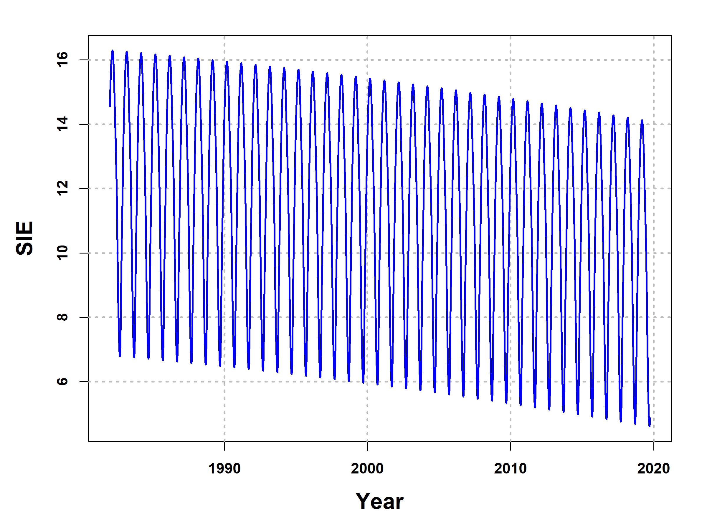
(a)
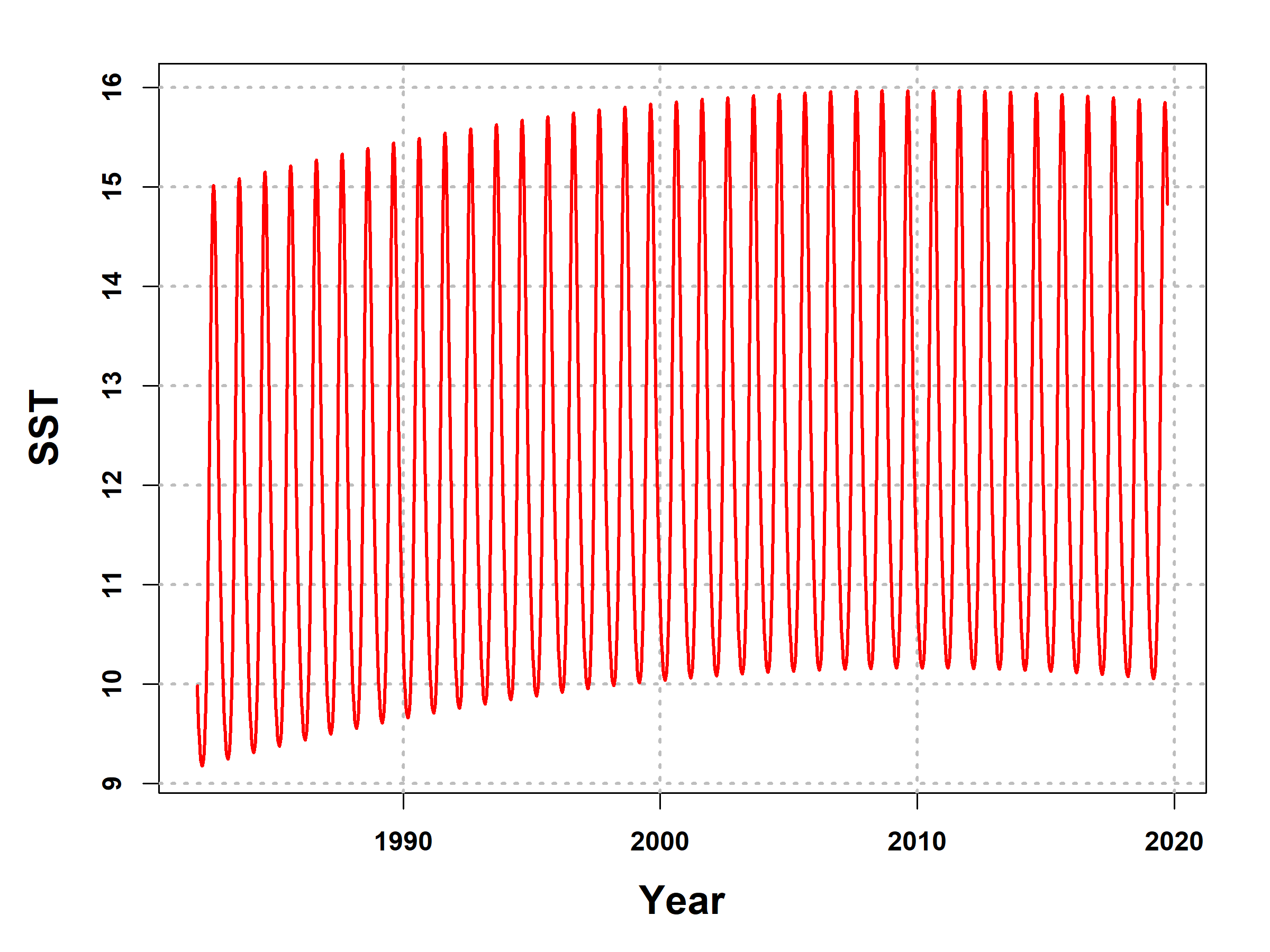
(b)
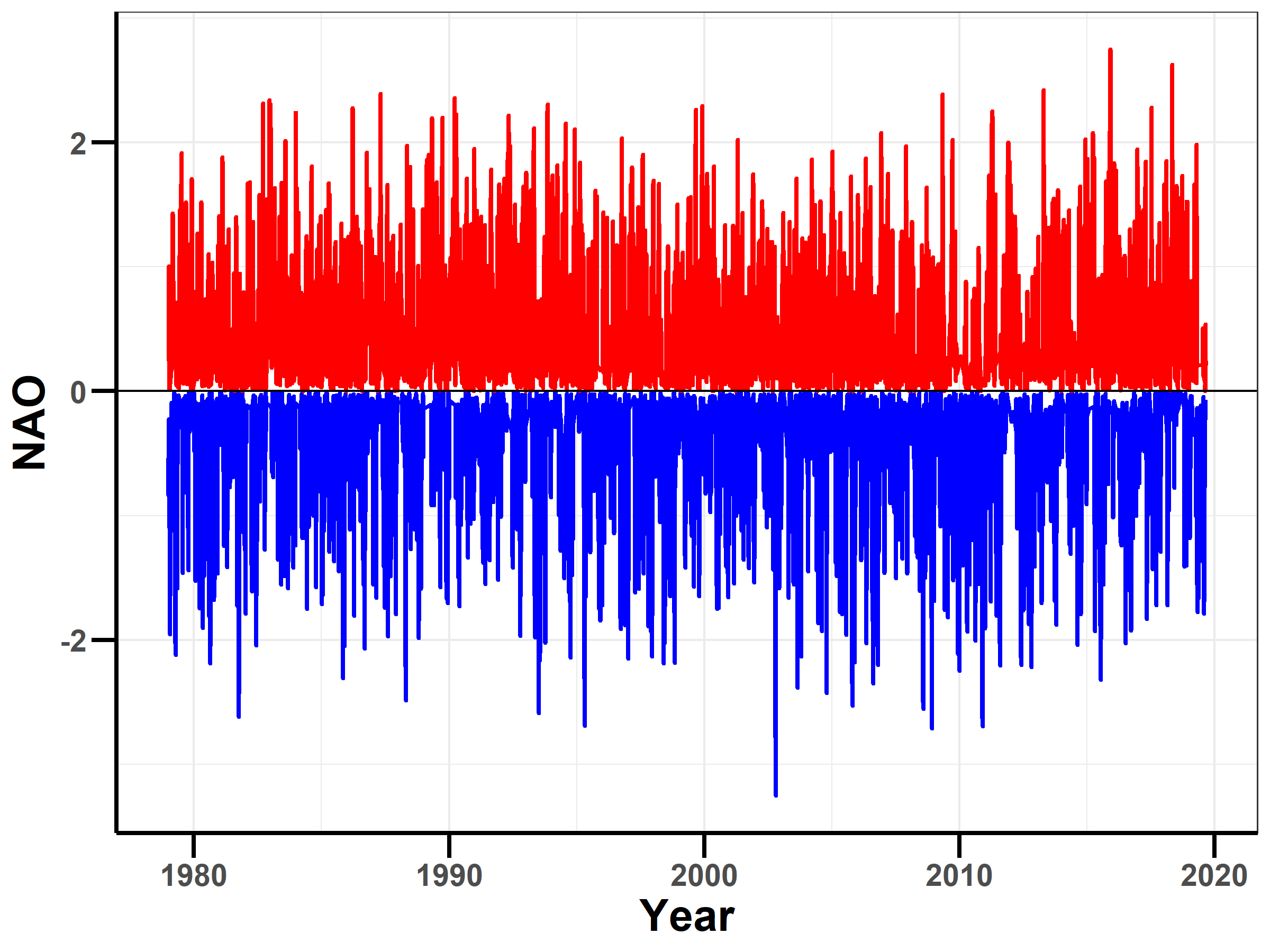
(c)

Figure 1: (a) SIE time series plot from 1982 to 2019. (b) SST time series plot from 1982 to 2019. (c) Plot of the NAO time series over the period of 1979-2019.

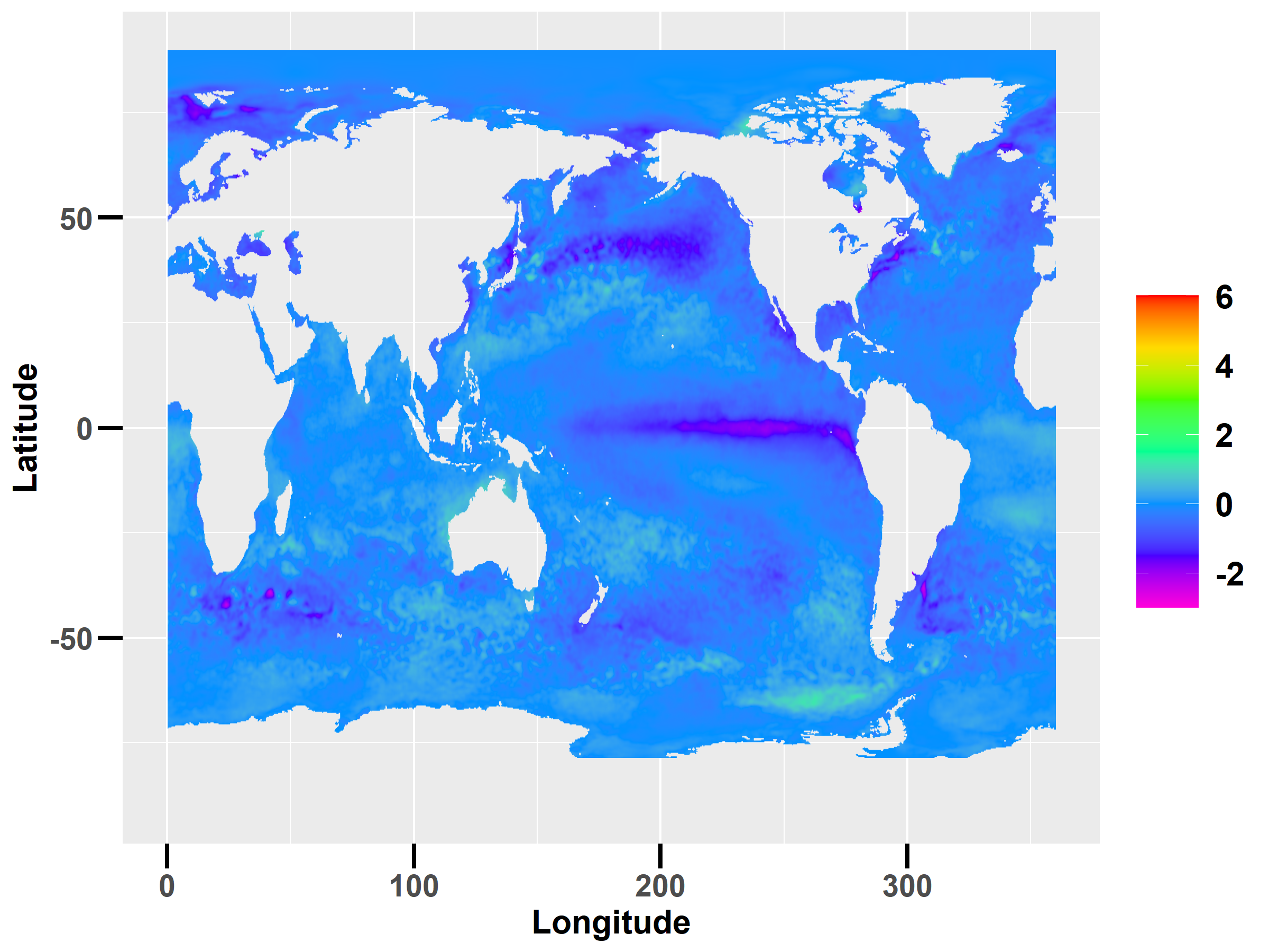
(a)
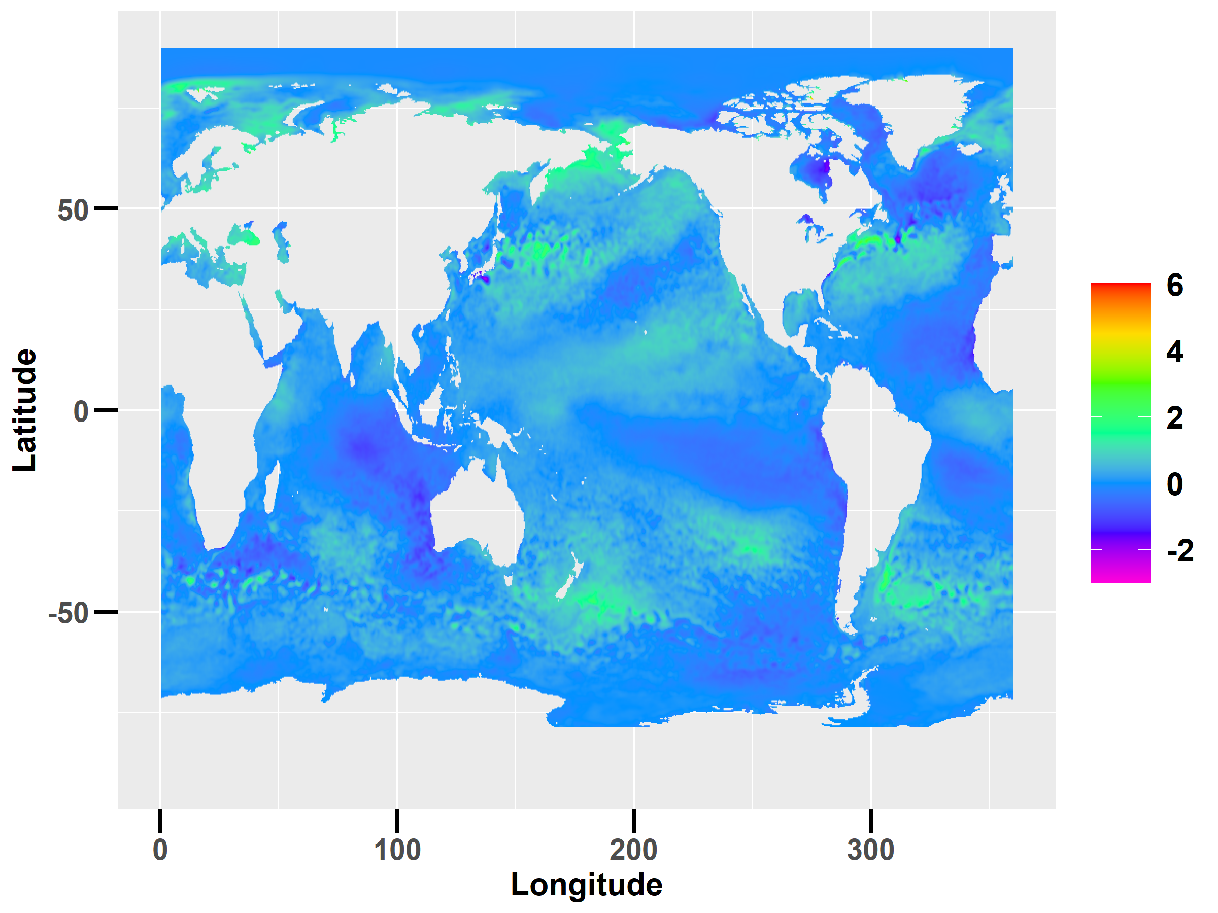
(b)

Figure 2: (a) Grid level $\delta(SST)$ in degree celsius (°C) for 1988 (b) Grid level $\delta(SST)$ in degree celsius (°C) for 2018. The colorbar represents $\delta(SST)$ i.e., the difference between the annual average of SST and the average of all year SST averages at grid level g. In 1988, the majority of grid levels showed $\delta(SST)$ values below 0. However, in 2018, a shift occurred with $\delta(SST)$ exceeding 2 degrees across most grids.

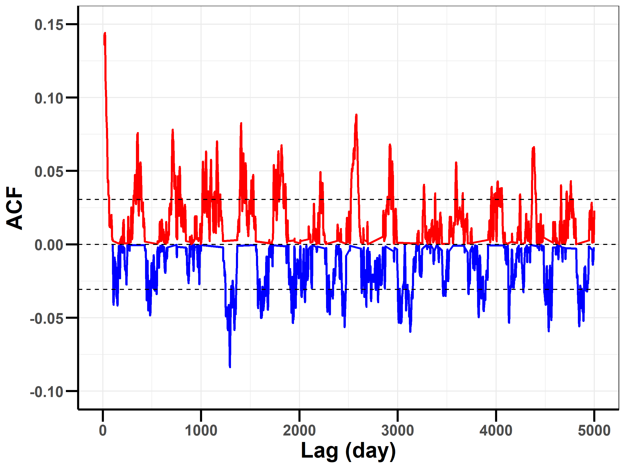
(a)
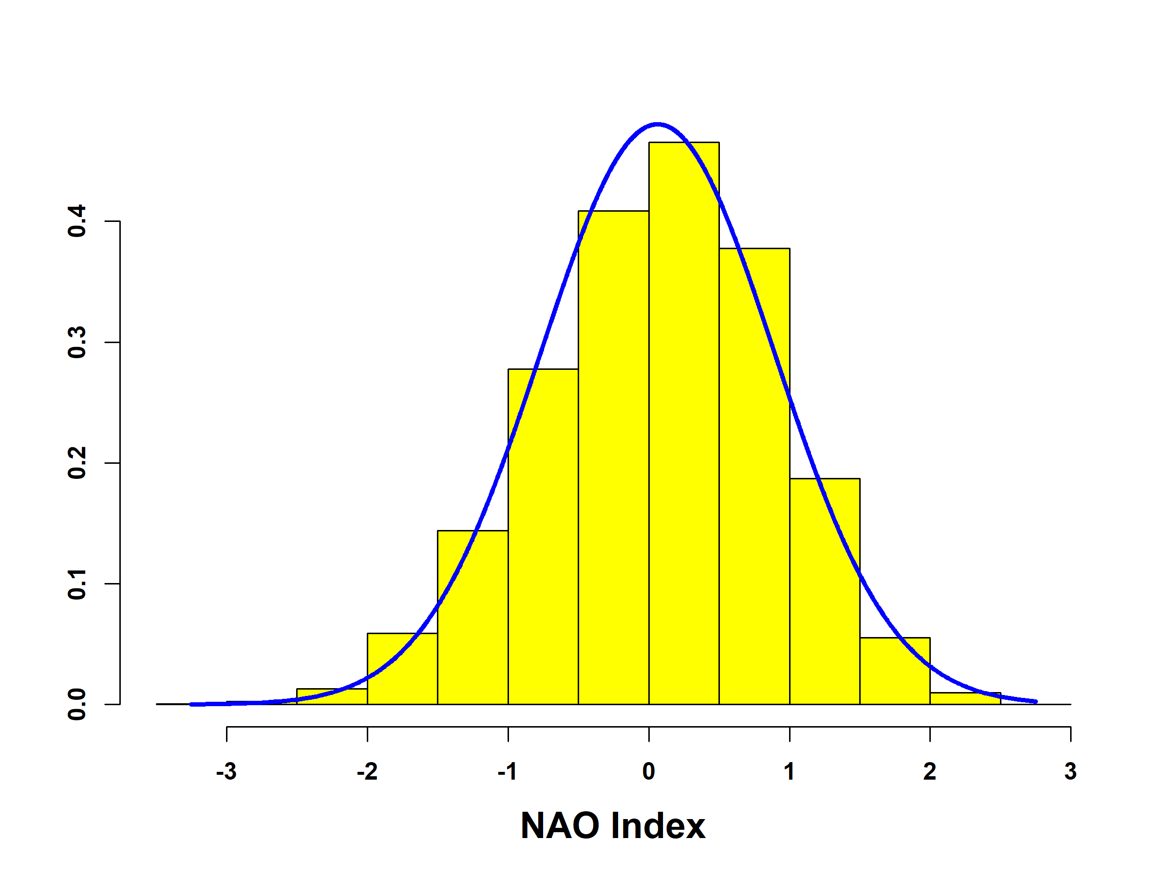
(b)

Figure 3: (a) Autocorrelation plot of NAO with a maximum lag of 5000 days (almost 13 years) indicating the existence of long memory.(b) The NAO index’s marginal probability distribution from 1979 to 2019 is expected to be bell-shaped and symmetric, with zero skewness, reflecting stability. The empirical evidence indicates instability in the system.

Methods	NAO
Simple R/S Hurst estimation	0.73
Corrected R over S Hurst exponent	0.73
Empirical Hurst exponent	0.67
Corrected empirical Hurst exponent	0.66
Theoretical Hurst exponent	0.52

Table 1: The Hurst Exponent value of the NAO index using different methods.

3 Methodology

This section outlines the statistical machine learning (SML) methodology employed to elucidate the feedback loop. Figure (1a,b) illustrates the non-stationary nature of SIE and SST. To address this, we introduce the equations in Section (3.1) and (3.2) that capture the trend and seasonality components of SIE and SST. By detrending the SIE and SST, we obtain the residuals of both variables. These residuals are expected to exhibit characteristics of a zero-mean stationary process. Consequently, we investigate the Granger-causality between the residuals of SIE, residuals of SST, and the North Atlantic Oscillation (NAO). The Granger-causal model employs autoregressive time-series techniques to examine the relationships among these variables [12].

3.1 Modeling Sea Ice Extent

Let us consider $x(t)$ as the SIE at time point $t$. We formulated the modeling of SIE by incorporating both a trend and a seasonal component. The trend component accounts for long-term variations, indicating either an increase or a decrease over time. On the other hand, the seasonal component captures recurring patterns at a fixed and known frequency, based on specific time periods such as the year, week, or day,

$$x(t) = \underbrace{\beta_{0}+\beta_{1}t+\beta_{2}t^{2}}_{trend}+\underbrace{\bigg{\{}\sum_{i=1}^{K}\alpha_{i}\sin(i\omega t)+\sum_{i=1}^{K}\gamma_{i}\cos(i\omega t)\bigg{\}}}_{seasonality}+\epsilon(t),$$ (1)

where $\epsilon$ is error with $\mathbb{E}(\epsilon)=0$, and $Var(\epsilon)=\sigma^{2}$. In the seasonality component, we consider the periodicity with $\omega=\frac{2\pi}{365}$; $\alpha_{i}$ is the coefficient corresponding to the sine of $i^{th}$ harmonics and $\gamma_{i}$ is the coefficient corresponding to the cosine of the $i^{th}$ harmonics. Within the model, we take into consideration $K$ harmonics for each period. Now, two questions arise: (i) How do we determine the appropriate value of $K$? and (ii) When $K$ becomes large, several harmonics may become redundant. To address the first question, we fit the model using various values of $K$ ranging from 1 to $K_{0}$, and select the model with the minimum out-of-sample root mean square error (RMSE). Next, we utilize the least absolute shrinkage and selection operator (LASSO) technique to identify the optimal harmonics in Model (1). The LASSO method selectively retains the harmonics that demonstrate a statistically significant impact in minimizing the error [38]. A similar technique was successfully used to model long-term memory in climate variables [41].

3.2 Modeling Sea Surface Temperature

Let us consider $y(t)$ as the SST at time point $t$. Like SIE, in Equation (1), we formulated the modeling of SST by incorporating both a trend and a seasonal component,

$$y(t) = \underbrace{\tilde{\beta}_{0}+\tilde{\beta}_{1}t+\tilde{\beta}_{2}t^{2}}_{trend}+\underbrace{\bigg{\{}\sum_{i=1}^{K}\tilde{\alpha}_{i}\sin(i\omega t)+\sum_{i=1}^{K}\tilde{\gamma}_{i}\cos(i\omega t)\bigg{\}}}_{seasonality}+\delta(t),$$ (2)

where $\delta$ is error with $\mathbb{E}(\epsilon)=0$, and $Var(\epsilon)=\sigma^{2}$. In the seasonality component, we consider the periodicity with $\omega=\frac{2\pi}{365}$; the component and parameters of the Model (2) have same interpretation as in the Model (1). Therefore, we employ the same strategy to fit the model.

Let us assume that $e(t)$ represents the residual obtained from the best fit of Model (1). Henceforth, we will refer to $e(t)$ as Sea Ice Extent Residuals (SIER). Similarly, $d(t)$ denotes the residual obtained from the best fit of Model (2). Moving forward, we will refer to $d(t)$ as Sea Surface Temperature Residuals (SSTR). It is anticipated that both $e(t)$ and $d(t)$ will exhibit characteristics of zero-mean stationary processes, similar to the North Atlantic Oscillation (NAO). Therefore, our objective is to explore the potential presence of a feedback loop between the SIER, SSTR and NAO by employing the Granger causality test.

3.3 Formulating Feedback Loop with Granger Causality

In order to examine the evolving causal dynamics between SIER and SSTR, and vice versa, we formulate the following hypothesis utilizing the Granger causal models. The full model incorporates the consideration of one variable being influenced by its own historical memory as well as the lagged values of the other two variables. For instance, the NAO variable is modeled as a function of its own lagged values and the lagged value of both SIER and SSTR, i.e.,

$$n(t) = \beta_{0}+\beta_{1}n(t-1)+\cdots+\beta_{k}n(t-k)$$ (3)

$$~{}~{}+\gamma_{1}e(t-1)+\cdots+\gamma_{k}e(t-k)$$

$$~{}~{}+\delta_{1}d(t-1)+\cdots+\delta_{k}d(t-k)+\epsilon(t).$$

Similarly, SIER is modelled as a function of its own lagged values and the lagged value of both NAO and SSTR, i.e.,

$$e(t) = \beta_{0}+\beta_{1}e(t-1)+\cdots+\beta_{k}e(t-k)$$ (4)

$$~{}~{}+\gamma_{1}n(t-1)+\cdots+\gamma_{k}n(t-k)$$

$$~{}~{}+\delta_{1}d(t-1)+\cdots+\delta_{k}d(t-k)+\epsilon(t).$$

Finally, SSTR is modelled as a function of its own lagged values and the lagged value of both NAO and SIER, i.e.,

$$d(t) = \beta_{0}+\beta_{1}d(t-1)+\cdots+\beta_{k}d(t-k)$$ (5)

$$~{}~{}+\gamma_{1}n(t-1)+\cdots+\gamma_{k}n(t-k)$$

$$~{}~{}+\delta_{1}e(t-1)+\cdots+\delta_{k}e(t-k)+\epsilon(t).$$

The Equation (3, 4, 5) collectively form the model depicting the feedback loop between NAO, SIER, and SSTR. To examine the presence of this feedback loop, we conduct the Granger causality test, such as the null hypothesis says that all $\gamma_{i}=0$, i.e.,

$$H_{0}:\gamma_{1}=\cdots=\gamma_{k}=0~{}~{}~{}\text{and}~{}~{}~{}~{}\delta_{1}=\cdots=\delta_{k}=0,$$ (6)

to reject the null hypothesis in our alternate hypothesis we have to check if at least one $\gamma_{i}~{}~{}\text{or}~{}~{}\delta_{i}\neq 0$, i.e.,

$$H_{1}:\text{at least one }\gamma_{i}\neq 0~{}~{}~{}\text{or}~{}~{}~{}~{}\delta_{i}\neq 0.$$ (7)

We run this test for all three models, and if all three tests are rejected, it confirms the existence of the feedback loop.

3.4 Dynamic Statistical Approach

Kolstad [19] has criticized the statistical models for climate research, citing the reason that the relationship between the predictor and dependent variable did not change over time (i.e., regression coefficients remained constant over time). Here, we take into account this criticism by constructing a Bayesian Dynamic Linear Model, along the line of the work by [10], where the relationship between a predictor and the dependent variable is updated over time by updating the coefficients. First, we consider the first derivative (momentum) and second derivative (acceleration) of the model presented in the above Equation (1) are:

$$x^{\prime}(t) = \underbrace{\beta_{1}+2\beta_{2}t}_{trend}+\underbrace{\omega\bigg{\{}\sum_{i=1}^{K}\alpha_{i}\cos(i\omega t)-\sum_{i=1}^{K}\gamma_{i}\sin(i\omega t)\bigg{\}}}_{seasonality}+\epsilon_{1}(t)$$ (8)

$$x^{\prime\prime}(t) = \underbrace{2\beta_{2}}_{trend}+\underbrace{\omega^{2}\bigg{\{}\sum_{i=1}^{K}\alpha_{i}\sin(i\omega t)+\sum_{i=1}^{K}\gamma_{i}\cos(i\omega t)\bigg{\}}}_{seasonality}+\epsilon_{2}(t),$$ (9)

where $\epsilon_{1}$ and $\epsilon_{2}$ are noises corresponding to momentum and acceleration signal. Then we developed the Bayesian dynamic linear models (BDLM) for NAO as follows:

$$n_{t} = \beta_{0t}+\beta_{1t}n_{t-1}+\gamma_{1t}x^{\prime}_{t-1}+\epsilon_{t},$$ (10)

$$\beta_{0t} = \rho_{0}\beta_{0,t-1}+\eta_{1t},$$ (11)

$$\beta_{1t} = \rho_{1}\beta_{1,t-1}+\eta_{2t},,$$ (12)

$$\gamma_{1t} = \rho_{2}\gamma_{1,t-1}+\eta_{3t},$$ (13)

where Equation (10) is known as observation equation; and Equation (11, 12,13) are known as the system equations; the $n_{t}$ is NAO at time point $t$; the $x^{\prime}_{t}$ is the momentum of SIE at time point $t$; $\epsilon_{t}$ is white noise follows $N(0,\sigma_{\epsilon}^{2})$; $\eta_{jt},~{}j=1,2,3$ are white noise associated with system equation follows $N(0,\sigma_{\eta_{j}}^{2})$. Note that $\rho=(\rho_{0},\rho_{1},\rho_{2})$ should be bounded, that is, $|\rho_{j}|<1$, such that the model would be a stationary process like the NAO index. We know that NAO is a mean stationary process; see Figure (1c); hence this restriction of $\rho_{j}$ is required. We present the Equation (10) and Equation (11,12,13) in the matrix notations as follows:

$$Y_{t} = X_{t}\beta_{t}+\epsilon_{t},~{}~{}~{}~{}\text{observation ~{}equation},$$

$$\beta_{t} = R\beta_{t-1}+\eta_{t},~{}~{}~{}~{}\text{system~{} equation},$$ (14)

where $\epsilon_{t}\sim N(0,\sigma^{2})$, and $\eta_{t}\sim N(0,Q)$. The Bayesian update solution (aka., Kalman filter) for Equation (14) can be taken from [10, 35], as follows

$$K_{t} = R\Sigma_{t}X_{t}^{T}(X_{t}\Sigma_{t}X^{T}+\sigma^{2})^{-1},$$

$$\hat{\beta}_{t+1} = R\hat{\beta}_{t}+K_{t}(Y_{t}-X_{t}\hat{\beta}_{t}),$$ (15)

$$\Sigma_{t+1} = R\Sigma_{t}R^{T}-K_{t}X_{t}\Sigma_{t}R^{T}+Q.$$

In this study, BDLM corresponds to the Equation (1) developed. These models are then updated by the BDLM using a Kalman filter, as presented in Equation (15). Through these Kalman updates, $\beta$ coefficients are dynamically updated. The model for SIE is as follows:

$$x(t) = \beta_{0}(t)+\beta_{1}(t)\sin(\omega t)+\gamma_{1}(t)\cos(\omega t)+\epsilon,$$ (16)

where $x(t)$ is SIE extent at time point $t$; $\beta_{0}(t)$, $\beta_{1}(t)$ and $\gamma_{1}(t)$ are the dynamic coefficients, updated via Kalman update Equation (15). Note that the model does not have any trend part because if there is any trend in the data, that will be captured automatically in the coefficients. In addition, the BDLM was built in the following way:

$$n(t) = \beta_{0}(t)+\sum_{k=1}^{K}\beta_{k}(t)n(t-1)+\sum_{k=1}^{K}\gamma_{k}(t)n(t-k)+\epsilon(t),$$ (17)

where $n(t)$ is NAO and $x^{\prime}(t-k)$ is the momentum of the SIE at ($t-k$). Here, the Akaike information criterion type model selection process was used to obtain the optimal choice for the model Equation (17). It may be noted that if the model’s coefficients are static, then the Granger causal model is a special case of Equation (17).

4 Analyses and Results

4.1 Analyses of SIER, SSTR, and NAO

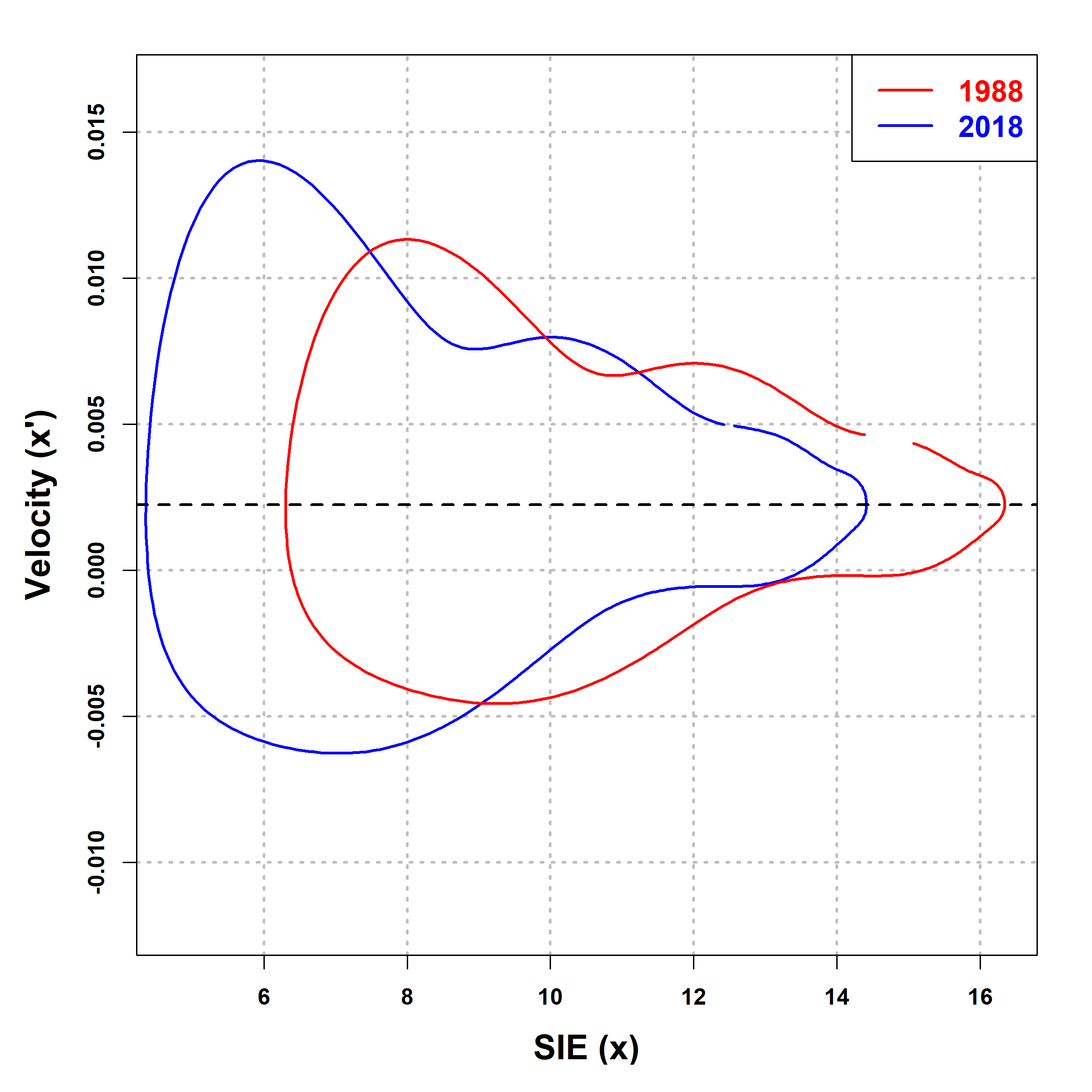
(a)
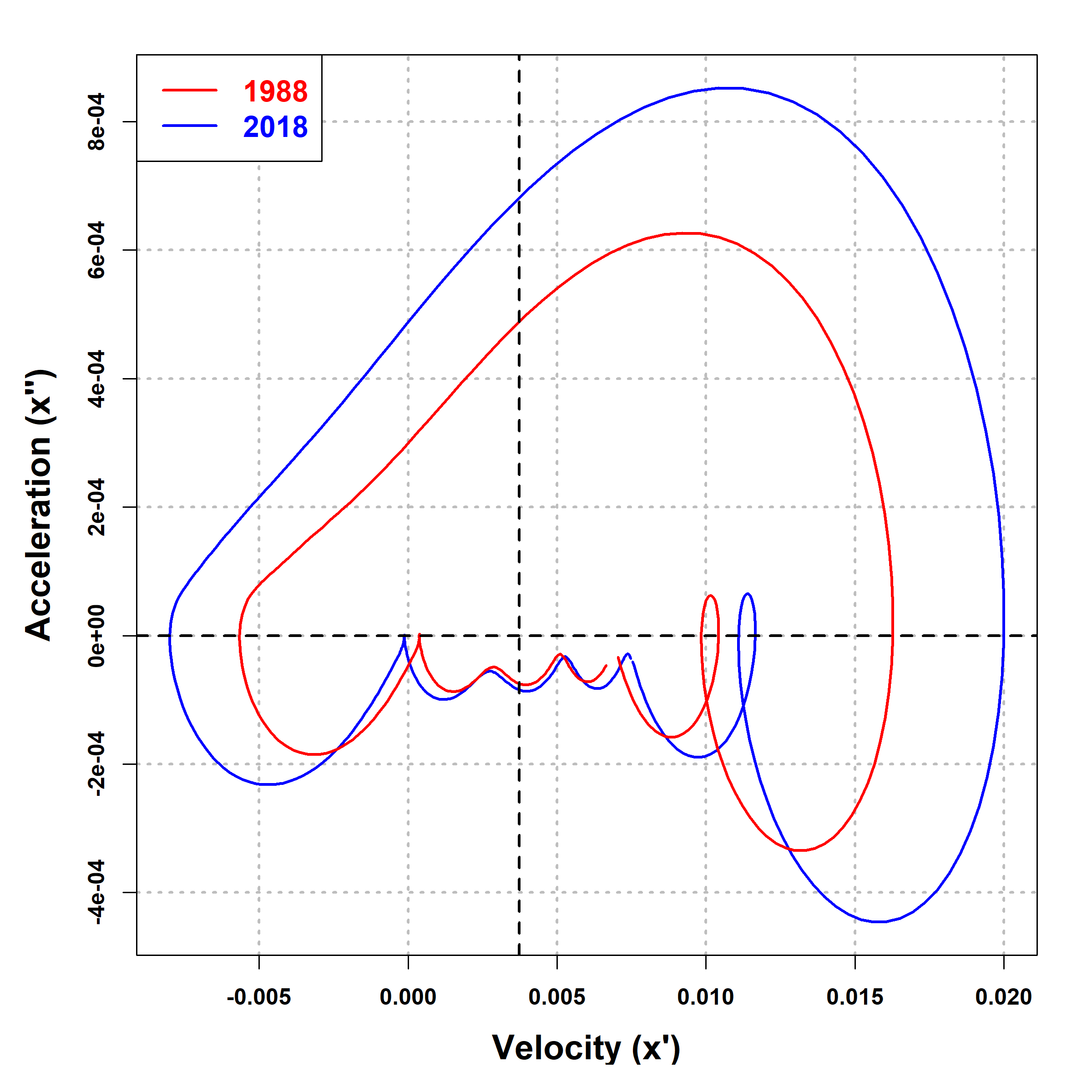
(b)

Figure 4: (a) Phase-line plot of SIE ($x(t)$ as per Equation (1) vs. velocity of SIE ($x^{\prime}(t)$ as per Equation (8) for the two years 1988 and 2018. (b) The phase-plane plot of the velocity of SIE ($x^{\prime}(t)$ as per Equation (8) vs. acceleration of SIE ($x^{\prime\prime}(t)$ as per Equation (9) for the two years 1988 and 2018.

The modeling framework pertaining to SIE and SST is detailed in sections (3.1) and (3.2). In Figure 4(a,b), which illustrates the phase-plane analysis of SIE, noticeable fluctuations in both the spatial extent and the rate of volume change of SIE become apparent. These figures portray the dynamic interplay through variations in the phase-line distribution, represented by the expanding area beneath the paired curves. Furthermore, a significant increase in the rate of sea ice melting between 1988 and 2018 becomes evident, an outcome attributed to the phenomenon of melting SIE.

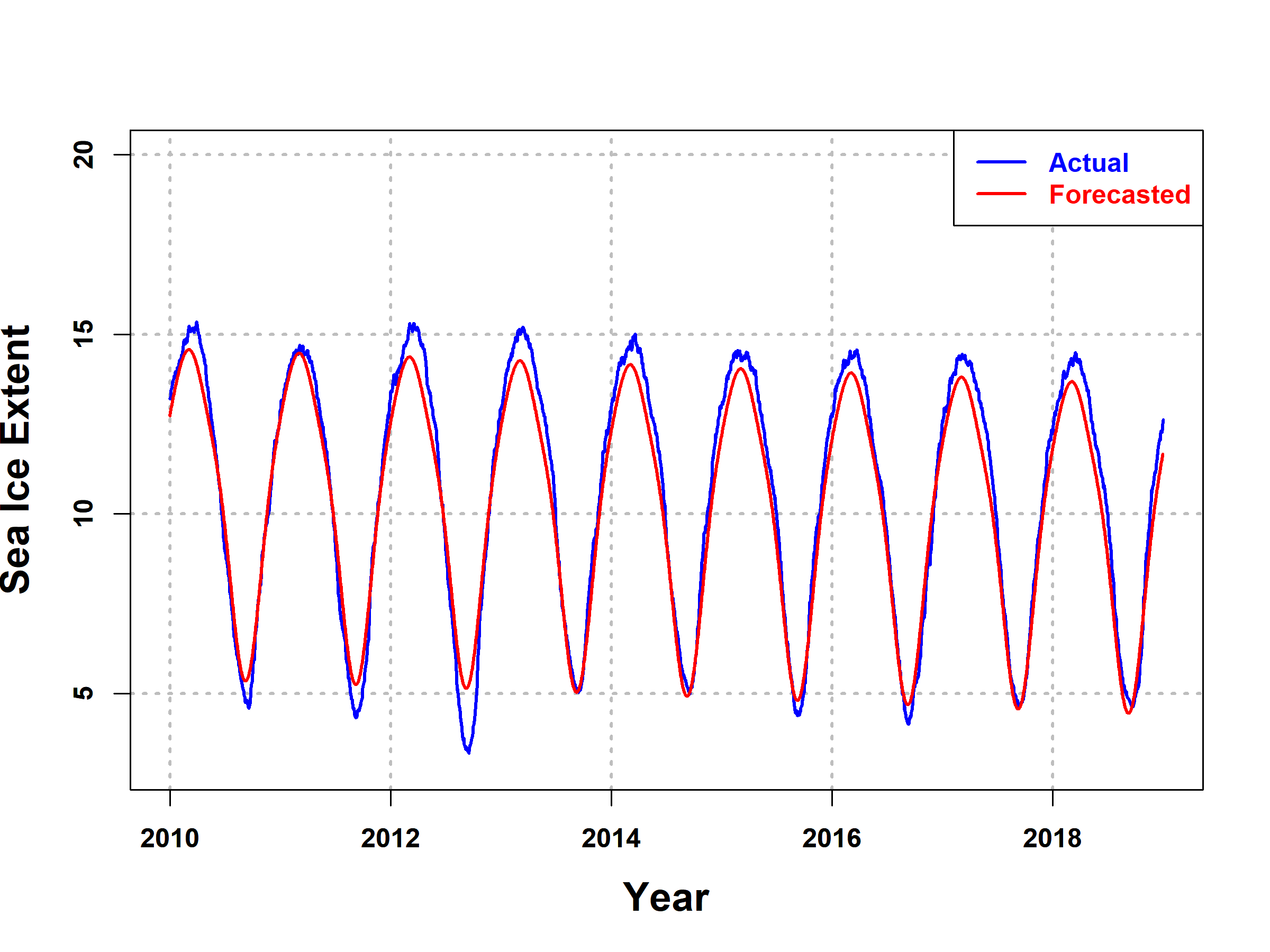
Figure 5: To evaluate the effectiveness of our proposed model (Equations (1,8,9)), a machine learning assessment was carried out. The training dataset spanned from 1979 to 2009, while the test dataset encompassed the years 2010 to 2019.

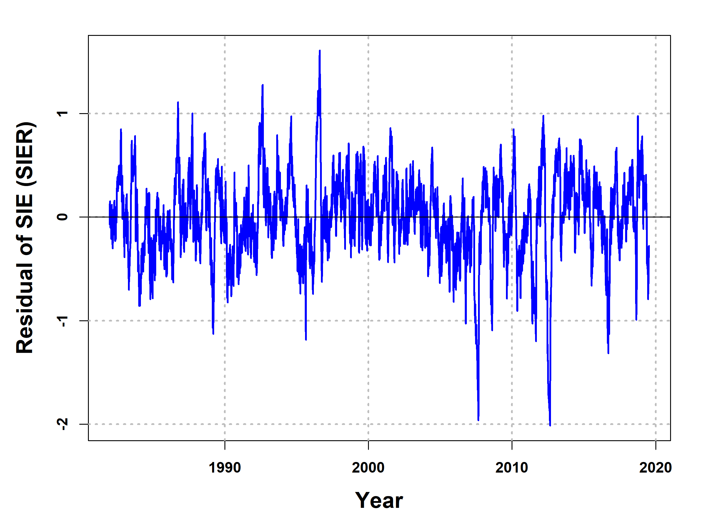
(a)
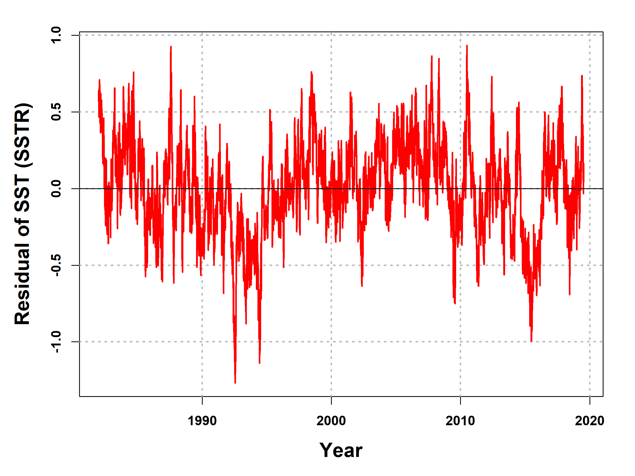
(b)

Figure 6: Time series plots of (a) Residual of SIE (SIER) (b) Residual of SST (SSTR)

Moving on to Figure (5), a visualization of the projected and observed trajectories within the test dataset spanning from 2010 to 2019 is presented. Root Mean Square Error (RMSE) values are computed for both the training and test datasets, yielding an RMSE value of 0.36 for the training set and 0.41 for the test set. This underscores the model’s robust capacity for generalization in out-of-sample scenarios, as indicated by the high R-squared value of 0.9865. The time series plot for SIER and SSTR is portrayed in Figure (6). Notably, both processes exhibit the characteristic of being mean zero stationary, which is a fundamental requirement for conducting the Granger causal test.

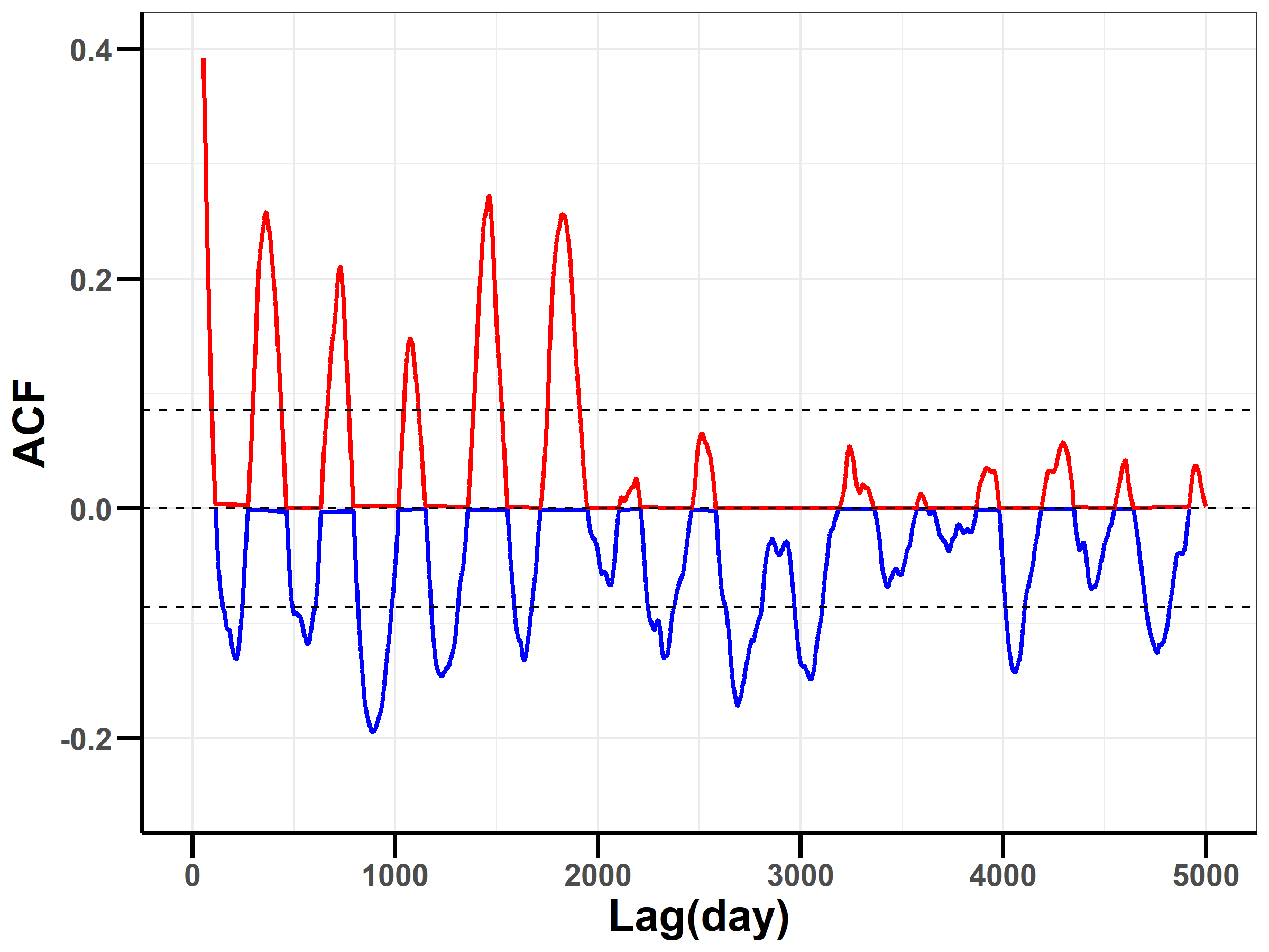
(a)
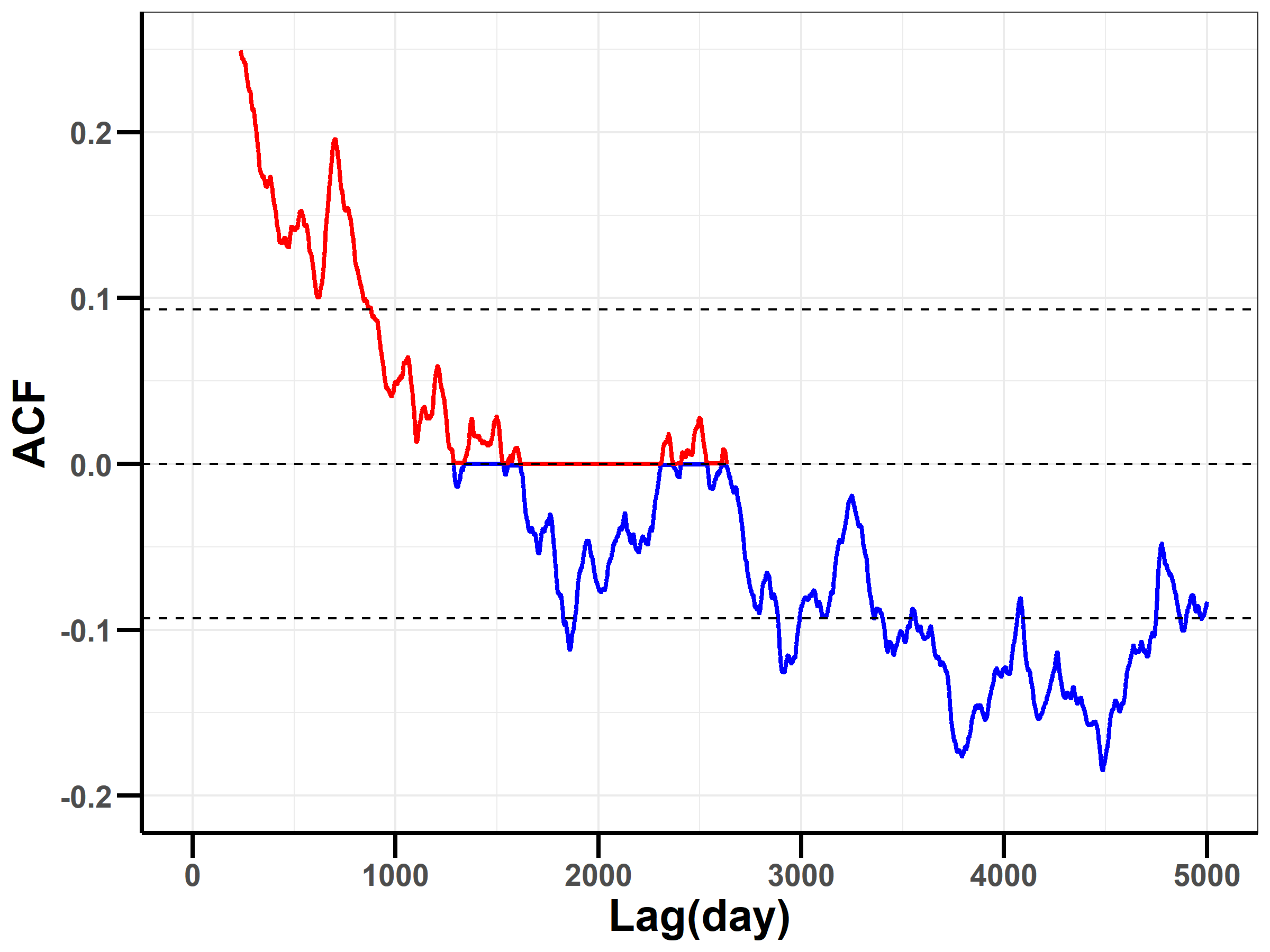
(b)

Figure 7: ACF plots of (a) Residual of SIE (SIER) (b) Residual of SST (SSTR)

Figure (7) and Table (2) jointly demonstrate the presence of long memory in SIER and SSTR. This inference is substantiated by the significantly elevated Hurst exponent values, exceeding the threshold of 0.5, thus reflecting the underlying memory dynamics in these processes. The correlation matrix for NAO, SIER, and SSTR is presented in Table (3), calculated over a span of 38 years from January 1982 to September 2019. Enclosed within parentheses are the associated P-values, which offer insights into the statistical significance of these correlations. Particularly noteworthy is the robust and statistically significant correlation between SSTR and NAO. Furthermore, a strong correlation is evident between SIER and SSTR. However, it is important to note that the correlation between NAO and SIER appears to be relatively weaker in significance.

4.2 Granger Causal Test

We delve into the examination of the positive feedback loop. The Granger causal models are formulated with null and alternative hypotheses, as depicted in Equations (6) and (7). The null hypothesis asserts that all $\gamma_{i}$ coefficients are equal to zero, thereby establishing $H_{0}:\gamma_{1}=\cdots=\gamma_{k}=0$. In contrast, the alternative hypothesis $H_{1}$ aims to reject this by examining whether at least one $\gamma_{i}$ deviates from zero. Table (4) presents the ANOVA F-test outcomes for the Granger causal models outlined in Equations (3), (4), and (5).

The ANOVA F-test ($\text{p-value}=0.0178$) effectively refutes the null hypothesis, indicating that SSTR and SIER indeed exert a Granger-causal influence on NAO. Similarly, the ANOVA F-test ($\text{p-value}=2.16\times 10^{-6}$) dismisses the notion that NAO and SIER lack a Granger-causal impact on SSTR. Likewise, the ANOVA F-test ($\text{p-value}=2.17\times 10^{-10}$) rejects the null hypothesis that NAO and SSTR do not possess a Granger-causal effect on SIER. These compelling outcomes collectively confirm the existence of a feedback loop connecting SIER, SSTR, and NAO.

Continuing, the analysis we employ an Akaike information criterion-based model selection process, and we identify the optimal configuration for the Model Equation (17). Notably, if the model coefficients were static, the Granger causal model would represent a special case of Equation (17).

The synthesis of these revelations underscores the presence of a reciprocal feedback loop among NAO, SIER, and SSTR. Subsequently, we move forward to demonstrate the affirmative nature of this loop. Emphasizing the skewness of NAO in Table (5), we offer insight into the bootstrap confidence intervals (C.I.) across different time intervals—daily, weekly, and monthly. In a scenario of stable NAO, a skewness value of zero is expected. However, our findings unveil a negatively skewed distribution, indicating a statistically significant departure from stability. This pronounced outcome vividly underscores the prevailing instability within the NAO dynamics.

Together, these analyses substantiate the existence of a complex feedback loop among NAO, SIER, and SSTR. This discovery not only expands our understanding of climate interdependencies but also reveals a distinctive form of instability inherent within the North Atlantic system.

4.3 Dynamic Statistical Approach

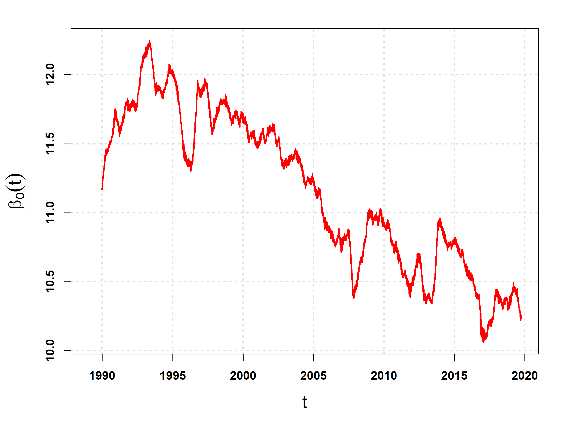
(a)
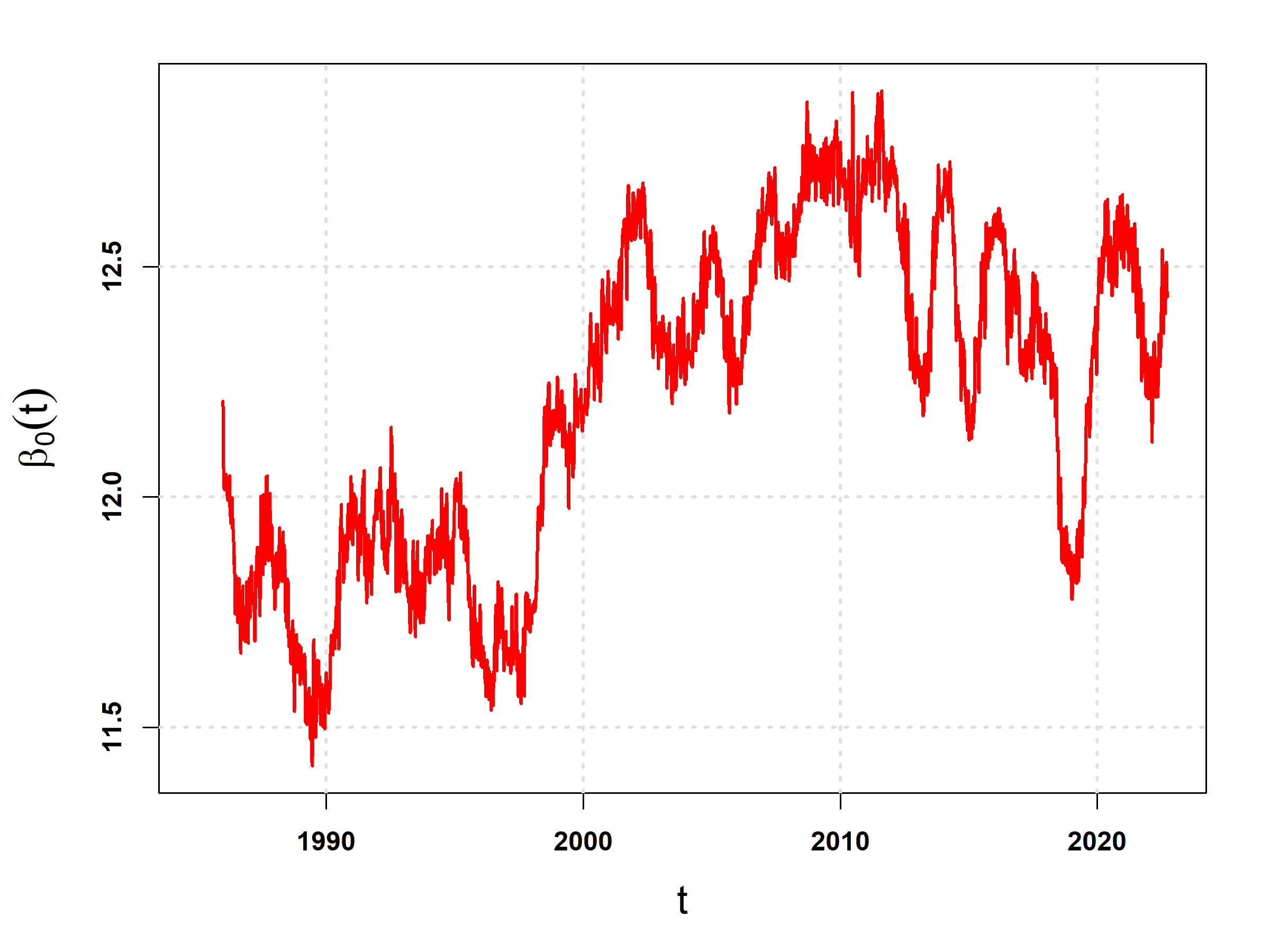
(b)
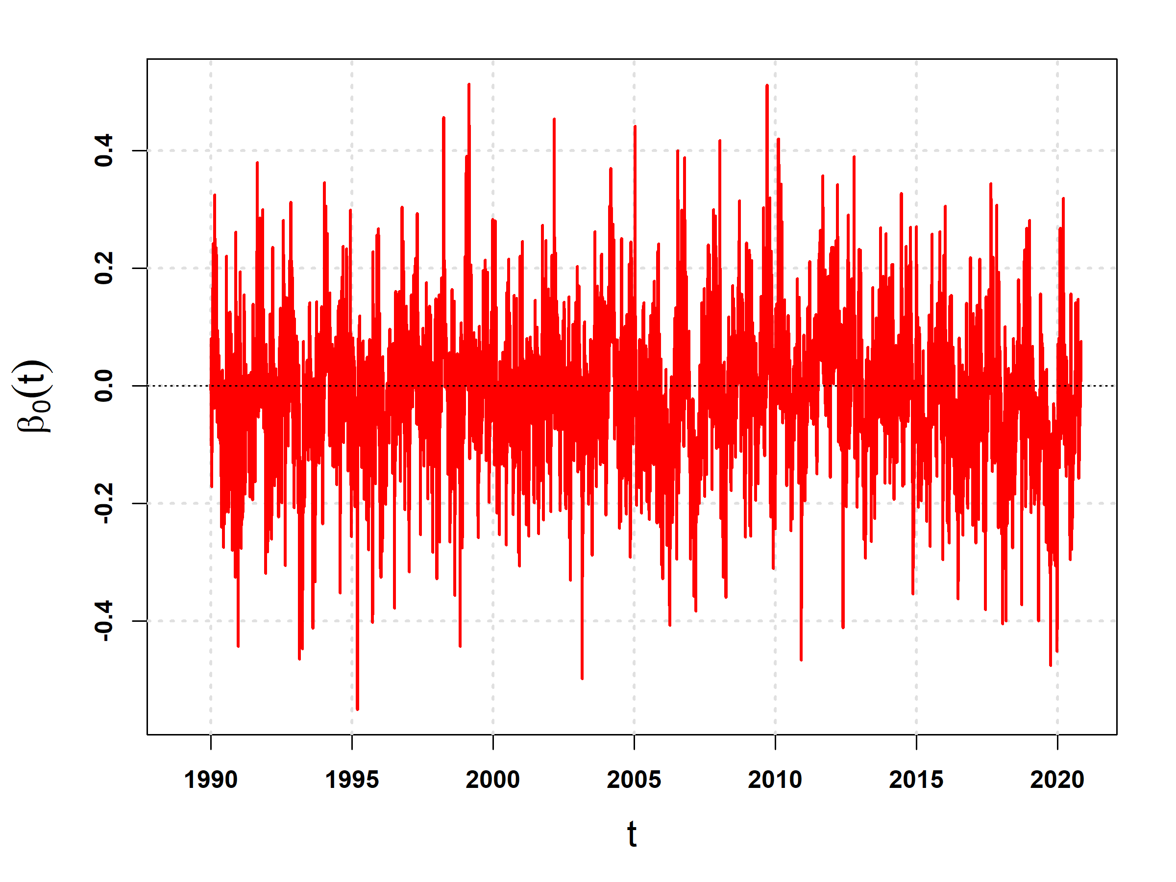
(c)
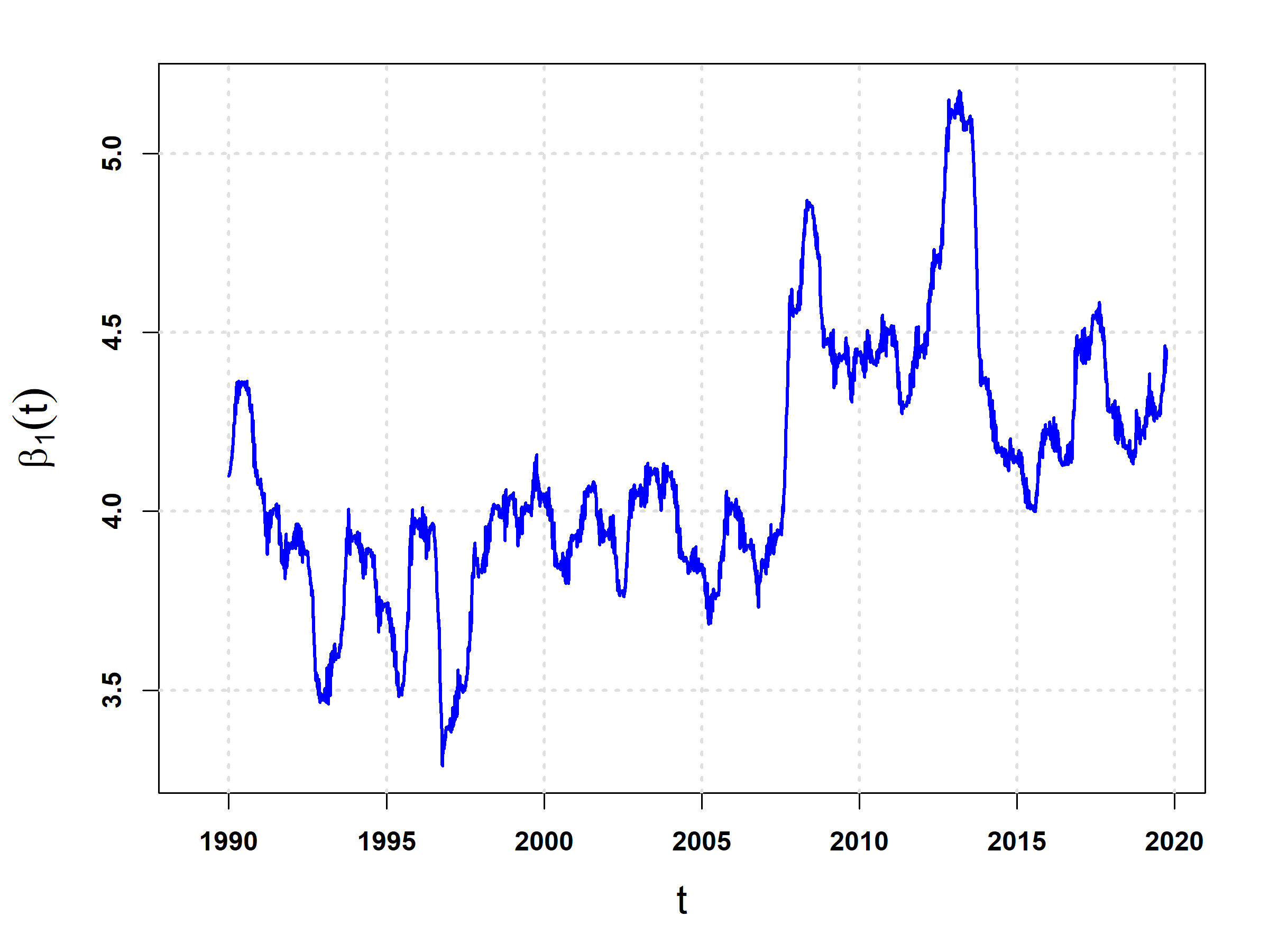
(d)
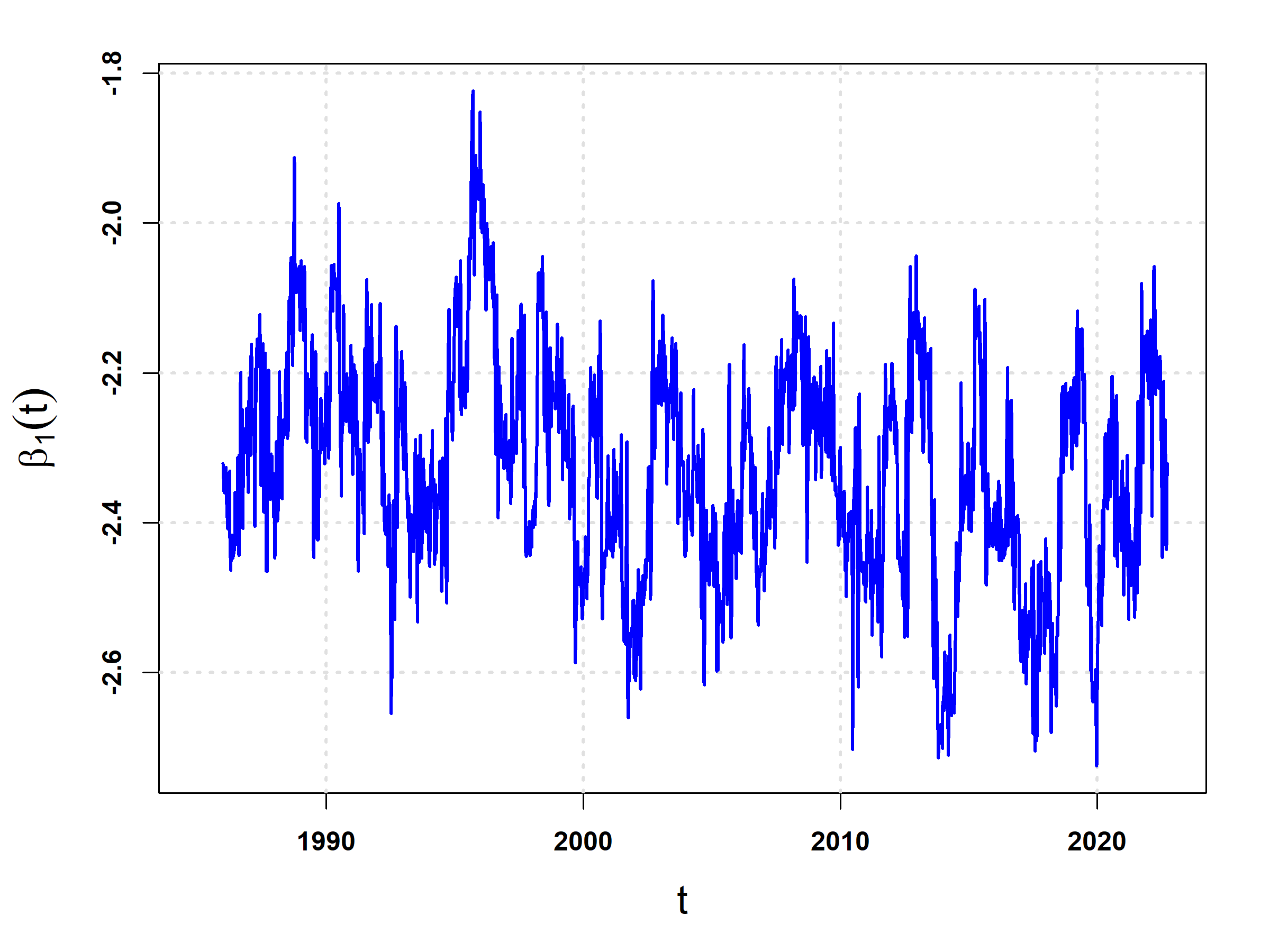
(e)
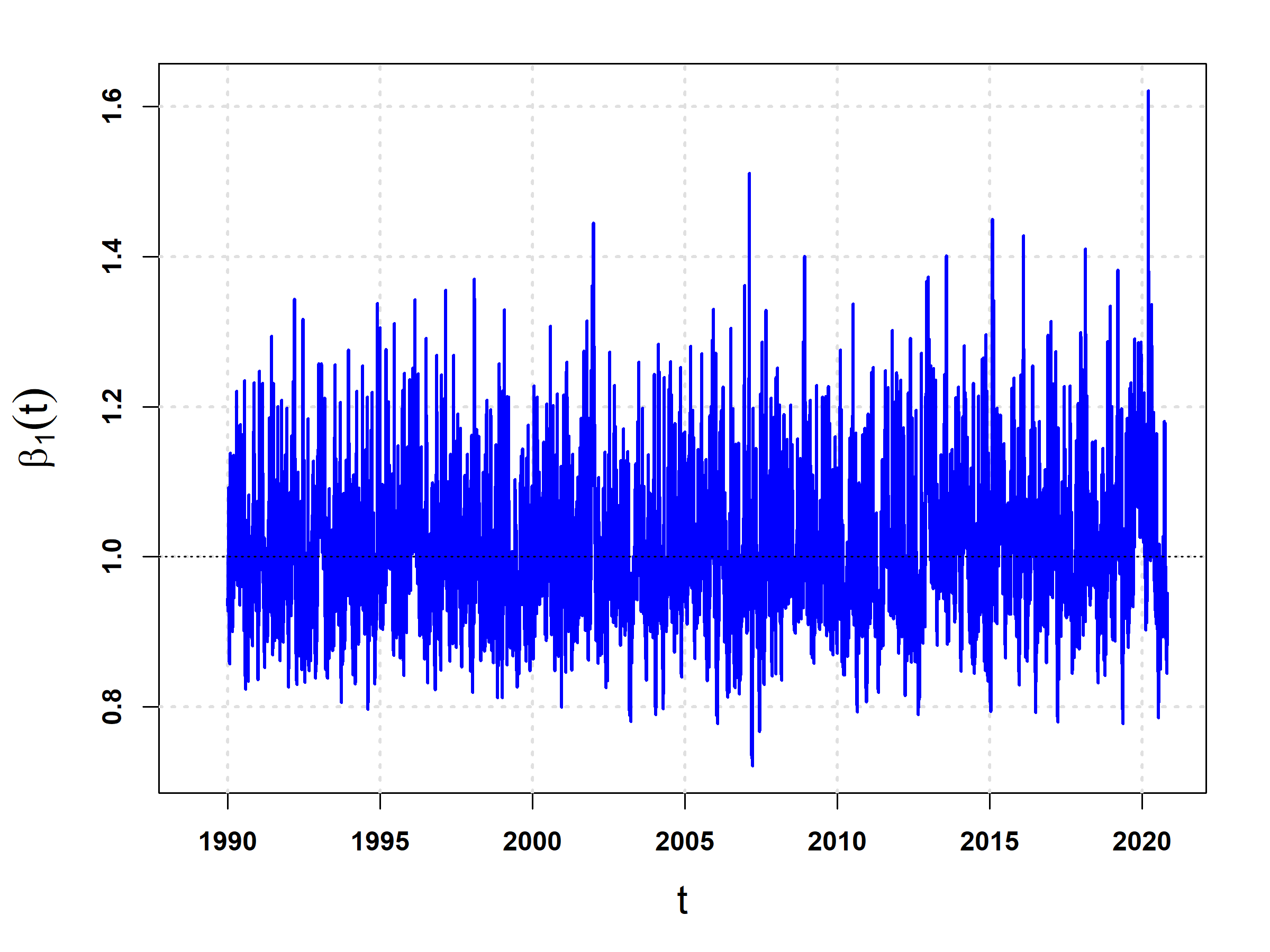
(f)
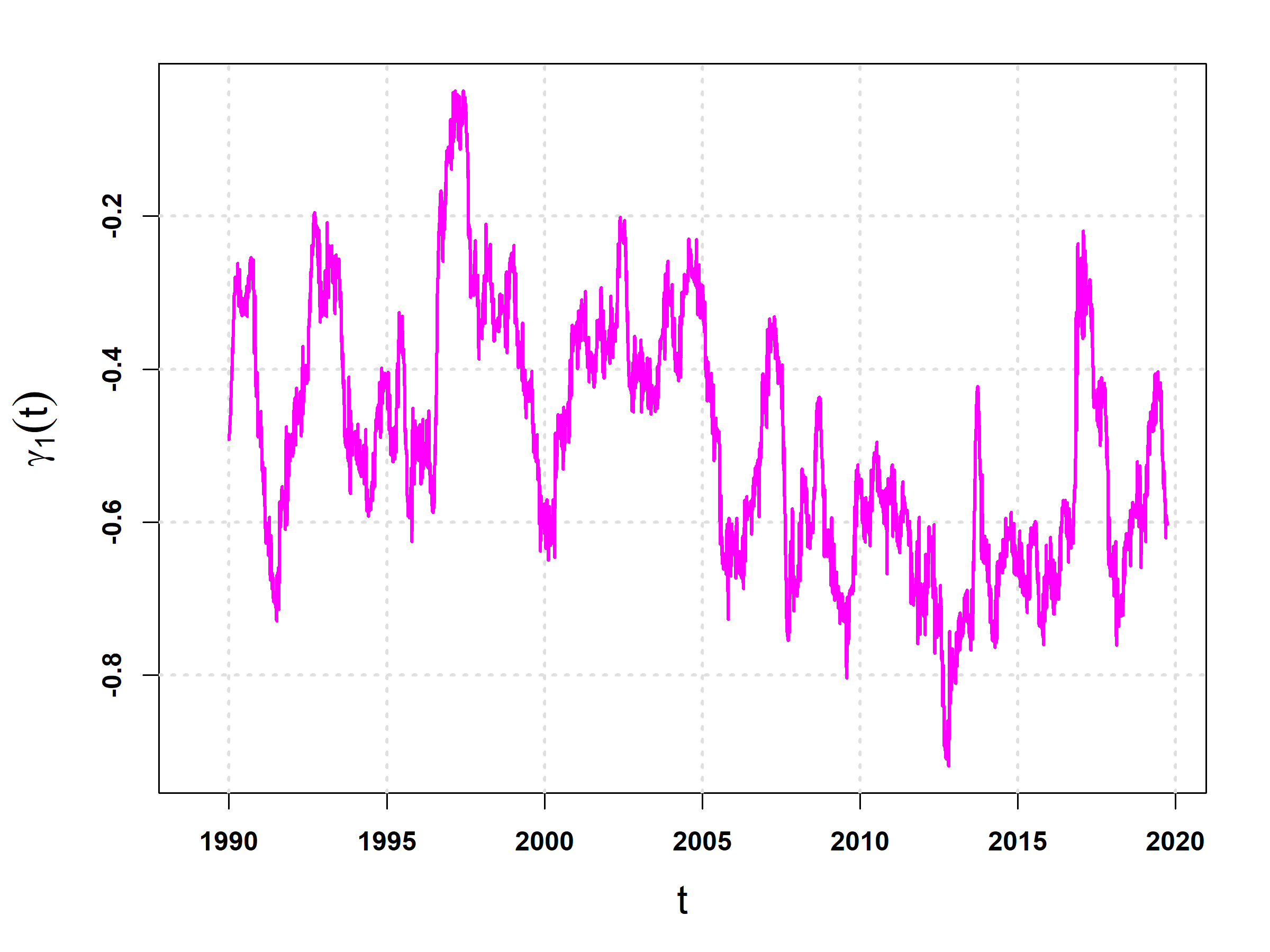
(g)
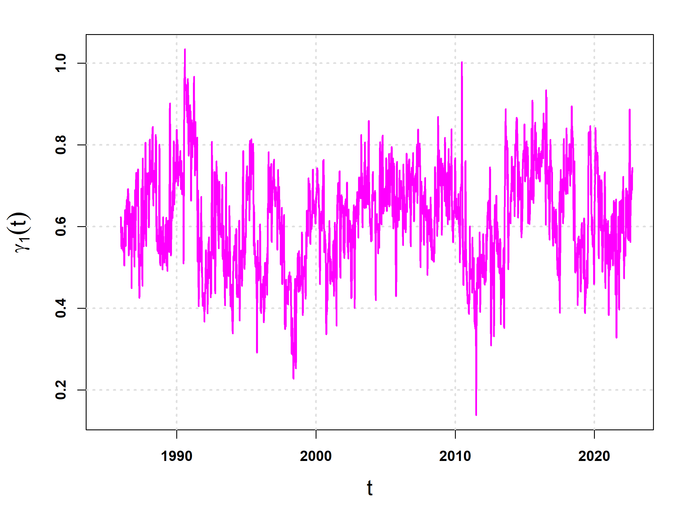
(h)
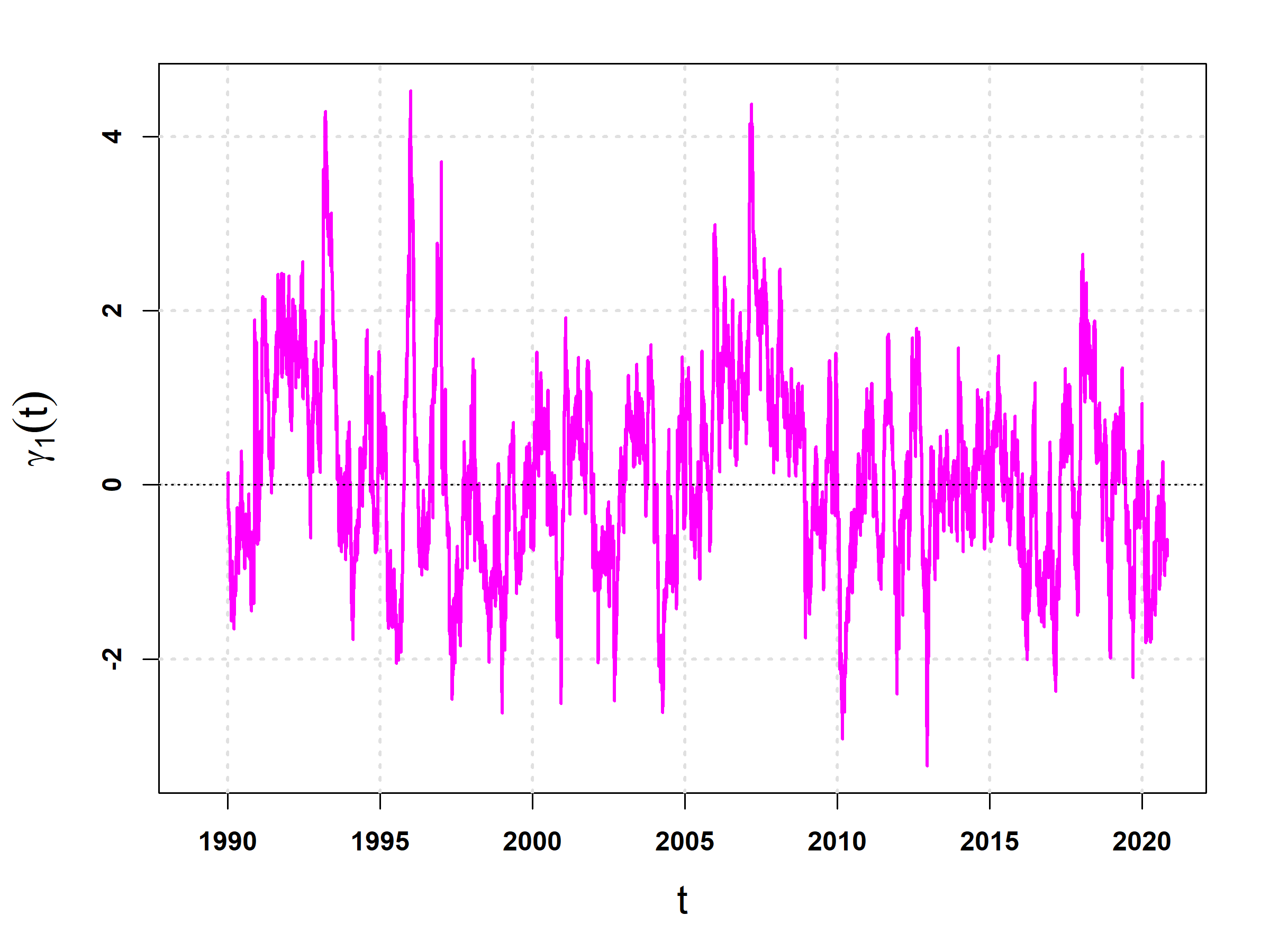
(i)

Figure 8: (a) The downward trend in the dynamic intercept $\beta_{0}(t)$ of SIE indicates that the SIE is shrinking over time. (b) The downward trend in the dynamic intercept $\beta_{0}(t)$ of SST indicates an increasing trend in SST. (c) The dynamic intercept $\beta_{0}(t)$ of NAO is the mean-zero stationary process like NAO($t$). (d) The dynamic coefficient $\beta_{1}(t)$ corresponding to $\sin{\omega t}$ for SIE($t$). (e) The dynamic coefficient $\beta_{1}(t)$ corresponding to $\sin{\omega t}$ for SST($t$). (f) The dynamic coefficient $\beta_{1}(t)$ corresponding to $NAO(t-1)$ for $NAO(t)$. (g) The dynamic coefficient $\gamma_{1}(t)$ corresponding to $\cos{\omega t}$ for SIE($t$). (h) The dynamic coefficient $\gamma_{1}(t)$ corresponding to $\cos{\omega t}$ for SST($t$). (i) The dynamic coefficient $\gamma_{1}(t)$ corresponding to SST($t$) for NAO($t$).

In Figure (8a), the diminishing trajectory of the dynamic intercept $\beta_{0}(t)$ for SIE signifies a gradual decline in SIE over time. Correspondingly, Figure (8b) highlights the ascending trend of the dynamic intercept $\beta_{0}(t)$ for SST, indicating a progressive increase in SST. Transitioning to Figure (8c), the dynamic intercept $\beta_{0}(t)$ for NAO represents a mean-zero stationary process akin to NAO($t$).

Further exploration unveils Figure (8d), illustrating the dynamic coefficient $\beta_{1}(t)$ in harmony with $\sin{\omega t}$ for SIE($t$). Similarly, Figure (8e) elucidates the dynamic coefficient $\beta_{1}(t)$ corresponding to $\sin{\omega t}$ for SST($t$). In Figure (8f), the portrayal of the dynamic coefficient $\beta_{1}(t)$ pertains to $NAO(t-1)$ in relation to $NAO(t)$.

Additionally, Figures (8g), (8h), and (8i) provide insights into the dynamic coefficients $\gamma_{1}(t)$ associated with $\cos{\omega t}$ for SIE($t$), SST($t$), and NAO($t$), respectively.

Common criticisms of traditional statistical models often underscore the assumption of static relationships between predictors and dependent variables over time [19]. To counter this limitation, our study adopts a BDLM as detailed in Section 3.4, drawing inspiration from previous works [33, 27]. This innovative approach ensures an adaptive update of the predictor-dependent variable relationship as time unfolds (see Figure (8)).

Furthermore, echoing the findings of [19], our study substantiates a lagged correlation between NAO and SIE within the Barents-Kara Sea. Remarkably, our research extends beyond this region to encompass the broader North Atlantic and Arctic area, thereby broadening the scope of the observed relationship.

Overall, our methodology not only addresses the limitations of conventional statistical models but also enriches our understanding of the evolving relationships between key climate variables within the dynamic context of the North Atlantic region.

5 Concluding Remarks

In conclusion, this study delved into the intricate dynamics and identified critical instability driven by positive feedback loops among three pivotal climate variables: melting SIE, rising SST, and the NAO. Employing a generic approach rooted in statistical machine learning, we pursued a comprehensive analysis that offers valuable insights into climate variability and its implications for the North Atlantic region.

Unlike intricate climate forecast models, our methodology embraced a less computationally intensive yet more universal strategy, facilitating an all-encompassing examination across the vast North Atlantic area. Addressing a central critique highlighted by Kolstad[19], our BDLM dynamically updated the predictor-dependent variable relationship, enabling us to overcome static model limitations.

The study’s major revelations are noteworthy: (i) a reciprocal Granger causality between SIE and SST, (ii) a mutual Granger causality between SST and NAO, and (iii) an anti-correlation between SST and NAO. This anti-correlation implies that the increasing SST trend is likely to trigger increased occurrences of negative NAO. This aligns with our intriguing finding that the NAO index exhibits negative skewness at various time scales (daily, weekly, and monthly), contrary to its expected mean-zero stationary behavior.

Importantly, the negative skewness of the NAO index, despite its mean-zero stationary nature, signals an impending critical instability. This unsettling phenomenon suggests an elevated probability of negative NAO occurrences, foretelling increased bouts of frigid climates in the North Atlantic region, particularly affecting northern Europe and eastern North America. This realisation underscores the significance of this study in predicting a notable climate transformation.

Overall, this research contributes substantively to the understanding of critical instability within intricate climate systems. Leveraging statistical machine learning techniques, our study enhances our grasp of the dynamic interplay among vital climate variables, extending our insights into the intricate mechanisms that shape climate patterns.

Hurst Exponent	SIER	SSTR
Simple R/S Hurst estimation	0.77	0.81
Corrected R over S Hurst exponent	0.83	0.89
Empirical Hurst exponent	0.82	0.90
Corrected empirical Hurst exponent	0.81	0.89
Theoretical Hurst exponent	0.53	0.52

Table 2: The Hurst Exponent value of the SIER, and SSTR using different methods.

	NAO	SIER	SSTR
NAO	1.000	0.016 (0.063)	-0.133 ($<2.2*10^{-16}$)
SIER		1.000	-0.173 ($<2.2*10^{-16}$)
SSTR			1.000

Table 3: Over a span of 38 years, from January 1982 to September 2019, the correlation matrix for NAO, SIER, and SSTR is examined. The accompanying P-values enclosed in parentheses provide insights into the significance of the correlations. Notably, the correlation between SSTR and NAO is statistically significant. Similarly, a robust correlation is observed between SIER and SSTR. However, the correlation between NAO and SIER exhibits relatively weak significance.

GC Models	F-value	p-value
SSTR + SIER $\rightarrow$ NAO	2.31	0.0178
NAO + SIER $\rightarrow$ SSTR	5.546	$2.16\times 10^{-6}$
NAO + SSTR $\rightarrow$ SIER	7.714	$2.27\times 10^{-10}$

Table 4: Table of F-value and p-value of different combinations of Granger Causal Models. Small p-values indicate that there is a feedback loop among NAO, SIER, and SSTR.

Period	Skewness	C.I.
Daily	-.210	[-0.242, -0.169]
Weekly	-.213	[-0.305, -0.107]
Monthly	-.194	[-0.368, -0.005]

Table 5: The presented table highlights the skewness of NAO, along with bootstrap-derived confidence intervals (C.I.), across daily, weekly, and monthly time spans. While an anticipated stable NAO would exhibit a skewness of zero, our observations indicate a negatively skewed distribution. This statistically significant result underscores the presence of instability in NAO.

Data availability Statement

The datasets used and/or analysed during the current study are available from the corresponding author on reasonable request.

Author contributions

A.C., S.D., and A.Y. conceived the research, S.D. and A.Y. developed the methods, A.Y. contributed to the methods with results. All authors discussed the results, contributed to the writing of the manuscript, and reviewed the manuscript.

Conflict of interest

The authors declare no competing interests.

References

- [1] Jurgen Bader, Michel D.S. Mesquita, Kevin I. Hodges, Noel Keenlyside, Svein Østerhus, and Martin Miles. A review on northern hemisphere sea-ice, storminess and the north atlantic oscillation: Observations and projected changes. Atmospheric Research, 101(4):809–834, 2011.
- [2] Gerd A. Becker and Manfred Pauly. Sea surface temperature changes in the north sea and their causes. ICES Journal of Marine Science, 53(6):887–898, 12 1996.
- [3] Mihaela Caian, Torben Koenigk, Ralf Döscher, and Abhay Devasthale. An interannual link between arctic sea-ice cover and the north atlantic oscillation. Climate Dynamics, 50(1):423–441, Jan 2018.
- [4] Y. Castro-Díez, D. Pozo-Vázquez, F. S. Rodrigo, and M. J. Esteban-Parra. Nao and winter temperature variability in southern europe. Geophysical Research Letters, 29(8):1–1–1–4, 2002.
- [5] Benjamin I. Cook, Michael E. Mann, Paolo D’Odorico, and Thomas M. Smith. Statistical simulation of the influence of the nao on european winter surface temperatures: Applications to phenological modeling. Journal of Geophysical Research: Atmospheres, 109(D16), 2004.
- [6] Daniel Cressey. Arctic sea ice at record low. Nature, Sep 2007.
- [7] Guokun Dai, Mu Mu, and Lei Wang. The influence of sudden arctic sea-ice thinning on north atlantic oscillation events. Atmosphere-Ocean, 59(1):39–52, 2021.
- [8] M. DallÓsto, D. C. S. Beddows, P. Tunved, R. Krejci, J. Ström, H.-C. Hansson, Y. J. Yoon, Ki-Tae Park, S. Becagli, R. Udisti, T. Onasch, C. D. OD́owd, R. Simó, and Roy M. Harrison. Arctic sea ice melt leads to atmospheric new particle formation. Scientific Reports, 7(1):3318, Jun 2017.
- [9] Purba Das, Ananya Lahiri, and Sourish Das. Understanding sea ice melting via functional data analysis. Current Science, 115(5):920–929, 2018.
- [10] Sourish Das and Dipak K. Dey. On dynamic generalized linear models with applications. Methodology and Computing in Applied Probability, 15(2):407–421, Jun 2013.
- [11] Thomas L. Delworth, Fanrong Zeng, Gabriel A. Vecchi, Xiaosong Yang, Liping Zhang, and Rong Zhang. The North Atlantic Oscillation as a driver of rapid climate change in the Northern Hemisphere. Nature Geoscience, 9(7):509–512, July 2016.
- [12] C. W. J. Granger. Investigating causal relations by econometric models and cross-spectral methods. Econometrica, 37(3):424–438, 1969.
- [13] Paul R. Halloran, Ian R. Hall, Matthew Menary, David J. Reynolds, James Scourse, James A. Screen, Alessio Bozzo, Nick Dunstone, Steven Phipps, Andrew Schurer, Tetsuo P. Sueyoshi, Tianjun Zhou, and Freya Garry. Natural drivers of multidecadal arctic sea ice variability over the last millennium. Scientific Reports, 10:688, 01 2020.
- [14] Sean Horvath, Julienne Stroeve, Balaji Rajagopalan, and Alexandra Jahn. Arctic sea ice melt onset favored by an atmospheric pressure pattern reminiscent of the north american-eurasian arctic pattern. Climate Dynamics, 57, 10 2021.
- [15] James W. Hurrell and Clara Deser. North atlantic climate variability: The role of the north atlantic oscillation. Journal of Marine Systems, 78(1):28–41, 2009.
- [16] R. Jaiser, K. Dethloff, D. Handorf, and J. Cohen. Impact of sea ice cover changes on the northern hemisphere atmospheric winter circulation. Tellus A: Dynamic Meteorology and Oceanography, 64(1):11595, 2012.
- [17] Kim A. Kastens, Cathryn A. Manduca, Cinzia Cervato, Robert Frodeman, Charles Goodwin, Lynn S. Liben, David W. Mogk, Timothy C. Spangler, Neil A. Stillings, and Sarah Titus. How geoscientists think and learn. Eos, Transactions American Geophysical Union, 90(31):265–266, 2009.
- [18] Charles F. Kennel and Elena Yulaeva. Influence of arctic sea-ice variability on pacific trade winds. Proceedings of the National Academy of Sciences, 117(6):2824–2834, 2020.
- [19] E. W. Kolstad and J. A. Screen. Nonstationary relationship between autumn arctic sea ice and the winter north atlantic oscillation. Geophysical Research Letters, 46(13):7583–7591, 2019.
- [20] Gerhard Koslowski and Peter Loewe. The western baltic sea ice season in terms of a mass-related severity index: 1879—1992. Tellus A: Dynamic Meteorology and Oceanography, 46(1):66–74, 1994.
- [21] Nils Gunnar Kvamstø, Paul Skeie, and David B. Stephenson. Impact of labrador sea-ice extent on the north atlantic oscillation. International Journal of Climatology, 24(5):603–612, 2004.
- [22] Ronald Kwok. Recent changes in arctic ocean sea ice motion associated with the north atlantic oscillation. Geophysical Research Letters, 27(6):775–778, 2000.
- [23] Young-Kwon Lim, Richard I. Cullather, Sophie M. J. Nowicki, and Kyu-Myong Kim. Inter-relationship between subtropical pacific sea surface temperature, arctic sea ice concentration, and north atlantic oscillation in recent summers. Scientific Reports, 9(1):3481, Mar 2019.
- [24] R. Lindsey and L. Dahlman. Climate variability: North atlantic oscillation, 2009. NOAA:Climate.gov https://www.climate.gov/news-features/understanding-climate/climate-variability-north-atlantic-oscillation.
- [25] Lars Max, Jan-Rainer Riethdorf, Ralf Tiedemann, Maria Smirnova, Lester Lembke-Jene, Kirsten Fahl, Dirk Nürnberg, Alexander Matul, and Gesine Mollenhauer. Sea surface temperature variability and sea-ice extent in the subarctic northwest pacific during the past 15,000 years. Paleoceanography, 27(3), 2012.
- [26] Arto Miettinen, Nalan Koç, Ian R. Hall, Fred Godtliebsen, and Dmitry Divine. North atlantic sea surface temperatures and their relation to the north atlantic oscillation during the last 230 years. Climate Dynamics, 36(3):533–543, Feb 2011.
- [27] Helio S. Migon, S. Petris, G.and Petrone, and P. Campagnoli. Dynamic linear models with R. Biometrics, 66(4):1311–1312, 2010.
- [28] NOAA. Daily nao index since january 1950, 2020. Data can be downloaded from: https://nsidc.org/data/G02135/versions/3.
- [29] NOAA. Noaa optimum interpolation (oi) sea surface temperature (sst) v2, 2020. Data can be downloaded from: https://psl.noaa.gov/repository/entry/show?entryid=f8d470f4-a072-4c1e-809e-d6116a393818.
- [30] NSIDC. Daily sea ice extent, 2020. Data can be downloaded from: https://psl.noaa.gov/repository/entry/show?entryid=f8d470f4-a072-4c1e-809e-d6116a393818.
- [31] Lin-Lin Pan. Observed positive feedback between the nao and the north atlantic ssta tripole. Geophysical Research Letters, 32(6), 2005.
- [32] L. Claire Parkinson. Recent trend reversals in arctic sea ice extents: Possible connections to the north atlantic oscillation. Polar Geography, 24(1):1–12, 2000.
- [33] Giovanni Petris, Sonia Petrone, and Patrizia Campagnoli. Dynamic Linear Models with R, volume 38, pages 31–84. Springer New York, NY, 06 2009.
- [34] Syed M. F. Riaz, M. J. Iqbal, and Sultan Hameed. Impact of the north atlantic oscillation on winter climate of germany. Tellus A: Dynamic Meteorology and Oceanography, 69(1):1406263, 2017.
- [35] Meinhold J. Richard and Nozer D. Singpurwalla. Understanding the kalman filter. The American Statistician, 37(2):123–127, 1983.
- [36] Victoria C. Slonosky and Pascal Yiou. The north atlantic oscillation and its relationship with near surface temperature. Geophysical Research Letters, 28(5):807–810, 2001.
- [37] Baoqiang Tian and Ke Fan. A skillful prediction model for winter nao based on atlantic sea surface temperature and eurasian snow cover. Weather and Forecasting, 30(1):197 – 205, 2015.
- [38] Robert Tibshirani. Regression shrinkage and selection via the lasso. Journal of the Royal Statistical Society. Series B (Methodological), 58(1):267–288, 1996.
- [39] James L. Warner. Arctic sea ice – a driver of the winter nao? Weather, 73(10):307–310, 2018.
- [40] Haikun Xu, Hye-Mi Kim, Janet A. Nye, and Sultan Hameed. Impacts of the north atlantic oscillation on sea surface temperature on the northeast us continental shelf. Continental Shelf Research, 105:60–66, 2015.
- [41] Alka Yadav, Sourish Das, K. Shuvo Bakar, and Anirban Chakraborti. Understanding the complex dynamics of climate change in south-west australia using machine learning. Physica A: Statistical Mechanics and its Applications, 627:129139, 2023.