Optimal subsampling for quantile regression in big data

Abstract

We investigate optimal subsampling for quantile regression. We derive the asymptotic distribution of a general subsampling estimator and then derive two versions of optimal subsampling probabilities. One version minimizes the trace of the asymptotic variance-covariance matrix for a linearly transformed parameter estimator and the other minimizes that of the original parameter estimator. The former does not depend on the densities of the responses given covariates and is easy to implement. Algorithms based on optimal subsampling probabilities are proposed and asymptotic distributions and asymptotic optimality of the resulting estimators are established. Furthermore, we propose an iterative subsampling procedure based on the optimal subsampling probabilities in the linearly transformed parameter estimation which has great scalability to utilize available computational resources. In addition, this procedure yields standard errors for parameter estimators without estimating the densities of the responses given the covariates. We provide numerical examples based on both simulated and real data to illustrate the proposed method.

Keywords: Asymptotic Distribution; Iterative Subsampling; Massive Data

1 Introduction

Quantile regression is an increasingly popular and familiar tool in statistical analysis. Compared with the linear mean regression model, a quantile regression model has many advantages. For example, it is more robust so is favored when outliers are present. Quantile regressions at various quantile levels also provide a more comprehensive picture of the relation between the response and covariates than the traditional mean regression, which extracts only the mean relation. In addition, quantile regression naturally incorporates error heteroscedasticity. In big data problems, because data are often collected from different sources with different times and locations, the homoscedasticity assumption is often not valid (Fan et al., 2014), which makes quantile regression a natural candidate as an analysis tool.

In spite of the aforementioned advantages, it is computationally difficult to obtain parameter estimates in quantile regression from massive data. The simplex algorithm is a popular optimization method for quantile regression, but it is computationally demanding for large data sets (Chen and Wei, 2005). Portnoy and Koenker (1997) introduced the interior point algorithm into quantile regression, which has been found to be faster than the simplex algorithm when there is a large number of observations. However, the interior point algorithm still need polynomial time for optimization; its worst-case time complexity is $O(N^{5/2}p^{3})$, where $N$ is the sample size and $p$ is the dimension of the regression coefficient (Sec 6.4.4 of Koenker, 2005). Whilst for linear median regression, under some conditions, the overall time complexity is $O(N^{1+a}p^{3}\log n)$, where $0<a<0.5$ (Theorem 6.3 of Koenker, 2005). In addition, to perform inference through quantile regression, one often has to rely on the bootstrap method which further increases the computational burden. This is because the asymptotic variance-covariance matrix depends on the densities of the responses given the covariates, which are infeasible to estimate especially when the dimension of the covariate is high.

Subsampling has been widely used to reduce computational burden when handling massive data. It performs analysis on a small subsample drawn from the full data and provides a practical solution to extracting information from massive data with limited computing power. This idea has attracted much attention with extensive literature such as Drineas et al. (2012); Dhillon et al. (2013); Yang et al. (2013); Ma et al. (2015); Wang et al. (2018). Most existing work takes an algorithmic approach and focuses on fast calculation. The first studies to consider statistical properties include Ma et al. (2015); Raskutti and Mahoney (2016) and Wang et al. (2018). Specifically, Ma et al. (2015) assessed biases and variances for subsampling estimators based on statistical leverage scores in linear regression; Raskutti and Mahoney (2016) investigated ordinary least-squares estimators based on randomized sketching; and Wang et al. (2018) proposed an optimal subsampling method under the A-optimality criterion for logistic regression. Wang (2019) proposed a more efficient estimator based on the optimal subsample, and Ai et al. (2019) extended the optimal subsampling technique to generalized linear models. Wang et al. (2019) proposed a method called information-based optimal subdata selection for linear mean regression, which selects subsamples deterministically without involving random sampling.

In this paper, we use the idea of optimal subsampling to meet the challenges in computation and inference for quantile regression. We derive the asymptotic distribution of a general subsampling based estimator and find the optimal subsampling probabilities that minimize a weighted version of the asymptotic mean squared errors (MSE). In addition to the computational advantage, the subsampling technique also provides a scalable approach to perform statistical inference. The theory of optimal subsampling cannot be easily extended to quantile regression, because it only applies when the target function is smooth and at least twice differentiable, which is not satisfied in the quantile regression context. Compared with standard practices for quantile regression, the asymptotic results are significantly more challenging to obtain in the context of subsampling. There are two layers of randomness for a subsample, one is from the randomness of the data and the other is due to subsampling. Both sources of the randomness need to be taken into account in the proof. In addition, although the subsample observations are independent conditional on the full data, they are correlated unconditionally, which further complicates the analysis. In this paper, we do not consider the deterministic selection method in Wang et al. (2019), because this method requires to characterize the exact variance-covariance matrix of the subsample estimator which is not feasible for quantile regression.

An alternative popular approach to dealing with massive data is the divide and conquer method that first divides the full data into small pieces to analyze, and then combines the analysis results from all pieces to obtain an aggregated estimator. More details about this approach can be found in Lin and Xie (2011); Schifano et al. (2016); Shang and Cheng (2017); Volgushev et al. (2019) and the references therein. This approach mainly aims at analyzing the full data with parallel or distributed computing platform, while the subsampling method aims at fast calculation with limited computing resources.

2 Problem Statement

2.1 Model

Consider a linear quantile regression model

$$q_{\tau}(Y_{i}\mid{x}_{i})={\beta}^{\rm T}{x}_{i},$$ (1)

where $q_{\tau}(Y_{i}\mid{x}_{i})$ is the $\tau$-th quantile of the univariate response $Y_{i}$ at a given value of the $p$-dimensional covariate vector $x_{i}$. In this paper, we assume that $x_{i}$’s are nonrandom, and we want to estimate the unknown ${\beta}$ from observed data of size $N$, $({x}_{i},y_{i}),i=1,\dots,N$, where the true ${\beta}$ value is assumed to be in the interior of a compact set.

2.2 Full data estimation of ${\beta}$

Let $\varepsilon_{i}=y_{i}-{\beta}^{\rm T}{x}_{i}$, and let $f_{\varepsilon\mid{X}}(\varepsilon_{i},{x}_{i})$ be the probability density function of $\varepsilon_{i}$ evaluated at $\varepsilon_{i}$ with covariate ${x}_{i}$. The most frequently seen method of estimating of ${\beta}$ is through minimizing

$$Q_{N}({\beta})=\frac{1}{N}\sum_{i=1}^{N}\rho_{\tau}(y_{i}-{\beta}^{\rm T}{x}_{i})=\frac{1}{N}\sum_{i=1}^{N}(y_{i}-{\beta}^{\rm T}{x}_{i})\{\tau-I(y_{i}<{\beta}^{\rm T}{x}_{i})\},$$ (2)

where $\rho_{\tau}(\cdot)$ is the check function defined as $\rho_{\tau}(\varepsilon)=\varepsilon\{I(\varepsilon\geq 0)-(1-\tau)\}=\varepsilon\{\tau-I(\varepsilon<0)\}$.

Denote the minimizer of (2) as $\widehat{\beta}$. Under some regularity conditions, the full data estimator $\widehat{\beta}$ has some desirable asymptotic properties. Here we adopt the set of regularity conditions used in Koenker (2005) and list them below as Assumption 1 for completeness.

Assumption 1

1. Assume that $f_{\varepsilon\mid{X}}(t,{x})$ is continuous with respect to $t$ and is uniformly bounded away from 0 and $\infty$ at $t=0$.

2. Assume that there exist positive definite matrices $D_{0}$ and $D$ such that

   $$D_{N0}\equiv \frac{1}{N}\sum_{i=1}^{N}{x}_{i}{x}_{i}^{\rm T}\rightarrow D_{0},$$ (3)

   $$D_{N}\equiv \frac{1}{N}\sum_{i=1}^{N}f_{\varepsilon\mid{X}}(0,{x}_{i}){x}_{i}{x}_{i}^{\rm T}\rightarrow D,$$ (4)

   $$\frac{\max_{1\leq i\leq N}\|{x}_{i}\|}{\sqrt{N}}=o(1).$$ (5)

As shown in Theorem 4.1 of Koenker (2005), under Assumption 1, the full data estimator $\widehat{\beta}$ satisfies that

$$\{\tau(1-\tau)D_{N}^{-1}D_{N0}D_{N}^{-1}\}^{-1/2}\sqrt{N}(\widehat{\beta}-{\beta}_{t})\longrightarrow\mathbb{N}({0},{I}),$$ (6)

in distribution, where $\mathbb{N}({0},{I})$ represents a multivariate standard normal distribution, and ${\beta}_{t}$ stands for the true value of ${\beta}$. This result indicates that the distribution of $\widehat{\beta}$ can be approximated by a normal distribution for large $N$, and this forms the basis for statistical inference on ${\beta}$ or on the quantile of the response given the covariates. However, for massive data with very large $N$, it is computationally difficult to obtain $\widehat{\beta}$ numerically. In addition, (6) is often not usable for statistical inference because it is hard to obtain estimates of $f_{\varepsilon\mid{X}}(0,{x}_{i})$ in the expression of $D_{N}$. To solve these issues and to apply quantile regression for massive data, we develop a subsampling based approach in the following sections.

3 Subsampling based estimation

3.1 Subsampling based estimator and its asymptotic distribution

Take a random subsample using sampling with replacement from the full data according to the probabilities $\pi_{i}$, $i=1,...N$, such that $\sum_{i=1}^{N}\pi_{i}=1$. Here $\pi_{i}$ may depend on the full data $\mathcal{F}_{N}=\{({x}_{i},y_{i}),i=1,\dots,N\}$. In this paper, we use sampling with replacement because nonuniform sampling without replacement requires to update the sampling distribution sequentially based on selected observations (e.g., in the sample function of R), which is computationally slow. In addition, when the sampling ratio is very small, sampling with and without replacement have very similar performance. Denote the subsample as $({x}^{*}_{i},y^{*}_{i})$, with associated subsampling probabilities $\pi_{i}^{*}$, $i=1,...,n$. The subsample estimator, denoted as $\widetilde{\beta}$, is the minimizer of

$$Q_{n}^{*}({\beta})=\frac{1}{n}\sum_{i=1}^{n}\frac{\rho_{\tau}(y_{i}^{*}-{\beta}^{\rm T}{x}_{i}^{*})}{N\pi_{i}^{*}},$$ (7)

which can be equivalently written as

$$Q_{n}^{*}({\beta})=\frac{1}{nN}\sum_{i=1}^{N}\frac{R_{i}\rho_{\tau}(y_{i}-{\beta}^{\rm T}{x}_{i})}{\pi_{i}},$$

where $R_{i}$ is the total number of times that the $i$th observation is selected into the sample out of the $n$ sampling steps. Here, we need to weight the target function based on the subsampling probabilities $\pi_{i}^{*}$’s, because we allow $\pi_{i}$’s to depend on the responses $y_{i}$’s and an un-weighted target function would result in a biased estimator.

We now show the asymptotic normality of $\widetilde{\beta}$, and then identify the $\pi\equiv\{\pi_{1},...,\pi_{N}\}$ that minimizes the asymptotic variance. To establish the asymptotic normality, we assume some conditions on the subsampling probabilities in Assumption 2. Note that we allow $\pi_{i}$’s to be dependent on the responses $y_{i}$’s, so they may be random.

Assumption 2

1. Assume that

   $$\max_{1\leq i\leq N}\frac{\|{x}_{i}\|}{\pi_{i}}=o_{P}(\sqrt{n}N).$$ (8)

2. Assume that

   $${V}_{\pi}=\sum_{i=1}^{N}\frac{\{\tau-I(\varepsilon_{i}<0)\}^{2}{x}_{i}{x}_{i}^{\rm T}}{N^{2}\pi_{i}}$$ (9)

   converges to a positive definite matrix in probability.

Remark 1

Assumption 2 contains two requirements on the sampling probabilities $\pi_{i}$’s. These are not very restrictive conditions as one can see by inserting equal probabilities $\pi_{i}=1/N$. They mainly require that the maximum covariates weighted by the inverse selecting probabilities do not diverge or diverge too fast.

The following theorem describes the asymptotic normality of $\widetilde{\beta}$.

Theorem 1

Under Assumptions 1 and 2, as $n\rightarrow\infty$ and $N\rightarrow\infty$, if $n=o(N)$, then $\sqrt{n}(\widetilde{\beta}-{\beta}_{t})$ asymptotically follows a normal distribution with mean ${0}$ and variance-covariance matrix approximated by $D_{N}^{-1}{V}_{\pi}D_{N}^{-1}$, i.e.

$$(D_{N}^{-1}{V}_{\pi}D_{N}^{-1})^{-1/2}\sqrt{n}(\widetilde{\beta}-{\beta}_{t})\longrightarrow\mathbb{N}({0},{I})$$

in distribution, where $D_{N}$ is defined in (4) and ${V}_{\pi}$ is defined in (9).

3.2 Optimal subsampling probabilities

The asymptotic distribution of $\widetilde{\beta}$ depends on the subsampling probabilities $\pi_{i}$’s and the key to the success of a subsampling based estimator is to find the $\pi_{i}$’s to optimize some criterion of the asymptotic distribution. Since $\widetilde{\beta}$ is asymptotically unbiased, we focus on minimizing the asymptotic variance-covariance matrix.

In the asymptotic variance-covariance matrix $n^{-1}D_{N}^{-1}{V}_{\pi}D_{N}^{-1}$, only ${V}_{\pi}$ depends on $\pi_{i}$’s while $D_{N}$ does not involve $\pi_{i}$’s, and $D_{N}^{-1}{V}_{\pi}D_{N}^{-1}\leq D_{N}^{-1}{V}_{\pi^{\prime}}D_{N}^{-1}$ if and only if ${V}_{\pi}\leq{V}_{\pi^{\prime}}$ in the Loewner ordering (Yang, 2010). In addition, $D_{N}$ depends on the density functions of $\varepsilon_{i}$’s at zero given the respective ${x}_{i}$’s, which are often infeasible to estimate in practice. Thus, we propose to focus on minimizing ${V}_{\pi}$. As there is no complete ordering for matrices, a natural choice is to minimize the trace. Therefore, we propose to find optimal subsampling probabilities to minimize $\mathrm{tr}({V}_{\pi})$. Note that $n^{-1}{V}_{\pi}$ can be viewed as the asymptotic variance-covariance matrix of $D_{N}\widetilde{\beta}$ in estimating $D{\beta}$, a linearly transformed parameter. Thus, minimizing $\mathrm{tr}({V}_{\pi})$ can be interpreted as minimizing the asymptotic MSE of $D_{N}\widetilde{\beta}$ due to its asymptotic unbiasedness. This choice also has an optimality interpretation in terms of optimal experimental design; it is termed the L-optimality criterion, where “L” stands for “linear transformation” of the estimator (see Atkinson et al., 2007). Using this criterion we are able to obtain the explicit expression of optimal subsampling probabilities in the following theorem.

Theorem 2 (L-optimality)

If the sampling probabilities $\pi_{i}$, $i=1,...N$, are chosen as

$$\pi_{i}^{{\mathrm{Lopt}}}=\frac{|\tau-I(\varepsilon_{i}<0)|\|{x}_{i}\|}{\sum_{j=1}^{N}|\tau-I(\varepsilon_{j}<0)|\|{x}_{j}\|},\;i=1,2,...,N,$$ (10)

then the total asymptotic MSE of $D_{N}\widetilde{\beta}$, $\mathrm{tr}({V}_{\pi})/n$, attains its minimum.

For completeness, we also derive the optimal subsampling probabilities that minimize the asymptotic MSE of $\widetilde{\beta}$, that is, the $\pi_{i}$’s that minimize the trace of $n^{-1}D_{N}^{-1}{V}_{\pi}D_{N}^{-1}$. This is called the A-optimality criterion in optimal experimental design (see Atkinson et al., 2007).

Theorem 3 (A-optimality)

If the sampling probabilities $\pi_{i}$, $i=1,\dots,N$ are chosen as

$$\pi_{i}^{{\mathrm{Aopt}}}=\frac{|\tau-I(\varepsilon_{i}<0)|\|D_{N}^{-1}{x}_{i}\|}{\sum_{j=1}^{N}|\tau-I(\varepsilon_{j}<0)|\|D_{N}^{-1}{x}_{j}\|},\;i=1,2,...,N,$$

then the total asymptotic MSE of $\widetilde{\beta}$, $\mathrm{tr}(D_{N}^{-1}{V}_{\pi}D_{N}^{-1})/n$, attains its minimum.

Remark 2

The L-optimal subsampling probabilities $\pi_{i}^{{\mathrm{Lopt}}}$’s do not depend on the densities of $\varepsilon_{i}$’s given the associated ${x}_{i}$’s and thus are much easier to implement compared with the A-optimal subsampling probabilities $\pi_{i}^{{\mathrm{Aopt}}}$’s, which depend on the conditional density through $D_{N}$. In addition, $\pi_{i}^{{\mathrm{Lopt}}}$’s require $O(Np)$ time to compute, while $\pi_{i}^{{\mathrm{Aopt}}}$ require $O(Np^{2})$ time to compute even if $D_{N}$ is available.

In (10), $\varepsilon_{i}=y_{i}-{\beta}^{\rm T}{x}_{i}$, and it depends on the unknown ${\beta}$, so the L-optimal weight result is not directly implementable. We propose the following two-step algorithm to address this issue.

Algorithm 1 Two-step Algorithm in implementing $\pi_{i}^{{\mathrm{Lopt}}}$

• Step 1: Using the uniform sampling probability $\pi_{i}^{0}=1/N$, draw a random subsample of size $n_{0}$ to obtain a preliminary estimate of ${\beta}$, $\widetilde{\beta}_{0}$. Replace ${\beta}$ with $\widetilde{\beta}_{0}$ in (10) to obtain the approximate optimal subsampling probabilities $\pi_{i}^{{\mathrm{Lopt}},\widetilde{\beta}_{0}}$.

• Step 2: Subsample with replacement to obtain a subsample of size $n$ using $\pi_{i}^{{\mathrm{Lopt}},\widetilde{\beta}_{0}}$, and use it to obtain the estimate $\breve{{\beta}}_{{\mathrm{Lopt}}}$ through minimizing

  $$Q_{n}^{*(2)}=\frac{1}{n}\sum_{i=1}^{n}\frac{\rho_{\tau}(y_{i}^{*}-{\beta}^{\rm T}{x}_{i}^{*})}{N\pi_{i}^{*{\mathrm{Lopt}},\widetilde{\beta}_{0}}}.$$ (11)

If the density $f_{\varepsilon\mid{X}}(0,{x})$ is obtainable, then $\pi_{i}^{{\mathrm{Aopt}}}$ can be implemented similarly as in Algorithm 1 to obtain $\breve{\beta}_{\mathrm{Aopt}}$. In this case, we can further combine the pilot estimator and the second step estimator. To be specific, let $\tilde{f}_{\varepsilon\mid{X}}(0,{x})$ be the estimate of $f_{\varepsilon\mid{X}}(0,{x})$ based on the first step sample, and let

$$\widetilde{D}_{n_{0}}=\frac{1}{n_{0}}\sum_{i=1}^{n_{0}}\frac{\tilde{f}_{\varepsilon\mid{X}}(0,{x}_{i}^{*0}){x}_{i}^{*0}{{x}_{i}^{*0}}^{\rm T}}{N\pi_{i}^{*0}}\quad\text{ and }\quad\widetilde{D}_{n}=\frac{1}{n}\sum_{i=1}^{n}\frac{\tilde{f}_{\varepsilon\mid{X}}(0,{x}_{i}^{*}){x}_{i}^{*}{{x}_{i}^{*}}^{\rm T}}{N\pi_{i}^{*{\mathrm{Aopt}},\widetilde{\beta}_{0}}},$$

where $\pi_{i}^{*0}=1/N$, and $({x}_{i}^{*0})_{i=1}^{n_{0}}$ and $({x}_{i}^{*})_{i=1}^{n}$ are respectively the first and second step subsample covariates. After obtaining the second step estimator $\breve{\beta}_{\mathrm{Aopt}}$, we can aggregate it with the pilot estimator $\widetilde{\beta}_{0}$ using

$$(n_{0}\widetilde{D}_{n_{0}}+n\widetilde{D}_{n})^{-1}n_{0}\widetilde{D}_{n_{0}}\widetilde{\beta}_{0}+(n_{0}\widetilde{D}_{n_{0}}+n\widetilde{D}_{n})^{-1}n\widetilde{D}_{n}\breve{\beta}_{\mathrm{Aopt}}.$$ (12)

The linear combination in (12) is similar to the aggregation step in the divide and conquer method (Lin and Xie, 2011; Schifano et al., 2016), and is used to further improve the estimation variability from $\breve{\beta}_{\mathrm{Aopt}}$.

In practice, with limited computing resources, one often takes a pilot subsample with size $n_{0}$ to explore the data, and then select a second subsample with size $n$ according to the computational capacity available. It is not recommended to combine the two step subsamples to perform estimation. This is because if we are willing to handle estimation under size $n_{0}+n$, then we could have chosen a better sample by setting the second step sample size to $n_{0}+n$ directly. Thus, unless $f_{\varepsilon\mid{X}}(0,{x})$ is available, in which case we can further improve our estimation via (12), the first step subsample should only be used to help estimate the second step sampling weights. It should not participate in the second step estimation directly.

In Algorithm 1, the pilot estimate is used to calculate the approximate optimal subsampling probabilities. We have the following theorem to describe the asymptotic properties of the resultant estimators $\breve{{\beta}}_{\mathrm{Lopt}}$ and $\breve{{\beta}}_{\mathrm{Aopt}}$.

Theorem 4

Assume that $N^{-1}\sum_{i=1}^{N}\|{x}_{i}\|^{-1}{{x}_{i}{x}_{i}^{\rm T}}$ converges to a positive definite matrix. Under Assumption 1, as $n_{0}\rightarrow\infty$, $n\rightarrow\infty$ and $N\rightarrow\infty$, if $n=o(N)$, then the distribution of $\sqrt{n}(\breve{{\beta}}_{\mathrm{Lopt}}-{\beta}_{t})$ is asymptotically normal, i.e.,

$$(D_{N}^{-1}{V}_{{\mathrm{Lopt}}}D_{N}^{-1})^{-1/2}\sqrt{n}(\breve{\beta}_{{\mathrm{Lopt}}}-{\beta}_{t})\longrightarrow\mathbb{N}({0},{I})$$ (13)

in distribution, where ${V}_{{\mathrm{Lopt}}}$ has the minimum trace, and it has the explicit expression

$${V}_{{\mathrm{Lopt}}}=\frac{1}{N}\sum_{i=1}^{N}\frac{|\tau-I(\varepsilon_{i}<0)|{x}_{i}{x}_{i}^{\rm T}}{\|{x}_{i}\|}\times\frac{1}{N}\sum_{i=1}^{N}|\tau-I(\varepsilon_{i}<0)|\|{x}_{i}\|.$$ (14)

Furthermore, if $\sup_{{x}}|\widetilde{f}_{\varepsilon\mid{X}}(0,{x})-f_{\varepsilon\mid{X}}(0,{x})|=o_{P}(1)$, then $\sqrt{n}(\breve{{\beta}}_{\mathrm{Aopt}}-{\beta}_{t})$ is asymptotically normal, i.e.

$$(D_{N}^{-1}{V}_{{\mathrm{Aopt}}}D_{N}^{-1})^{-1/2}\sqrt{n}(\breve{\beta}_{{\mathrm{Aopt}}}-{\beta}_{t})\longrightarrow\mathbb{N}({0},{I})$$

in distribution. In this case, $D_{N}^{-1}{V}_{{\mathrm{Aopt}}}D_{N}^{-1}$ has the minimum trace, and ${V}_{{\mathrm{Aopt}}}$ has the explicit expression

$${V}_{{\mathrm{Aopt}}}=\frac{1}{N}\sum_{i=1}^{N}\frac{|\tau-I(\varepsilon_{i}<0)|{x}_{i}{x}_{i}^{\rm T}}{\|D_{N}^{-1}{x}_{i}\|}\times\frac{1}{N}\sum_{i=1}^{N}|\tau-I(\varepsilon_{i}<0)|\|D_{N}^{-1}{x}_{i}\|.$$ (15)

4 Iterative subsampling based on $\pi_{i}^{{\mathrm{Lopt}}}$

For statistical inference, to avoid estimating $f_{\varepsilon\mid{X}}(0,{x})$, which appears in the asymptotic variance-covariance matrix expression of $\breve{\beta}_{{\mathrm{Lopt}}}$, we propose the following iterative sampling procedure based on $\pi_{i}^{{\mathrm{Lopt}}}$ that will produce both the point estimator and the standard deviation. Moreover, the convergence rate of the point estimator is proportional to the square root of the number of iterations. This provides great scalability for the algorithm to extract information from big data according to the available computing resources.

Algorithm 2 Two-step iterative sampling algorithm with $\pi_{i}^{{\mathrm{Lopt}}}$

• Step 1: Using the uniform sampling probability $\pi_{i}^{0}=1/N$, draw a random subsample of size $n_{0}$ to obtain a preliminary estimate of ${\beta}$, $\widetilde{\beta}_{0}$. Replace ${\beta}$ with $\widetilde{\beta}_{0}$ in (10) to obtain the approximate optimal subsampling probabilities $\pi_{i}^{\widetilde{\beta}_{0}}$.

• Step 2: For $b=1,\dots,B$, subsample with replacement to obtain subsamples of size $n$ using $\pi_{i}^{\widetilde{\beta}_{0}}$, obtain $\breve{{\beta}}_{{\mathrm{Lopt}},b}$ through minimizing

  $$Q_{n}^{*(2)}=\frac{1}{n}\sum_{i=1}^{n}\frac{\rho_{\tau}(y_{i}^{*}-{\beta}^{\rm T}{x}_{i}^{*})}{N\pi_{i}^{*\widetilde{\beta}_{0}}},$$

  and calculate
  

  $$\breve{{\beta}}_{I}=\frac{1}{B}\sum_{b=1}^{B}\breve{{\beta}}_{{\mathrm{Lopt}},b}$$ (16)

  and its variance-covariance estimator

  $$\widehat{\mathbb{V}}(\breve{{\beta}}_{I})=\frac{1}{r_{ef}B(B-1)}\sum_{b=1}^{B}(\breve{{\beta}}_{{\mathrm{Lopt}},b}-\breve{{\beta}}_{I})^{\otimes 2},$$ (17)

  where
  

  $$r_{ef}=1-\frac{nB-1}{2}\sum_{i=1}^{N}(\pi_{i}^{*\widetilde{\beta}_{0}})^{2}.$$ (18)

Remark 3

The term $r_{ef}$ is a correction term for effective subsample size. Since the subsampling is with replacement, the number of unique observations in a subsample may be smaller than $n$. Although the probability for this scenario to occur converges to zero if $n/N\rightarrow 0$, using $r_{ef}$ helps to improve the finite sample performance of the variance-covariance estimator. The correction term $r_{ef}$ is derived as the following. Given the full data and subsampling probabilities, for each observation, the probability that it is included in a subsample is

$$1-(1-\pi_{i}^{*\widetilde{\beta}_{0}})^{nB} \approx 1-\Big{\{}1-nB\pi_{i}^{*\widetilde{\beta}_{0}}+\frac{nB(nB-1)}{2}(\pi_{i}^{*\widetilde{\beta}_{0}})^{2}\Big{\}}$$

$$= nB\pi_{i}^{*\widetilde{\beta}_{0}}-\frac{nB(nB-1)}{2}(\pi_{i}^{*\widetilde{\beta}_{0}})^{2}.$$

Thus, the expected effective total subsample size is approximated by

$$n_{ef}=\sum_{i=1}^{N}\Big{\{}nB\pi_{i}^{*\widetilde{\beta}_{0}}-\frac{nB(nB-1)}{2}(\pi_{i}^{*\widetilde{\beta}_{0}})^{2}\Big{\}}=nB-\frac{nB(nB-1)}{2}\sum_{i=1}^{N}(\pi_{i}^{*\widetilde{\beta}_{0}})^{2}.$$

This gives the effective subsample size ratio $r_{ef}=n_{ef}/(nB)$ as given in (18).

From Theorem 4, for any fixed $B$, the conditional distribution of $\sqrt{nB}(\breve{\beta}_{I}-{\beta}_{t})$ satisfies

$$(D_{N}^{-1}{V}_{{\mathrm{Lopt}}}D_{N}^{-1})^{-1/2}\sqrt{nB}(\breve{\beta}_{I}-{\beta}_{t})\longrightarrow\mathbb{N}({0},{I}).$$ (19)

To ensure that the bias is ignorable compared to the variance, the result in (19) requires a fixed $B$ while requiring $n\to\infty$. This indicates that in practice, we should choose $n$ to be as large as it is feasible while select a relatively small $B$. An overly large $B$ value can risk leading to incorrect inference results. Similar performance is also observed in the divide and conquer procedures (Schifano et al., 2016; Shang and Cheng, 2017; Battey et al., 2018; Volgushev et al., 2019). In practice, we find that often $B$ as small as 10 is already sufficient while it is preferably $\leq n/10$. Please refer to Section S.2-4 in the supplement for numerical examples.

Our analysis and optimal sampling probabilities are tailored to the specific quantile level $\tau$. In the situaiton when we need to consider several, say $M$, quantiles simultaneously, we can either perform the analysis for each quantile, or opt for a sub-optimal universal approach which is computational simpler. To this end, note that at a fixed $\tau_{m}$, our $L$ optimal subsampling probabilities minimize $\sum_{i=1}^{N}{\{\tau_{m}-I(\varepsilon_{i}<0)\}^{2}{x}_{i}^{\rm T}{x}_{i}}/{(N^{2}\pi_{i})},$ which is upper bounded by $N^{-2}\max\{\tau_{m}^{2},(1-\tau_{m})^{2}\}\sum_{i=1}^{N}{x}_{i}^{\rm T}{x}_{i}\pi_{i}^{-1}$. Hence we can minimize $\sum_{i=1}^{N}{x}_{i}^{\rm T}{x}_{i}\pi_{i}^{-1}$ to obtain the sub-optimal universal sampling probabilities $\pi_{i}^{U}={\|{x}_{i}\|}(\sum_{j=1}^{N}\|{x}_{j}\|)^{-1}$, for $i=1,\dots,N$. We conducted additional numerical experiments to evaluate the performance of these universal probabilities in Section S.2-3 in the supplement, and the efficiency loss does not seem to be severe.

5 Numerical experiments

5.1 Simulation

We first conduct a simulation study. Full data of size $N=10^{6}$ are generated from model (1) with the true value of ${\beta}$, ${\beta}_{t}$, being a $7\times 1$ vector of ones. We consider the following 3 different distributions to generate the covariate ${X}$:

1. 1) Multivariate normal distribution $N({0},{\Sigma})$, where ${\Sigma}_{ij}=0.5^{|i-j|}$;

2. 2) Multivariate $t$ distribution with degrees of freedom 3, $t_{3}({0},{\Sigma})$; and

3. 3) Multivariate $t$ distribution with degrees of freedom 2, $t_{2}({0},{\Sigma})$.

We consider two values of $\tau$: 0.5 and 0.75. For the distributions of the response $Y$ given ${X}$, we consider three different cases:

1. 1) the standard normal distribution times $(1/7)\sum_{j=1}^{7}|X_{j}|$;

2. 2) exponential distribution with rate parameter 1 times $(1/7)\sum_{j=1}^{7}|X_{j}|$; and

3. 3) $t_{1}$ distribution times $(1/7)\sum_{j=1}^{7}|X_{j}|$.

We take $n_{0}=1000$ and $n=1000$, and calculate MSEs of $\breve{{\beta}}_{I}$ based on $S=1000$ repetitions of the simulation using $\textrm{MSE}=S^{-1}\sum_{s=1}^{S}\|\breve{{\beta}}_{I}^{(s)}-{\beta}_{0}\|^{2}$, where $\breve{{\beta}}_{I}^{(s)}$ is the estimate from the $s$th repetition of the simulation.

Figure 1 presents MSEs for different scenarios using $\pi_{i}^{{\mathrm{Lopt}}}$. For better presentation, we show MSEs on the $\log_{10}$ scale. For comparison, we also provide the results based on the uniform subsampling. In general, $\pi_{i}^{{\mathrm{Lopt}}}$ outperforms the uniform subsampling probability, and its advantage becomes more significant as the tail of the covariate distribution becomes heavier or if $\tau$ is further from 0.5. In general, $\pi_{i}^{{\mathrm{Lopt}}}$, compared with the uniform subsampling probability, shows a significant advantage in terms of MSE, except when ${X}$ follows a normal distribution and $\tau=0.5$, even though theoretically $\pi_{i}^{{\mathrm{Lopt}}}$ does not minimize the MSE of the original parameter. We also see that when both the covariate and the response have heavy tail distributions (${X}$ follows the $t_{2}$ distribution and $Y\mid{X}$ follows the $t_{1}$ distribution), the uniform subsampling probability does not lead to stable results.

To evaluate the performance of the formula in (17) in estimating the variance-covariance matrix, we use $\mathrm{tr}\{\widehat{\mathbb{V}}(\breve{{\beta}}_{I})\}$ to estimate the MSE of $\breve{{\beta}}_{I}$, and compare the average estimated MSE with the empirical MSE. Figure 2 presents the results for the case when $\tau=0.75$. For all the three different distributions of ${X}$ and the three distributions of $Y\mid{X}$, the estimated MSEs are very close to the empirical MSEs, indicating that the proposed formula works well. Results for the case when $\tau=0.5$ are similar and are omitted.

5.2 Example

Now we analyze a data set collected at the ChemoSignals Laboratory in the BioCircuits Institute, University of California San Diego. This data set was used to develop and test strategies for continuously monitoring or improving response time of chemical sensory systems (Fonollosa et al., 2015). It contains the readings of 16 chemical sensors exposed to the mixture of Ethylene and CO at varying concentration levels in the air. Readings from the second sensor contain about 20% negative values for unknown reasons, so we do not use the readings from this sensor. For illustration, we model the $\tau=0.75$ quartile for the readings from the last sensor using other sensors’ readings. As suggested in Goodson (2011) for chemical concentrations, we take log-transformation of the raw data. The data set was collected over about 12 hours of continuous operation and we excluded the observations from the first 4 minutes before the system stabilized. Thus, the full data set used contains $N=4,188,261$ observations with $14$ predictors, and $p=15$ because an intercept is included.

We implement $\breve{{\beta}}_{I}$ in (16) with $\pi_{i}^{{\mathrm{Lopt}}}$, and set $n_{0}=1000$, $n=1000$, and $B=10,20,50,$ and $100$. We repeat the iterative subsampling procedure for $S=1000$ times. Since the true value of ${\beta}$ is unknown for a real data set, we use the full data estimate to access the variation due to subsampling. We calculate the empirical MSE using $\textrm{MSE}=S^{-1}\sum_{s=1}^{S}\|\breve{{\beta}}_{I}^{(s)}-\widehat{\beta}\|^{2}$, where $\widehat{\beta}=(-0.591,$ $-0.010,$ $-0.725,$ $0.231,$ $-0.433,$ $0.735,$ $0.173,$ $0.554,$ $0.025,$ $-0.009,$ $-0.161,$ $1.052,$ $-0.365,$ $0.048,$ $-0.089)^{\rm T}$ for this data set. Figure 3 present empirical MSEs and average estimated MSEs for different values of $B$. The empirical MSE decreases as $B$ increases, indicating better approximations with larger values of $B$. Furthermore, the estimated MSEs are very close to the empirical MSEs, showing the desirable performance of the estimator proposed in (17).

To assess the normality of $\breve{{\beta}}_{I}$, we create histograms for its last component $\breve{\beta}_{I,14}$. Figure 4 presents results for different values of $B$. The vertical dashed line corresponds to the value calculated from the full data estimate, i.e., $\widehat{\beta}_{14}$. The “mean” and “sd” in the legend are the mean and standard deviation for the $S$ values of $\breve{\beta}_{I,14}^{(s)}$. The red solid curve is the kernel density estimate based on these $S$ values and the blue dashed curve is the normal density curve with the same mean and standard deviation. These histograms show clear pattern of normality, especially for large values of $B$.

All the calculation were performed on a computer running Ubuntu 18.04 with an Intel I7 CPU. For the full data estimate, using the rq function in the R package quantreg, it took the default algorithm with br option over five hours to run. With pfn option in br function, it implements the Frisch-Newton approach with preprocessing, in which a pilot estimate based on an uniform random subsample is used to preprocess the data (Portnoy and Koenker, 1997; Yang et al., 2013). With this method , it took about ten seconds to finish the calculation. Thus, it is seen that early work on using random subsampling has already greatly reduced the computational burden in quantile regression. For our Algorithm 2, with $n_{0}=1000$ and $n=1000$, it took about 0.458 second to approximate the optimal subsampling probabilities $\pi_{i}^{{\mathrm{Lopt}}}$. The times used in the second step were 0.65, 1.29, 3.21, and 6.43 seconds for $B=10,20,50$, and $100$, respectively. Thus, the per iteration time cost in Step 2 was about 0.065 second. Note that the Frisch-Newton approach with preprocessing only provides a point estimate, whereas Algorithm 2 also provides standard errors for statistical inferences. If we perform estimation only, the time to obtain a point estimator is 0.458+0.065, which is about 5% of the time needed for the Frisch-Newton approach with preprocessing.

Supplementary material

Supplementary material available at Biometrika online includes proofs of all the theoretical results and additional numerical results.

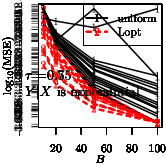
Figure 1: log₁₀(MSE) against number of repeat subsampling $B$. The three columns 1-3 correspond to the three distributions of ${X}$ (normal, $t_{3}$, $t_{2}$), respectively. Rows 1-3 are for $\tau=0.5$ and rows 4-6 are for $\tau=0.75$. Rows 1 and 4, 2 and 5, and 3 and 6 are for cases when $Y$ follows normal, exponential, and $t_{1}$ distributions, respectively.

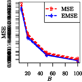
Figure 2: Empirical MSE (MSE) and estimated MSE (EMSE) against number of repeat subsampling $B$ when $\tau=0.75$. The three columns 1-3 correspond to the three distributions of ${X}$ (normal, $t_{3}$, $t_{2}$), respectively. The three rows 1-3 correspond to the three conditional distributions of $Y$ (normal, exponential, $t_{1}$), respectively.

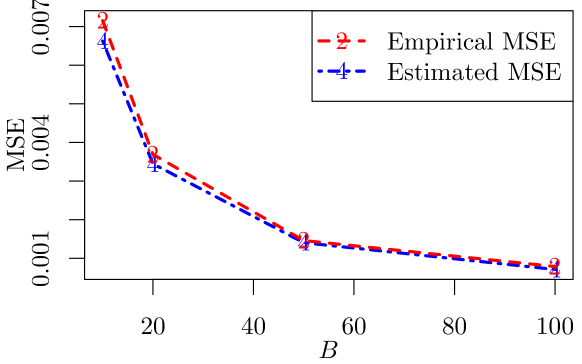
Figure 3: Empirical MSE and estimated MSE against number of repeat subsampling $B$ for the gas sensor data set. The MSE for the full data based on 100 iterations of bootstrapping is $1.95\times 10^{-5}$.

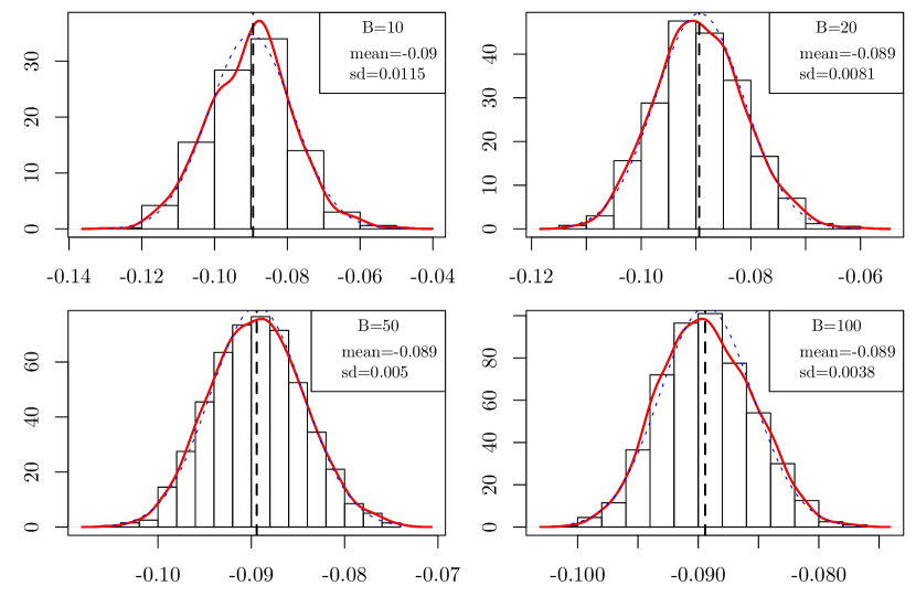
Figure 4: Histograms for $\breve{\beta}_{I,14}^{(s)}$s with different values of $B$. The vertical dashed line corresponding to the value calculated from the full data estimate $\widehat{{\beta}}_{14}$. The red solid curve is the kernel density estimate and the blue dashed curve is the normal density curve with the same mean and standard deviation of $\breve{\beta}_{I,14}^{(s)}s$.

Supplementary material for
Optimal subsampling for quantile regression in big data
by HaiYing Wang and Yanyuan Ma

In this supplementary material, we prove all the theorems in the main paper and provide additional numerical results.

S.1 Proofs of theorems

S.1-1 Proof of Theorem 1

Define

$$Z_{n}^{*}(\lambda)=\sum_{i=1}^{n}\frac{\rho_{\tau}(\varepsilon_{i}^{*}-v_{i}^{*})-\rho_{\tau}(\varepsilon_{i}^{*})}{N\pi_{i}^{*}},$$

where $v_{i}^{*}=\lambda^{\rm T}{x}_{i}^{*}/\sqrt{n}$ and $\varepsilon_{i}^{*}=y_{i}^{*}-{\beta}_{t}^{\rm T}{x}_{i}^{*}$. As a function of $\lambda$, $Z_{n}^{*}(\lambda)$ is convex and minimized by $\sqrt{n}(\widetilde{\beta}-{\beta}_{t})$. Thus we can focus on $Z_{n}^{*}(\lambda)$ when assessing the properties of $\sqrt{n}(\widetilde{\beta}-{\beta}_{t})$.

From the following identity

$$\rho_{\tau}(u-v)-\rho_{\tau}(u)=-v\psi_{\tau}(u)+\int_{0}^{v}\{I(u\leq s)-I(u\leq 0)\}\mathrm{d}s,$$

where $\psi_{\tau}(u)=\tau-I(u<0)$, we have

$$Z_{n}^{*}(\lambda) = \sum_{i=1}^{n}\frac{-v_{i}^{*}\psi_{\tau}(\varepsilon_{i}^{*})+\int_{0}^{v_{i}^{*}}\{I(\varepsilon_{i}^{*}\leq s)-I(\varepsilon_{i}^{*}\leq 0)\}\mathrm{d}s}{N\pi_{i}^{*}}{}$$ (S.1)

$$= \frac{1}{\sqrt{n}}\sum_{i=1}^{n}\frac{-\lambda^{\rm T}{x}_{i}^{*}\{\tau-I(\varepsilon_{i}^{*}<0)\}}{N\pi_{i}^{*}}+\sum_{i=1}^{n}\frac{\int_{0}^{v_{i}^{*}}\{I(\varepsilon_{i}^{*}\leq s)-I(\varepsilon_{i}^{*}\leq 0)\}\mathrm{d}s}{N\pi_{i}^{*}}{}$$

$$= \lambda^{\rm T}W_{n}^{*}+Z_{2n}^{*}.$$

where

$$W_{n}^{*} = -\frac{1}{\sqrt{n}}\sum_{i=1}^{n}\frac{{x}_{i}^{*}\{\tau-I(\varepsilon_{i}^{*}<0)\}}{N\pi_{i}^{*}},$$

$$Z_{2n}^{*} = \sum_{i=1}^{n}\frac{\int_{0}^{v_{i}^{*}}\{I(\varepsilon_{i}^{*}\leq s)-I(\varepsilon_{i}^{*}\leq 0)\}\mathrm{d}s}{N\pi_{i}^{*}}.$$

Denote

$$\eta_{i}^{*} = \frac{-{x}_{i}^{*}\{\tau-I(\varepsilon_{i}^{*}<0)\}}{N\pi_{i}^{*}},$$

so $W_{n}^{*}=n^{-1/2}\sum_{i=1}^{n}\eta_{i}^{*}$. We have

$$\mathbb{E}(\eta_{i}^{*}|\mathcal{F}_{N}) =\sum_{i=1}^{N}\frac{-{x}_{i}\{\tau-I(\varepsilon_{i}<0)\}}{N}=O_{P}(1/\sqrt{N}),$$ (S.2)

$$\mathbb{V}(\eta_{i}^{*}|\mathcal{F}_{N}) =\sum_{i=1}^{N}\frac{\{\tau-I(\varepsilon_{i}<0)\}^{2}{x}_{i}{x}_{i}^{\rm T}}{N^{2}\pi_{i}}-\left[\sum_{i=1}^{N}\frac{-{x}_{i}\{\tau-I(\varepsilon_{i}<0)\}}{N}\right]^{2}={V}_{\pi}-o_{P}(1),$$ (S.3)

where $\varepsilon_{i}=y_{i}-{\beta}_{t}^{\rm T}{x}_{i}$. In (S.2), $\mathbb{E}(\eta_{i}^{*}|\mathcal{F}_{N})$ is $O_{P}(N^{-1/2})$ because for each element of $\eta_{i}^{*}$, say $\eta_{i,j}^{*}$,

$$\mathbb{E}\{\mathbb{E}(\eta_{i,j}^{*}|\mathcal{F}_{N})\} =0$$

$$\mathbb{V}\{\mathbb{E}(\eta_{i,j}^{*}|\mathcal{F}_{N})\} =\frac{1}{N^{2}}\sum_{i=1}^{N}\mathbb{V}\{\tau-I(\varepsilon_{i}<0)\}x_{i,j}^{2}\leq\frac{1}{N^{2}}\sum_{i=1}^{N}\|{x}_{i}\|^{2},$$

and Chebyshev’s inequality indicates that $\mathbb{E}(\eta_{i,j}^{*}|\mathcal{F}_{N})=O_{P}(N^{-1/2})$.

We now check Lindeberg’s conditions (Theorem 2.27 of van der Vaart, 1998) under the conditional distribution given $\mathcal{F}_{N}$. Specifically, we want to show that for every $\epsilon>0$,

$$\sum_{i=1}^{n}\mathbb{E}\{\|n^{-1/2}\eta_{i}^{*}\|^{2}I(\|\eta_{i}^{*}\|>\sqrt{n}\epsilon)\big{|}\mathcal{F}_{N}\}{}$$

$$=\sum_{i=1}^{n}\mathbb{E}\Bigg{\{}\bigg{\|}\frac{-{x}_{i}^{*}\{\tau-I(\varepsilon_{i}^{*}<0)\}}{\sqrt{n}N\pi_{i}^{*}}\bigg{\|}^{2}I\bigg{(}\bigg{\|}\frac{-{x}_{i}^{*}\{\tau-I(\varepsilon_{i}^{*}<0)\}}{\sqrt{n}N\epsilon\pi_{i}^{*}}\bigg{\|}>1\bigg{)}\bigg{|}\mathcal{F}_{N}\Bigg{\}}{}$$

$$=\sum_{i=1}^{N}\frac{\|{x}_{i}\|^{2}\{\tau-I(\varepsilon_{i}<0)\}^{2}}{N^{2}\pi_{i}}I\bigg{(}\frac{\|{x}_{i}\||\tau-I(\varepsilon_{i}<0)|}{\sqrt{n}N\epsilon\pi_{i}}>1\bigg{)}{}$$

$$\leq\sum_{i=1}^{N}\frac{\|{x}_{i}\|^{2}}{N^{2}\pi_{i}}I\bigg{(}\frac{\|{x}_{i}\|}{\sqrt{n}N\epsilon\pi_{i}}>1\bigg{)}$$ (S.4)

goes to zero in probability. If condition (8) holds, then the right hand side of (S.4) satisfies that

$$\sum_{i=1}^{N}\frac{\|{x}_{i}\|^{2}}{N^{2}\pi_{i}}I\bigg{(}\frac{\|{x}_{i}\|}{\sqrt{n}N\epsilon\pi_{i}}>1\bigg{)} \leq \sum_{i=1}^{N}\frac{\|{x}_{i}\|^{2}}{N^{2}\pi_{i}}I\bigg{(}\max_{1\leq i\leq N}\frac{\|{x}_{i}\|}{\pi_{i}}>\sqrt{n}N\epsilon\bigg{)}{}$$

$$= I\bigg{(}\max_{1\leq i\leq N}\frac{\|{x}_{i}\|}{\pi_{i}}>\sqrt{n}N\epsilon\bigg{)}\sum_{i=1}^{N}\frac{\|{x}_{i}\|^{2}}{N^{2}\pi_{i}}=o_{P}(1).{}$$

Thus, combining (S.3) and Assumption 2 (b), if (8) holds, Lindeberg’s conditions hold in probability.

Given $\mathcal{F}_{N}$, $\eta_{i}^{*}$, $i=1,...,n$, are i.i.d with mean $\mathbb{E}(\eta_{i}^{*}|\mathcal{F}_{N})$ and variance $\mathbb{V}(\eta_{i}^{*}|\mathcal{F}_{N})$. Thus, conditional on $\mathcal{F}_{N}$, when $n,N\to\infty$, with probability approaching one,

$$\{\mathbb{V}(\eta_{i}^{*}|\mathcal{F}_{N})\}^{-1/2}\{W_{n}^{*}-\sqrt{n}\mathbb{E}(\eta_{i}^{*}|\mathcal{F}_{N})\}\longrightarrow\mathbb{N}({0},{I}),$$

in distribution, which implies that

$$\{\mathbb{V}(\eta_{i}^{*}|\mathcal{F}_{N})\}^{-1/2}W_{n}^{*}\longrightarrow\mathbb{N}({0},{I}),$$ (S.5)

in distribution because $\sqrt{n}\mathbb{E}(\eta_{i}^{*}|\mathcal{F}_{N})\}=O_{P}(n^{1/2}N^{-1/2})=o_{P}(1)$.

For $Z_{2n}^{*}$ in (S.1), denote $Z_{2ni}^{*}=\int_{0}^{v_{i}^{*}}\{I(\varepsilon_{i}^{*}\leq s)-I(\varepsilon_{i}^{*}\leq 0)\}\mathrm{d}s$, and

$$\mathbb{E}(Z_{2ni}^{*})=\int_{0}^{v_{i}^{*}}\{F_{\varepsilon\mid{X}}(s,{x}_{i}^{*})-F_{\varepsilon\mid{X}}(0,{x}_{i}^{*})\}\mathrm{d}s.$$

The conditional expectation of $Z_{2n}^{*}$, $\mathbb{E}(Z_{2n}^{*}|\mathcal{F}_{N})$, equals

$$\mathbb{E}\left(\sum_{i=1}^{n}\frac{Z_{2ni}^{*}}{N\pi_{i}^{*}}\bigg{|}\mathcal{F}_{N}\right)=\frac{n}{N}\sum_{i=1}^{N}Z_{2ni}=\frac{n}{N}\sum_{i=1}^{N}\mathbb{E}(Z_{2ni})+\frac{n}{N}\sum_{i=1}^{N}\{Z_{2ni}-\mathbb{E}(Z_{2ni})\},$$ (S.6)

where $Z_{2ni}=\int_{0}^{v_{i}}\{I(\varepsilon_{i}\leq s)-I(\varepsilon_{i}\leq 0)\}\mathrm{d}s$, and $\mathbb{E}(Z_{2ni})=\int_{0}^{v_{i}}\{F_{\varepsilon\mid{X}}(s,{x}_{i})-F_{\varepsilon\mid{X}}(0,{x}_{i})\}\mathrm{d}s$. For the first term on the right hand side of (S.6), following an approach similar to that in Section 4.2 of Koenker (2005) under the conditions in Assumption 1, we have

$$\frac{n}{N}\sum_{i=1}^{N}\mathbb{E}(Z_{2ni})= \frac{n}{N}\sum_{i=1}^{N}\int_{0}^{v_{i}}\{F_{\varepsilon\mid{X}}(s,{x}_{i})-F_{\varepsilon\mid{X}}(0,{x}_{i})\}\mathrm{d}s{}$$

$$= \frac{\sqrt{n}}{N}\sum_{i=1}^{N}\int_{0}^{\lambda^{\rm T}{x}_{i}}\{F_{\varepsilon\mid{X}}(t/{\sqrt{n}},{x}_{i})-F_{\varepsilon\mid{X}}(0,{x}_{i})\}\mathrm{d}t{}$$

$$= \frac{1}{N}\sum_{i=1}^{N}\int_{0}^{\lambda^{\rm T}{x}_{i}}f_{\varepsilon\mid{X}}(0,{x}_{i})t\mathrm{d}t+o(1){}$$

$$= \frac{1}{2N}\sum_{i=1}^{N}(\lambda^{\rm T}{x}_{i})^{2}f_{\varepsilon\mid{X}}(0,{x}_{i})+o(1){}$$

$$= \frac{1}{2}\lambda^{\rm T}D_{N}\lambda+o(1)=\frac{1}{2}\lambda^{\rm T}D\lambda+o(1).$$ (S.7)

The second term in (S.6) has mean 0 and variance

$$\mathbb{V}\left\{n\sum_{i=1}^{N}\frac{Z_{2ni}-\mathbb{E}(Z_{2ni})}{N}\right\} \leq\frac{n^{2}}{N^{2}}\sum_{i=1}^{N}\mathbb{E}(Z_{2ni}^{2}){}$$

$$\leq\frac{\max_{1\leq i\leq N}\|{x}_{i}\|}{\sqrt{N}}\times\frac{2\|\lambda\|\sqrt{n}}{\sqrt{N}}\times\frac{n}{N}\sum_{i=1}^{N}\mathbb{E}(Z_{2ni})$$ (S.8)

which, in view of (S.7), converges to 0 if condition (5) holds and $n/N$ does not go to infinity. Here, the second inequality in (S.8) is from the facts that $Z_{2ni}$ is nonnegative and

$$Z_{2ni}\leq\left|\int_{0}^{\frac{\lambda^{\rm T}{x}_{i}}{\sqrt{n}}}|\{I(\varepsilon_{i}\leq s)-I(\varepsilon_{i}\leq 0)\}|\mathrm{d}s\right|\leq\frac{2|\lambda^{\rm T}{x}_{i}|}{\sqrt{n}}.$$

From (S.6), (S.7), and (S.8),

$$\mathbb{E}\left\{\sum_{i=1}^{n}\frac{Z_{2ni}^{*}}{N\pi_{i}^{*}}\bigg{|}\mathcal{F}_{N}\right\}=\frac{n}{N}\sum_{i=1}^{N}Z_{2ni}=\frac{1}{2}\lambda^{\rm T}D_{N}\lambda+o_{P}(1)$$ (S.9)

based on Chebyshev’s inequality.

Now we exam the conditional variance of $Z_{2n}^{*}$. Nothing that conditional on ${\cal F}_{N}$, $Z_{2ni}^{*}$’s are independent and identically distributed, we have

$$\mathbb{V}\left\{\sum_{i=1}^{n}\frac{Z_{2ni}^{*}}{N\pi_{i}^{*}}\bigg{|}\mathcal{F}_{N}\right\}\leq\frac{n}{N^{2}}\mathbb{E}\left\{\frac{(Z_{2ni}^{*})^{2}}{(\pi_{i}^{*})^{2}}\right\}=\frac{n}{N^{2}}\sum_{i=1}^{N}\frac{Z_{2ni}^{2}}{\pi_{i}}{}$$

$$\leq\frac{2\sqrt{n}\|\lambda\|}{N^{2}}\sum_{i=1}^{N}\frac{Z_{2ni}\|{x}_{i}\|}{\pi_{i}}\leq\max_{1\leq i\leq N}\frac{\|{x}_{i}\|}{\pi_{i}}\times\frac{2\sqrt{n}\|\lambda\|}{N^{2}}\sum_{i=1}^{N}Z_{2ni}{}$$

$$=\max_{1\leq i\leq N}\frac{\|{x}_{i}\|}{\pi_{i}}\times\frac{2\|\lambda\|}{\sqrt{n}N}\times\frac{n}{N}\sum_{i=1}^{N}Z_{2ni}.$$ (S.10)

From (S.7), (S.10), and condition (8), we have

$$\mathbb{V}\left\{\sum_{i=1}^{n}\frac{Z_{2ni}^{*}}{N\pi_{i}^{*}}\bigg{|}\mathcal{F}_{N}\right\}=o_{P}(1).$$ (S.11)

From (S.9), (S.11), and Chebyshev’s inequality,

$$\sum_{i=1}^{n}\frac{Z_{2ni}^{*}}{N\pi_{i}^{*}}-\frac{1}{2}\lambda^{\rm T}D_{N}\lambda=o_{P|\mathcal{F}_{N}}(1).$$ (S.12)

Here $a=o_{P|\mathcal{F}_{N}}(1)$ means $a$ converges to zero in conditional probability given $\mathcal{F}_{N}$ in probability, namely, for any $\delta>0$, $\Pr(|a|>\delta|\mathcal{F}_{N})\rightarrow 0$ in probability. Note that $\Pr(|a|>\delta|\mathcal{F}_{N})\leq 1$, thus it converges to 0 in probability if and only if $\Pr(|a|>\delta)=\mathbb{E}\{\Pr(|a|>\delta|\mathcal{F}_{N})\}\rightarrow 0$. Therefore, $a=o_{P|\mathcal{F}_{N}}(1)$ is equivalent to $a=o_{P}(1)$, and we will use the notation of $o_{P}$ only.

From (S.1) and (S.12), we have

$$Z_{n}^{*}(\lambda)=\lambda^{\rm T}W_{n}^{*}+\frac{1}{2}\lambda^{\rm T}D_{N}\lambda+o_{P}(1).$$

Since $Z_{n}^{*}(\lambda)$ is convex, from the corollary in page 2 of Hjort and Pollard (2011), its minimizer, $\sqrt{n}(\widetilde{\beta}-{\beta}_{t})$, satisfies that

$$\sqrt{n}(\widetilde{\beta}-{\beta}_{t})=-D_{N}^{-1}W_{n}^{*}+o_{P}(1),$$

Thus, we have

$$(D_{N}^{-1}{V}_{\pi}D_{N}^{-1})^{-1/2}\sqrt{n}(\widetilde{\beta}-{\beta}_{t})=-(D_{N}^{-1}{V}_{\pi}D_{N}^{-1})^{-1/2}D_{N}^{-1}W_{n}^{*}+o_{P}(1).$$

Combining the the fact that $(D_{N}^{-1}{V}_{\pi}D_{N}^{-1})^{-1/2}D_{N}^{-1}{V}_{\pi}D_{N}^{-1}(D_{N}^{-1}{V}_{\pi}D_{N}^{-1})^{-1/2}={I}$, the results in (S.3) and (S.5), and Slutsky’s Theorem, we have that $(D_{N}^{-1}{V}_{\pi}D_{N}^{-1})^{-1/2}\sqrt{n}(\widetilde{\beta}-{\beta}_{t})$ converges to $\mathbb{N}({0},{I})$ in conditional distribution given $\mathcal{F}_{N}$ in probability. This means that for any ${x}$

$$\Pr\{(D_{N}^{-1}{V}_{\pi}D_{N}^{-1})^{-1/2}\sqrt{n}(\widetilde{\beta}-{\beta}_{t})\leq{x}|\mathcal{F}_{N}\}\rightarrow\Phi({x}),$$ (S.13)

in probability, where $\Phi({x})$ is the cumulative distribution function of the standard multivariate normal distribution. Note that the conditional probability in (S.13) is a bounded random variable, thus convergence in probability to a constant implies convergence in the mean. Therefore, the unconditional probability

$$\Pr\{(D_{N}^{-1}{V}_{\pi}D_{N}^{-1})^{-1/2}\sqrt{n}(\widetilde{\beta}-{\beta}_{t})\leq{x}\}$$

$$= \mathbb{E}[\Pr\{(D_{N}^{-1}{V}_{\pi}D_{N}^{-1})^{-1/2}\sqrt{n}(\widetilde{\beta}-{\beta}_{t})\leq{x}|\mathcal{F}_{N}\}]\rightarrow\Phi({x}).$$

This finishes the proof of Theorem 1.

S.1-2 Proof of Theorem 2

Note that

$$\mathrm{tr}({V}_{\pi}) = \mathrm{tr}\left[\sum_{i=1}^{N}\frac{\{\tau-I(\varepsilon_{i}<0)\}^{2}{x}_{i}{x}_{i}^{\rm T}}{N^{2}\pi_{i}}\right]$$

$$= \frac{1}{N^{2}}\sum_{i=1}^{N}\mathrm{tr}\left[\frac{\{\tau-I(\varepsilon_{i}<0)\}^{2}{x}_{i}{x}_{i}^{\rm T}}{\pi_{i}}\right]$$

$$= \frac{1}{N^{2}}\sum_{i=1}^{N}\frac{\{\tau-I(\varepsilon_{i}<0)\}^{2}\|{x}_{i}\|^{2}}{\pi_{i}}$$

$$= \frac{1}{N^{2}}\left(\sum_{i=1}^{N}\pi_{i}\right)\left(\sum_{i=1}^{N}\frac{\{\tau-I(\varepsilon_{i}<0)\}^{2}\|{x}_{i}\|^{2}}{\pi_{i}}\right)$$

$$\geq \frac{1}{N^{2}}\left\{\sum_{i=1}^{N}|\tau-I(\varepsilon_{i}<0)|\|{x}_{i}\|\right\}^{2},$$

where the last step is from the Cauchy-Schwarz inequality and the equality in it holds if and only if when $\pi_{i}\propto|\tau-I(\varepsilon_{i}<0)|\|{x}_{i}\|$.

S.1-3 Proof of Theorem 3

Note that

$$\mathrm{tr}(D_{N}^{-1}{V}_{\pi}D_{N}^{-1}) = \mathrm{tr}\left[D_{N}^{-1}\sum_{i=1}^{N}\frac{\{\tau-I(\varepsilon_{i}<0)\}^{2}{x}_{i}{x}_{i}^{\rm T}}{N^{2}\pi_{i}}D_{N}^{-1}\right]$$

$$= \frac{1}{N^{2}}\sum_{i=1}^{N}\mathrm{tr}\left[\frac{\{\tau-I(\varepsilon_{i}<0)\}^{2}D_{N}^{-1}{x}_{i}{x}_{i}^{\rm T}D_{N}^{-1}}{\pi_{i}}\right]$$

$$= \frac{1}{N^{2}}\sum_{i=1}^{N}\frac{\{\tau-I(\varepsilon_{i}<0)\}^{2}\|D_{N}^{-1}{x}_{i}\|^{2}}{\pi_{i}}$$

$$= \frac{1}{N^{2}}\left(\sum_{i=1}^{N}\pi_{i}\right)\left(\sum_{i=1}^{N}\frac{\{\tau-I(\varepsilon_{i}<0)\}^{2}\|D_{N}^{-1}{x}_{i}\|^{2}}{\pi_{i}}\right)$$

$$\geq \frac{1}{N^{2}}\left\{\sum_{i=1}^{N}|\tau-I(\varepsilon_{i}<0)|\|D_{N}^{-1}{x}_{i}\|\right\}^{2},$$

where the last step is from the Cauchy-Schwarz inequality and the equality in it holds if and only if when $\pi_{i}\propto|\tau-I(\varepsilon_{i}<0)|\|D_{N}^{-1}{x}_{i}\|$.

S.1-4 Proof of Theorem 4

Recall the notations $v_{i}^{*}=\lambda^{\rm T}{x}_{i}^{*}/\sqrt{n}$, $\varepsilon_{i}^{*}=y_{i}^{*}-{\beta}_{t}^{\rm T}{x}_{i}^{*}$, and $\psi_{\tau}(u)=\tau-I(u<0)$. Let

$$\breve{Z}_{n}(\lambda)= \sum_{i=1}^{n}\frac{\rho_{\tau}(\varepsilon_{i}^{*}-v_{i}^{*})-\rho_{\tau}(\varepsilon_{i}^{*})}{N\pi_{i}^{*\widetilde{\beta}_{0}}},{}$$

$$= \sum_{i=1}^{n}\frac{-v_{i}^{*}\psi_{\tau}(\varepsilon_{i}^{*})+\int_{0}^{v_{i}^{*}}\{I(\varepsilon_{i}^{*}\leq s)-I(\varepsilon_{i}^{*}\leq 0)\}\mathrm{d}s}{N\pi_{i}^{*\widetilde{\beta}_{0}}},{}$$

$$= \frac{1}{\sqrt{n}}\sum_{i=1}^{n}\frac{-\lambda^{\rm T}{x}_{i}^{*}\{\tau-I(\varepsilon_{i}^{*}<0)\}}{N\pi_{i}^{*\widetilde{\beta}_{0}}}+\sum_{i=1}^{n}\frac{\int_{0}^{v_{i}^{*}}\{I(\varepsilon_{i}^{*}\leq s)-I(\varepsilon_{i}^{*}\leq 0)\}\mathrm{d}s}{N\pi_{i}^{*\widetilde{\beta}_{0}}},{}$$

$$\equiv \lambda^{\rm T}\breve{W}_{n}^{*}+\breve{Z}_{2n}^{*}.$$ (S.14)

Denote

$$\breve{\eta}_{i}^{*}=\frac{-{x}_{i}^{*}\{\tau-I(\varepsilon_{i}^{*}<0)\}}{N\pi_{i}^{*\widetilde{\beta}_{0}}}.$$

We have

$$\mathbb{E}(\breve{\eta}_{i}^{*}|\mathcal{F}_{N},\widetilde{\beta}_{0})= \sum_{i=1}^{N}\frac{-{x}_{i}\{\tau-I(\varepsilon_{i}<0)\}}{N}=O_{P}(N^{-1/2}){}$$

$$\mathbb{V}(\breve{\eta}_{i}^{*}|\mathcal{F}_{N},\widetilde{\beta}_{0})= \sum_{i=1}^{N}\frac{\{\tau-I(\varepsilon_{i}<0)\}^{2}{x}_{i}{x}_{i}^{\rm T}}{N^{2}\pi_{i}^{\widetilde{\beta}_{0}}}-o_{P}(1)$$ (S.15)

For $\pi_{i}^{{\mathrm{Aopt}}}$, $\pi_{i}^{\widetilde{\beta}_{0}}=\pi_{i}^{{\mathrm{Aopt}}}(\widetilde{\beta}_{0})$, and we have

$$\sum_{i=1}^{N}\frac{\{\tau-I(\varepsilon_{i}<0)\}^{2}{x}_{i}{x}_{i}^{\rm T}}{N^{2}\pi_{i}^{{\mathrm{Aopt}}}(\widetilde{\beta}_{0})}{}$$

$$= \frac{1}{N}\sum_{i=1}^{N}\frac{\{\tau-I(\varepsilon_{i}<0)\}^{2}{x}_{i}{x}_{i}^{\rm T}}{|\tau-I(\varepsilon_{i}^{\widetilde{\beta}_{0}}<0)|\|\widetilde{D}_{N}^{-1}{x}_{i}\|}\times\frac{1}{N}\sum_{i=1}^{N}|\tau-I(\varepsilon_{i}^{\widetilde{\beta}_{0}}<0)|\|\widetilde{D}_{N}^{-1}{x}_{i}\|\equiv\widetilde{\Delta}_{1}\times\widetilde{\Delta}_{2}.$$ (S.16)

Now we show that $\widetilde{\Delta}_{1}-\Delta_{1}=o_{P}(1)$ and $\widetilde{\Delta}_{2}-\Delta_{2}=o_{P}(1)$, where $\Delta_{1}$ and $\Delta_{2}$ have the same expression of $\widetilde{\Delta}_{1}$ and $\widetilde{\Delta}_{2}$, respectively, except that $\varepsilon_{i}^{\widetilde{\beta}_{0}}=y_{i}-\widetilde{\beta}_{0}^{\rm T}{x}_{i}$ and $\widetilde{D}_{N}$ are replaced by $\varepsilon_{i}$ and $D_{N}$, respectively. Denote $\tau_{m}=\min(\tau,1-\tau)$. For the $j_{1},j_{2}$th element of $\widetilde{\Delta}_{1}-\Delta_{1}$, $j_{1},j_{2}=1,...,p$,

$$|\widetilde{\Delta}_{1}-\Delta_{1}|_{j_{1},j_{2}}\leq \frac{1}{N}\sum_{i=1}^{N}\Bigg{|}\frac{\{\tau-I(\varepsilon_{i}<0)\}^{2}\|{x}_{i}\|^{2}}{|\tau-I(\varepsilon_{i}^{\widetilde{\beta}_{0}}<0)|\|{D}_{N}^{-1}{x}_{i}\|}-\frac{\{\tau-I(\varepsilon_{i}<0)\}^{2}\|{x}_{i}\|^{2}}{|\tau-I(\varepsilon_{i}<0)|\|D_{N}^{-1}{x}_{i}\|}\Bigg{|}{}$$

$$+\frac{1}{N}\sum_{i=1}^{N}\Bigg{|}\frac{\{\tau-I(\varepsilon_{i}<0)\}^{2}\|{x}_{i}\|^{2}}{|\tau-I(\varepsilon_{i}^{\widetilde{\beta}_{0}}<0)|\|\widetilde{D}_{N}^{-1}{x}_{i}\|}-\frac{\{\tau-I(\varepsilon_{i}<0)\}^{2}\|{x}_{i}\|^{2}}{|\tau-I(\varepsilon_{i}^{\widetilde{\beta}_{0}}<0)|\|D_{N}^{-1}{x}_{i}\|}\Bigg{|}$$ (S.17)

$$\leq \frac{1}{N}\sum_{i=1}^{N}\Bigg{|}\frac{|\tau-I(\varepsilon_{i}<0)|\|{x}_{i}\|^{2}}{|\tau-I(\varepsilon_{i}^{\widetilde{\beta}_{0}}<0)|\|D_{N}^{-1}{x}_{i}\|}-\frac{|\tau-I(\varepsilon_{i}^{\widetilde{\beta}_{0}}<0)|\|{x}_{i}\|^{2}}{|\tau-I(\varepsilon_{i}^{\widetilde{\beta}_{0}}<0)|\|D_{N}^{-1}{x}_{i}\|}\Bigg{|}+o_{P}(1){}$$

$$\leq \frac{1}{\tau_{m}N}\sum_{i=1}^{N}\frac{|I(\varepsilon_{i}^{\widetilde{\beta}_{0}}<0)-I(\varepsilon_{i}<0)|\|{x}_{i}\|^{2}}{\|D_{N}^{-1}{x}_{i}\|}+o_{P}(1){}$$

$$\leq \frac{\lambda_{\max}^{D}\{1+o_{P}(1)\}}{\tau_{m}N}\sum_{i=1}^{N}|I(\varepsilon_{i}^{\widetilde{\beta}_{0}}<0)-I(\varepsilon_{i}<0)|\|{x}_{i}\|+o_{P}(1),$$ (S.18)

in which $\lambda_{\max}^{D}$ is the largest eigenvalue of $D$. Here, the term in (S.17) is $o_{P}(1)$ due to the uniform convergence of $\widetilde{f}_{\varepsilon\mid{X}}(0,{x})$; the second last inequality also used $\widetilde{\beta}_{0}-{\beta}_{t}=o_{p}(1)$; and $D_{N}$ can be replaced in the last step by its limit $D$ because of condition (4). For any $\epsilon>0$,

$$\Pr\Bigg{\{}\frac{1}{N}\sum_{i=1}^{N}|I(\varepsilon_{i}^{\widetilde{\beta}_{0}}<0)-I(\varepsilon_{i}<0)|\|{x}_{i}\|>\epsilon\Bigg{\}}{}$$

$$\leq\frac{1}{\epsilon N}\sum_{i=1}^{N}\mathbb{E}\{|I(\varepsilon_{i}^{\widetilde{\beta}_{0}}<0)-I(\varepsilon_{i}<0)|\}\|{x}_{i}\|.$$ (S.19)

Note that for each $i$, $|I(\varepsilon_{i}^{\widetilde{\beta}_{0}}<0)-I(\varepsilon_{i}<0)|$ is bounded and converges in probability to 0, as $n_{0}\rightarrow\infty$ and $n\rightarrow\infty$. Thus, $\mathbb{E}\{|I(\varepsilon_{i}^{\widetilde{\beta}_{0}}<0)-I(\varepsilon_{i}<0)|\}\rightarrow 0$. This indicates that the term in (S.19) converges to 0, which implies that the term in (S.18) converges in probability to 0. Thus, $\widetilde{\Delta}_{1}-\Delta_{1}=o_{P}(1)$. Using a similar approach, it can be shown that $\widetilde{\Delta}_{2}-\Delta_{2}=o_{P}(1)$. These facts, together with (S.15) and (S.16), show that, for $\pi_{i}^{{\mathrm{Aopt}}}$,

$$\mathbb{V}(\breve{\eta}_{i}^{*}|\mathcal{F}_{N},\widetilde{\beta}_{0})= \sum_{i=1}^{N}\frac{\{\tau-I(\varepsilon_{i}<0)\}^{2}{x}_{i}{x}_{i}^{\rm T}}{N^{2}\pi_{i}^{{\mathrm{Aopt}}}}+o_{P}(1).$$ (S.20)

For $\pi_{i}^{{\mathrm{Lopt}}}$, $\pi_{i}^{\widetilde{\beta}_{0}}=\pi_{i}^{{\mathrm{Lopt}}}(\widetilde{\beta}_{0})$, and we have

$$\sum_{i=1}^{N}\frac{\{\tau-I(\varepsilon_{i}<0)\}^{2}{x}_{i}{x}_{i}^{\rm T}}{N^{2}\pi_{i}^{{\mathrm{Lopt}}}(\widetilde{\beta}_{0})}{}$$

$$=\frac{1}{N}\sum_{i=1}^{N}\frac{\{\tau-I(\varepsilon_{i}<0)\}^{2}{x}_{i}{x}_{i}^{\rm T}}{|\tau-I(\varepsilon_{i}^{\widetilde{\beta}_{0}}<0)|\|{x}_{i}\|}\times\frac{1}{N}\sum_{i=1}^{N}|\tau-I(\varepsilon_{i}^{\widetilde{\beta}_{0}}<0)|\|{x}_{i}\|\equiv\widetilde{\Delta}_{3}\times\widetilde{\Delta}_{4}.$$ (S.21)

Now we show that $\widetilde{\Delta}_{3}-\Delta_{3}=o_{P}(1)$ and $\widetilde{\Delta}_{4}-\Delta_{4}=o_{P}(1)$, where $\Delta_{3}$ and $\Delta_{4}$ have the same expression of $\widetilde{\Delta}_{3}$ and $\widetilde{\Delta}_{4}$, respectively, except that $\varepsilon_{i}^{\widetilde{\beta}_{0}}$ is replaced by $\varepsilon_{i}$. Note that the $j_{1},j_{2}$th element of $\widetilde{\Delta}_{3}-\Delta_{3}$ or $\widetilde{\Delta}_{4}-\Delta_{4}$, $j_{1},j_{2}=1,...,p$, is bounded by

$$\frac{1}{\tau_{m}N}\sum_{i=1}^{N}|I(\varepsilon_{i}^{\widetilde{\beta}_{0}}<0)-I(\varepsilon_{i}<0)|\|{x}_{i}\|.$$ (S.22)

Using a similar approach used for the case of $\pi_{i}^{{\mathrm{Aopt}}}$, (S.22) can be shown to be $o_{P}(1)$. Thus, $\widetilde{\Delta}_{3}-\Delta_{3}=o_{P}(1)$ and $\widetilde{\Delta}_{4}-\Delta_{4}=o_{P}(1)$. These facts, together with (S.15), yield that, for $\pi_{i}^{{\mathrm{Lopt}}}$,

$$\mathbb{V}(\breve{\eta}_{i}^{*}|\mathcal{F}_{N},\widetilde{\beta}_{0})= \sum_{i=1}^{N}\frac{\{\tau-I(\varepsilon_{i}<0)\}^{2}{x}_{i}{x}_{i}^{\rm T}}{N^{2}\pi_{i}^{{\mathrm{Lopt}}}}+o_{P}(1).$$ (S.23)

We now check the Lindeberg’s condition given $\mathcal{F}_{N}$ and $\widetilde{\beta}_{0}$.
For every $\epsilon>0$,

$$\sum_{i=1}^{n}\mathbb{E}(\|n^{-1/2}\breve{\eta}_{i}^{*}\|^{2}I(\|\breve{\eta}_{i}^{*}\|>\sqrt{n}\epsilon)\big{|}\mathcal{F}_{N},\widetilde{\beta}_{0}){}$$

$$= \sum_{i=1}^{n}\mathbb{E}\Bigg{[}\bigg{\|}\frac{-{x}_{i}^{*}\{\tau-I(\varepsilon_{i}^{*}<0)\}}{\sqrt{n}N\pi_{i}^{*\widetilde{\beta}_{0}}}\bigg{\|}^{2}I\bigg{(}\bigg{\|}\frac{-{x}_{i}^{*}\{\tau-I(\varepsilon_{i}^{*}<0)\}}{\sqrt{n}N\epsilon\pi_{i}^{*\widetilde{\beta}_{0}}}\bigg{\|}>1\bigg{)}\bigg{|}\mathcal{F}_{N},\widetilde{\beta}_{0}\Bigg{]}{}$$

$$= \sum_{i=1}^{N}\frac{\|{x}_{i}\|^{2}\{\tau-I(\varepsilon_{i}<0)\}^{2}}{N^{2}\pi_{i}^{\widetilde{\beta}_{0}}}I\bigg{(}\frac{\|{x}_{i}\||\tau-I(\varepsilon_{i}<0)|}{\sqrt{n}N\epsilon\pi_{i}^{\widetilde{\beta}_{0}}}>1\bigg{)}{}$$

$$\leq \frac{1}{N^{2}}\sum_{i=1}^{N}\frac{\|{x}_{i}\|^{2}}{\pi_{i}^{\widetilde{\beta}_{0}}}I\bigg{(}\frac{\|{x}_{i}\|}{\sqrt{n}N\epsilon\pi_{i}^{\widetilde{\beta}_{0}}}>1\bigg{)}\leq I\bigg{(}\max_{1\leq i\leq N}\frac{\|{x}_{i}\|}{\sqrt{n}N\epsilon\pi_{i}^{\widetilde{\beta}_{0}}}>1\bigg{)}\frac{1}{N^{2}}\sum_{i=1}^{N}\frac{\|{x}_{i}\|^{2}}{\pi_{i}^{\widetilde{\beta}_{0}}}.$$ (S.24)

Now we show that the term on the right-hand-size of (S.24) is $o_{P}(1)$.

For $\pi_{i}^{{\mathrm{Aopt}}}$,

$$\frac{\|{x}_{i}\|}{\pi_{i}^{\widetilde{\beta}_{0}}}= \frac{\|{x}_{i}\|}{|\tau-I(\varepsilon_{i}^{\widetilde{\beta}_{0}}<0)|\|\widetilde{D}_{N}^{-1}{x}_{i}\|}\sum_{j=1}^{N}|\tau-I(\varepsilon_{j}^{\widetilde{\beta}_{0}}<0)|\|\widetilde{D}_{N}^{-1}{x}_{j}\|$$

$$\leq \frac{N}{\tau_{m}}\frac{\|{x}_{i}\|}{\|\widetilde{D}_{N}^{-1}{x}_{i}\|}\times\frac{1}{N}\sum_{j=1}^{N}\|\widetilde{D}_{N}^{-1}{x}_{j}\|$$

$$\leq \frac{N\lambda_{\max}^{\widetilde{D}_{N}}}{\tau_{m}\lambda_{\min}^{\widetilde{D}_{N}}}\times\frac{\|{x}_{i}\|}{\|{x}_{i}\|}\times\frac{1}{N}\sum_{j=1}^{N}\|{x}_{j}\|\leq\frac{N\lambda_{\max}^{D}\sqrt{\mathrm{tr}(D_{0})}}{\tau_{m}\lambda_{\min}^{D}}\{1+o_{P}(1)\},$$

where the $o_{P}(1)$ does not depend on $i$. Thus,

$$\max_{1\leq i\leq N}\frac{\|{x}_{i}\|}{\pi_{i}^{\widetilde{\beta}_{0}}}\leq\frac{N\lambda_{\max}^{D}\sqrt{\mathrm{tr}(D_{0})}}{\tau_{m}\lambda_{\min}^{D}}\{1+o_{P}(1)\}.$$ (S.25)

From (S.24) and (S.25),

$$\sum_{i=1}^{n}\mathbb{E}(\|n^{-1/2}\breve{\eta}_{i}^{*}\|^{2}I(\|\breve{\eta}_{i}^{*}\|>\sqrt{n}\epsilon)\big{|}\mathcal{F}_{N},\widetilde{\beta}_{0}){}$$

$$\leq \frac{1}{N^{2}}\sum_{i=1}^{N}\frac{\|{x}_{i}\|^{2}}{\pi_{i}^{\widetilde{\beta}_{0}}}I\bigg{(}\max_{1\leq i\leq N}\frac{\|{x}_{i}\|}{\sqrt{n}N\epsilon\pi_{i}^{\widetilde{\beta}_{0}}}>1\bigg{)}{}$$

$$\leq I\bigg{(}\frac{\lambda_{\max}^{D}\sqrt{\mathrm{tr}(D_{0})}}{\sqrt{n}\epsilon\tau_{m}\lambda_{\min}^{D}}\{1+o_{P}(1)\}>1\bigg{)}\frac{1}{N^{2}}\sum_{i=1}^{N}\frac{\|{x}_{i}\|^{2}}{\pi_{i}^{\widetilde{\beta}_{0}}}=o_{P}(1).$$

For $\pi_{i}^{{\mathrm{Lopt}}}$,

$$\frac{\|{x}_{i}\|}{\pi_{i}^{\widetilde{\beta}_{0}}}=\frac{\|{x}_{i}\|}{|\tau-I(\varepsilon_{i}^{\widetilde{\beta}_{0}}<0)|\|{x}_{i}\|}\sum_{j=1}^{N}|\tau-I(\varepsilon_{j}^{\widetilde{\beta}_{0}}<0)|\|{x}_{j}\|\leq\frac{1}{\tau_{m}}\sum_{j=1}^{N}\|{x}_{j}\|.$$ (S.26)

Thus, using an approach similar to that used for the case of $\pi_{i}^{{\mathrm{Aopt}}}$, the right hand side of (S.24) is $o_{P}(1)$.

Given $\mathcal{F}_{N}$ and $\widetilde{\beta}_{0}$, $\breve{\eta}_{i}^{*}$, $i=1,...,n$, are i.i.d with mean $o_{P}(1)$ and variance ${V}_{{\mathrm{opt}}}+o_{P}(1)$, where ${V}_{{\mathrm{opt}}}$ has the expression of ${V}_{{\mathrm{Lopt}}}$ in (14) for $\pi_{i}^{{\mathrm{Lopt}}}$ or ${V}_{{\mathrm{Lopt}}}$ in (15) for $\pi_{i}^{{\mathrm{Aopt}}}$. Note that if $N^{-1}\sum_{i=1}^{N}\|{x}_{i}\|^{-1}{{x}_{i}{x}_{i}^{\rm T}}$ is asymptotically positive definite, then ${V}_{{\mathrm{opt}}}$ is asymptotically positive definite because $|\tau-I(\varepsilon_{i}<0)|$ is bounded away from both 0 and infinity and $D_{N}$ converges to a finite positive definite matrix. Thus, given $\mathcal{F}_{N}$ and $\widetilde{\beta}_{0}$ in probability, as $n_{0}\rightarrow\infty$, $n\rightarrow\infty$, and $N\rightarrow\infty$, if $n/N\rightarrow 0$, then

$${V}_{{\mathrm{opt}}}^{-1/2}\breve{W}_{n}^{*}\longrightarrow\mathbb{N}({0},{I}),$$

in distribution.

Note that $Z_{2ni}^{*}=\int_{0}^{v_{i}^{*}}\{I(\varepsilon_{i}^{*}\leq s)-I(\varepsilon_{i}^{*}\leq 0)\}\mathrm{d}s$ and $\mathbb{E}(Z_{2ni})^{*}=\int_{0}^{v_{i}^{*}}\{F_{i}^{*}(s)-f_{\varepsilon\mid{X}}(0,{x}_{i}^{*})\}\mathrm{d}s$. For the second term in (S.14), i.e. $\breve{Z}_{2n}^{*}$, we have

$$\mathbb{E}(\breve{Z}_{2n}^{*}|\mathcal{F}_{N},\widetilde{\beta}_{0})= \mathbb{E}\left\{\sum_{i=1}^{n}\frac{Z_{2ni}^{*}}{N\pi_{i}^{*\widetilde{\beta}_{0}}}\bigg{|}\mathcal{F}_{N},\widetilde{\beta}_{0}\right\}=\frac{n}{N}\sum_{i=1}^{N}Z_{2ni}=\frac{1}{2}\lambda^{\rm T}D_{N}\lambda+o_{P}(1),$$ (S.27)

where the last equality is from (S.9).

Now we exam its variance, which is

$$\mathbb{V}\left\{\sum_{i=1}^{n}\frac{Z_{2ni}^{*}}{N\pi_{i}^{*\widetilde{\beta}_{0}}}\bigg{|}\mathcal{F}_{N},\widetilde{\beta}_{0}\right\}\leq\frac{n}{N^{2}}\mathbb{E}\left\{\frac{(Z_{2ni}^{*})^{2}}{(\pi_{i}^{*\widetilde{\beta}_{0}})^{2}}\bigg{|}\mathcal{F}_{N},\widetilde{\beta}_{0}\right\}=\frac{n}{N^{2}}\sum_{i=1}^{N}\frac{Z_{2ni}^{2}}{\pi_{i}^{\widetilde{\beta}_{0}}}{}$$

$$\leq \frac{2\sqrt{n}\|\lambda\|}{N^{2}}\sum_{i=1}^{N}\frac{Z_{2ni}\|{x}_{i}\|}{\pi_{i}^{\widetilde{\beta}_{0}}}\leq\max_{1\leq i\leq N}\frac{\|{x}_{i}\|}{\pi_{i}^{\widetilde{\beta}_{0}}}\times\frac{2\sqrt{n}\|\lambda\|}{N^{2}}\sum_{i=1}^{N}Z_{2ni}{}$$

$$= \max_{1\leq i\leq N}\frac{\|{x}_{i}\|}{\pi_{i}^{\widetilde{\beta}_{0}}}\times\frac{2\|\lambda\|}{\sqrt{n}N}\times\frac{n}{N}\sum_{i=1}^{N}Z_{2ni}.$$

Considering (S.25) or (S.26), corresponding to $\pi_{i}^{{\mathrm{Aopt}}}$ or $\pi_{i}^{{\mathrm{Lopt}}}$, respectively, and results in (S.9), we have

$$\mathbb{V}(\breve{Z}_{2n}^{*}|\mathcal{F}_{N},\widetilde{\beta}_{0})=\mathbb{V}\left\{\sum_{i=1}^{n}\frac{Z_{2ni}^{*}}{N\pi_{i}^{*\widetilde{\beta}_{0}}}\bigg{|}\mathcal{F}_{N},\widetilde{\beta}_{0}\right\}=O_{P}(n^{-1/2}).$$ (S.28)

From (S.27), (S.28), and Chebyshev’s inequality,

$$\sum_{i=1}^{n}\frac{Z_{2ni}^{*}}{N\pi_{i}^{*\widetilde{\beta}_{0}}}-\frac{1}{2}\lambda^{\rm T}D_{N}\lambda=o_{P}(1).$$ (S.29)

From (S.14) and (S.29),

$$\breve{Z}_{n}^{*}(\lambda)=\lambda^{\rm T}\breve{W}_{n}^{*}+\frac{1}{2}\lambda^{\rm T}D_{N}\lambda+o_{P}(1).$$ (S.30)

Since $\breve{Z}_{n}^{*}(\lambda)$ is convex, from the corollary in page 2 of Hjort and Pollard (2011), its minimizer, $\sqrt{n}(\breve{\beta}-{\beta}_{t})$, satisfies that

$$\sqrt{n}(\breve{\beta}_{{\mathrm{opt}}}-{\beta}_{t})=-D_{N}^{-1}\breve{W}_{n}^{*}+o_{P}(1),$$

where $\breve{\beta}_{{\mathrm{opt}}}=\breve{\beta}_{{\mathrm{Lopt}}}$ for $\pi_{i}^{{\mathrm{Lopt}}}$ and $\breve{\beta}_{{\mathrm{opt}}}=\breve{\beta}_{{\mathrm{Aopt}}}$ for $\pi_{i}^{{\mathrm{Aopt}}}$. Thus, we have

$$(D_{N}^{-1}{V}_{{\mathrm{opt}}}D_{N}^{-1})^{-1/2}\sqrt{n}(\breve{\beta}_{{\mathrm{opt}}}-{\beta}_{t})=-(D_{N}^{-1}{V}_{{\mathrm{opt}}}D_{N}^{-1})^{-1/2}D_{N}^{-1}\breve{W}_{n}^{*}+o_{P}(1),$$

which implies that $(D_{N}^{-1}{V}_{{\mathrm{opt}}}D_{N}^{-1})^{-1/2}\sqrt{n}(\breve{\beta}_{{\mathrm{opt}}}-{\beta}_{t})$ converges to $\mathbb{N}({0},{I})$ in conditional distribution given $\mathcal{F}_{N}$ and $\widetilde{\beta}_{0}$ in probability, meaning that for any ${x}$

$$\Pr\{(D_{N}^{-1}{V}_{{\mathrm{opt}}}D_{N}^{-1})^{-1/2}\sqrt{n}(\breve{\beta}_{{\mathrm{opt}}}-{\beta}_{t})\leq{x}|\mathcal{F}_{N},\widetilde{\beta}_{0}\}\rightarrow\Phi({x}),$$

in probability. Since the conditional probability is a bounded random variable, convergence in probability to a constant implies convergence in the mean. Therefore, the unconditional probability converges and this finishes the proof of Theorem 4.

S.2 Additional numerical results

S.2-1 Multiple quantile levels, including some extreme levels

In this section, we carry out simulations to assess the performance of the proposed method in comparison with the full data estimator at multiple quantile levels, including some extreme levels. Specifically, we let $\tau=0.01,0.02,0.05,0.1,0.3,0.5,0.7,0.9,0.95,0.98$ and $0.99$. We set the full data sample size $N=10^{6}$; set the pilot subsample size $n_{0}=10^{3}$; and set the subsample size $n=10^{3},2\times 10^{3},3\times 10^{3}$, and $5\times 10^{3}$ with $B=10$ so the total subsample sizes are $n=10^{4},2\times 10^{4},3\times 10^{4}$, and $5\times 10^{4}$, respectively. The same model setup as presented in Section 5 of the main paper is used here.

To evaluate the relative efficiency of the proposed method compared with the full data estimator, the first plot in Figure S.1 presents the relative performance ${\text{MSE}_{\text{full}}}/{\text{MSE}_{\text{Lopt}}}$. Clearly, as the subsample size $n$ increases, the estimation efficiency of the proposed method gets higher. It is also seen that all relative MSEs are smaller than one, meaning that the performance in terms of MSE of the full data estimator is always better than that of the subsample estimator, regardless of the quantile level. This is because the subsample based analysis provides estimators at $\sqrt{nB}$-rate while the full data based analysis generates estimators at $\sqrt{N}$-rate.

To eliminate the effect from different sample sizes, we also reported the sample size adjusted MSE ratio, $(N\ \text{MSE}_{\text{full}})/(nB\ \text{MSE}_{\text{Lopt}})$, in the second plot of Figure S.1 for more informative comparisons. This ratio can be interpreted as a measure to compare the per-observation efficiency between the proposed method and the full data analysis. It is seen that most of the ratios are larger than one, expect for extreme quantile levels such as $\tau=0.01$ and $\tau=0.99$. This indicates that smaller sample size is hardly enough to provide useful information for extreme quantile levels. As soon as the sample size is sufficient to perform meaningful analysis, the adjusted MSE improves very fast. Interestingly, as soon as the sample size is reasonably large for the corresponding quantile estimation, the subsample analysis tends to outperform the full data analysis in terms of adjusted MSE. This is because the optimized subsampling probabilities select better subsamples for which the observations are on average more informative than the observations in the full data.

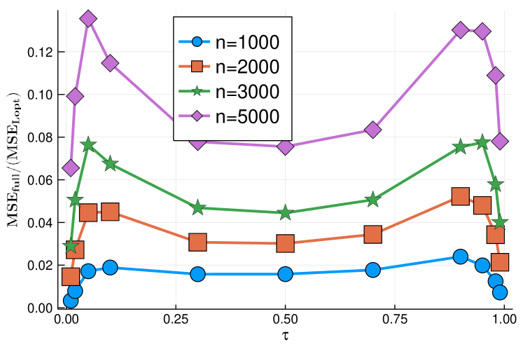
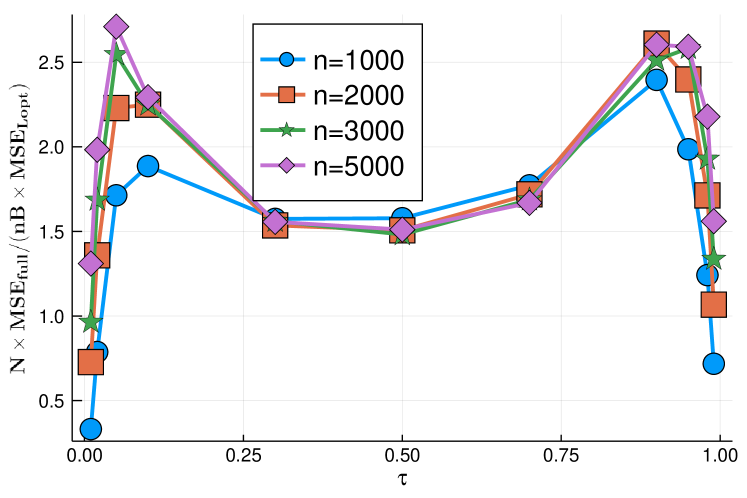
Figure S.1: Ratio of MSE for the subsample estimator to that of the full data estimator against $\tau$. Here $B=10$ and $n$ are set to four different values, ${X}\sim t_{3}$, and the conditional distributions of $Y$ is exponential.

S.2-2 Sensitivity with respect to the subsample size

In this section, we investigate the sensitivity issue of the proposed method with respect to subsample size $n$. We consider two scenarios: one with relatively large subsample sizes and one with small subsample sizes.

Figure S.2 provides the sensitivity of bias and variance to the subsample size $n$ when $n$ is relatively large. From Theorem 4, we know that when the subsample size is large, the variance decreases at the $n^{-1}$ rate, so we plot $n\times$variance against $n$, where the variance is the sum of variances for all regression coefficients. The exact convergence of the bias is unknown so we plot the sum of the absolute biases for all regression coefficients. From Figure S.2, we see that the bias has a clear decreasing trend when sample size increases, and the variance is clearly decreasing at the $n^{-1}$ rate for most quantile levels because the curves are relatively flat. For extreme quantile levels such as $\tau=0.01,0.02$, and $0.99$, there is a decreasing pattern for $n\times$variance, meaning that a larger sample size is required for the asymptotic distribution to be precise. Figure S.3 provides similar sensitivity analysis results when $n$ is small. The general trend is the same, in that both the bias and the variance decrease when $n$ increases. Interestingly, even though the sample sizes are small, at most quantile levels, we can still see the decreasing of the variance at the $n^{-1}$ rate.

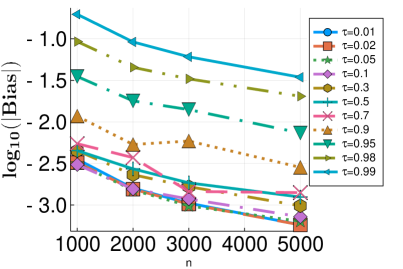
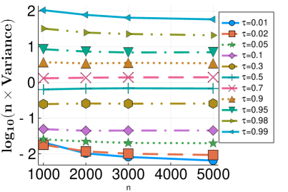
Figure S.2: Absolute bias and $n\times$variance against relatively large values of $n$ with $B=10$ and different quantile levels. Logarithm is taken for better presentation. Here, ${X}\sim t_{3}$ and the conditional distributions of $Y$ is exponential.

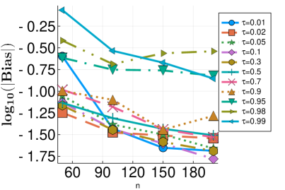
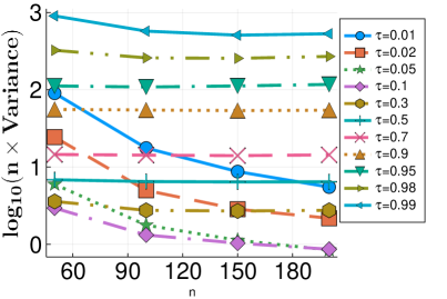
Figure S.3: Absolute bias and $n\times$variance against small values of $n$ with $B=1$ and different quantile levels. Logarithm is taken for better presentation. Here, ${X}\sim t_{3}$ and the conditional distributions of $Y$ is exponential.

S.2-3 Universal subsampling probabilities for multiple quantile levels.

In this section, we provide additional numerical results to evaluate the performance of the sub-optimal universal sampling probabilities $\pi_{i}^{U}$’s derived at the end of Section 4 in the main paper. We use the same model setup and sample size configurations as presented in Section S.2-1. Figure S.4 presents the MSE for subsampling estimator based on both $\pi_{i}^{{\mathrm{Lopt}}}$ and $\pi_{i}^{U}$. We see that although $\pi_{i}^{U}$ may not be as efficient as $\pi_{i}^{{\mathrm{Lopt}}}$ for most quantile levels, the efficiency loss is not severe.

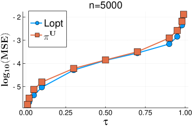
Figure S.4: log₁₀(MSE) against against quantile level $\tau$ for different subsample size $n$ and a fixed $B=10$. ${X}\sim t_{3}$ and the conditional distributions of $Y$ is exponential.

S.2-4 Relation between confidence interval and choice of $B$

In this section, we create confidence intervals and evaluate the proposed method in terms of the empirical coverage probability. We first use the same model set up and sample size configurations as in Section 5 of the main paper. Table S.1 provides the corresponding results. We see that most of the empirical coverage probabilities are close to the nominal level of 0.95. Only when $B=10$, some empirical coverage probabilities may be lower than 0.95.

To further investigate the scenario that $B$ is relatively large compared with $n$, we set $n=100$ and set $B=10,20,50,100$, and $500$. Results are presented in Table S.2. It is seen that the empirical coverage probabilities for the case of $\tau=0.75$ drop significantly. This indicates that $B$ should be much smaller compared with $n$ in order to obtain valid inference, which agree with our theoretical requirement in Section 4 of the main paper. This also echos the results in the divide and conquer literature that the number of partitions should be much smaller than the sample size in each data partition (e.g., Schifano et al., 2016; Shang and Cheng, 2017; Battey et al., 2018; Volgushev et al., 2019). Note that the proposed method produces good results with $B=100$ and $500$ when $\tau=0.5$ in Table S.2. However, this should not be interpreted as that the proposed method is valid with $n\geq B$. In fact, we do not know the asymptotic distribution for this scenario, and the results here may happen by chance.

Table S.1: Coverage probabilities of 95% confidence intervals for regression coefficients with different values of $B$ and $\tau$ when $N=10^{6}$ and $n_{0}=n=1000$. ${X}\sim t_{3}$ and the conditional distributions of $Y$ is exponential.

	$\tau=0.5$					$\tau=0.75$
	$B=10$	$B=20$	$B=50$	$B=100$		$B=10$	$B=20$	$B=50$	$B=100$
$\beta_{1}$	0.931	0.927	0.941	0.950		0.923	0.943	0.943	0.948
$\beta_{2}$	0.940	0.938	0.940	0.940		0.931	0.940	0.944	0.937
$\beta_{3}$	0.936	0.957	0.939	0.949		0.946	0.932	0.934	0.936
$\beta_{4}$	0.924	0.941	0.947	0.951		0.944	0.940	0.945	0.944
$\beta_{5}$	0.914	0.938	0.935	0.952		0.929	0.936	0.930	0.941
$\beta_{6}$	0.949	0.937	0.931	0.938		0.939	0.939	0.937	0.933

Table S.2: Coverage probabilities of 95% confidence intervals for regression coefficients with different values of $B$ and $\tau$ when $N=10^{6}$ and $n_{0}=n=100$. ${X}\sim t_{3}$ and the conditional distributions of $Y$ is exponential.

	$\tau=0.5$						$\tau=0.75$
$B=$	$10$	$20$	$50$	$100$	$500$		$10$	$20$	$50$	$100$	$500$
$\beta_{1}$	0.916	0.950	0.949	0.927	0.954		0.935	0.927	0.950	0.918	0.830
$\beta_{2}$	0.942	0.933	0.951	0.936	0.944		0.932	0.948	0.930	0.919	0.844
$\beta_{3}$	0.932	0.938	0.954	0.945	0.952		0.928	0.941	0.917	0.938	0.832
$\beta_{4}$	0.936	0.941	0.938	0.945	0.945		0.919	0.938	0.934	0.923	0.835
$\beta_{5}$	0.937	0.934	0.954	0.955	0.954		0.933	0.946	0.947	0.924	0.838
$\beta_{6}$	0.926	0.945	0.949	0.950	0.945		0.923	0.949	0.942	0.925	0.826

S.2-5 Computational time

We provide additional results in terms of computational time and compare the performance of the proposed method with that of the divide and conquer method.

We first plot the MSE against the CPU time (in seconds) for the proposed method based on both Lopt subsampling and uniform subsampling. The CPU time is recorded as the average time of ten repetitions of different methods. In each repetition, we recalculate the optimal subsampling probabilities so that this overhead time is taken into account. The model set up and sample size configurations are the same as Section 5 of the main paper. It is seen from Figure S.5 that the MSE decreases as the CPU time increases.

Figure S.5: Empirical MSE vs CPU time (seconds) with $n=1000$ and different values of $B$. Here ${X}\sim t_{2}$ and the distribution of $Y$ is exponential.

Now we carry out additional numerical experiment to further compare the computation time of our proposal with that of the divide and conquer method. For the divide and conquer method, we divide the full data into $B$ blocks with equal number of observations and obtain the estimate from each block of data. Let these estimates be $\widehat{\beta}_{b}$ for $b=1,...,B$. We then form the divide and conquer estimator via

$$\widehat{\beta}_{DC}=\frac{1}{B}\sum_{b=1}^{B}\widehat{\beta}_{b}.$$

Figure S.6 plots CPU times against $B$. Interestingly, we find that our proposal is much faster than divide and conquer method. This shows that even though there is overhead involved in our method, it is still computationally much less demanding than the divide and conquer method.

Note that the divide and conquer method uses the full data, while our method is based on a subsample, hence the additional computational time of the divide and conquer method also brings gain in terms of MSE. This is similar to the fact that MSE based on the full data is much smaller than that based on a subsample. To further illustrate this fact, we plotted the MSE as a function of computation time in Figure S.7. We see that the two methods occupy different regions in the plots, indicating that the computation times of the two methods are very different and their estimation precisions are also very different. When both computation and precision are taken into account, there is no clear winner. Hence which method is more applicable depends on the practical needs.

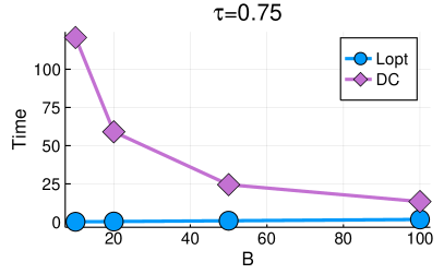
Figure S.6: CPU time (seconds) vs $B$ with $n=1000$. Here ${X}\sim t_{2}$ and the distribution of $Y$ is exponential.

Figure S.7: Empirical MSE vs CPU time (seconds) with $n=1000$ and different values of $B$. Here ${X}\sim t_{2}$ and the distribution of $Y$ is exponential.

References

- Ai et al. (2019) Ai, M., Yu, J., Zhang, H., and Wang, H. (2019). Optimal subsampling algorithms for big data generalized linear models. Statistica Sinica, doi:10.5705/ss.202018.0439.
- Atkinson et al. (2007) Atkinson, A., Donev, A., and Tobias, R. (2007). Optimum Experimental Designs, with SAS. Oxford University Press.
- Battey et al. (2018) Battey, H., Fan, J., Liu, H., Lu, J., and Zhu, Z. (2018). Distributed testing and estimation under sparse high dimensional models. Ann. Statist. 46, 3, 1352–1382.
- Chen and Wei (2005) Chen, C. and Wei, Y. (2005). Computational issues for quantile regression. Sankhyā: The Indian Journal of Statistics 399–417.
- Dhillon et al. (2013) Dhillon, P., Lu, Y., Foster, D. P., and Ungar, L. (2013). New subsampling algorithms for fast least squares regression. In Advances in Neural Information Processing Systems, 360–368.
- Drineas et al. (2012) Drineas, P., Magdon-Ismail, M., Mahoney, M., and Woodruff, D. (2012). Faster approximation of matrix coherence and statistical leverage. Journal of Machine Learning Research 13, 3475–3506.
- Fan et al. (2014) Fan, J., Han, F., and Liu, H. (2014). Challenges of big data analysis. National science review 1, 2, 293–314.
- Fonollosa et al. (2015) Fonollosa, J., Sheik, S., Huerta, R., and Marco, S. (2015). Reservoir computing compensates slow response of chemosensor arrays exposed to fast varying gas concentrations in continuous monitoring. Sensors and Actuators B: Chemical 215, 618–629.
- Goodson (2011) Goodson, D. Z. (2011). Mathematical methods for physical and analytical chemistry. John Wiley & Sons.
- Hjort and Pollard (2011) Hjort, N. L. and Pollard, D. (2011). Asymptotics for minimisers of convex processes. arXiv preprint arXiv:1107.3806 .
- Koenker (2005) Koenker, R. (2005). Quantile regression, vol. 38. Cambridge university press.
- Lin and Xie (2011) Lin, N. and Xie, R. (2011). Aggregated estimating equation estimation. Statistics and Its Interface 4, 73–83.
- Ma et al. (2015) Ma, P., Mahoney, M., and Yu, B. (2015). A statistical perspective on algorithmic leveraging. Journal of Machine Learning Research 16, 861–911.
- Portnoy and Koenker (1997) Portnoy, S. and Koenker, R. (1997). The gaussian hare and the laplacian tortoise: Computation of squared-errors vs. absolute-errors estimators. Statistical Science 1, 279–300.
- Raskutti and Mahoney (2016) Raskutti, G. and Mahoney, M. (2016). A statistical perspective on randomized sketching for ordinary least-squares. Journal of Machine Learning Research 17, 1–31.
- Schifano et al. (2016) Schifano, E. D., Wu, J., Wang, C., Yan, J., and Chen, M.-H. (2016). Online updating of statistical inference in the big data setting. Technometrics 58, 3, 393–403.
- Shang and Cheng (2017) Shang, Z. and Cheng, G. (2017). Computational limits of a distributed algorithm for smoothing spline. The Journal of Machine Learning Research 18, 1, 3809–3845.
- van der Vaart (1998) van der Vaart, A. (1998). Asymptotic Statistics. Cambridge University Press, London.
- Volgushev et al. (2019) Volgushev, S., Chao, S.-K., and Cheng, G. (2019). Distributed inference for quantile regression processes. Ann. Statist. 47, 3, 1634–1662.
- Wang (2019) Wang, H. (2019). More efficient estimation for logistic regression with optimal subsamples. Journal of Machine Learning Research 20, 132, 1–59.
- Wang et al. (2019) Wang, H., Yang, M., and Stufken, J. (2019). Information-based optimal subdata selection for big data linear regression. Journal of the American Statistical Association 114, 525, 393–405.
- Wang et al. (2018) Wang, H., Zhu, R., and Ma, P. (2018). Optimal subsampling for large sample logistic regression. Journal of the American Statistical Association 113, 522, 829–844.
- Yang et al. (2013) Yang, J., Meng, X., and Mahoney, M. (2013). Quantile regression for large-scale applications. In International Conference on Machine Learning, 881–887.
- Yang (2010) Yang, M. (2010). On the de la Garza phenomenon. The Annals of Statistics 38, 2499–2524.