Validation and improvement of the ZPC parton cascade inside a box

Abstract

Cascade solutions of the Boltzmann equation suffer from causality violation at large densities and/or scattering cross sections. Although the particle subdivision technique can reduce the causality violation, it alters event-by-event correlations and fluctuations and is also computationally expensive. Here we evaluate and then improve the accuracy of the ZPC parton cascade for elastic scatterings inside a box without using parton subdivision. We first test different collision schemes for the collision times and ordering time and find that the default collision scheme does not accurately describe the equilibrium momentum distribution at large opacities. We then find a specific collision scheme that can describe very accurately the equilibrium momentum distribution as well as the time evolution towards equilibrium, even at large opacities. We also calculate the shear viscosity and the $\eta/s$ ratio of the parton systems and confirm that the new collision scheme is more accurate. In addition, we use a novel parton subdivision method to obtain the “exact” evolution of the system. This subdivision method is valid for such box calculations and is so much more efficient than the standard subdivision method that we use a subdivision factor of $10^{6}$ in this study.

I Introduction

In high energy heavy ion collisions such as those at the Relativistic Heavy Ion Collider (RHIC) and the Large Hadron Collider (LHC), the quark-gluon plasma (QGP) with deconfined parton degrees of freedom is formed Adams:2005dq ; Adcox:2004mh . Interactions among the partons, which reflect the properties of the QGP, could significantly affect many final state observables such as the hadron spectra, collective flows, and fluctuations He:2015hfa ; Lin:2015ucn ; Ko:2016ioz ; Jin:2018lbk ; Wang:2019vhg . A parton cascade model provides a microscopic description of the space-time evolution of the partonic phase of relativistic heavy ion collisions. Both elastic and inelastic parton cascade models, such as VNI Geiger:1997pf , ZPC Gyulassy:1997zn ; Zhang:1997ej , MPC Molnar:2000jh , and BAMPS Xu:2004mz ; Xu:2007aa , have been constructed to model parton interactions. For example, recent studies from a multi-phase transport (AMPT) model He:2015hfa ; Lin:2015ucn , which includes the ZPC elastic parton cascade Lin:2004en , have shown that even a few parton scatterings in a small system is enough to generate significant momentum anisotropies Bzdak:2014dia ; Li:2016ubw . This concerns the origin of collectivity and the difference between kinetic theory and hydrodynamics in heavy ion collisions, particularly in small systems Nagle:2017sjv ; Kurkela3 . It is therefore important to ensure that the parton cascade solution is accurate in solving the corresponding Boltzmann equation.

The ZPC elastic parton cascade Zhang:1997ej ; Gyulassy:1997zn solves the Boltzmann equation by the cascade method. A scattering happens when the closest distance between two partons is less than the range of interaction $\sqrt{\sigma/\pi}$, where $\sigma$ is the parton scattering cross section. It is well known that causality violation Kodama:1983yk ; Kortemeyer:1995di is inherent in cascade simulations due to the geometrical interpretation of cross section. This leads to inaccurate numerical results at large opacities, i.e., at high densities and/or large scattering cross sections. For example, a recent study Molnar:2019yam has shown that the effect of causality violation on the elliptic flow from the string melting version of the AMPT model Lin:2004en is small but non-zero. This is mainly because the parton density is very high Lin:2014tya even though the cross section is small ($\sim 3$ mb). Causality violation also leads to the fact that different choices of doing collisions and/or the reference frame can lead to different numerical results Zhang:1996gb ; Zhang:1998tj ; Cheng:2001dz . These numerical artifacts due to the causality violation can be reduced or removed by the parton subdivision technique (i.e., the test particle multiplication method) Wong:1982zzb ; Welke:1989dr ; Kortemeyer:1995di ; Pang:1997 ; Zhang:1998tj ; Molnar:2000jh ; Molnar:2001ux ; Molnar:2004yh ; Xu:2004mz . However, parton subdivision alters the event-by-event correlations and fluctuations, the importance of which has been more appreciated in recent years Alver:2010gr ; parton subdivision is also much more computationally expensive.

Therefore the goal of this work is to find a parton cascade algorithm that is accurate enough without using parton subdivision. We investigate different collision schemes for the ZPC parton cascade for elastic scatterings in a box with periodic boundaries and then compare the results with either the theoretical expectation or the “exact” results from ZPC with parton subdivision. The paper is organized as follows. In Sec. II we give a brief introduction to the ZPC parton cascade. We then discuss the parton subdivision technique in Sec. III. Numerical results of the $p_{\rm T}$ distribution and the shear viscosity including the $\eta/s$ ratio for several cases are presented and discussed in Sec. IV. Finally we conclude in Sec. V.

II The ZPC parton cascade

The ZPC parton cascade Zhang:1997ej ; Gyulassy:1997zn includes two-body elastic parton scatterings such as $gg\rightarrow gg$ by solving the Boltzmann equation, where the on-shell phase space density $f(\bm{r},\bm{p},t)$ evolves as

$$p^{\mu}\partial_{\mu}f(\bm{r},\bm{p},t)=\mathcal{C}\left[|\mathcal{M}|^{2}f_{1}(\bm{r}_{1},\bm{p}_{1},t)f_{2}(\bm{r}_{2},\bm{p}_{2},t)\right].$$ (1)

In the above, the collision term $\mathcal{C}[~{}]$ includes the integral over the momenta of the other three partons with an integrand containing factors such as a $\delta$-function for the energy-momentum conservation. The differential cross section of parton scatterings is given by the matrix element as $d\sigma/d\hat{t}\propto|\mathcal{M}|^{2}$.

The default differential cross section in ZPC for two-parton scatterings, based on the gluon elastic scattering cross section as calculated by leading-order QCD, is given by Zhang:1997ej ; Lin:2004en

$$\frac{d\sigma}{d\hat{t}}=\frac{9\pi\alpha_{s}^{2}}{2}\left(1+\frac{\mu^{2}}{\hat{s}}\right)\frac{1}{(\hat{t}-\mu^{2})^{2}},$$ (2)

where $\alpha_{s}$ is the strong coupling constant, $\hat{s}$ and $\hat{t}$ are the standard Mandelstam variables, and $\mu$ is a screening mass to regular the total cross section. This way the total cross section has no explicit dependence on $\hat{s}$ as

$$\sigma=\frac{9\pi\alpha_{s}^{2}}{2\mu^{2}}.$$ (3)

The above Eq.(2) represents forward-angle scatterings. We also test isotropic scatterings in this study, where $d\sigma/d\hat{t}$ is independent of the scattering angle. For this study we take $\alpha_{s}=\sqrt{2/9}$ Zhang:1997ej unless specified otherwise.

In ZPC one can take different choices or collision schemes to implement the cascade method Zhang:1997ej , and ZPC already provides several different choices. With the closest approach criterion for parton scatterings, the closest approach distance may be calculated either in the two-parton center of mass frame or in the global frame of the whole parton system of each event. Two partons may collide when their closest approach distance is smaller than $\sqrt{\sigma/\pi}$, and at a given global time all such possible collisions in the future are ordered in a collision list with the ordering time of each collision, so that they can be carried out sequentially. The collision list is updated continuously after each collision, and for expansion cases the parton system dynamically freezes out when the collision list is empty. For box cases in this work, we terminate the parton cascade at a global time that is large enough so that the parton momentum distribution changes little afterwards. When the closest approach distance is calculated in the two-parton center of mass frame, the collision time of a scattering in that frame is a well-defined single value. However, because of the finite $\sigma$ the two partons have different spatial coordinates in general, therefore this collision time in the two-parton center of mass frame becomes two different colliding times in the global frame (named here as $ct_{1}$ and $ct_{2}$ respectively for the two colliding partons) after the Lorentz transformation. Note that each of the two partons involved in a scattering changes its momentum at its collision time at the corresponding position in the global frame.

We show in Table 1 a dozen different collision schemes for the case of calculating the closest approach distance in the two-parton center of mass frame, where a collision scheme refers to a given choice of the collision time(s) and the ordering time. These schemes include the ones that choose the collision time(s) in the global frame as separate values (i.e., as $ct_{1}$ and $ct_{2}$), the earlier time $min(ct_{1},ct_{2})$, the average time $(ct_{1}+ct_{2})/2$, or the later time $max(ct_{1},ct_{2})$, in combination with choosing the collision ordering time in the global frame as either the earlier time, the average time, or the later time. On the other hand, for the case of calculating the closest approach distance in the global frame, it is natural to choose the single collision time as the collision ordering time (both in the global frame); this is called collision scheme M here.

Table 1: Different collision schemes for ZPC when the closest approach distance is calculated in the two-parton center of mass frame. $ct_{1}$ and $ct_{2}$ represent the collision times of the two scattered partons after the transformation back to the global frame.

	$ct_{1}$ & $ct_{2}$	$min(ct_{1},ct_{2})$	$(ct_{1}+ct_{2})/2$	$max(ct_{1},ct_{2})$
$min(ct_{1},ct_{2})$	A	B (new scheme)	C	D
$(ct_{1}+ct_{2})/2$	E	F	G (default ZPC scheme)	H
$max(ct_{1},ct_{2})$	I	J	K	L

We first test these different collision schemes for the case of 4,000 massless gluons in a box with a cross section of $\sigma=2.6$ mb for forward-angle scatterings. The box size is chosen such that the gluon density $n$ is the same as that for a thermalized gluon system at the temperature $T=0.5$ GeV, i.e., $n=d_{g}T^{3}/\pi^{2}$ with the gluon degeneracy factor $d_{g}=16$. Since we do not include quantum statistics in the collision kernel of Eq.(1), the final state momentum distribution of the gluon system should be given by the Maxwell$\textendash$Boltzmann distribution at this temperature.

We use an off-equilibrium initial condition that is uniform in the coordinate space, which is obtained by first generating the Maxwell$\textendash$Boltzmann momentum distribution and then decreasing each parton’s initial $p_{z}$ by a factor of two while keeping its initial 3-momentum the same. Such off-equilibrium initial momentum distribution is used for all the calculations of the $p_{\rm T}$ spectra in Sec. IV.1, while the equilibrium initial momentum distribution is used for calculations of shear viscosity in Sec. IV.2. Also note that the ZPC results in this study are obtained without using parton subdivision unless specified otherwise, and typically a few thousand events is used for each case while each event simulates the scatterings of at least 4,000 massless gluons. The number of gluons for each case is chosen so that the cell size in ZPC is no smaller than the interaction length to ensure the numerical accuracy.

Figure 1 shows the final $p_{\rm T}$ distributions from different collision schemes for the above case in comparison with the initial distribution (thin solid curve) and the expected final state distribution (thick solid curve). Note that each final distribution in Fig. 1 is obtained by running the ZPC parton cascade for a global time of 6.1 fm$/c$, when the $p_{\rm T}$ distribution has become very stable (as can be seen from Fig.5). We see that the numerical solution of ZPC depends significantly on the collision scheme in this case. In addition, the distributions from collision schemes with the same ordering time (i.e., schemes A to D, or schemes E to H, or schemes I to L) are relative close to each other. Collision scheme G, which uses $(ct_{1}+ct_{2})/2$ as both the collision time and ordering time, is the default collision scheme of ZPC Zhang:1997ej and also used in the AMPT model  Lin:2004en , so we label it as default ZPC in this study. We see that the final $p_{\rm T}$ distribution from the default ZPC scheme in Fig. 1 deviates considerably from the expected thermal distribution, and so do the results from most collision schemes. However, the final $p_{\rm T}$ distribution from collision scheme B, which uses $min(ct_{1},ct_{2})$ as both the collision time and ordering time, is the closest to the expected thermal distribution. Therefore we focus on collision scheme B and call it the new scheme.

Currently our finding that the collision scheme using time $min(ct_{1},ct_{2})$ best preserves the equilibrium momentum distribution is a numerical observation. More generally the ordering time or the collision time in the global frame can be chosen as a function of $ct_{1}$ and $ct_{2}$. Indeed we could fine-tune the new collision scheme by choosing a point (near $min(ct_{1},ct_{2})$) on the linear interpolation line between $ct_{1}$ and $ct_{2}$ to preserve the equilibrium momentum distribution even better. Causality violation usually suppresses the collision rates, which is the case for the default ZPC scheme as shall be shown in Fig. 3. Therefore we can expect that choosing time $min(ct_{1},ct_{2})$ instead of $(ct_{1}+ct_{2})/2$ enhances the collision rates and alleviates the effect of causality violation. Other than this, we find no clear theoretical arguments on why the new scheme works better to suppress the causality violation. It may be related to correlated functions in theories such as the Kadanoff-Baym equations Lipavsky:1986zz ; Semkat . However, the various collision schemes in Table 1 are only different at finite opacities, where causality violation complicates the theoretical analysis of different schemes.

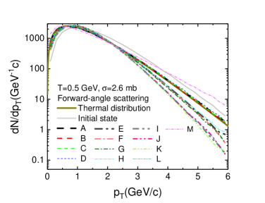
Figure 1: The final $p_{\rm T}$ distributions from different collision schemes for elastic gluon scatterings in a box with $T=0.5$ GeV and forward-angle scatterings at $\sigma=2.6$ mb.

III Parton subdivision

Naively a parton cascade is only correct in the dilute limit to preserve causality and Lorentz covariance  Zhang:1998tj ; Molnar:2000jh ; Molnar:2001ux ; Cheng:2001dz , where the particle range of interaction is much smaller than the mean free path. Their ratio can be written as Zhang:1998tj

$$\chi=\sqrt{\frac{\sigma}{\pi}}/\lambda=n\sqrt{\frac{\sigma^{3}}{\pi}},$$ (4)

where $n$ is the parton density and $\lambda$ is the mean free path. We can use $\chi$ to represent the opacity of the parton system, and the dilute limit means $\chi\ll 1$. Above the dilute limit, a parton cascade may suffer from the causality violation Kodama:1983yk ; Kortemeyer:1995di ; Zhang:1996gb ; Zhang:1998tj ; Cheng:2001dz , which is an artifact of the geometrical interpretation of cross section in the cascade method. This is why we see the differences in the numerical solutions from difference collision schemes in Fig. 1, which case corresponds to $\chi=2.0$.

The parton subdivision technique Pang:1997 ; Zhang:1998tj can be used to reduce the numerical artifact from the causality violation, and the numerical solution of a parton cascade will be correct in the limit of large parton subdivision factor. This is because the Boltzmann equation in Eq.(1) may be expressed as

$$p^{\mu}\partial_{\mu}f(\bm{r},\bm{p},t)\propto\sigma f_{1}(\bm{r}_{1},\bm{p}_{1},t)f_{2}(\bm{r}_{2},\bm{p}_{2},t).$$ (5)

Therefore the following transformation keeps the above equation invariant:

$$f(\bm{r},\bm{p},t)\rightarrow l\times f(\bm{r},\bm{p},t),~{}~{}~{}\sigma\rightarrow\sigma/l;$$ (6)

but it reduces the opacity as

$$\chi\rightarrow\chi/\sqrt{l}.$$ (7)

In the above, $l$ is the subdivision factor, typically an integer much greater than one. Therefore at large enough $l$ the transformed parton system will reach the dilute limit and thus the cascade solution for its evolution will be accurate.

We emphasize that the angular distribution of the cross section must not be changed when performing the above subdivision transformation Eq. (6) to ensure the invariance of the Boltzmann equation; this can be clearly seen from the term $|\mathcal{M}|^{2}$ in Eq.(1). Therefore the exact transformation for parton subdivision is the following:

$$f(\bm{r},\bm{p},t)\rightarrow l\times f(\bm{r},\bm{p},t),~{}~{}~{}\frac{d\sigma}{d\hat{t}}\rightarrow\frac{d\sigma}{d\hat{t}}/l.$$ (8)

This is especially relevant for forward-angle scatterings, because there the total cross section as well as the angular distribution are determined by the screening mass $\mu$ as shown in Eqs.(2-3). When parton subdivision requires the decrease of the forward-angle cross section of Eq.(3), one should not do that by increasing $\mu$ by a factor of $\sqrt{l}$ because that would change the angular distribution of the scatterings. Instead one can decrease the $\alpha_{s}$ parameter by a factor of $\sqrt{l}$ in Eqs.(2-3), which decreases the total scattering cross section while keeping its angular distribution.

In the standard subdivision method one increases the initial parton number per event by factor $l$ while decreasing the cross section by the same factor. This method can be schematically represented by the following transformation:

$$N\rightarrow l\times N,V{~{}\rm unchanged},$$ (9)

where $N$ is the initial parton number in an event and $V$ is the initial volume of the parton system. For box calculations of elastic scatterings in this study, of course the parton number in an event and the volume do not change with time. Since the number of possible collisions scales with $l^{2}$, the subdivision method is very expensive in terms of the computation time, which roughly scales with $l^{2}$ per subdivision event or with $l$ per simulated parton. However, for box calculations where the density function $f(\bm{r},\bm{p},t)$ is spatially homogeneous, we can realize parton subdivision with a different method. This new subdivision method can be schematically represented by

$$N{~{}\rm unchanged},V\rightarrow V/l,$$ (10)

where we decrease the volume of the box by factor $l$ while keeping the same parton number and momentum distribution in each event. Because the parton number per event does not change, this subdivision method is much more efficient than the standard subdivision method, therefore we can afford a huge subdivision factor such as $10^{6}$ (instead of the usual value of up to a few hundreds). For all parton subdivision calculations in this study, we shall use this new subdivision method with $l=10^{6}$ under the default ZPC scheme (unless specified otherwise).

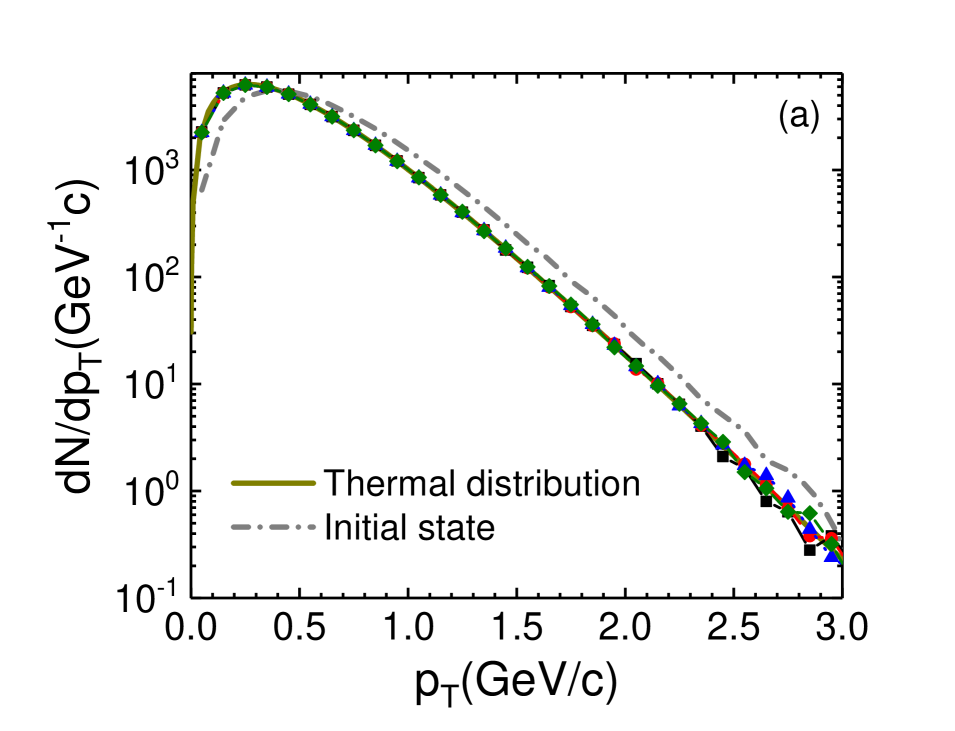
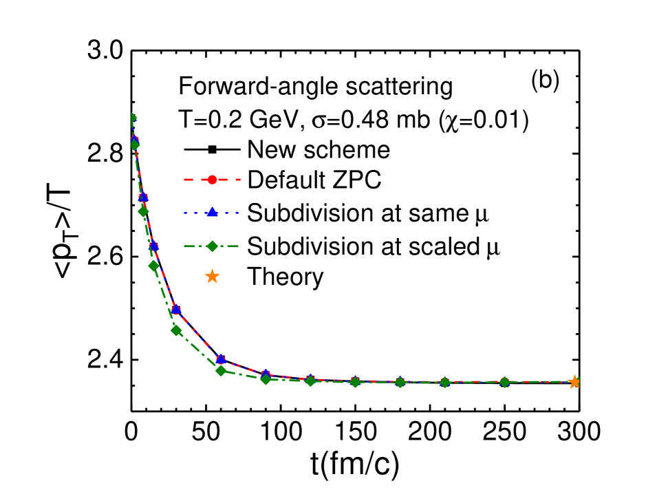
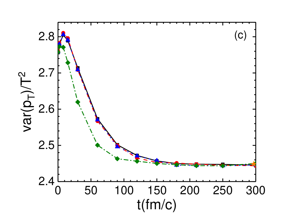
Figure 2: (a) The final $p_{\rm T}$ distribution, (b) time evolution of $\langle p_{\rm T}\rangle/T$, and (c) time evolution of var($p_{\rm T}$)$/T^{2}$ from the new scheme, the default ZPC scheme, and two parton subdivision methods in a low-opacity test at $\alpha_{s}=0.20$, $T=0.2$ GeV for forward-angle scatterings at $\sigma=0.48$ mb. The star symbols represent the theoretical values at late times.

To explicitly show the importance of keeping the same scattering angular distribution when implementing the parton subdivision method, as shown by Eq.(8), we apply the ZPC parton cascade to a dilute limit. For this case we simulate for each event 4,000 gluons at $T=0.2$ GeV with an off-equilibrium momentum distribution. We set $\mu=3.47$ fm^-1 and $\alpha_{s}=0.201$, which then gives a forward-angle scattering cross section $\sigma=0.48$ mb and $\chi=0.01$ (a dilute system). Figure 2 shows the results of the final $p_{\rm T}$ distribution, time evolution of $\langle p_{\rm T}\rangle/T$, and time evolution of var($p_{\rm T}$)$/T^{2}$ from different cascade methods, where $\langle p_{\rm T}\rangle$ is the mean transverse momentum of each parton and

$${\rm var}(p_{\rm T})=\langle{p_{\rm T}^{2}}\rangle-\langle p_{\rm T}\rangle^{2}$$ (11)

is the variance of the final $p_{\rm T}$ distribution. The results include those from the new scheme, the default ZPC scheme, the parton subdivision method at $l=10^{6}$ with an unchanged scattering angular distribution (i.e., by decreasing $\alpha_{s}$ while keeping $\mu$ the same), and the parton subdivision method at $l=10^{6}$ with a changed scattering angular distribution (i.e., by increasing $\mu$). Note that these two parton subdivision calculations are performed with the default ZPC scheme; however, the choice of schemes no longer affects the numerical results here because the large $l$ value for the parton subdivision has essentially eliminated the causality violation.

We first see in Fig. 2 that the results from the new scheme (solid curves) and the default ZPC scheme (dashed curves) agree with each other very well; this is because the effect of causality violation and thus the dependence on the collision scheme is very small in this dilute limit. We also see that they agree with the parton subdivision method that keeps the same scattering angular distribution (dotted curves) but their time evolutions disagree with the parton subdivision method that changes the scattering angular distribution (dot-dashed curves), thus verifying the parton subdivision method of Eq.(8). From now on we shall use this method for parton subdivision for all the remaining calculations. In addition, the time evolutions of $\langle p_{\rm T}\rangle$ and ${\rm var}(p_{\rm T})$ are both faster for the parton subdivision method that changes the scattering angular distribution; this is because the subdivision scaling $\mu\rightarrow\sqrt{l}~{}\mu$ used in this “wrong” subdivision method makes the angular distribution more isotropic and thus leads to a higher transport cross section Molnar:2001ux than the “correct” subdivision method (dotted curves). The star symbols in Figs. 2(b) and 2(c) represent the theoretical values at late times (or in equilibrium) for the mean value (scaled by $1/T$) and the variance (scaled by $1/T^{2}$) of the $p_{\rm T}$ distributions, respectively, where

$$\langle p_{\rm T}\rangle=\frac{3\pi T}{4},~{}~{}{\rm var}(p_{\rm T})=\left(8-\frac{9\pi^{2}}{16}\right)T^{2}.$$ (12)

At late times all four ZPC calculations in Fig. 2 reach the correct equilibrium values for this dilute case.

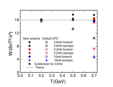
Figure 3: Scaled collision rates per unit volume $W$ as functions of temperature $T$ for forward-angle scatterings and isotropic scatterings at different cross sections. Results from the new scheme and the default ZPC scheme are compared with the parton subdivision results and the theoretical value.

We also check the collision rates per volume Zhang:1998tj in Fig. 3, which shows the results for cases with different cross sections and temperatures for both forward-angle and isotropic scatterings. The horizontal line represents the (scaled) expected rate per volume for a massless gluon system in equilibrium, which is given by Zhang:1998tj

$$W=\frac{8\sigma T^{6}}{\pi^{4}}F\left(\frac{2m}{T}\right)\textrm{~{}~{}~{}with~{}~{}~{}}F(x)=\int_{x}^{\infty}dyy^{2}(y^{2}-x^{2})K_{1}(y),$$ (13)

In the above, $K_{1}(y)$ is the modified Bessel function, and $F(0)=16$ for massless gluons that we consider in this study. We see that as expected the small-opacity results (symbols at $T=0.2$ GeV) from the new scheme and the default ZPC scheme for both forward-angle and isotropic scatterings are almost the same. For large opacities, however, the results (symbols at $T=0.5$ GeV and $0.7$ GeV) depend significantly on the collision scheme; they also depend on the scattering angular distribution in some cases. In particular, the collision rate per volume from the default ZPC scheme gets much lower than the theoretical expectation for large cross sections or parton densities (which scales as $T^{3}$). On the other hand, the collision rates per volume from the new scheme are much closer to the theoretical value, even at large opacities. Also, it is no surprise that the parton subdivision results agree with the theoretical expectation. Note that the collision rates per unit volume are essentially the same when we use the equilibrium initial condition instead of the off-equilibrium initial condition.

IV Main results and discussions

IV.1 The $p_{\rm T}$ distribution and its time evolution

We now use different cases to test the new collision scheme in comparison with the default ZPC scheme and exact results on the momentum distribution. As noted before, the initial momentum distribution in each of these calculations is off-equilibrium so that we can better observe the time evolution and equilibration of the momentum distribution.

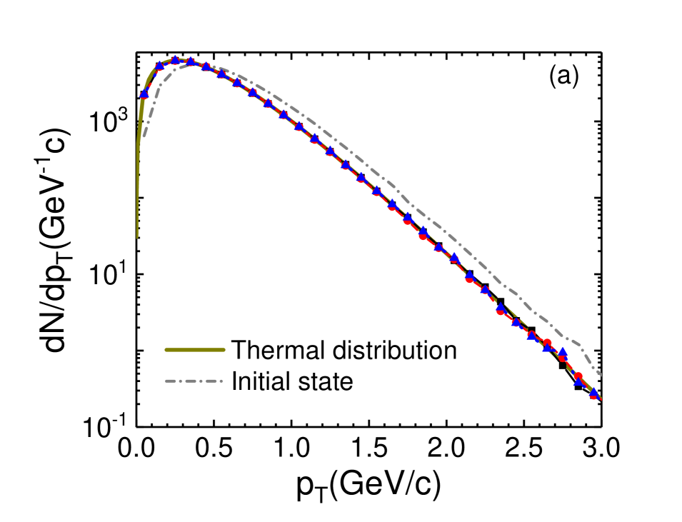
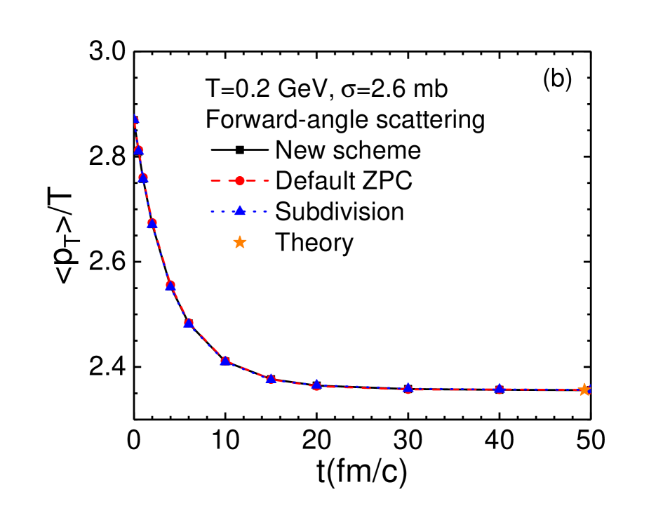
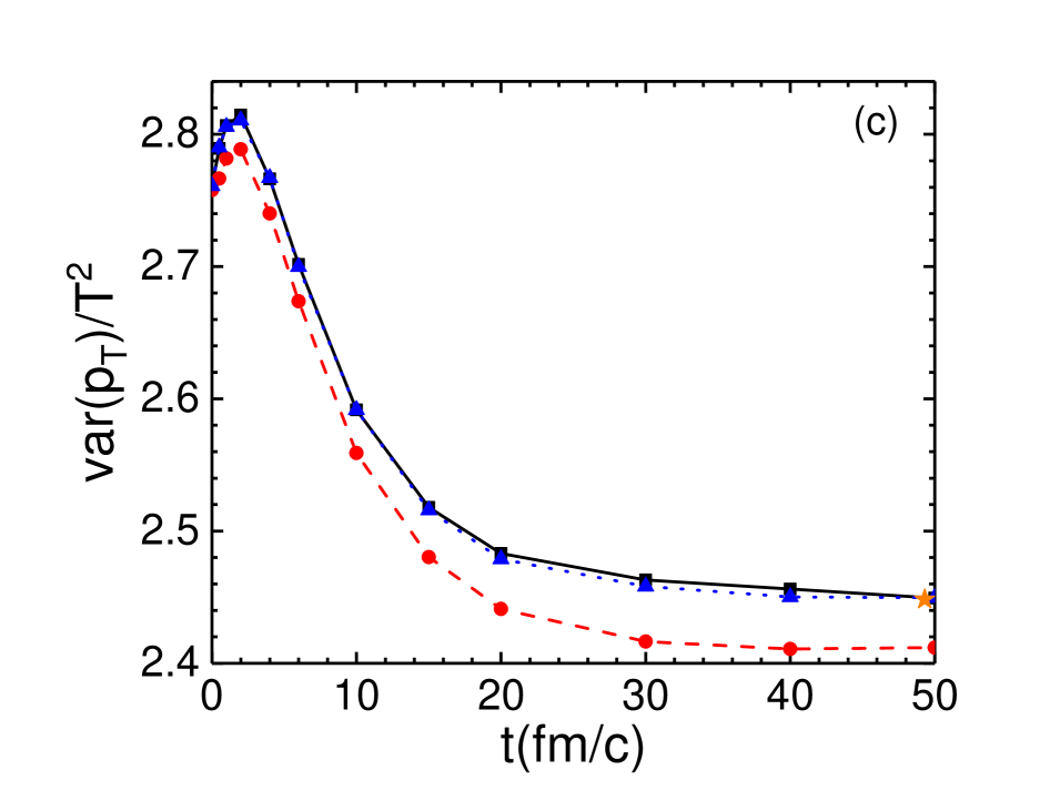
Figure 4: (a) The final $p_{\rm T}$ distributions, (b) time evolutions of $\langle p_{\rm T}\rangle/T$, and (c) time evolutions of var($p_{\rm T}$)$/T^{2}$ from the new scheme and the default ZPC scheme in comparison with the parton subdivision results in a box at $T=0.2$ GeV for forward-angle scatterings at $\sigma=2.6$ mb ($\chi=0.13$).

We start with a test of forward-angle scatterings at low opacity, where $\sigma=2.6$ mb and $T=0.2$ GeV that correspond to $\chi=0.13$. Figure 4 shows the final $p_{\rm T}$ distributions, the time evolutions of $\langle p_{\rm T}\rangle/T$, and the time evolutions of var($p_{\rm T}$)$/T^{2}$. In Fig. 4(a) we see no obvious difference between the final $p_{\rm T}$ distributions of the three methods of doing the parton cascade, i.e., the new scheme, the default ZPC scheme, and the parton subdivision method at $l=10^{6}$. They are also consistent with the thermal distribution, which is expected because the small $\chi$ value here means that the effect from causality violation should be quite small. Furthermore, the time evolutions of the mean transverse momentum in Fig. 4(b) also show little difference among the three methods. However, we observe some difference in the time evolutions of the variance of the $p_{\rm T}$ distributions in Fig. 4(c); in particular, the variance from the default ZPC scheme is obviously smaller than the other two results soon after the start of parton cascade, meaning that the $p_{\rm T}$ distribution from the default ZPC scheme is somewhat narrower in width, even at late times. In addition, Figs. 4(b) and 4(c) indicate that the $p_{\rm T}$ distributions from the new scheme and from the parton subdivision method follow a similar time evolution and at late times they agree with the theoretical expectations (star symbols).

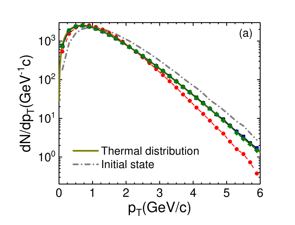
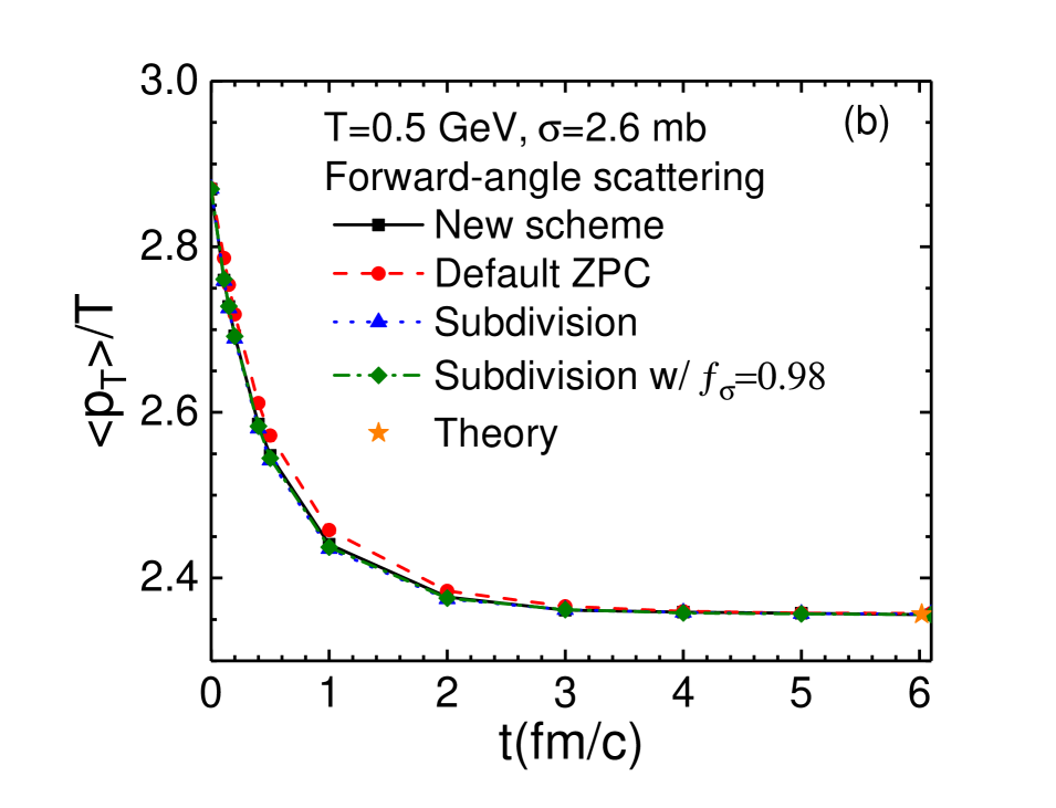
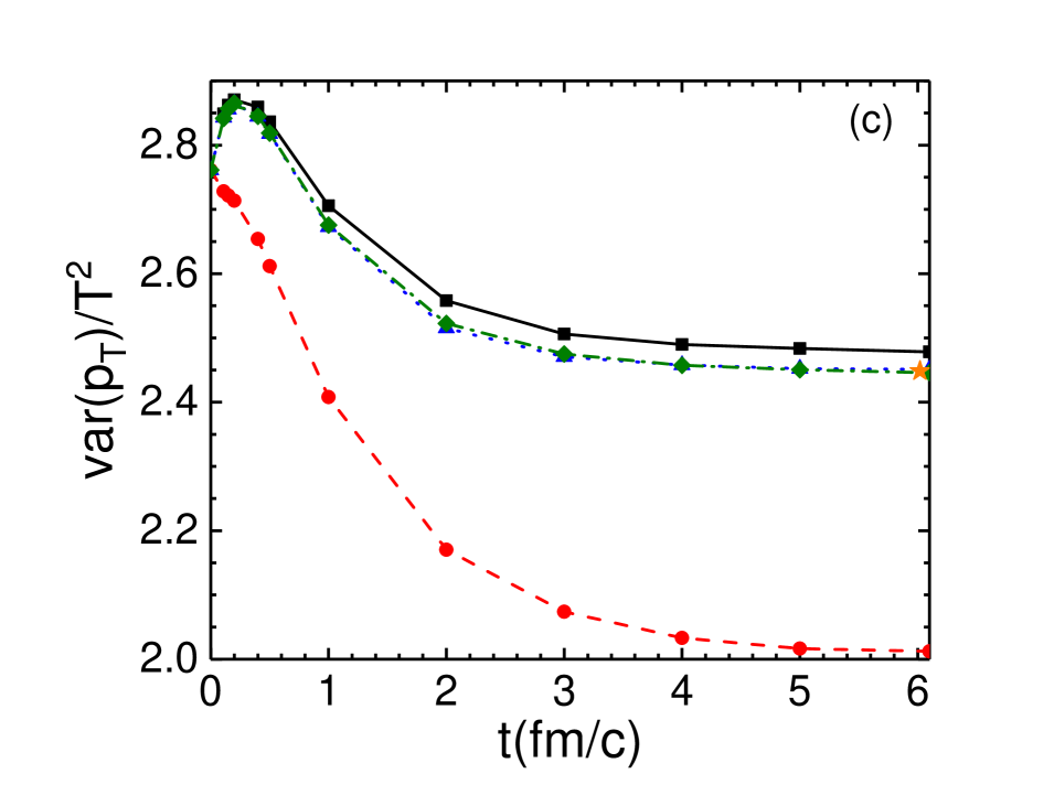
Figure 5: Same as Fig. 4 but at $T=0.5$ GeV for forward-angle scatterings at $\sigma=2.6$ mb ($\chi=2.0$).

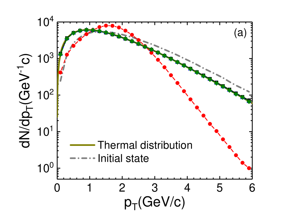
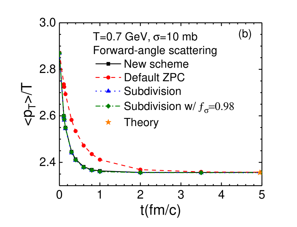
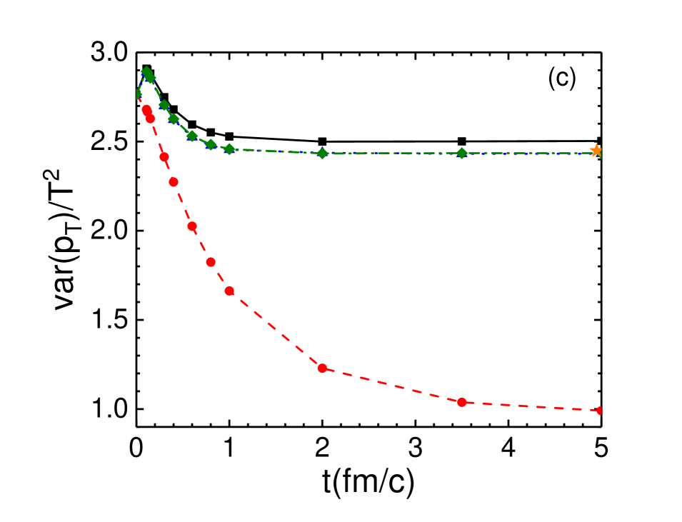
Figure 6: Same as Fig. 4 but at $T=0.7$ GeV for forward-angle scatterings at $\sigma=10$ mb ($\chi=41$).

The results of two cases of higher opacities, one at $T=0.5$ GeV and $\sigma=2.6$ mb, another at $T=0.7$ GeV and $\sigma=10$ mb, for forward-angle scatterings are shown in Fig. 5 and Fig. 6, respectively. The first case as shown in Fig. 5 corresponds to $\chi=2.0$; we see that the $p_{\rm T}$ distribution and its variance from the default ZPC scheme both deviate significantly from the “exact” parton subdivision results, although the time evolutions of $\langle p_{\rm T}\rangle$ are close to each other. On the other hand, results from the new scheme are very close to the parton subdivision results, which agree with theoretical expectations at late times. The second case as shown in Fig. 6 corresponds to $\chi=41$, which serves as an example of extreme opacity. We see qualitatively the same features as seen in Fig. 5, but the results from the default ZPC scheme are now much further away from the parton subdivision results, including its time evolution of $\langle p_{\rm T}\rangle$. Again, results from the new scheme are quite close to the subdivision results or the theoretical expectations even at this extreme opacity.

We have also tested isotropic scatterings and reached similar conclusions. As an example, Fig. 7 shows the results for isotropic scatterings for the case of $T=0.5$ GeV and $\sigma=2.6$ mb (i.e., $\chi=2.0$). We see the same features as those shown in Fig. 5 for forward-angle scatterings, e.g., the results of the new scheme are close to the subdivision results while the default ZPC scheme gives very different results that are far from the theoretical expectations at late times. Therefore we conclude that for box calculations the new collision scheme (i.e., scheme B in Table 1) is very accurate over a large range of opacities and much better than the default ZPC collision scheme.

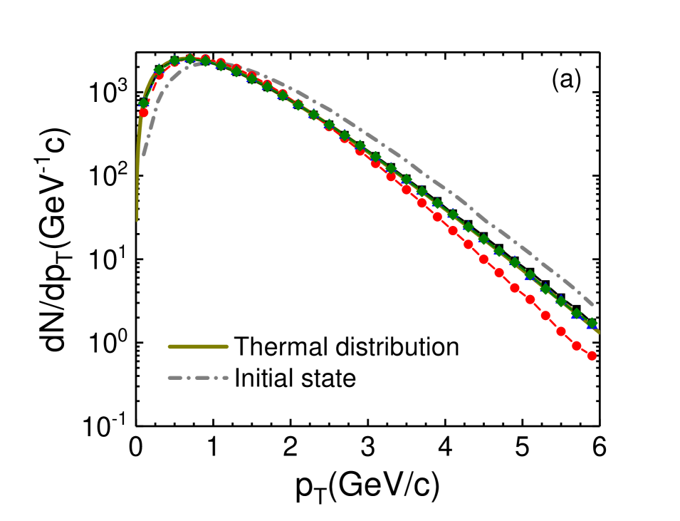
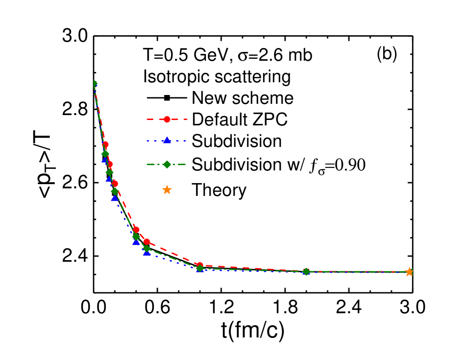
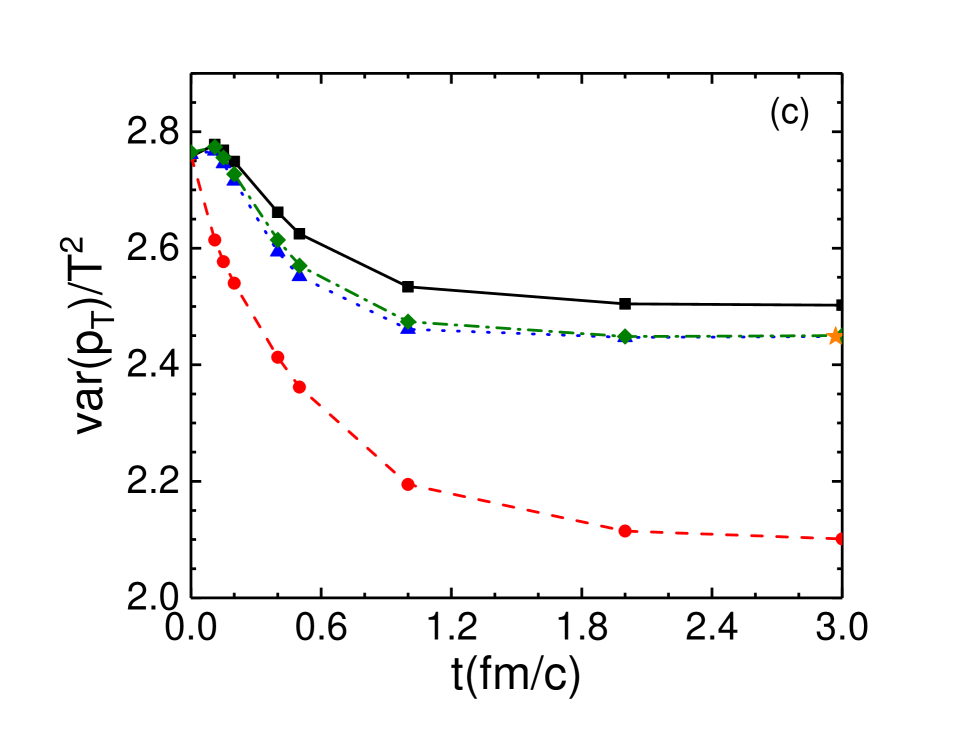
Figure 7: Same as Fig. 5 but for isotropic scatterings.

To characterize the accuracy of the final $p_{\rm T}$ distribution from the new collision scheme, we may compare the final $\langle p_{\rm T}\rangle/T$ and ${\rm var}(p_{\rm T})/T^{2}$ with the corresponding theoretical values in Eq. (12). However, we can see from the figures that the final $\langle p_{\rm T}\rangle$ value at late times from every box calculation in this study agrees with Eq. (12); this is due to the momentum isotropy in equilibrium and the energy conservation because the average energy per parton ($3T$) does not depend on the collision scheme or method. Therefore we choose to use the ratio between the final ${\rm var}(p_{\rm T})/T^{2}$ value and the theoretical value to represent the accuracy of the new collision scheme. The values of this ratio for different cases are shown in Fig. 8 as functions of the opacity parameter $\chi$. We see that the ratio is essentially unity at low opacities, indicating that there the new scheme is very accurate as expected. At moderate to high opacities, the deviations of the variance of the $p_{\rm T}$ distribution are quite small, up to about 3%. Also, an interesting feature for isotropic scatterings is that the maximum deviation in the variance does not occur at the highest opacity shown but at a moderate opacity.

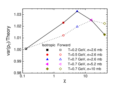
Figure 8: The ratio between the final var($p_{\rm T}$) from the new scheme and the theoretical value versus the opacity parameter $\chi$ for different cases.

We see from Figs. 5-7 that the time evolutions of $\langle p_{\rm T}\rangle$ from the new scheme (dashed curves) are somewhat different from the parton subdivision results, although the $\langle p_{\rm T}\rangle$ values at late times agree well with the theoretical value of Eq. (12). Therefore we may ask the question: at what equivalent cross section will the parton subdivision method give the same time evolution of $\langle p_{\rm T}\rangle$ as the new scheme? For example, Fig. 7(b) shows that the time evolution from the new scheme (solid curve) is slower than the subdivision result at the same cross section of 2.6 mb (dotted curve); thus we expect that the subdivision result at a smaller cross section could better match the time evolution of the new scheme. For this purpose, we can write schematically a new subdivision transformation:

$$f(\bm{r},\bm{p},t)\rightarrow l\times f(\bm{r},\bm{p},t),~{}~{}~{}\frac{d\sigma}{d\hat{t}}\rightarrow f_{\sigma}\times\frac{d\sigma}{d\hat{t}}/l,$$ (14)

where $f_{\sigma}$ is the effectiveness factor of cross section. We then determine the $f_{\sigma}$ factor by minimizing the difference between the time evolution from the new scheme and that from the above parton subdivision method. More specifically, we minimize the average absolute difference between the $\langle p_{\rm T}\rangle$ values at about a dozen selected time points from the new scheme and the corresponding $\langle p_{\rm T}\rangle$ values from the subdivision method of Eq. (14), where the selected time points are usually taken as the positions of the symbols on the curves from the new scheme in Figs. 4-7.

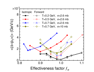
Figure 9: The average absolute difference in $\langle p_{\rm T}\rangle$ versus $f_{\sigma}$, the effectiveness factor of cross section, for different cases.

Figure 9 shows the average absolute difference in $\langle p_{\rm T}\rangle$ versus the $f_{\sigma}$ value for several different cases, where we can find the minimum position for each case. The optimal $f_{\sigma}$ value, i.e., the value that gives the minimum $\langle p_{\rm T}\rangle$ difference, is given for each case in Table 2. We can see that the optimal $f_{\sigma}$ value is 1.00 for the low opacity case (at $T=0.2$ GeV and $\sigma=2.6$ mb), which is expected because of the small causality violation. On the other hand, the biggest deviation of the optimal $f_{\sigma}$ from unity occurs for the case of isotropic scatterings at a moderate opacity (at $T=0.7$ GeV and $\sigma=2.6$ mb). Note that this is also the case with the largest deviation of the final ${\rm var}(p_{\rm T})/T^{2}$ value from the theoretical value, as can be seen in Fig. 8. Also shown in Figs. 5-7 are the results from the subdivision method of Eq. (14) after using the corresponding optimal $f_{\sigma}$ values (dot-dashed curves), which nicely match the time evolutions of $\langle p_{\rm T}\rangle$ from the new scheme. For example, the optimal value $f_{\sigma}=0.93$ in Fig. 6 means that the new collision scheme for forward-angle scatterings at $\sigma=10$ mb (and $T=0.7$ GeV) is effectively equivalent to the “exact” parton subdivision method that uses the cross section $\sigma=9.3$ mb (with the same scattering angular distribution).

Table 2: $f_{\sigma}$, the effectiveness factor of cross section, for different cases.

T & $\sigma$ values	0.2 GeV & 2.6 mb	0.5 GeV & 2.6 mb	0.7 GeV & 2.6 mb	0.7 GeV & 10 mb
	($\chi=0.13$)	($\chi=2.0$)	($\chi=5.5$)	($\chi=41.$)
$f_{\sigma}$ for forward-angle scatterings	1.00	0.98	0.98	0.98
$f_{\sigma}$ for isotropic scatterings	1.00	0.90	0.84	0.98

IV.2 Shear viscosity and the $\eta/s$ ratio

Transport coefficients such as the shear viscosity $\eta$ represent important properties of the created matter Schafer:2009dj . It is thus useful to evaluate the effect of our new collision scheme on the shear viscosity $\eta$ and its ratio over the entropy density $\eta/s$. The Green-Kubo relation Green ; Kubo has been applied Muronga:2003tb ; Demir:2008tr ; Fuini:2010xz ; Wesp:2011yy ; Li:2011xu to calculate the shear viscosity at or near equilibrium. Therefore we start with an equilibrium initial condition for shear viscosity calculations in this section.

We calculate the shear viscosity according to the following form of the Green-Kubo relation Muronga:2003tb :

$$\eta=\frac{V}{T}\int_{0}^{\infty}dt\,\langle\bar{\pi}^{xy}(t+t^{\prime})\,\bar{\pi}^{xy}(t^{\prime})\rangle.$$ (15)

Here $\langle...\rangle$ represents the time ($t^{\prime}$) and ensemble average, and $\bar{\pi}^{xy}(t)$ represents the volume averaged $xy$-component of the energy momentum tensor $\pi^{\mu\nu}$:

$$\pi^{\mu\nu}({\bm{r}},t)=\frac{1}{(2\pi)^{3}}\int d^{3}p\frac{p^{\mu}p^{\nu}}{p^{0}}f(\bm{r},\bm{p},t).$$ (16)

Since we do not consider parton potentials in the ZPC parton cascade here, the volume average of $\pi^{xy}$ at a given time $t$ can be written as

$$\bar{\pi}^{xy}(t)=\frac{1}{V}\sum_{i=1}^{N}\frac{p_{i}^{x}p_{i}^{y}}{p^{0}_{i}},$$ (17)

where the sum is over all partons in the box at time $t$.

It is known that the correlation function in Eq. (15) damps exponentially with time Muronga:2003tb ; Demir:2008tr ; Wesp:2011yy :

$$\langle\bar{\pi}^{xy}(t+t^{\prime})\,\bar{\pi}^{xy}(t^{\prime})\rangle=\langle\bar{\pi}^{xy}(t^{\prime})\,\bar{\pi}^{xy}(t^{\prime})\rangle~{}e^{-t/\tau}$$ (18)

with $\tau$ being the corresponding relaxation time. Also, the average variance of $\bar{\pi}^{xy}$ in equilibrium is given by

$$\langle\bar{\pi}^{xy}(t^{\prime})\,\bar{\pi}^{xy}(t^{\prime})\rangle=\frac{4}{15}\frac{\epsilon\,T}{V},$$ (19)

where $\epsilon=3d_{g}T^{4}/\pi^{2}$ is the energy density of massless gluons in equilibrium. We then have

$$\eta=\frac{4}{15}\,\epsilon\,\tau.$$ (20)

So we extract the relaxation time $\tau$ from the calculation of the correlation function in Eq. (18). Specifically, the time and ensemble average of the correlation function in our numerical calculations is obtained as Muronga:2003tb ; Wesp:2011yy

$$\langle\bar{\pi}^{xy}(t+t^{\prime})\,\bar{\pi}^{xy}(t^{\prime})\rangle=\left\langle\frac{1}{T_{t}}\int_{0}^{T_{t}}\bar{\pi}^{xy}(t+t^{\prime})\,\bar{\pi}^{xy}(t^{\prime})\,dt^{\prime}\right\rangle\simeq\left\langle\frac{1}{N_{t}}\sum_{j=0}^{N_{t}-1}\bar{\pi}^{xy}(i\Delta t+j\Delta t)\,\bar{\pi}^{xy}(j\Delta t)\right\rangle.$$ (21)

In the above, $N_{t}=T_{t}/\Delta t$, $t=i\Delta t$, and each of the last two $\langle...\rangle$ symbols represents the ensemble average. Here we typically choose $T_{t}\sim 30\tau,N_{t}\sim 200$, and extract $\tau$ from a fit to the normalized correlation function over the the range $t\in[0,\sim\!2\tau]$. Note that $\langle\bar{\pi}^{xy}(t+t^{\prime})\,\bar{\pi}^{xy}(t^{\prime})\rangle$ is often abbreviated as $\langle\bar{\pi}^{xy}(t)\,\bar{\pi}^{xy}(0)\rangle$ in studies that use the Green-Kubo relation Muronga:2003tb ; Demir:2008tr ; Fuini:2010xz ; Wesp:2011yy ; Li:2011xu . In addition, for isotropic elastic collisions the shear viscosity and the corresponding relaxation time of a massless Maxwell$\textendash$Boltzmann gas in equilibrium can be calculated in the Navier-Stokes approximation as DeGroot:1980dk ; Huovinen:2008te

$$\eta^{N\!S}\simeq 1.265\,\frac{T}{\sigma},~{}\tau^{N\!S}\simeq\frac{1.582}{n\sigma}.$$ (22)

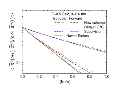
Figure 10: Normalized correlation functions from different collision schemes for isotropic scatterings and forward-angle scatterings at $T=0.5$ GeV and $\sigma=2.6$ mb; the solid line represents the Navier-Stokes expectation for isotropic scatterings.

We show in Fig. 10 the normalized correlation functions for the case of $T=0.5$ GeV and $\sigma=2.6$ mb, which corresponds to opacity $\chi=2.0$. All the numerical results show the expected exponential damping with time. For isotropic scatterings, we see that the result from the subdivision method is almost the same as the Navier-Stokes expectation. On the other hand, the ZPC result without parton subdivision using the new collision scheme or the default collision scheme both damps a bit more slowly, which will lead to a bit larger relaxation time and $\eta$ value than those from the parton subdivision method. For forward-angle scatterings, Fig. 10 also shows that the ZPC results without parton subdivision damp a bit more slowly than the result from parton subdivision. Furthermore, for both isotropic and forward-angle scatterings, the damping rates from the new scheme are closer to the subdivision results than those from the default scheme.

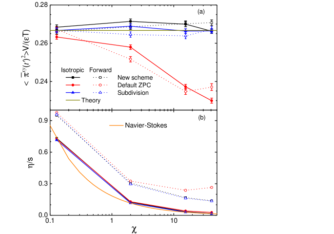
Figure 11: (a) Scaled average variance $\langle\bar{\pi}^{xy}(t^{\prime})\,\bar{\pi}^{xy}(t^{\prime})\rangle$ (with statistical error bars) versus opacity $\chi$ for different cases in comparison with the theoretical value for equilibrium (solid line). (b) The $\eta/s$ ratio for different cases versus opacity; the solid curve represents the Navier-Stokes expectation for isotropic scatterings.

We also check our results of the average variance $\langle\bar{\pi}^{xy}(t^{\prime})\,\bar{\pi}^{xy}(t^{\prime})\rangle$ in Fig. 11(a) from different cases for both isotropic and forward-angle scatterings. The average variance has been multiplied by the factor $V/(\epsilon\,T)$ because then its theoretical value is 4/15 (solid line). The cases included in Fig. 11 are the same as those shown in Fig. 8 except for the omission of the case of $T=0.7$ GeV with $\sigma=2.6$ mb (at $\chi=5.5$). We see that in general the results from the subdivision method agree well with the theoretical expectation from low to very high opacities. The results from the new collision scheme also agree with the theoretical value rather well. On the other hand, the average variance from the default ZPC collision scheme deviates significantly from the theoretical value at finite opacities (up to $\sim 16\%$ at the extreme opacity of $\chi=41$).

Figure 11(b) shows our $\eta/s$ results for these different cases as functions of opacity $\chi$. For isotropic scatterings of a massless Maxwell$\textendash$Boltzmann gluon gas in equilibrium (where $s=4n$), we have the following Navier-Stokes expectation:

$$\left(\frac{\eta}{s}\right)^{N\!S}\simeq\frac{0.4633}{d_{g}^{1/3}\chi^{2/3}}=\frac{0.1839}{\chi^{2/3}},$$ (23)

which only depends on the opacity $\chi$. We see in Fig. 11(b) that the subdivision results agree well with the Navier-Stokes expectation (solid curve) for isotropic scatterings, similar to the observation from Figs. 10 and 11(a). In addition, the results from the new collision scheme are very close to the subdivision results for both forward-angle scatterings and isotropic scatterings from small to large opacities. On the contrary, the extracted $\eta$ and $\eta/s$ values from the default ZPC scheme can be significantly higher than the Navier-Stokes expectation or the parton subdivision results at large opacities, consistent with its lower collision rates at finite opacities as shown in Fig. 3. However, the extracted $\eta$ value from the new scheme can also be somewhat higher than the Navier-Stokes expectation where the corresponding collision rate is not lower than the theoretical value, for example for the case shown in Fig. 10. Therefore in the presence of causality violation at finite opacities there are additional factors besides the collision rate that affect the shear viscosity of the parton system.

V Conclusions

We have evaluated and then improved the accuracy of the ZPC parton cascade for elastic scatterings inside a box. It is well known that cascade solutions of the Boltzmann equation such as ZPC suffer from the causality violation at high densities and/or parton scattering cross sections (i.e., large opacities), and that the parton subdivision technique can be used to solve this problem. However, parton subdivision alters event-by-event correlations and fluctuations and is also computationally very expensive. In this work we have found a collision scheme that is accurate enough without parton subdivision and much better than the default ZPC collision scheme. We first test a dozen different collision schemes for the collision time(s) and ordering time of ZPC and find that the default collision scheme does not accurately describe the equilibrium momentum distribution at large opacities. We then find that a particular collision scheme, the scheme that uses the minimum of the two collision times as both the collision time and ordering time in the global frame while calculating the closest approach distance in the two-parton center of mass frame, can describe very accurately the equilibrium momentum distribution as well as the time evolution towards equilibrium, even at high opacities. In addition, we apply the Green-Kubo relation to calculate the shear viscosity and the $\eta/s$ ratio for different cases, which also show that the new collision scheme is more accurate than the default scheme and agrees well with the theoretical expectation for isotropic scatterings. Furthermore, we use a novel parton subdivision method to obtain the “exact” time evolution of the momentum distribution towards equilibrium. This subdivision method is valid for such box calculations, and it is so much more efficient than the traditional subdivision method that we typically use a subdivision factor of $10^{6}$. This work is the first step towards the validation and improvement of the ZPC parton cascade for scatterings in 3-dimensional expansion cases.

- (1) J. Adams et al. [STAR Collaboration], Nucl. Phys. A 757, 102 (2005).
- (2) K. Adcox et al. [PHENIX Collaboration], Nucl. Phys. A 757, 184 (2005).
- (3) L. He, T. Edmonds, Z. W. Lin, F. Liu, D. Molnar and F. Wang, Phys. Lett. B 753, 506 (2016).
- (4) Z. W. Lin, L. He, T. Edmonds, F. Liu, D. Molnar and F. Wang, Nucl. Phys. A 956, 316 (2016).
- (5) C. M. Ko and F. Li, Nucl. Sci. Tech. 27, 140 (2016).
- (6) X. H. Jin, J. H. Chen, Y. G. Ma, S. Zhang, C. J. Zhang and C. Zhong, Nucl. Sci. Tech. 29, 54 (2018).
- (7) H. Wang, J. H. Chen, Y. G. Ma and S. Zhang, Nucl. Sci. Tech. 30, 185 (2019).
- (8) K. Geiger, Comput. Phys. Commun. 104, 70 (1997).
- (9) M. Gyulassy, Y. Pang and B. Zhang, Prog. Theor. Phys. Suppl. 129, 21 (1997).
- (10) B. Zhang, Comput. Phys. Commun. 109, 193 (1998).
- (11) D. Molnar and M. Gyulassy, Phys. Rev. C 62, 054907 (2000).
- (12) Z. Xu and C. Greiner, Phys. Rev. C 71, 064901 (2005).
- (13) Z. Xu and C. Greiner, Phys. Rev. C 76, 024911 (2007).
- (14) Z. W. Lin, C. M. Ko, B. A. Li, B. Zhang and S. Pal, Phys. Rev. C 72, 064901 (2005).
- (15) A. Bzdak and G. L. Ma, Phys. Rev. Lett. 113, 252301 (2014).
- (16) H. Li, L. He, Z. W. Lin, D. Molnar, F. Wang and W. Xie, Phys. Rev. C 96, 014901 (2017).
- (17) J. L. Nagle, R. Belmont, K. Hill, J. O. Koop, D. V. Perepelitsa, P. Yin, Z. W. Lin and D. McGlinchey, Phys. Rev. C 97, 024909 (2018).
- (18) A. Kurkela, U. A. Wiedemann and B. Wu, Phys. Lett. B 783, 274 (2018); Eur. Phys. J. C 79, 759 (2019); Eur. Phys. J. C 79, 965 (2019).
- (19) T. Kodama, S. B. Duarte, K. C. Chung, R. Donangelo and R. A. M. S. Nazareth, Phys. Rev. C 29, 2146 (1984).
- (20) G. Kortemeyer, W. Bauer, K. Haglin, J. Murray and S. Pratt, Phys. Rev. C 52, 2714 (1995).
- (21) D. Molnar, arXiv:1906.12313 [nucl-th].
- (22) Z. W. Lin, Phys. Rev. C 90, 014904 (2014).
- (23) B. Zhang, M. Gyulassy and Y. Pang, Phys. Rev. C 58, 1175 (1998).
- (24) S. Cheng, S. Pratt, P. Csizmadia, Y. Nara, D. Molnar, M. Gyulassy, S. E. Vance and B. Zhang, Phys. Rev. C 65, 024901 (2002).
- (25) B. Zhang and Y. Pang, Phys. Rev. C 56, 2185 (1997).
- (26) C. Y. Wong, Phys. Rev. C 25, 1460 (1982).
- (27) G. Welke, R. Malfliet, C. Gregoire, M. Prakash and E. Suraud, Phys. Rev. C 40, 2611 (1989).
- (28) D. Molnar and P. Huovinen, Phys. Rev. Lett. 94, 012302 (2005).
- (29) D. Molnar and M. Gyulassy, Nucl. Phys. A 697, 495 (2002); ibid. 703, 893(E) (2002).
- (30) Y. Pang, https://karman.physics.purdue.edu/OSCAR-old/rhic/gcp/proc.html; General Cascade Program, in Proceedings of RHIC’96, CU-TP-815 (1997).
- (31) B. Alver and G. Roland, Phys. Rev. C 81, 054905 (2010); ibid. 82, 039903(E) (2010).
- (32) P. Lipavsky, V. Spicka and B. Velicky, Phys. Rev. B 34, 6933-6942 (1986).
- (33) D. Semkat, D. Kremp, and M. Bonitz, J. Math. Phys. 41, 7458 (2000).
- (34) T. Schäfer and D. Teaney, Rept. Prog. Phys. 72, 126001 (2009).
- (35) M. S. Green, J. Chem. Phys. 22, 398 (1954).
- (36) R. Kubo, J. Phys. Soc. Jpn. 12, 570 (1957).
- (37) A. Muronga, Phys. Rev. C 69, 044901 (2004).
- (38) N. Demir and S. A. Bass, Phys. Rev. Lett. 102, 172302 (2009).
- (39) J. Fuini, III, N. S. Demir, D. K. Srivastava and S. A. Bass, J. Phys. G 38, 015004 (2011).
- (40) C. Wesp, A. El, F. Reining, Z. Xu, I. Bouras and C. Greiner, Phys. Rev. C 84, 054911 (2011).
- (41) S. Li, D. Fang, Y.G. Ma and C. Zhou, Phys. Rev. C 84, 024607 (2011).
- (42) S. De Groot, W. Van Leeuwen and C. Van Weert, Relativistic Kinetic Theory: Principles and Applications (North Holland, Amsterdam, 1980).
- (43) P. Huovinen and D. Molnar, Phys. Rev. C 79, 014906 (2009).