SPI Analysis and Abundance Calculations of DEM L71, and Comparison to SN explosion Models

Abstract

We analyze the X-Ray emission from the supernova remnant DEM L71 using the Smoothed Particle Inference (SPI) technique. The high Fe abundance found appears to confirm the Type Ia origin. Our method allows us to separate the material ejected in the supernova explosion from the material swept-up by the supernova shock wave. We are able to calculate the total mass of this swept-up material to be about 228 $\pm$ 23 M_⊙. We plot the posterior distribution for the number density parameter, and create a map of the density structure within the remnant. While the observed density shows substantial variations, we find our results are generally consistent with a two-dimensional hydrodynamical model of the remnant that we have run. Assuming the ejected material arises from a Type Ia explosion, with no hydrogen present, we use the predicted yields from Type Ia models available in the literature to characterize the emitting gas. We find that the abundance of various elements match those predicted by deflagration to detonation transition (DDT) models. Our results, compatible with the Type Ia scenario, highlight the complexity of the remnant and the nature of the surrounding medium.

1 Introduction

1.1 SPI

Supernova remnants (SNRs) are complex, three-dimensional objects; properly accounting for this complexity in the resulting X-ray emission presents quite a challenge. Smoothed Particle Inference (SPI, Peterson ., 2007) is a flexible technique for fitting X-ray observations of extended objects developed specifically to address this problem. It owes its flexibility to its modeling of the plasma as a collection of independent ‘smoothed particles,’ or blobs, of plasma. Each blob can have its own model parameters, including temperature, abundance, spatial position, and size. It is not necessary to assume any particular morphology or symmetry, and a multiphase plasma can be modeled using multiple independent blobs. SPI uses a Markov Chain Monte Carlo approach to iterate over the blob model parameters, forward folding the blob model through the XMM-Newton instrument response and comparing to the data. The distributions of any number of plasma properties can be characterized from the posterior distributions of the relevant blob parameters.

1.2 DEM L71

DEM L71 is an $\approx$4000 year old supernova remnant in the LMC. It has a more or less regular shape, and has been classified previously as a Type Ia SNR by several authors, based on excess Fe abundance in the central part of the remnant (Hughes ., 2003; Rakowski ., 2003; van der Heyden ., 2003; Ghavamian ., 2003)

In Frank . (2019) we applied the SPI technique to XMM EPIC observation 0201840101 of DEM L71 from 2003 December (see Figure 1(left) for associated image). We used an absorbed vpshock model to fit the SNR emission, along with several components to account for the different types of X-ray background emission. Each iteration of the SPI fitting process used fifty blobs and blobs from all converged iterations were used in the final analysis. A histogram of all blob radii is shown in Figure 1 (right). The temperature, ionization age, and abundance of O, Ne, Mg, Si, S, and Fe were thawed, and independent for each blob. Here we extend the analysis of the SPI fit by calculating the composition of the swept-up material and the ejecta of DEM L71, and comparing those to a large set of supernova explosion models.

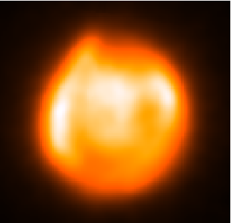
(a)

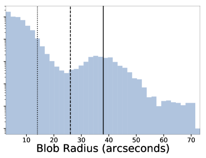
(b)

Figure 1: Left: Combined EPIC-pn and MOS exposure-corrected image in the 0.2-8.0 keV band. Right: EM-weighted blob radius histogram for the entire remnant, with the radius of the entire remnant (solid line), the central emission region (dashed line), and the width of outer shell (dotted line) also shown.

2 Methods

2.1 Separating Emission from Ejecta and Swept-Up Material

Frank . (2019) included maps showing the distribution of O, Ne, and Fe.The maps showed that O and Ne abundances are low throughout the entire remnant, while Fe is similarly low in the outer shell but significantly enhanced in the central emission region. The central region was therefore assumed to signify the ejected material from the explosion, which was isolated by selecting blobs with parameters kT $>1$ keV, Fe/Fe${}_{\odot}>$1. Here we apply the additional criterion that the blob radius be less than 26", the approximate radius of the central emission, see Figure 1. These larger blobs comprise only 3.5% of all the blobs and a small percentage of total emission measure (EM) of the kT $>1$ keV, Fe/Fe${}_{\odot}>$1 blobs. We have confirmed that the large blobs are unlikely to represent the central ejecta. However they have relatively large mass due to their large volumes, and thus disproportionately bias any mass estimates of the ejecta. All blobs not designated as ejecta are considered to be swept-up material. The total EM of the ejecta is EM = 8.82 ($\pm$ 2.31) $\times$ 10⁵⁷ cm^-3, and that of the swept-up material is 5.44 ($\pm$ 0.59) $\times$ 10⁵⁹ cm^-3.

2.2 Mass and Density

The density of a blob can be calculated from its emission measure and volume:

$$EM=\int{n_{e}n_{H}dV}$$ (1)

where $n_{e}$ is the electron density and $n_{H}$ is the hydrogen density. The EM is obtained directly from the vpshock model normalization. The blob radius, and thus volume (assumed to have a Gaussian profile), is a free parameter in the SPI fit, and can be computed for each blob. The mass can be derived from the density and the volume. However, equation 1 provides only the product of the electron and hydrogen densities. One more equation involving the two quantities is needed in order to obtain them individually. We consider three possible scenarios via which we can calculate these quantities. In each scenario, we assume that a blob has a uniform density, and the plasma is fully ionized. We have confirmed that assuming a partially ionized plasma does not appear to have a significant effect on our results, and any modifications generally lie within the error bars. The mass of each blob is derived individually, and summed over all blobs to determine the total mass.

The simplest scenario is to assume that all the emitting material consists of ‘typical’ LMC plasma, and to consider the EM and volume from the SPI fit. In this case, we use ‘typical’ abundances for the LMC as listed in Russell  Dopita (1992). This leads to an $n_{e}/n_{H}$ ratio of 1.087 and $\mu=0.602$ for each blob.

The second scenario allows for fit elements to deviate from the ‘typical’ LMC values. For those species thawed in the vpshock model, the abundance values are taken from the SPI fit, while the remaining species are assumed to have a ‘typical’ LMC abundance, as defined in Russell  Dopita (1992). Depending on the location of a blob, various different components, such as ejecta, swept-up medium or local LMC material, may contribute to the abundance value. Since each blob has a unique abundance value calculated from the SPI fit, it will have a unique value of $n_{e}/n_{H}$ and $\mu$. The mass of each blob is computed individually, and then they are all summed.

In these two scenarios, we calculate the mass of an individual element using the element’s mass fraction in the remnant. This fraction is calculated using the ratios $N_{i}/N_{ions}$, the number of atoms of a given element over the total number of atoms, and $m_{i}/\bar{m}$, the molecular weight of the element over the average ion mass. From this mass fraction and the total mass, the individual mass of a given element present in the plasma can be calculated.

The third scenario assumes the ejecta arise from a Type Ia explosion, where no hydrogen is present. It is therefore inappropriate to use the abundance returned by the SPI fit, because XSPEC assumes the presence of hydrogen. In order to compute the ejecta mass, we instead choose a Type Ia explosion model available in the literature, and use the given yields to specify the composition. Any Type Ia model that provides the mass yield per element can be used. The models we use are listed in Table 1. Given the yield of each element, and assuming it to be fully ionized, we can compute the number of free electrons, and the mean molecular weight $\mu$, in the same manner as the other scenarios. The main difference here is that we are assuming the composition is not defined by the SPI fit but by the Type Ia model. We note that we adopt the mass fraction of each element as given in a particular Type Ia model, but not the total mass predicted by the model. The total mass will be derived from the SPI volume and the density estimated. In some cases this may overestimate the mass. This may be because there is some swept-up material mixed in with the ejecta, but a large overestimate would generally mean that the assumption of a Ia is either untrue, or that even if it is true, the selected model is a poor approximation for the emitting gas.

3 Results and Discussion

3.1 Entire Remnant

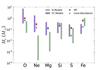
Figure 2: The mass of each element over the entire remnant, derived using the SPI measured abundances (red circle) and the Typical LMC scenario (blue triangle), in comparison with the range of values predicted by the core collapse (purple bar), and Type Ia (green bar) models listed in Table 1. All masses are in units of solar mass.

We first compare the total mass of each element for all the blobs with a selection of core collapse and Type Ia models. For each element, the mass is inferred from all the blobs using both the SPI measured abundance and the ‘typical LMC’ scenario. These are shown in Figure 2, alongside the range of masses predicted by both core collapse and Type Ia explosion models. The models considered are listed in Table 1. The measured masses of O, Ne, and Mg appear to correspond well with the core collapse models. However, these abundance values are also consistent with what would be expected from swept-up ambient LMC material. Although they seem a bit higher, this may be because the ‘typical LMC’ values in reality have considerable variation depending on position, latitude and the stellar environment, that is not accounted for. Alternatively, it is possible that these values may be fit by the typical LMC value with some contribution from the Type Ia material. Therefore the small enhancement of O, Ne, and Mg masses above the LMC value is not indicative of a core-collapse (CC) origin.

The predicted mass range for Si and S overlaps both the CC and Type Ia models, and has little discriminating power. The high measured Fe abundance, however, is totally inconsistent with an origin either in typical LMC material, or in core-collapse explosions. It can only be matched by the mass range predicted by Type Ia models. The Fe abundance therefore has the most discriminating power, and clearly suggests a Type Ia rather than a core-collapse SN explosion. In this we are consistent with previous authors, although with SPI we have the ability to determine abundances and other properties throughout the remnant as well as in any individual location.

Table 1: Supernova Explosion Models Used for Comparison.

Model Name	Group	Reference
N10	Ia DDT	S13
N100	Ia DDT	S13
N1600	Ia DDT	S13
N1600 0.5Z	Ia DDT	S13
050-1-c3-1	Ia DDT	L18
300-1-c3-1	Ia DDT	L18
500-1-c3-1	Ia DDT	L18
C-DEF	Ia DEF	M10
050-1-c3-1P	Ia DEF	L18
300-1-c3-1P	Ia DEF	L18
500-1-c3-1P	Ia DEF	L18
W18 s12.5	CC	S16
W18 s18.1	CC	S16
W18 s25.2	CC	S16
W18 s60.0	CC	S16
20M⊙ 10E51	CC	N06
40M⊙ 30E51	CC	N06
25A	CC	M03
25B	CC	M03
40A	CC	M03
40B	CC	M03

S13:Seitenzahl . (2013), L18:Leung  Nomoto (2018), M10:Maeda . (2010), S16:Sukhbold . (2016), N06:Nomoto . (2006), M03:Maeda  Nomoto (2003)

3.2 Swept-Up Material

The density histogram of the swept-up material is shown in Figure 3. The distribution results in an EM-weighted median density of $4.8\pm 1.1$ cm^-3. A map of the density is shown in Figure 4. The densities derived are found to be consistent with the densities from van der Heyden . (2003).

Figure 3: EM-weighted density histogram for the swept-up material, using the SPI measured abundances for the composition. The mode and median are shown as dashed and solid lines, respectively.

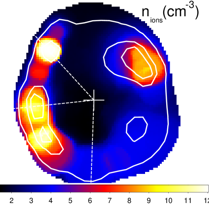
Figure 4: EM-weighted density map of the swept-up medium, with the density calculated using the SPI measured abundances. The white contours are from the overall EM map. The cross indicates the geometric center used to create the density profiles in Figure 5. Density is set to zero where the EM was lower than 0.05% of the mean to avoid noise due to poor statistics on the outer edges.

Using the density map, we plot the EM-weighted median density versus radius profile for three azimuthal positions (Figure 5). The selected position angles are shown in Figure 4 as white dashed lines. We clearly see high density blobs in the swept-up medium whose density far exceeds the ‘average’ density in the swept-up medium. The regions of highest density in Figure 4 appear to coincide with regions showing high H$\alpha$ emission (Rakowski ., 2009), thus further suggesting some form of density enhancement in this area.

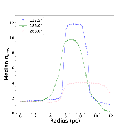
Figure 5: EM-weighted density as a function of radius for the swept-up material for three different position angles.

As described in Frank . (2019), numerical hydrodynamic simulations to compute the evolution of the remnant were carried out using the VH-1 code, a 3-dimensional numerical hydrodynamics code based on the Piecewise Parabolic Method Colella  Woodward (1984). The simulations were run in 2-dimensions. One quadrant was simulated, assuming spherical symmetry. As expected, the contact discontinuity between the inner and outer shocks is unstable to the Rayleigh-Taylor (R-T) instability, and R-T fingers are seen. Other than this there is nothing in the simulations that can break the spherical symmetry. Thus for the most part the swept-up medium in our simulation is quite uniform, as shown in Figure 6. The density shown in this figure is the number density, obtained simply by dividing the fluid density at each point by 1. $\times$ 10^-24, which may be considered as assuming a mean molecular weight $\approx$ 0.6, i.e. an assumption of complete ionization. On the other hand, the density map obtained from SPI (Figure 4), while also 2D, is in reality a 2D projection of a 3D environment where material may be mixed from the outset, and velocities in all directions may not necessarily be uniform. The dense regions in the outskirts of this map may be due to explosion inhomogeneities, an inhomogeneous surrounding medium, or mixing in turbulent layers during the explosion, none of which are captured in our simulations. Given this, it is comforting that the number densities from the simulations and those calculated by SPI are of the same order and differ by about a factor of 2 or so.

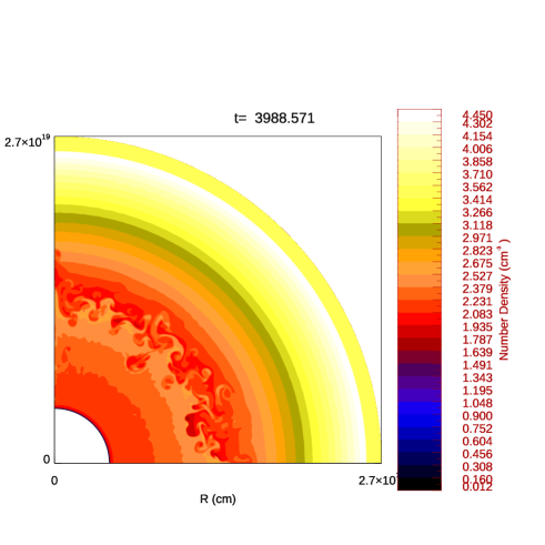
Figure 6: The number density of the plasma derived from our numerical simulations. The figure shows the density calculated by dividing the fluid density at each point by 1. $\times 10^{-24}$, which essentially assumes a fully ionized medium. In theory this may not be valid at all points, and the mean molecular weight may be different within the ejecta than the surrounding medium, but within the approximations this will suffice.

Since the swept-up material is assumed to have a ‘typical’ LMC abundance of hydrogen, the density and mass of the swept-up material can be computed as defined in Section 2.2. Using the measured SPI abundance to determine the composition, we find a total mass of the swept-up material of $228\pm 23$ M_⊙. This mass is much larger than that derived by van der Heyden . (2003). We suspect that this could be due to the volume of our surrounding medium, which exceeds the volume derived by van der Heyden . (2003). The latter used a spherical shell defined by somewhat arbitrary boundaries. In our case we isolated the ejecta as described above, and then computed the volume of each blob (assumed to have a Gaussian profile) and added it up to get the total volume. However we note also that we had some large volume blobs that we discarded as ejecta and are therefore now considered to be swept-up medium. Furthermore, the high density in the outer parts may be indicative of large density variations that were not considered by van der Heyden . (2003).

The mass of swept-up material can be independently estimated under the assumption that the SN expanded in a constant density medium, and that the supersonic shock wave swept up all the material in its path. In this case, assuming the density of the surrounding medium to be ${\rho}_{am}$, the swept up mass simply corresponds to $4\pi/3R_{sh}^{3}{\rho}_{am}$, where $R_{sh}$ is the radius of the outer shock. The latter is essentially the radius of the remnant. In our simulations we measured a shock radius of 8.5pc and a number density of 1.13 $\times 10^{-24}$ g cm^-3. This gives a mass of swept-up material of 42 M_⊙. Leahy (2017) calculated a radius of 9.45 pc and a density of 1.28, although they do not indicate what value of $\mu$ they use. For a value of 1, they would get about 110 M_⊙. A radius of 12 pc, close to the upper limit of suspected values, and closer to what we estimate from the data, would give a mass of 226 M_⊙ for the same value of $\mu$. Some of these values seem lower than SPI gives. However it is worth keeping in mind the high density blobs that we see in the outer regions, with number density approaching 12, much higher than even the shock densities. This may indicate significant density variations in the surrounding medium, thus invalidating the assumption of a constant density medium, and leading to the higher mass we find for the swept-up material.

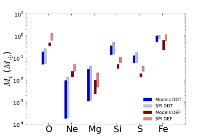
Figure 7: The mass yield (in solar masses) predicted by deflagration-to-detonation (DDT) (dark blue bar) and pure deflagration (dark red bar) Type Ia models, as listed in Table 1, in comparison with the ejecta mass calculated from the SPI results by assuming pure Type Ia ejecta composition using DDT (light blue bar) and deflagration (light red bar) models.

3.3 Ejecta Mass

To derive the ejecta mass, we use the pure Type Ia scenario outlined in Section 2.2, including only those blobs defined as ejecta. We calculate the mass using each and every one of the Type Ia models in Table 1. We consider the entire mass range from all models. The models are separated into two groups, those that consider a pure deflagration (i.e. a subsonic burning front), and those that incorporate a deflagration to detonation transition (i.e. a transition from a subsonic to a supersonic front). Our results are shown in Figure 7. The measured and predicted mass using the DDT models tend to agree very well, consistent with results in general for Type Ia’s. However, the deflagration models are not consistent with measurements.

4 Conclusions

In this paper we have expanded on our previous work on SNR DEM L71 (Frank ., 2019). We have better isolated the ejecta, computed the abundance of various elements and compared to detailed SN explosion models available in the literature. We have confirmed that DEM L71 shows an excess of Fe in the central region, which can only be produced within a Type Ia explosion, and is incompatible with a core-collapse explosion. Furthermore the abundance values are more compatible with DDT models than pure deflagration models. Our simulations are reasonably consistent with our extracted density map, although the map reveals inhomogeneities in the density distribution that cannot be captured in our simulations.

We are now applying our SPI technique to other SNRs observed with XMM-Newton, including W49B, and will show the results from these comparisons in future papers.

References

- Colella \BBA Woodward (\APACyear1984) \APACinsertmetastarcw84{APACrefauthors}Colella, P.\BCBT \BBA Woodward, P\BPBIR. \APACrefYearMonthDay1984\APACmonth09, \APACjournalVolNumPagesJournal of Computational Physics54174-201. {APACrefDOI} 10.1016/0021-9991(84)90143-8 \PrintBackRefs\CurrentBib
- Frank \BOthers. (\APACyear2019) \APACinsertmetastarfranketal19{APACrefauthors}Frank, K\BPBIA., Dwarkadas, V., Panfichi, A., Crum, R\BPBIM.\BCBL \BBA Burrows, D\BPBIN. \APACrefYearMonthDay2019\APACmonth04, \APACjournalVolNumPagesApJ87514. {APACrefDOI} 10.3847/1538-4357/ab0e81 \PrintBackRefs\CurrentBib
- Ghavamian \BOthers. (\APACyear2003) \APACinsertmetastarghavamianetal03{APACrefauthors}Ghavamian, P., Rakowski, C\BPBIE., Hughes, J\BPBIP.\BCBL \BBA Williams, T\BPBIB. \APACrefYearMonthDay2003Jun, \APACjournalVolNumPagesApJ5902833-845. {APACrefDOI} 10.1086/375161 \PrintBackRefs\CurrentBib
- Hughes \BOthers. (\APACyear2003) \APACinsertmetastarhughesetal03{APACrefauthors}Hughes, J\BPBIP., Ghavamian, P., Rakowski, C\BPBIE.\BCBL \BBA Slane, P\BPBIO. \APACrefYearMonthDay2003Jan, \APACjournalVolNumPagesApJ5822L95-L99. {APACrefDOI} 10.1086/367760 \PrintBackRefs\CurrentBib
- Leahy (\APACyear2017) \APACinsertmetastarLeahyetal17{APACrefauthors}Leahy, D\BPBIA. \APACrefYearMonthDay2017Mar, \APACjournalVolNumPagesApJ837136. {APACrefDOI} 10.3847/1538-4357/aa60c1 \PrintBackRefs\CurrentBib
- Leung \BBA Nomoto (\APACyear2018) \APACinsertmetastarln18{APACrefauthors}Leung, S\BHBIC.\BCBT \BBA Nomoto, K. \APACrefYearMonthDay2018Jul, \APACjournalVolNumPagesApJ8612143. {APACrefDOI} 10.3847/1538-4357/aac2df \PrintBackRefs\CurrentBib
- Maeda \BBA Nomoto (\APACyear2003) \APACinsertmetastarmn03{APACrefauthors}Maeda, K.\BCBT \BBA Nomoto, K. \APACrefYearMonthDay2003Dec, \APACjournalVolNumPagesApJ59821163-1200. {APACrefDOI} 10.1086/378948 \PrintBackRefs\CurrentBib
- Maeda \BOthers. (\APACyear2010) \APACinsertmetastarmaedaetal10{APACrefauthors}Maeda, K., Röpke, F\BPBIK., Fink, M., Hillebrandt, W., Travaglio, C.\BCBL \BBA Thielemann, F\BPBIK. \APACrefYearMonthDay2010Mar, \APACjournalVolNumPagesApJ7121624-638. {APACrefDOI} 10.1088/0004-637X/712/1/624 \PrintBackRefs\CurrentBib
- Nomoto \BOthers. (\APACyear2006) \APACinsertmetastarnomotoetal06{APACrefauthors}Nomoto, K., Tominaga, N., Umeda, H., Kobayashi, C.\BCBL \BBA Maeda, K. \APACrefYearMonthDay2006Oct, \APACjournalVolNumPagesNucl. Phys. A777424-458. {APACrefDOI} 10.1016/j.nuclphysa.2006.05.008 \PrintBackRefs\CurrentBib
- Peterson \BOthers. (\APACyear2007) \APACinsertmetastarspi{APACrefauthors}Peterson, J\BPBIR., Marshall, P\BPBIJ.\BCBL \BBA Andersson, K. \APACrefYearMonthDay2007Jan, \APACjournalVolNumPagesApJ6551109-127. {APACrefDOI} 10.1086/509095 \PrintBackRefs\CurrentBib
- Rakowski \BOthers. (\APACyear2003) \APACinsertmetastarrakowskietal03{APACrefauthors}Rakowski, C\BPBIE., Ghavamian, P.\BCBL \BBA Hughes, J\BPBIP. \APACrefYearMonthDay2003Jun, \APACjournalVolNumPagesApJ5902846-857. {APACrefDOI} 10.1086/375162 \PrintBackRefs\CurrentBib
- Rakowski \BOthers. (\APACyear2009) \APACinsertmetastarR09{APACrefauthors}Rakowski, C\BPBIE., Ghavamian, P.\BCBL \BBA Laming, J\BPBIM. \APACrefYearMonthDay2009May, \APACjournalVolNumPagesApJ69622195-2205. {APACrefDOI} 10.1088/0004-637X/696/2/2195 \PrintBackRefs\CurrentBib
- Russell \BBA Dopita (\APACyear1992) \APACinsertmetastarrd92{APACrefauthors}Russell, S\BPBIC.\BCBT \BBA Dopita, M\BPBIA. \APACrefYearMonthDay1992Jan, \APACjournalVolNumPagesApJ384508. {APACrefDOI} 10.1086/170893 \PrintBackRefs\CurrentBib
- Seitenzahl \BOthers. (\APACyear2013) \APACinsertmetastarseitenzahletal13{APACrefauthors}Seitenzahl, I\BPBIR., Ciaraldi-Schoolmann, F., Röpke, F\BPBIK. et al. \APACrefYearMonthDay2013Feb, \APACjournalVolNumPagesMNRAS42921156-1172. {APACrefDOI} 10.1093/mnras/sts402 \PrintBackRefs\CurrentBib
- Sukhbold \BOthers. (\APACyear2016) \APACinsertmetastarsukhboldetal16{APACrefauthors}Sukhbold, T., Ertl, T., Woosley, S\BPBIE., Brown, J\BPBIM.\BCBL \BBA Janka, H\BPBIT. \APACrefYearMonthDay2016Apr, \APACjournalVolNumPagesApJ821138. {APACrefDOI} 10.3847/0004-637X/821/1/38 \PrintBackRefs\CurrentBib
- van der Heyden \BOthers. (\APACyear2003) \APACinsertmetastarvanderheydenetal03{APACrefauthors}van der Heyden, K\BPBIJ., Bleeker, J\BPBIA\BPBIM., Kaastra, J\BPBIS.\BCBL \BBA Vink, J. \APACrefYearMonthDay2003\APACmonth07, \APACjournalVolNumPagesA&A406141-148. {APACrefDOI} 10.1051/0004-6361:20030658 \PrintBackRefs\CurrentBib