Abstract

Regret analysis is challenging in Multi-Agent Reinforcement Learning (MARL) primarily due to the dynamical environments and the decentralized information among agents. We attempt to solve this challenge in the context of decentralized learning in multi-agent linear-quadratic (LQ) dynamical systems. We begin with a simple setup consisting of two agents and two dynamically decoupled stochastic linear systems, each system controlled by an agent. The systems are coupled through a quadratic cost function. When both systems’ dynamics are unknown and there is no communication among the agents, we show that no learning policy can generate sub-linear in $T$ regret, where $T$ is the time horizon. When only one system’s dynamics are unknown and there is one-directional communication from the agent controlling the unknown system to the other agent, we propose a MARL algorithm based on the construction of an auxiliary single-agent LQ problem. The auxiliary single-agent problem in the proposed MARL algorithm serves as an implicit coordination mechanism among the two learning agents. This allows the agents to achieve a regret within $O(\sqrt{T})$ of the regret of the auxiliary single-agent problem. Consequently, using existing results for single-agent LQ regret, our algorithm provides a $\tilde{O}(\sqrt{T})$ regret bound. (Here $\tilde{O}(\cdot)$ hides constants and logarithmic factors). Our numerical experiments indicate that this bound is matched in practice. From the two-agent problem, we extend our results to multi-agent LQ systems with certain communication patterns.

1 Introduction

Multi-agent systems arise in many different domains, including multi-player card games (Bard et al.,, 2019), robot teams (Stone and Veloso,, 1998), vehicle formations (Fax and Murray,, 2004), urban traffic control (De Oliveira and Camponogara,, 2010), and power grid operations (Schneider et al.,, 1999). A multi-agent system consists of multiple autonomous agents operating in a common environment. Each agent gets observations from the environment (and possibly from some other agents) and, based on these observations, each agent chooses actions to collect rewards from the environment. The agents’ actions may influence the environment dynamics and the reward of each agent. Multi-agent systems where the environment model is known to all agents have been considered under the frameworks of multi-agent planning (Oliehoek et al.,, 2016), decentralized optimal control (Yüksel and Başar,, 2013), and non-cooperative game theory (Basar and Olsder,, 1999). In realistic situations, however, the environment model is usually only partially known or even totally unknown. Multi-Agent Reinforcement Learning (MARL) aims to tackle the general situation of multi-agent sequential decision-making where the environment model is not completely known to the agents. In the absence of the environmental model, each agent needs to learn the environment while interacting with it to collect rewards. In this work, we focus on decentralized learning in a cooperative multi-agent setting where all agents share the same reward (or cost) function.

A number of successful learning algorithms have been developed for Single-Agent Reinforcement Learning (SARL) in single-agent environment models such as finite Markov decision processes (MDPs) and linear quadratic (LQ) dynamical systems. To extend SARL algorithms to cooperative MARL problems, one key challenge is the coordination among agents (Panait and Luke,, 2005; Hernandez-Leal et al.,, 2017). In general, agents have access to different information and hence agents may have different views about the environment from their different learning processes. This difference in perspectives makes it difficult for agents to coordinate their actions for maximizing rewards.

One popular method to resolve the coordination issue is to have a central entity collect information from all agents and determine the policies for each agent. Several works generalize SARL methods to multi-agent settings with such an approach by either assuming the existence of a central controller or by training a centralized agent with information from all agents in the learning process, which is the idea of centralized training with decentralized execution (Foerster et al.,, 2016; Dibangoye and Buffet,, 2018; Hernandez-Leal et al.,, 2018). With centralized information, the learning problem reduces to a single-agent problem which can be readily solved by SARL algorithms. In many real-world scenarios, however, there does not exist a central controller or a centralized agent receiving all the information. Agents have to learn in a decentralized manner based on the observations they get from the environment and possibly from some other agents. In the absence of a centralized entity, an efficient MARL algorithm should guide each agent to learn the environment while maintaining certain level of coordination among agents.

Moreover, in online learning scenarios, the trade-off between exploration and exploitation is critical for the performance of a MARL algorithm during learning (Hernandez-Leal et al.,, 2017). Most existing SARL algorithms balance the exploration-exploitation trade off by controlling the posterior estimates/beliefs of the agent. Since multiple agents have decentralized information in MARL, it is not possible to directly extend SARL methods given the agents’ distinct posterior estimates/beliefs. Furthermore, the fact that each agent’s estimates/beliefs may be private to itself prevents any direct imitation of SARL. These issues make it extremely challenging to design coordinated policies for multiple agents to learn the environment and maintain good performance during learning. In this work, we attempt to solve this challenge in online decentralized MARL in the context of multi-agent learning in linear-quadratic (LQ) dynamical systems. Learning in LQ systems is an ideal benchmark for studying MARL due to a combination of its theoretical tractability and its practical application in various engineering domains (Aström and Murray,, 2010; Abbeel et al.,, 2007; Levine et al.,, 2016; Abeille et al.,, 2016; Lazic et al.,, 2018).

We begin with a simple setup consisting of two agents and two stochastic linear systems as shown in Figure 1. The systems are dynamically decoupled but coupled through a quadratic cost function. In spite of its simplicity, this setting illustrates some of the inherent challenges and potential results in MARL. When the parameters of both systems 1 and 2 are known to both agents, the optimal solution to this multi-agent control problem can be computed in closed form (Ouyang et al.,, 2018). We consider the settings where the system parameters are completely or partially unknown and formulate an online MARL problem to minimize the agents’ regret during learning. The regret is defined to be the difference between the cost incurred by the learning agents and the steady-state cost of the optimal policy computed using complete knowledge of the system parameters.

We provide a finite-time regret analysis for a decentralized MARL problem with controlled dynamical systems. In particular, we show that

1. First, if all parameters of a system are unknown, then both agents should receive information about the state of this system; otherwise, there is no learning policy that can guarantee sub-linear regret for all instances of the decentralized MARL problem (Theorem 1 and Lemma 2).

2. Further, when only one system’s dynamics are unknown and there is one-directional communication from the agent controlling the unknown system to the other agent, we propose a MARL algorithm with regret bounded by $\tilde{O}(\sqrt{T})$ (Theorem 2 and Corollary 1).

The proposed MARL algorithm builds on an auxiliary SARL problem constructed from the MARL problem. Each agent constructs the auxiliary SARL problem by itself and applies a SARL algorithm $\mathcal{A}$ to it. Each agent chooses its action by modifying the output of the SARL algorithm $\mathcal{A}$ based on its information at each time. In our proposed algorithm, the auxiliary SARL problem serves as the critical coordination tool for the two agents to learn individually while jointly maintaining an exploration-exploitation balance. In fact, we will later show that the SARL dynamics can be seen as the filtering equation for the common state estimate of the agents.

We show that the regret achieved by our MARL algorithm is upper bounded by the regret of the SARL algorithm $\mathcal{A}$ in the auxiliary SARL problem plus an overhead bounded by $O(\sqrt{T})$. This implies that the MARL regret can be bounded by $\tilde{O}(\sqrt{T})$ by letting $\mathcal{A}$ be one of the state-of-the-art SARL algorithms for LQ systems which achieve $\tilde{O}(\sqrt{T})$ regret (Abbasi-Yadkori and Szepesvári,, 2011; Ibrahimi et al.,, 2012; Faradonbeh et al.,, 2017, 2019). Our numerical experiments indicate that this bound is matched in simulations. From the two-agent problem, we extend our results to multi-agent LQ systems with certain communication patterns.

Related work. There exists a rich and expanding body of work in the field of MARL (Littman,, 1994; Bu et al.,, 2008; Nowé et al.,, 2012). Despite recent successes in empirical works including the adaptation of deep learning (Hernandez-Leal et al.,, 2018), many theoretical aspects of MARL are still under-explored. As multiple agents learn and adapt their policies, the environment is non-stationary from a single agent’s perspective (Hernandez-Leal et al.,, 2017). Therefore, convergence guarantees of SARL algorithms are mostly invalid for MARL problems. Several works have extended SARL algorithms to independent or cooperative agents and analyzed their convergence properties (Tan,, 1993; Greenwald et al.,, 2003; Matignon and Fort-Piat,, 2012; Kar et al.,, 2013; Amato and Oliehoek,, 2015; Zhang et al.,, 2018; Gagrani and Nayyar,, 2018; Wai et al.,, 2018). However, most of these works do not take into account the performance during learning except Bowling, (2005). The algorithm of Bowling, (2005) has a regret bound of $O(\sqrt{T})$, but the analysis is limited to repeated games. In contrast, we are interested in MARL in dynamical systems.

Regret analysis in online learning has been mostly focusing on multi-armed bandit (MAB) problems (Lai and Robbins,, 1985). Upper-Confidence-Bound (UCB) (Auer and Fischer,, 2002; Bubeck and Cesa-Bianchi,, 2012; Dani et al.,, 2008) and Thompson Sampling (Thompson,, 1933; Kaufmann et al.,, 2012; Agrawal and Goyal,, 2013; Russo and Van Roy,, 2014) are the two popular classes of algorithms that provide near-optimal regret guarantees in single-agent MAB. These ideas have been extended to certain multi-agent MAB settings (Liu and Zhao,, 2010; Korda and Shuai,, 2016; Nayyar and Jain,, 2016). Multi-agent MAB can be viewed as a special class of MARL problems, but the lack of dynamics in MAB environments makes a drastic difference from the dynamical setting in this paper.

In the learning of dynamical systems, recent works have adopted concepts from MAB to analyze the regret of SARL algorithms in MDP (Jaksch et al.,, 2010; Osband et al.,, 2013; Gopalan and Mannor,, 2015; Ouyang et al., 2017b, ) and LQ systems (Abbasi-Yadkori and Szepesvári,, 2011; Ibrahimi et al.,, 2012; Faradonbeh et al.,, 2017, 2019; Ouyang et al., 2017a, ; Faradonbeh et al.,, 2018; Abbasi-Yadkori and Szepesvári,, 2015; Abeille and Lazaric,, 2018). Our MARL algorithm builds on these SARL algorithms by using the novel idea of constructing an auxiliary SARL problem for multi-agent coordination.

Figure 1: Two-agent system model. Solid lines indicate communication links, dashed lines indicate control links, and dotted lines indicate the possibility of information sharing.

Notation. The collection of matrices $A^{1}$ and $A^{2}$ (resp. vectors $x^{1}$ and $x^{2}$) is denoted as $A^{1,2}$ (resp. $x^{1,2}$). Given column vectors $x^{1}$ and $x^{2}$, the notation $\operatorname{\mathbf{vec}}(x^{1},x^{2})$ is used to denote the column vector formed by stacking $x^{1}$ on top of $x^{2}$. We use $[P^{\cdot,\cdot}]_{1,2}$ and $\textbf{diag}(P^{1},P^{2})$ to denote the following block matrices, $[P^{\cdot,\cdot}]_{1,2}:=\begin{bmatrix}P^{11}&P^{12}\\ P^{21}&P^{22}\end{bmatrix}$, $\textbf{diag}(P^{1},P^{2})=\begin{bmatrix}P^{1}&\mathbf{0}\\ \mathbf{0}&P^{2}\end{bmatrix}$.

2 Problem Formulation

Consider a multi-agent Linear-Quadratic (LQ) system consisting of two systems and two associated agents as shown in Figure 1. The linear dynamics of systems 1 and 2 are given by

$$x_{t+1}^{1} =A_{*}^{1}x_{t}^{1}+B_{*}^{1}u_{t}^{1}+w_{t}^{1},$$

$$x_{t+1}^{2} =A_{*}^{2}x_{t}^{2}+B_{*}^{2}u_{t}^{2}+w_{t}^{2},$$ (1)

where for $n\in\{1,2\}$, $x_{t}^{n}\in\mathbb{R}^{d_{x}^{n}}$ is the state of system $n$ and $u_{t}^{n}\in\mathbb{R}^{d_{u}^{n}}$ is the action of agent $n$. $A_{*}^{1,2}$ and $B_{*}^{1,2}$ are system matrices with appropriate dimensions. We assume that for $n\in\{1,2\}$, $w_{t}^{n}$, $t\geq 0$, are i.i.d with standard Gaussian distribution $\mathcal{N}(\mathbf{0},\mathbf{I})$. The initial states $x_{0}^{1,2}$ are assumed to be fixed and known.

The overall system dynamics can be written as,

$$x_{t+1}=A_{*}x_{t}+B_{*}u_{t}+w_{t},$$ (2)

where we have defined $x_{t}=\operatorname{\mathbf{vec}}(x_{t}^{1},x_{t}^{2}),u_{t}=\operatorname{\mathbf{vec}}(u_{t}^{1},u_{t}^{2}),w_{t}=\operatorname{\mathbf{vec}}(w_{t}^{1},w_{t}^{2})$, $A_{*}=\textbf{diag}(A_{*}^{1},A_{*}^{2})$, and $B_{*}=\textbf{diag}(B_{*}^{1},B_{*}^{2})$.

At each time $t$, agent $n$, $n\in\{1,2\}$, perfectly observes the state $x_{t}^{n}$ of its respective system. The pattern of information sharing plays an important role in the analysis of multi-agent systems. In order to capture different information sharing patterns between the agents, let $\gamma^{n}\in\{0,1\}$ be a fixed binary variable indicating the availability of a communication link from agent $n$ to the other agent. Then, $i_{t}^{n}$ which is the information sent by agent $n$ to the other agent can be written as,

$$i_{t}^{n}=\begin{cases}x_{t}^{n}&\quad\text{if }\gamma^{n}=1\\ \varnothing&\quad\text{otherwise}\end{cases}.$$ (3)

At each time $t$, agent $n$’s action is a function $\pi_{t}^{n}$ of its information $h_{t}^{n}$, that is, $u_{t}^{n}=\pi_{t}^{n}(h_{t}^{n})$ where $h_{t}^{1}=\{x_{0:t}^{1},u_{0:t-1}^{1},i_{0:t}^{2}\}$ and $h_{t}^{2}=\{x_{0:t}^{2},u_{0:t-1}^{2},i_{0:t}^{1}\}$. Let $\pi=(\pi^{1},\pi^{2})$ where $\pi^{n}=(\pi_{0}^{n},\pi_{1}^{n},\ldots)$. We will look at two following information sharing patterns:

1. No information sharing ($\gamma^{1}=\gamma^{2}=0$),

2. One-way information sharing from agent 1 to agent 2 ($\gamma^{1}=1$, $\gamma^{2}=0$).

At time $t$, the system incurs an instantaneous cost $c(x_{t},u_{t})$, which is a quadratic function given by

$$c(x_{t},u_{t}) =x_{t}^{\intercal}Qx_{t}+u_{t}^{\intercal}Ru_{t},$$ (4)

where $Q=[Q^{\cdot,\cdot}]_{1,2}$ is a known symmetric positive semi-definite (PSD) matrix and $R=[R^{\cdot,\cdot}]_{1,2}$ is a known symmetric positive definite (PD) matrix.

2.1 The optimal multi-agent linear-quadratic problem

Let $\theta_{*}^{n}=[A_{*}^{n},B_{*}^{n}]$ be the dynamics parameter of system $n$, $n\in\{1,2\}$. When $\theta_{*}^{1}$ and $\theta_{*}^{2}$ are perfectly known to the agents, minimizing the infinite horizon average cost is a multi-agent stochastic Linear Quadratic (LQ) control problem. Let $J(\theta_{*}^{1,2})$ be the optimal infinite horizon average cost under $\theta_{*}^{1,2}$, that is,

$$J(\theta_{*}^{1,2})=\inf_{\pi}\limsup_{T\rightarrow\infty}\frac{1}{T}\sum_{t=0}^{T-1}\operatorname{\mathbb{E}}^{\pi}[c(x_{t},u_{t})|\theta_{*}^{1,2}].$$ (5)

We make the following standard assumption about the multi-agent stochastic LQ problem.

Assumption 1.

$(A_{*},B_{*})$ is stabilizable and $(A_{*},Q^{1/2})$ is detectable.

The above decentralized stochastic LQ problem has been studied by Ouyang et al., (2018). The following lemma summarizes this result.

Lemma 1 (Ouyang et al., (2018)).

Under Assumption 1, the optimal control strategies are given by

$$u^{1}_{t} =K^{1}(\theta_{*}^{1,2})\begin{bmatrix}\hat{x}_{t}^{1}\\ \hat{x}_{t}^{2}\end{bmatrix}+\tilde{K}^{1}(\theta_{*}^{1})(x_{t}^{1}-\hat{x}_{t}^{1}),$$

$$u^{2}_{t} =K^{2}(\theta_{*}^{1,2})\begin{bmatrix}\hat{x}_{t}^{1}\\ \hat{x}_{t}^{2}\end{bmatrix}+\tilde{K}^{2}(\theta_{*}^{2})(x_{t}^{2}-\hat{x}_{t}^{2}),$$ (6)

where the gain matrices $K^{1}(\theta_{*}^{1,2}),K^{2}(\theta_{*}^{1,2}),\tilde{K}^{1}(\theta_{*}^{1})$, and $\tilde{K}^{2}(\theta_{*}^{2})$ can be computed offline and $\hat{x}_{t}^{n}$, $n\in\{1,2\}$, can be computed recursively according to

$$\hat{x}_{0}^{n}=x_{0}^{n},\quad\hat{x}_{t+1}^{n}=$$

$$\begin{cases}x_{t+1}^{n}&\text{if }\gamma^{n}=1\\ A_{*}^{n}\hat{x}_{t}^{n}+B_{*}^{n}K^{n}(\theta_{*}^{1,2})\operatorname{\mathbf{vec}}(\hat{x}_{t}^{1},\hat{x}_{t}^{2})&\text{otherwise}\end{cases}.$$ (7)

2.2 The multi-agent reinforcement learning problem

The problem we are interested in is to minimize the infinite horizon average cost when the matrices $A_{*}$ and $B_{*}$ of the system are unknown. In this case, the control problem described by (1)-(4) can be seen as a Multi-Agent Reinforcement Learning (MARL) problem where both agents need to learn the system parameters $\theta_{*}^{1}=[A_{*}^{1},B_{*}^{1}]$ and $\theta_{*}^{2}=[A_{*}^{2},B_{*}^{2}]$ in order to minimize the infinite horizon average cost. The learning performance of policy $\pi$ is measured by the cumulative regret over $T$ steps defined as,

$$R(T,\pi)=\sum_{t=0}^{T-1}\left[c(x_{t},u_{t})-J(\theta_{*}^{1,2})\right],$$ (8)

which is the difference between the performance of the agents under policy $\pi$ and the optimal infinite horizon cost under full information about the system dynamics. Thus, the regret can be interpreted as a measure of the cost of not knowing the system dynamics.

3 An Auxiliary Single-Agent LQ Problem

In this section, we construct an auxiliary single-agent LQ control problem based on the MARL problem of Section 2. This auxiliary single-agent LQ control problem is inspired by the common information based coordinator (which has been developed in non-learning settings in Nayyar et al., (2013) and Asghari et al., (2018) and the references therein). We will later use the auxiliary problem as a coordination mechanism for our MARL algorithm.

Consider a single-agent system with dynamics

$$x_{t+1}^{\diamond}=A_{*}x_{t}^{\diamond}+B_{*}u_{t}^{\diamond}+\begin{bmatrix}w_{t}^{1}\\ \mathbf{0}\end{bmatrix},$$ (9)

where $x_{t}^{\diamond}\in\mathbb{R}^{d_{x}^{1}+d_{x}^{2}}$ is the state of the system, $u_{t}^{\diamond}\in\mathbb{R}^{d_{u}^{1}+d_{u}^{2}}$ is the action of the auxiliary agent, $w_{t}^{1}$ is the noise vector of system 1 defined in (1), and matrices $A_{*}$ and $B_{*}$ are as defined in (2). The initial state $x_{0}^{\diamond}$ is assumed to be equal to $x_{0}$. The action $u_{t}^{\diamond}=\pi_{t}^{\diamond}(h_{t}^{\diamond})$ at time $t$ is a function of the history of observations $h_{t}^{\diamond}=\{x_{0:t}^{\diamond},u_{0:t-1}^{\diamond}\}$. The auxiliary agent’s strategy is denoted by $\pi^{\diamond}=(\pi_{1}^{\diamond},\pi_{2}^{\diamond},\ldots)$. The instantaneous cost $c(x_{t}^{\diamond},u_{t}^{\diamond})$ of the system is a quadratic function given by

$$c(x_{t}^{\diamond},u_{t}^{\diamond}) =(x_{t}^{\diamond})^{\intercal}Qx_{t}^{\diamond}+(u_{t}^{\diamond})^{\intercal}Ru_{t}^{\diamond},$$ (10)

where matrices $Q$ and $R$ are as defined in (4).

When the parameters $\theta_{*}^{1}$ and $\theta_{*}^{2}$ are unknown, we will have a Single-Agent Reinforcement Learning (SARL) problem. In this problem, the regret of a policy $\pi^{\diamond}$ over $T$ steps is given by

$$R^{\diamond}(T,\pi^{\diamond})=\sum_{t=0}^{T-1}\left[c(x_{t}^{\diamond},u_{t}^{\diamond})-J^{\diamond}(\theta_{*}^{1,2})\right],$$ (11)

where $J^{\diamond}(\theta_{*}^{1,2})$ is the optimal infinite horizon average cost under $\theta_{*}^{1,2}$.

Existing algorithms for the SARL problem are generally based on the two following approaches: Optimism in the Face of Uncertainty (OFU) (Abbasi-Yadkori and Szepesvári,, 2011; Ibrahimi et al.,, 2012; Faradonbeh et al.,, 2017, 2019) and Thompson Sampling (TS) (also known as posterior sampling) (Faradonbeh et al.,, 2017; Abbasi-Yadkori and Szepesvári,, 2015; Abeille and Lazaric,, 2018). In spite of the differences among these algorithms, all can be generally described as the AL-SARL algorithm (algorithm for the SARL problem). In this algorithm, at each time $t$, the agent interacts with a SARL learner (see Appendix I for a detailed description the SARL learner) by feeding time $t$ and the state $x_{t}^{\diamond}$ to it and receiving estimates $\theta_{t}^{1}=[A_{t}^{1},B_{t}^{1}]$ and $\theta_{t}^{2}=[A_{t}^{2},B_{t}^{2}]$ of the unknown parameters $\theta_{*}^{1,2}$. Then, the agent uses $\theta_{t}^{1,2}$ to calculate the gain matrix $K(\theta_{t}^{1,2})$ (see Appendix J for a detailed description of this matrix) and executes the action $u_{t}^{\diamond}=K(\theta_{t}^{1,2})x_{t}^{\diamond}$. As a result, a new state $x_{t+1}^{\diamond}$ is observed.

Among the existing algorithms, OFU-based algorithms of Abbasi-Yadkori and Szepesvári, (2011); Ibrahimi et al., (2012); Faradonbeh et al., (2017, 2019) and the TS-based algorithm of Faradonbeh et al., (2017) achieve a $\tilde{O}(\sqrt{T})$ regret for the SARL problem (Here $\tilde{O}(\cdot)$ hides constants and logarithmic factors).

Algorithm 1 AL-SARL

Initialize $\mathcal{L}$ and $x_{0}^{\diamond}$

for $t=0,1,\ldots$ do

     Feed time $t$ and state $x_{t}^{\diamond}$ to $\mathcal{L}$ and get $\theta_{t}^{1}$ and $\theta_{t}^{2}$

     Compute $K(\theta_{t}^{1,2})$

     Execute $u_{t}^{\diamond}=K(\theta_{t}^{1,2})x_{t}^{\diamond}$

     Observe new state $x_{t+1}^{\diamond}$

end for

4 Main Results

In this section, we start with the regret analysis for the case where the parameters of both systems are unknown (that is, $\theta_{*}^{1}$ and $\theta_{*}^{2}$ are unknown) and there is no information sharing between the agents (that is, $\gamma^{1}=\gamma^{2}=0$). The detailed proofs for all results are in the appendix.

4.1 Unknown $\theta_{*}^{1}$ and $\theta_{*}^{2}$, no information sharing ($\gamma^{1}=\gamma^{2}=0$)

For the MARL problem of this section (it is called MARL1 for future reference), we show that there is no learning algorithm with a sub-linear in $T$ regret for all instances of the MARL1 problem. The following theorem states this result.

Theorem 1.

There is no algorithm that can achieve a lower-bound better than $\Omega(T)$ on the regret of all instances of the MARL1 problem.

A $\Omega(T)$ regret implies that the average performance of the learning algorithm has at least a constant gap from the ideal performance of informed agents. This prevent efficient learning performance even in the limit. Theorem 1 implies that in a MARL1 problem where the system dynamics are unknown, learning is not possible without communication between the agents. The proof of Theorem 1 also provides the following result.

Lemma 2.

Consider a MARL problem where the parameter of system 2 (that is, $\theta_{*}^{2}$) is known to both agents and only the parameter of system 1 (that is, $\theta_{*}^{1}$) is unknown. Further, there is no communication between the agents. Then, there is no algorithm that can achieve a lower-bound better than $\Omega(T)$ on the regret of all instances of this MARL problem.

The above results imply that if the parameter of a system is unknown, both agents should receive information about this unknown system; otherwise, there is no learning policy $\pi$ that can guarantee a sub-linear in $T$ regret for all instances of this MARL problem.

In the next section, we assume that $\theta_{*}^{2}$ is known to both agents and only $\theta_{*}^{1}$ is unknown. Further, we assume the presence of a communication link from agent 1 to agent 2, that is, $\gamma^{1}=1$. This communication link allows agent 2 to receive feedback about the state $x_{t}^{1}$ of system 1 and hence, remedies the impossibility of learning for agent 2.

4.2 Unknown $\theta_{*}^{1}$, one-way information sharing from agent 1 to agent 2 ($\gamma^{1}=1$, $\gamma^{2}=0$)

In this section, we consider the case where only system 1 is unknown and there is one-way communication from agent 1 to agent 2. Despite this one-way information sharing, the two agents still have different information. In particular, at each time agent 2 observes the state $x^{2}_{t}$ of system 2 which is not available to agent 1. For the MARL of this section (it is called MARL2 for future reference), we propose the AL-MARL algorithm which builds on the auxiliary SARL problem of Section 3. AL-MARL algorithm is a decentralized multi-agent algorithm which is performed independently by the agents. Every agent independently constructs an auxiliary SARL problem where $x_{t}^{\diamond}=\operatorname{\mathbf{vec}}(x_{t}^{1},\check{x}_{t}^{2})$ and applies an AL-SARL algorithm with its own learner $\mathcal{L}$ to it in order to learn the unknown parameter $\theta_{*}^{1}$ of system 1. In this algorithm, $\check{x}_{t}^{2}$ (described in the AL-MARL algorithm) is a proxy for $\hat{x}_{t}^{2}$ of (7) updated using the estimate $\theta_{t}^{1}$ instead of the unknown parameter $\theta_{*}^{1}$.

At time $t$, each agent feeds $\operatorname{\mathbf{vec}}(x_{t}^{1},\check{x}_{t}^{2})$ to its own SARL learner $\mathcal{L}$ and gets $\theta_{t}^{1}$ and $\theta_{t}^{2}$. Note that both agents already know the true parameter $\theta_{*}^{2}$, hence they only use $\theta_{t}^{1}$ to compute their gain matrix $K^{\texttt{agent_ID}}(\theta_{t}^{1},\theta_{*}^{2})$ and use this gain matrix to compute their actions $u_{t}^{1}$ and $u_{t}^{2}$ according to the AL-MARL algorithm. Note that agent 2 needs $\tilde{K}^{2}(\theta_{*}^{2})$ to calculate its actions $u_{t}^{2}$. However, we know that $\tilde{K}^{2}(\theta_{*}^{2})$ is independent of the unknown parameter $\theta_{*}^{1}$ and hence, $\tilde{K}^{2}(\theta_{*}^{2})$ can be calculated prior to the beginning of the algorithm. After the execution of the actions $u_{t}^{1}$ and $u_{t}^{2}$ by the agents, both agents observe the new state $x_{t+1}^{1}$ and agent 2 further observes the new state $x_{t+1}^{2}$. Finally, each agent independently computes $\check{x}_{t+1}^{2}$.

Remark 1.

The state $x_{t}^{\diamond}$ of the auxiliary SARL can be interpreted as an estimate of the state $x_{t}$ of the overall system (2) that each agent computes based on the common information between them. In fact, the SARL dynamics in (9) can be seen as the filtering equation for this common estimate.

Remark 2.

We want to emphasize that unlike the idea of centralized training with decentralized execution (Foerster et al.,, 2016; Dibangoye and Buffet,, 2018; Hernandez-Leal et al.,, 2018), the AL-MARL algorithm is an online decentralized learning algorithm. This means that there is no centralized learning phase in the setup where agents can collect information or have access to a simulator. The agents are simultaneously learning and controlling the system.

Remark 3.

Since the SARL learner $\mathcal{L}$ can include taking samples and solving optimization problems, due to the independent execution of the AL-MARL algorithm, agents might receive different $\theta_{t}^{1,2}$ from their own learner $\mathcal{L}$.

In order to avoid the issue pointed out in Remark 3, we make an assumption about the output of the SARL learner $\mathcal{L}$.

Assumption 2.

Given the same time and same state input to the SARL learner $\mathcal{L}$, the outputs $\theta_{t}^{1,2}$ from different learners $\mathcal{L}$ are the same.

Note that Assumption 2 can be easily achieved by setting the same initial sampling seed (if the SARL learner $\mathcal{L}$ includes taking samples) or by setting the same tie-breaking rule among possible similar solutions of an optimization problem (if the SARL learner $\mathcal{L}$ include solving optimization problems). Now, we present the following result which is based on Assumption 2.

Theorem 2.

Under Assumption 2, let $R(T,\texttt{AL-MARL})$ be the regret for the MARL2 problem under the policy of the AL-MARL algorithm and $R^{\diamond}(T,\texttt{AL-SARL})$ be the regret for the auxiliary SARL problem under the policy of the AL-SARL algorithm. Then for any $\delta\in(0,1/e)$, with probability at least $1-\delta$,

$$R(T,\texttt{AL-MARL})\leq R^{\diamond}(T,\texttt{AL-SARL})+\log(\frac{1}{\delta})\tilde{K}\sqrt{T}.$$ (12)

Algorithm 2 AL-MARL

Input: agent_ID, learner $\mathcal{L}$, $x_{0}^{1}$, and $x_{0}^{2}$

Initialize $\mathcal{L}$ and $\check{x}_{0}^{2}=x_{0}^{2}$

for $t=0,1,\ldots$ do

     Feed time $t$ and state $\operatorname{\mathbf{vec}}(x_{t}^{1},\check{x}_{t}^{2})$ to $\mathcal{L}$ and

        get $\theta_{t}^{1}=[A_{t}^{1},B_{t}^{1}]$ and $\theta_{t}^{2}=[A_{t}^{2},B_{t}^{2}]$

     Compute $K^{\texttt{agent_ID}}(\theta_{t}^{1},\theta_{*}^{2})$

     if $\texttt{agent_ID}=1$ then

         Execute $u_{t}^{1}=K^{1}(\theta_{t}^{1},\theta_{*}^{2})\operatorname{\mathbf{vec}}(x_{t}^{1},\check{x}_{t}^{2})$

     else

         Execute $u_{t}^{2}=K^{2}(\theta_{t}^{1},\theta_{*}^{2})\operatorname{\mathbf{vec}}(x_{t}^{1},\check{x}_{t}^{2})$

                          $+\tilde{K}^{2}(\theta_{*}^{2})(x_{t}^{2}-\check{x}_{t}^{2})$

     end if

     Observe new state $x_{t+1}^{1}$

     Compute $\check{x}_{t+1}^{2}=A_{*}^{2}\check{x}_{t}^{2}$

                         $+B_{*}^{2}K^{2}(\theta_{t}^{1},\theta_{*}^{2})\operatorname{\mathbf{vec}}(x_{t}^{1},\check{x}_{t}^{2})$

     if $\texttt{agent_ID}=2$ then

         Observe new state $x_{t+1}^{2}$

     end if

end for

This result shows that under the policy of the AL-MARL algorithm, the regret for the MARL2 problem is upper-bounded by the regret for the auxiliary SARL problem constructed in Section 3 under the policy of the AL-SARL algorithm plus a term bounded by $O(\sqrt{T})$.

Corollary 1.

AL-MARL algorithm with the OFU-based SARL learner $\mathcal{L}$ of Abbasi-Yadkori and Szepesvári, (2011); Ibrahimi et al., (2012); Faradonbeh et al., (2017, 2019) or the TS-based SARL learner $\mathcal{L}$ of Faradonbeh et al., (2017) achieves a $\tilde{O}(\sqrt{T})$ regret for the MARL2 problem.

Remark 4.

The idea of constructing a centralized problem for MARL is similar in spirit to the centralized algorithm perspective adopted in Dibangoye and Buffet, (2018). However, we would like to emphasize that the auxiliary SARL problem is different from the centralized oMDP in Dibangoye and Buffet, (2018). The oMDP is a deterministic MDP with no observations of the belief state. Our single agent problem is inspired by the common information based coordinator developed in non-learning settings in Nayyar et al., (2013) and Asghari et al., (2018). The difference from oMDP is reflected in the fact that the state evolution in the SARL is stochastic (see (9)). As discussed in Remark 1, the state of the auxiliary SARL can be interpreted as the common information based state estimate. In our AL-MARL algorithm, both agents use this randomly evolving, common information based state estimate to learn the unknown parameters in an identical manner. This removes the potential mis-coordination among agents due to difference in information and allows for efficient learning.

4.3 Extension to MARL problems with more than 2 systems and 2 agents

While the results of Sections 4.1 and 4.2 are for MARL problems with 2 systems and 2 agents, these results can be extended to MARL problems with an arbitrary number $N$ of agents and systems in the following sense.

Lemma 3.

Consider a MARL problem with $N$ agents and systems ($N\geq 2$). Suppose there is a system $n$ and an agent $m$, $m\neq n$, such that system $n$ is unknown and there is no communication from agent $n$ to agent $m$. Then, there is no algorithm that can achieve a lower-bound better than $\Omega(T)$ on the regret of all instances of this MARL problem.

The above lemma follows from the proof of Theorem 1.

Theorem 3.

Consider a MARL problem with $N$ agents and systems ($N\geq 2$) where the first $N_{1}$ systems are unknown and the rest $N-N_{1}$ systems are known. Further, for any $1\leq i\leq N_{1}$, there is communication from agent $i$ to all other agents and for any $N_{1}+1\leq j\leq N$, there is no communication from agent $j$ to any other agent. Then, there is a learning algorithm that achieves a $\tilde{O}(\sqrt{T})$ regret for this MARL problem.

The proof of above theorem requires constructing an auxiliary SARL problem and following the same steps as in the proof of Theorem 2.

5 Key Steps in the Proof of Theorem 2

Step 1: Showing the connection between the auxiliary SARL problem and the MARL2 problem

First, we present the following lemma that connects the optimal infinite horizon average cost $J^{\diamond}(\theta_{*}^{1,2})$ of the auxiliary SARL problem when $\theta_{*}^{1,2}$ are known (that is, the auxiliary single-agent LQ problem of Section 3) and the optimal infinite horizon average cost $J(\theta_{*}^{1,2})$ of the MARL2 problem when $\theta_{*}^{1,2}$ are known (that is, the multi-agent LQ problem of Section 2.1).

Lemma 4.

$J(\theta_{*}^{1,2})=J^{\diamond}(\theta_{*}^{1,2})+\operatorname{\mathbf{tr}}(D\Sigma),$ where we have defined $D:=Q^{22}+(\tilde{K}^{2}(\theta_{*}^{2}))^{\intercal}R^{22}\tilde{K}^{2}(\theta_{*}^{2})$ and $\Sigma$ is as defined in Lemma 10 in the appendix.

Next, we provide the following lemma that shows the connection between the cost $c(x_{t},u_{t})$ in the MARL2 problem under the policy of the AL-MARL algorithm and the cost $c(x_{t}^{\diamond},u_{t}^{\diamond})$ in the auxiliary SARL problem under the policy of the AL-SARL algorithm.

Lemma 5.

$c(x_{t},u_{t})|_{\texttt{AL-MARL}}=c(x_{t}^{\diamond},u_{t}^{\diamond})|_{\texttt{AL-SARL}}+e_{t}^{\intercal}De_{t},$ where $e_{t}=x_{t}^{2}-\check{x}_{t}^{2}$ and $D$ is as defined in Lemma 4.

Step 2: Using the SARL problem to bound the regret of the MARL2 problem

In this step, we use the connection between the auxiliary SARL problem and our MARL2 problem, which was established in Step 1, to prove Theorem 2. Note that from the definition of the regret in the MARL problem given by (8), we have,

$$R(T,\texttt{AL-MARL})=\sum_{t=0}^{T-1}\left[c(x_{t},u_{t})|_{\texttt{AL-MARL}}-J(\theta_{*}^{1,2})\right]$$

$$=\sum_{t=0}^{T-1}\left[c(x_{t}^{\diamond},u_{t}^{\diamond})|_{\texttt{AL-SARL}}-J^{\diamond}(\theta_{*}^{1,2})\right]$$

$$+\sum_{t=0}^{T-1}\left[e_{t}^{\intercal}De_{t}-\operatorname{\mathbf{tr}}(D\Sigma)\right]$$

$$\leq R^{\diamond}(T,\texttt{AL-SARL})+\log(\frac{1}{\delta})\tilde{K}\sqrt{T},$$ (13)

where the second equality is correct because of Lemma 4 and Lemma 5. Further, the last inequality is correct because of the definition of the regret in the the SARL problem given by (11) and the fact that $\sum_{t=0}^{T-1}\left[e_{t}^{\intercal}De_{t}-\operatorname{\mathbf{tr}}(D\Sigma)\right]$ is bounded by $\log(\frac{1}{\delta})\tilde{K}\sqrt{T}$ from Lemma 11 in the appendix.

6 Experiments

In this section, we illustrate the performance of the AL-MARL algorithm through numerical experiments. Our proposed algorithm requires a SARL learner. As the TS-based algorithm of Faradonbeh et al., (2017) achieves a $\tilde{O}(\sqrt{T})$ regret for a SARL problem, we use the SARL learner of this algorithm (The details for this SARL learner are presented in Appendix I).

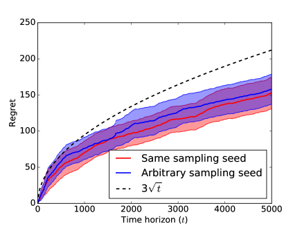
Figure 2: AL-MARL algorithm with the SARL learner of Faradonbeh et al., (2017)

We consider an instance of the MARL2 problem (See Appendix K for the details). The theoretical result of Theorem 2 holds when Assumption 2 is true. Since we use the TS-based learner of Faradonbeh et al., (2017), this assumption can be satisfied by setting the same sampling seed between the agents. Here, we consider both cases of same sampling seed and arbitrary sampling seed for the experiments. We ran 100 simulations and show the mean of regret with the 95% confidence interval for each scenario.

As it can be seen from Figure 2, for both of theses cases, our proposed algorithm with the TS-based learner $\mathcal{L}$ of Faradonbeh et al., (2017) achieves a $\tilde{O}(\sqrt{T})$ regret for our MARL2 problem, which matches the theoretical results of Corollary 1.

7 Conclusion

In this paper, we tackled the challenging problem of regret analysis in Multi-Agent Reinforcement Learning (MARL). We attempted to solve this challenge in the context of online decentralized learning in multi-agent linear-quadratic (LQ) dynamical systems. First, we showed that if a system is unknown, then all the agents should receive information about the state of this system; otherwise, there is no learning policy that can guarantee sub-linear regret for all instances of the decentralized MARL problem. Further, when a system is unknown but there is one-directional communication from the agent controlling the unknown system to the other agents, we proposed a MARL algorithm with regret bounded by $\tilde{O}(\sqrt{T})$.

The MARL algorithm is based on the construction of an auxiliary single-agent LQ problem. The auxiliary single-agent problem serves as an implicit coordination mechanism among the learning agents. The state of the auxiliary SARL can be interpreted as an estimate of the state of the overall system that each agent computes based on the common information among them. While there is a strong connection between the MARL and auxiliary SARL problems, the MARL problem is not reduced to a SARL problem. In particular, Lemma 5 shows that the costs of the two problems actually differ by a term that depends on the random process $e_{t}$, which is dynamically controlled by the MARL algorithm. Therefore, the auxiliary SARL problem is not equivalent to the MARL problem. Nevertheless, the proposed MARL algorithm can bound the additional regret due to the process $e_{t}$ and achieve the same regret order as a SARL algorithm.

The use of the common state estimate plays a key role in the MARL algorithm. The current theoretical analysis uses this common state estimate along with some properties of LQ structure (e.g. certainty equivalence which connects estimates to optimal control (Kumar and Varaiya,, 2015)) to quantify the regret bound. However, certainty equivalence is often used in general systems with continuous state and action spaces as a heuristic with some good empirical performance. This suggests that our algorithm combined with linear approximation of dynamics could potentially be applied to non-LQ systems as a heuristic. That is, each agent constructs an auxiliary SARL with the common estimate as the state, solves this SARL problem heuristically using approximate linear dynamics and/or certainty equivalence, and then modifies the SARL outputs according to the agent’s private information.

Regret Bounds for Decentralized Learning in Cooperative Multi-Agent Dynamical Systems

(Supplementary File)

Outline. The supplementary material of this paper is organized as follows.

• Appendix A presents the notation which is used throughout this Supplementary File.

• Appendix B presents a set of preliminary results, which are useful in proving the main results of this paper.

• Appendix C provides the proof of Theorem 1.

• Appendix D provides the proof of Theorem 2.

• Appendix E provides the proof of Lemma 10. Note that this lemma has been stated in Appendix D and is required for the proof of Theorem 2.

• Appendix F provides the proof of Lemma 11. Note that this lemma has been stated in Appendix D and is required for the proof of Theorem 2.

• Appendix G provides the proof of Lemma 12. Note that this lemma, which has been stated in Appendix D, is the rephrased version of Lemma 4 in the main submission.

• Appendix H provides the proof of Lemma 13. Note that this lemma, which has been stated in Appendix D, is the rephrased version of Lemma 5 in the main submission.

• Appendix I describes the SARL learner $\mathcal{L}$ of some of existing algorithms for the SARL problems in details.

• Appendix J provides two lemmas. The first lemma (Lemma 15) is the complete version of Lemma 1 which describes optimal strategies for the optimal multi-agent LQ problem of Section 2.1. The second lemma (Lemma 16) describes optimal strategies for the optimal single-agent LQ problem of Section 3.

• Appendix K provides the details of the experiments in the main submission (Section 6).

• Appendix L provides the proof of Theorem 3 which extends Theorem 2 to the case with more than 2 agents.

• Appendix M provides the analysis and the results for unknown $\theta_{*}^{1}$ and $\theta_{*}^{2}$, two-way information sharing ($\gamma^{1}=\gamma^{2}=1$).

Appendix A Notation

In general, subscripts are used as time indices while superscripts are used to index agents. The collection of matrices $A^{1},\ldots,A^{n}$ (resp. vectors $x^{1},\ldots,x^{n}$) is denoted as $A^{1:n}$ (resp. $x^{1:n}$). Given column vectors $x^{1},\ldots,x^{n}$, the notation $\operatorname{\mathbf{vec}}(x^{1:n})$ is used to denote the column vector formed by stacking vectors $x^{1},\ldots,x^{n}$ on top of each other. For two symmetric matrices $A$ and $B$, $A\succeq B$ (resp. $A\succ B$) means that $(A-B)$ is positive semi-definite (PSD) (resp. positive definite (PD)). The trace of matrix $A$ is denoted by $\operatorname{\mathbf{tr}}(A)$.

We use $\left\lVert\cdot\right\rVert_{\bullet}$ to denote the operator norm of matrices. We use $\left\lVert\cdot\right\rVert_{2}$ to denote the spectral norm, that is, $\left\lVert M\right\rVert_{2}$ is the maximum singular value of a matrix $M$. We use $\left\lVert\cdot\right\rVert_{1}$ and $\left\lVert\cdot\right\rVert_{\infty}$ to denote maximum column sum matrix norm and maximum row sum matrix norm, respectively. More specifically, if $M\in\mathbb{R}^{m\times n}$, then $\left\lVert M\right\rVert_{1}=\max_{1\leq j\leq n}\sum_{i=1}^{m}|m_{ij}|$ and $\left\lVert M\right\rVert_{\infty}=\max_{1\leq i\leq m}\sum_{j=1}^{n}|m_{ij}|$ where $m_{ij}$ is the entry at the $i$-th row and $j$-th column of $M$. We further use $\left\lVert\cdot\right\rVert_{\rm F}$ to denote the Frobenius norm, that is, $\left\lVert M\right\rVert_{\rm F}=\sqrt{\sum_{i=1}^{m}\sum_{j=1}^{n}|m_{ij}|^{2}}=\sqrt{\operatorname{\mathbf{tr}}(M^{\intercal}M)}$. The notation $\rho(M)$ refers to the spectral radius of a matrix $M$, i.e., $\rho(M)$ is the largest absolute value of its eigenvalues.

Consider matrices $P,Q,R,A,B$ of appropriate dimensions with $P,Q$ being PSD matrices and $R$ being a PD matrix. We define $\mathcal{R}(P,Q,R,A,B)$ and $\mathcal{K}(P,R,A,B)$ as follows:

$$\mathcal{R}(P,Q,R,A,B):= Q+A^{\intercal}PA-A^{\intercal}PB(R+B^{\intercal}PB)^{-1}B^{\intercal}PA.$$

$$\mathcal{K}(P,R,A,B):= -(R+B^{\intercal}PB)^{-1}B^{\intercal}PA.$$

Note that $P=\mathcal{R}(P,Q,R,A,B)$ is the discrete time algebraic Riccati equation.

We use $[P^{\cdot,\cdot}]_{1:4}$ and $\textbf{diag}(P^{1},\ldots,P^{4})$ to denote the following block matrices,

$$[P^{\cdot,\cdot}]_{1:4}:=\begin{bmatrix}P^{11}&\ldots&\ldots&P^{14}\\ \vdots&\ddots&&\vdots\\ \vdots&&\ddots&\vdots\\ P^{41}&\ldots&\ldots&P^{44}\end{bmatrix},\quad\textbf{diag}(P^{1},\ldots,P^{4})=\begin{bmatrix}P^{1}&\mathbf{0}&\ldots&\mathbf{0}\\ \mathbf{0}&\ddots&\ddots&\vdots\\ \vdots&\ddots&\ddots&\mathbf{0}\\ \mathbf{0}&\ldots&\mathbf{0}&P^{4}\end{bmatrix}$$

Further, we use $[P]_{i,i}$ to denote the block matrix located at the $i$-th row partition and $i$-th column partition of $P$. For example, $[\textbf{diag}(P^{1},\ldots,P^{4})]_{2,2}=P^{2}$ and $[[P^{\cdot,\cdot}]_{1:4}]_{1,1}=P^{11}$.

Appendix B Preliminaries

First, we state a variant of the Hanson-Wright inequality (Hanson and Wright,, 1971) which can be found in Hsu et al., (2012).

Theorem 4 (Hsu et al., (2012)).

Let $X\sim\mathcal{N}(0,\mathbf{I})$ be a Gaussian random vector and let $A\in\mathbb{R}^{m\times n}$ and $\Delta:=A^{\intercal}A$. For all $z>0$,

$$\operatorname{\mathbb{P}}\big{(}\left\lVert AX\right\rVert_{2}^{2}-\operatorname{\mathbb{E}}[\left\lVert AX\right\rVert_{2}^{2}]>2\left\lVert\Delta\right\rVert_{\rm F}\sqrt{z}+2\left\lVert\Delta\right\rVert_{2}z\big{)}\leq\exp(-z).$$ (14)

Lemma 6.

Let $A\in\mathbb{R}^{l\times m},B\in\mathbb{R}^{m\times n}$. Then, $\left\lVert AB\right\rVert_{\rm F}\leq\left\lVert A\right\rVert_{2}\left\lVert B\right\rVert_{\rm F}$.

Proof.

Let $B=[b_{1},\ldots,b_{n}]$ be the column partitioning of $B$. Then,

$$\left\lVert AB\right\rVert_{\rm F}^{2}=\sum_{i=1}^{n}\left\lVert Ab_{i}\right\rVert_{2}^{2}\leq\left\lVert A\right\rVert_{2}^{2}\sum_{i=1}^{n}\left\lVert b_{i}\right\rVert_{2}^{2}=\left\lVert A\right\rVert_{2}^{2}\left\lVert B\right\rVert_{\rm F}^{2},$$ (15)

where the first equality follows from the definition of Frobenius norm, the first inequality is correct because the operator norm is a sub-multiplicative matrix norm, and the last equality follows from the definition of Frobenius norm. ∎

Using Theorem 4 and Lemma 6, we can state the following result.

Lemma 7.

Let $X\sim\mathcal{N}(0,\mathbf{I})$ be a Gaussian random vector and let $A\in\mathbb{R}^{m\times n}$. Then for any $\delta\in(0,1/e)$, we have

$$\left\lVert AX\right\rVert_{2}^{2}-\operatorname{\mathbf{tr}}(A^{\intercal}A)\leq 4\left\lVert A\right\rVert_{2}\left\lVert A\right\rVert_{\rm F}\log(\frac{1}{\delta}),$$ (16)

with probability at least $1-\delta$.

Proof.

Since $X\sim\mathcal{N}(0,\mathbf{I})$, from Theorem 4, for any $z>1$, we have with probability at least $1-\exp(-z)$,

$$\left\lVert AX\right\rVert_{2}^{2}-\operatorname{\mathbf{tr}}(A^{\intercal}A) \leq 2\left\lVert\Delta\right\rVert_{\rm F}\sqrt{z}+2\left\lVert\Delta\right\rVert_{2}z\leq 2\left\lVert A\right\rVert_{2}\left\lVert A\right\rVert_{\rm F}\sqrt{z}+2\left\lVert A\right\rVert_{2}\left\lVert A\right\rVert_{2}z$$

$$\leq 2\left\lVert A\right\rVert_{2}\left\lVert A\right\rVert_{\rm F}z+2\left\lVert A\right\rVert_{2}\left\lVert A\right\rVert_{\rm F}z\leq 4\left\lVert A\right\rVert_{2}\left\lVert A\right\rVert_{\rm F}z,$$ (17)

where the second inequality is correct because of Lemma 6 and the third inequality is correct because $z>1$ and $\left\lVert A\right\rVert_{2}\leq\left\lVert A\right\rVert_{\rm F}$. Now by choosing $z=\log(\frac{1}{\delta})$ where $\delta\in(0,1/e)$ the correctness of Lemma 7 is obtained. ∎

Lemma 8 (Lemma 5.6.10 (Horn and Johnson,, 1990)).

Let $A\in\mathbb{R}^{n\times n}$ and $\epsilon>0$ be given. There is a matrix norm $\left\lVert\cdot\right\rVert_{\bullet}$ such that $\rho(A)\leq\left\lVert A\right\rVert_{\bullet}\leq\rho(A)+\epsilon$.

The above lemma implies the following results.

Corollary 2.

Let $A\in\mathbb{R}^{n\times n}$ and $\rho(A)<1$. Then, there exists some matrix norm $\left\lVert\cdot\right\rVert_{\bullet}$ such that $\left\lVert A\right\rVert_{\bullet}<1$.

Lemma 9.

Let $A$ be a $d\times d$ block matrix where $A_{i,j}\in\mathbb{R}^{n\times n}$ denotes the block matrix at the $i$-th row partition and $j$-th column partition. Then,

$$\left\lVert A\right\rVert_{\infty} =\max_{j=1,\ldots,d}\left\lVert\sum_{i=1}^{d}\tilde{A}_{i,j}\right\rVert_{\infty},\quad\left\lVert A\right\rVert_{1}=\max_{i=1,\ldots,d}\left\lVert\sum_{j=1}^{d}\tilde{A}_{i,j}\right\rVert_{1},$$ (18)

where matrix $\tilde{A}_{i,j}$ is the entry-wise absolute value of matrix $A_{i,j}$.

Proof.

We prove the equality for $\left\lVert A\right\rVert_{\infty}$. The proof for $\left\lVert A\right\rVert_{1}$ can be obtained in a similar way. Note that,

$$\max_{i=1,\ldots,d}\left\lVert\sum_{j=1}^{d}\tilde{A}_{i,j}\right\rVert_{\infty}=\max_{i=1,\ldots,d}\max_{k_{i}=1,\ldots,n}\sum_{j=1}^{d}\sum_{k_{j}=1}^{n}|\tilde{a}_{k_{i}k_{j}}|=\max_{1\leq i\leq nd}\sum_{j=1}^{nd}|a_{ij}|=\left\lVert A\right\rVert_{\infty}$$ (19)

where $\tilde{a}_{ij}$ is the entry at the $i$-th row and $j$-th column of $\tilde{A}$. ∎

Appendix C Proof of Theorem 1

We want to show that there is no algorithm that can achieve a lower-bound better than $\Omega(T)$ on the regret of all instances of the MARL1 problem. Equivalently, we can show that for any algorithm, there is an instance of the MARL1 problem whose regret is at least $\Omega(T)$. To this end, consider an instance of the MARL1 problem where the systems dynamics and the cost function are described as follows,

$$x_{t+1}^{1}=u_{t}^{1},\quad x_{t+1}^{2}=a_{*}^{2}x_{t}^{2},\quad\quad x_{0}^{1}=x_{0}^{2}=1,$$ (20)

$$c(x_{t},u_{t})=(x_{t}^{1}-x_{t}^{2})^{2}+(u_{t}^{1}-0.5u_{t}^{2})^{2}.$$ (21)

We assume that the only unknown parameter is $a_{*}^{2}$. Note that for any $a_{*}^{2}\in(-1,1)$, the above problem satisfies Assumption 1. By using (20), the cost function of (21) can be rewritten as,

$$c(x_{t},u_{t})=(u_{t-1}^{1}-(a_{*}^{2})^{t})^{2}+(u_{t}^{1}-0.5u_{t}^{2})^{2}.$$ (22)

If $a_{*}^{2}$ is known to the both controllers, one can easily show that the optimal infinite horizon average cost is 0 and it is achieved by setting $u_{t}^{1}=(a_{*}^{2})^{t+1}$ and $u_{t}^{2}=2(a_{*}^{2})^{t+1}$.

If $a_{*}^{2}$ in unknown, the regret of any policy $\pi$ can be written as,

$$R(T,\pi) =\sum_{t=0}^{T-1}c(x_{t},u_{t})=(u_{0}^{1}-0.5u_{0}^{2})^{2}+\sum_{t=1}^{T-1}\left[(u_{t-1}^{1}-(a_{*}^{2})^{t})^{2}+(u_{t}^{1}-0.5u_{t}^{2})^{2}\right]$$

$$\geq\sum_{t=1}^{T-1}(u_{t-1}^{1}-(a_{*}^{2})^{t})^{2},$$ (23)

where the first equality is correct due to the fact that the optimal infinite horizon average cost is 0, the second equality is correct because of (22) and the fact that $x_{0}^{1}=x_{0}^{2}=1$, and the first inequality is correct because $(u_{t}^{1}-0.5u_{t}^{2})^{2}\geq 0$. Now, we show that for any policy $\pi$, there is a value for $a_{*}^{2}$ such that $R(T,\pi)\geq\Omega(T)$. This is equivalent to show that $\sup_{a_{*}^{2}\in(-1,1)}R(T,\pi)\geq\Omega(T)$. This can be shown as follows,

$$\sup_{a_{*}^{2}\in(-1,1)}R(T,\pi)\geq\sup_{a_{*}^{2}\in(-1,1)}\sum_{t=1}^{T-1}(u_{t-1}^{1}-(a_{*}^{2})^{t})^{2}\geq\frac{1}{2}\sum_{t=1}^{T-1}(u_{t-1}^{1}-0)^{2}+\frac{1}{2}\sum_{t=1}^{T-1}(u_{t-1}^{1}-\alpha^{t})^{2}$$

$$=\sum_{t=1}^{T-1}\left[(u_{t-1}^{1}-\frac{\alpha^{t}}{2})^{2}+\frac{\alpha^{2t}}{2}-\frac{\alpha^{2t}}{4}\right]\geq\sum_{t=1}^{T-1}\frac{\alpha^{2t}}{4}=\frac{\alpha^{2}(1-\alpha^{2T})}{4(1-\alpha^{2})},\quad\forall\alpha\in(-1,1),$$ (24)

where the first inequality is correct because supremum over a set is greater than or equal to expectation with respect to any distribution over that set. Further, the second equality is correct because $(u_{t-1}^{1}-\frac{1}{2})^{2}\geq 0$. Since (25) is true for any $\alpha\in(-1,1)$, it holds also for limit when $\alpha\rightarrow 1^{-}$. By taking the limit, we can obtain

$$\sup_{a_{*}^{2}\in(-1,1)}R(T,\pi)\geq\lim_{\alpha\to 1^{-}}\frac{\alpha^{2}(1-\alpha^{2T})}{4(1-\alpha^{2})}=\frac{T}{4}=\Omega(T).$$ (25)

This completes the proof.

Appendix D Proof of Theorem 2

We first state some preliminary results in the following lemmas which will be used in the proof of Theorem 2.

Lemma 10.

Let $s_{t}$ be a random process that evolves as follows,

$$s_{t+1}=Cs_{t}+v_{t},\quad s_{0}=0,$$ (26)

where $v_{t}$, $t\geq 0$, are independent Gaussian random vectors with zero-mean and covariance matrix $\operatorname{\mathbf{cov}}(v_{t})=\mathbf{I}$. Further, let $C=A_{*}^{2}+B_{*}^{2}\tilde{K}^{2}(\theta_{*}^{2})$ and define $\Sigma_{t}=\operatorname{\mathbf{cov}}(s_{t})$, then the sequence of matrices $\Sigma_{t}$, $t\geq 0$, is increasing and it converges to a PSD matrix $\Sigma$ as $t\to\infty$. Further, $C$ is a stable matrix, that is, $\rho(C)<1$.

Proof.

See Appendix E for a proof. ∎

Lemma 11.

Let $s_{t}$ be a random process defined as in Lemma 10. Let $D$ be a positive semi-definite (PSD) matrix. Then for any $\delta\in(0,1/e)$, with probability at least $1-\delta$,

$$\sum_{t=1}^{T}[s_{t}^{\intercal}Ds_{t}-\operatorname{\mathbf{tr}}(D\Sigma)]\leq\log(\frac{1}{\delta})\tilde{K}\sqrt{T}.$$ (27)

Proof.

See Appendix F for a proof. ∎

We now proceed in two steps:

• Step 1: Showing the connection between the auxiliary SARL problem and the MARL2 problem

• Step 2: Using the SARL problem to bound the regret of the MARL2 problem

Step 1: Showing the connection between the auxiliary SARL problem and the MARL2 problem

First, we present the following lemma that connects the optimal infinite horizon average cost $J^{\diamond}(\theta_{*}^{1,2})$ of the auxiliary SARL problem when $\theta_{*}^{1,2}$ are known (that is, the auxiliary single-agent LQ problem of Section 3) and the optimal infinite horizon average cost $J(\theta_{*}^{1,2})$ of the MARL2 problem when $\theta_{*}^{1,2}$ are known (that is, the multi-agent LQ problem of Section 2.1).

Lemma 12 (rephrased version of Lemma 4).

Let $J^{\diamond}(\theta_{*}^{1,2})$ be the optimal infinite horizon average cost of the auxiliary SARL problem, $J(\theta_{*}^{1,2})$ be the optimal infinite horizon average cost of the MARL2 problem, and $\Sigma$ be as defined in Lemma 10. Then,

$$J(\theta_{*}^{1,2})=J^{\diamond}(\theta_{*}^{1,2})+\operatorname{\mathbf{tr}}(D\Sigma),$$ (28)

where we have defined $D:=Q^{22}+(\tilde{K}^{2}(\theta_{*}^{2}))^{\intercal}R^{22}\tilde{K}^{2}(\theta_{*}^{2})$.

Proof.

See Appendix G for a proof. ∎

Next, we provide the following lemma that shows the connection between the cost $c(x_{t},u_{t})$ in the MARL2 problem under the policy of the AL-MARL algorithm and the cost $c(x_{t}^{\diamond},u_{t}^{\diamond})$ in the auxiliary SARL problem under the policy of the AL-SARL algorithm.

Lemma 13 (rephrased version of Lemma 5).

At each time $t$, the following equality holds between the cost under the policies of the AL-SARL and the AL-MARL algorithms,

$$c(x_{t},u_{t})|_{\texttt{AL-MARL}} =c(x_{t}^{\diamond},u_{t}^{\diamond})|_{\texttt{AL-SARL}}+e_{t}^{\intercal}De_{t},$$ (29)

where $e_{t}=x_{t}^{2}-\check{x}_{t}^{2}$ and $D=Q^{22}+(\tilde{K}^{2}(\theta_{*}^{2}))^{\intercal}R^{22}\tilde{K}^{2}(\theta_{*}^{2})$.

Proof.

See Appendix H for a proof. ∎

Step 2: Using the SARL problem to bound the regret of the MARL2 problem

In this step, we use the connection between the auxiliary SARL problem and our MARL2 problem, which was established in Step 1, to prove Theorem 2. Note that from the definition of the regret in the MARL problem given by (8), we have,

$$R(T,\texttt{AL-MARL})=\sum_{t=0}^{T-1}\left[c(x_{t},u_{t})|_{\texttt{AL-MARL}}-J(\theta_{*}^{1,2})\right]$$

$$=\sum_{t=0}^{T-1}\left[c(x_{t}^{\diamond},u_{t}^{\diamond})|_{\texttt{AL-SARL}}-J^{\diamond}(\theta_{*}^{1,2})\right]+\sum_{t=0}^{T-1}\left[e_{t}^{\intercal}De_{t}-\operatorname{\mathbf{tr}}(D\Sigma)\right]\leq R^{\diamond}(T,\texttt{AL-SARL})+\log(\frac{1}{\delta})\tilde{K}\sqrt{T}$$ (30)

where the second equality is correct because of Lemma 12 and Lemma 13. Further, if we define $v_{t}:=w_{t}^{2}$, $e_{t}$ has the same dynamics as $s_{t}$ in Lemma 11. Then, the last inequality is correct because of Lemma 11 and the definition of the regret in the SARL problem given by in (11). This proves the statement of Theorem 2.

Appendix E Proof of Lemma 10

First, note that $\Sigma_{t}$ can be sequentially calculated as $\Sigma_{t+1}=\mathbf{I}+C\Sigma_{t}C^{\intercal}$ with $\Sigma_{0}=\mathbf{0}$. Now, we use induction to show that the sequence of matrices $\Sigma_{t}$, $t\geq 0$, is increasing. First, we can write $\Sigma_{t+1}-\Sigma_{t}=C(\Sigma_{t}-\Sigma_{t-1})C^{\intercal}$. Then, since $\Sigma_{0}=\mathbf{0}$ and $\Sigma_{1}=\mathbf{I}\succeq\mathbf{0}$, we have $\Sigma_{1}-\Sigma_{0}\succeq\mathbf{0}$. Now, assume that $\Sigma_{t}-\Sigma_{t-1}\succeq\mathbf{0}$. Then, it is easy to see that $\Sigma_{t+1}-\Sigma_{t}=C(\Sigma_{t}-\Sigma_{t-1})C^{\intercal}\succeq\mathbf{0}$.

To show that the sequence of matrices $\Sigma_{t}$, $t\geq 0$, converges to $\Sigma$ as $t\to\infty$, first we show that $C$ is stable, that is, $\rho(C)<1$. Note that $C=A_{*}^{2}+B_{*}^{2}\tilde{K}^{2}(\theta_{*}^{2})$ where from (66), we have

$$\tilde{K}^{2}(\theta_{*}^{2}) =\mathcal{K}(\tilde{P}^{2}(\theta_{*}^{2}),R^{22},A_{*}^{2},B_{*}^{2}),$$

$$\tilde{P}^{2}(\theta_{*}^{2}) =\mathcal{R}(\tilde{P}^{2}(\theta_{*}^{2}),Q^{22},R^{22},A_{*}^{2},B_{*}^{2}).$$ (31)

Then, from Assumption 1, $(A_{*},B_{*})$ is stabilizable and since both of $A_{*}$ and $B_{*}$ are block diagonal matrices, $(A_{*}^{2},B_{*}^{2})$ is stabilizable. Hence, we know from Costa et al., (2006, Theorem 2.21) that $\rho(C)<1$. Since $C$ is stable, the converges of the sequence of matrices $\Sigma_{t}$, $t\geq 0$, can be concluded from Kumar and Varaiya, (2015, Chapter 3.3).

Appendix F Proof of Lemma 11

In this proof, we use superscripts to denote exponents.

Step 1:

Lemma 14.

Let $s_{t}$ be as defined in (26). Then,

$$\sum_{t=1}^{T}[s_{t}^{\intercal}Ds_{t}-\operatorname{\mathbf{tr}}(D\Sigma_{t})]=\bar{v}^{\intercal}L^{\intercal}L\bar{v}-\operatorname{\mathbf{tr}}(L^{\intercal}L),$$ (32)

where $L=\bar{D}^{1/2}\bar{C}$ and

$$\bar{v}=\begin{bmatrix}v_{0}\\ v_{1}\\ \vdots\\ v_{T-1}\end{bmatrix},\quad\bar{C}=\begin{bmatrix}\mathbf{I}&\mathbf{0}&\ldots&\ldots&\mathbf{0}\\ C&\mathbf{I}&\mathbf{0}&&\vdots\\ C^{2}&C&\mathbf{I}&\ddots&\vdots\\ \vdots&\vdots&\ddots&\ddots&\mathbf{0}\\ C^{T-1}&C^{T-2}&\ldots&C&\mathbf{I}\end{bmatrix},\quad\bar{D}=\begin{bmatrix}D&\mathbf{0}&\ldots&\ldots&\mathbf{0}\\ \mathbf{0}&D&\mathbf{0}&&\vdots\\ \mathbf{0}&\mathbf{0}&D&\ddots&\vdots\\ \vdots&\vdots&\ddots&\ddots&\mathbf{0}\\ \mathbf{0}&\mathbf{0}&\ldots&\mathbf{0}&D\end{bmatrix}.$$ (33)

Proof.

First note that from (26), $s_{t}$ can be written as,

$$s_{t}=\sum_{i=0}^{t-1}C^{t-1-i}v_{i}+\sum_{i=t}^{T-1}\mathbf{0}\times v_{i}=\begin{bmatrix}C^{t-1}&C^{t-2}&\ldots&C&\mathbf{I}&\mathbf{0}&\ldots&\mathbf{0}\end{bmatrix}\bar{v}.$$ (34)

Furthermore, since $D$ and consequently, $\bar{D}$ are PSD matrices, there exists $\bar{D}^{1/2}$ such that $\bar{D}=(\bar{D}^{1/2})^{\intercal}\bar{D}^{1/2}$ (similarly, $D=(D^{1/2})^{\intercal}D^{1/2}$). Then, the correctness of (32) is obtained through straightforward algebraic manipulations. ∎

Step 2:

Since from Lemma 14, $\bar{v}$ in is Gaussian, we can apply Lemma 7 to bound $\bar{v}^{\intercal}L^{\intercal}L\bar{v}-\operatorname{\mathbf{tr}}(L^{\intercal}L)$ as follows. For any $\delta\in(0,1/e)$, we have with probability at least $1-\delta$,

$$\bar{v}^{\intercal}L^{\intercal}L\bar{v}-\operatorname{\mathbf{tr}}(L^{\intercal}L)\leq 4\left\lVert L\right\rVert_{2}\left\lVert L\right\rVert_{\rm F}\log(\frac{1}{\delta}).$$ (35)

Step 3:

In this step, we find an upper-bound for $\left\lVert L\right\rVert_{\rm F}$. To this end, first note that by definition, we have $\left\lVert L\right\rVert_{\rm F}=\sqrt{\operatorname{\mathbf{tr}}(L^{\intercal}L)}$. From (33), we can write $L$ as follows,

$$L=\begin{bmatrix}D^{1/2}&\mathbf{0}&\ldots&\ldots&\mathbf{0}\\ D^{1/2}C&D^{1/2}&\mathbf{0}&&\vdots\\ D^{1/2}C^{2}&D^{1/2}C&D^{1/2}&\ddots&\vdots\\ \vdots&\vdots&\ddots&\ddots&\mathbf{0}\\ D^{1/2}C^{T-1}&D^{1/2}C^{T-2}&\ldots&D^{1/2}C&D^{1/2}\end{bmatrix}.$$ (36)

Then, using (36), we have

$$L^{\intercal}L=\begin{bmatrix}\sum_{i=0}^{T-1}(C^{i})^{\intercal}DC^{i}&\mathbf{\times}&\ldots&\ldots&\mathbf{\times}\\ \mathbf{\times}&\sum_{i=0}^{T-2}(C^{i})^{\intercal}DC^{i}&\mathbf{\times}&&\vdots\\ \mathbf{\times}&\mathbf{\times}&\sum_{i=0}^{T-3}(C^{i})^{\intercal}DC^{i}&\ddots&\vdots\\ \vdots&\vdots&\ddots&\ddots&\mathbf{\times}\\ \mathbf{\times}&\mathbf{\times}&\ldots&\mathbf{\times}&D\end{bmatrix}.$$ (37)

Now, from (37) and the fact that trace is a linear operator, we can write,

$$\operatorname{\mathbf{tr}}(L^{\intercal}L)=\sum_{j=0}^{T-1}\sum_{i=0}^{j}\operatorname{\mathbf{tr}}\big{(}(C^{i})^{\intercal}DC^{i}\big{)}.$$ (38)

In the following, we find an upper-bound for $\operatorname{\mathbf{tr}}\big{(}(C^{i})^{\intercal}DC^{i}\big{)}$. Since $D$ is a PSD matrix, we can write it as $D=\sum_{l=1}^{r}d_{l}d_{l}^{T}$ where $r$ is rank of matrix $D$. By using this, we can have,

$$\operatorname{\mathbf{tr}}\big{(}(C^{i})^{\intercal}DC^{i}\big{)} =\operatorname{\mathbf{tr}}\big{(}(C^{i})^{\intercal}\sum_{l=1}^{r}d_{l}d_{l}^{T}C^{i}\big{)}\stackrel{{\scriptstyle(*1)}}{{=}}\sum_{l=1}^{r}\operatorname{\mathbf{tr}}\big{(}(C^{i})^{\intercal}d_{l}d_{l}^{T}C^{i}\big{)}\stackrel{{\scriptstyle(*2)}}{{=}}\sum_{l=1}^{r}\left\lVert(C^{i})^{\intercal}d_{l}\right\rVert_{2}^{2}$$

$$\leq\sum_{l=1}^{r}\left\lVert(C^{i})^{\intercal}\right\rVert_{2}^{2}\left\lVert d_{l}\right\rVert_{2}^{2}\leq\left\lVert C\right\rVert_{2}^{2i}\sum_{l=1}^{r}\left\lVert d_{l}\right\rVert_{2}^{2}=\left\lVert C\right\rVert_{2}^{2i}\operatorname{\mathbf{tr}}(D)\stackrel{{\scriptstyle(*3)}}{{\leq}}\beta\left\lVert C\right\rVert_{\bullet}^{2i}\operatorname{\mathbf{tr}}(D)$$

$$\stackrel{{\scriptstyle(*4)}}{{=}}\beta\alpha^{2i}\operatorname{\mathbf{tr}}(D),$$ (39)

where $(*1)$ is correct because $\operatorname{\mathbf{tr}}(\cdot)$ is a linear operator and $(*2)$ is correct because if $v$ is a column vector, then $\operatorname{\mathbf{tr}}(vv^{\intercal})=\left\lVert v\right\rVert_{2}^{2}$. Further, $(*3)$ is correct because any two norms on a finite dimensional space are equivalent. In other words, for any norm $\left\lVert\cdot\right\rVert_{\bullet}$, there is a number $\beta$ such that $\left\lVert C\right\rVert_{2}\leq\beta\left\lVert C\right\rVert_{\bullet}$. Note that $\beta$ is independent of $T$. Now, let the second norm (that is, $\left\lVert\cdot\right\rVert_{\bullet}$) be the norm for which $\left\lVert C\right\rVert_{\bullet}<1$ (note that since $\rho(C)<1$, the existence of this norm follows form Corollary 2). Then, the correctness of $(*4)$ is resulted by defining $\alpha:=\left\lVert C\right\rVert_{\bullet}<1$.

From (39), we can write,

$$\sum_{i=0}^{j}\operatorname{\mathbf{tr}}\big{(}(C^{i})^{\intercal}DC^{i}\big{)}\leq\beta\operatorname{\mathbf{tr}}(D)\sum_{i=0}^{j}\alpha^{2i}\leq\beta\operatorname{\mathbf{tr}}(D)\sum_{i=0}^{\infty}\alpha^{2i}=\beta\frac{\operatorname{\mathbf{tr}}(D)}{1-\alpha^{2}}.$$ (40)

Finally, using (38) and (40), we have $\operatorname{\mathbf{tr}}(L^{\intercal}L)\leq T\beta\frac{\operatorname{\mathbf{tr}}(D)}{1-\alpha^{2}}$ which means that

$$\left\lVert L\right\rVert_{\rm F}=\sqrt{\operatorname{\mathbf{tr}}(L^{\intercal}L)}\leq\sqrt{T\beta\frac{\operatorname{\mathbf{tr}}(D)}{1-\alpha^{2}}}.$$ (41)

Step 4:

In this step, we find an upper-bound for $\left\lVert L\right\rVert_{2}$. We use $\left\lVert L\right\rVert_{2}\leq\sqrt{\left\lVert L\right\rVert_{1}\left\lVert L\right\rVert_{\infty}}$ to bound $\left\lVert L\right\rVert_{2}$ (Golub and Van Loan,, 1996). To this end, we calculate $\left\lVert L\right\rVert_{1}$ and $\left\lVert L\right\rVert_{\infty}$.

Scalar case:

Because of the special structure of matrix $L$ in (36), these two matrix norms are the same and they are equal to sum of the entries of the first column,

$$\left\lVert L\right\rVert_{1}=\left\lVert L\right\rVert_{\infty}=\sum_{i=0}^{T-1}|D^{1/2}C^{i}|\leq D^{1/2}\sum_{i=0}^{T-1}|C^{i}|\leq D^{1/2}\sum_{i=0}^{T-1}|C|^{i}\leq D^{1/2}\sum_{i=0}^{\infty}\alpha^{i}=\frac{D^{1/2}}{1-\alpha}.$$ (42)

Using (42), we can bound $\left\lVert L\right\rVert_{2}$ as follows,

$$\left\lVert L\right\rVert_{2}\leq\frac{D^{1/2}}{1-\alpha}.$$ (43)

Matrix case:

Since $L$ is a $T\times T$ block matrix, we can write

$$\left\lVert L\right\rVert_{\infty} =\max_{i=1,\ldots,T}\left\lVert\sum_{j=1}^{T}\tilde{L}_{i,j}\right\rVert_{\infty}\stackrel{{\scriptstyle(*1)}}{{=}}\left\lVert\sum_{j=1}^{T}\tilde{L}_{i,1}\right\rVert_{\infty}\stackrel{{\scriptstyle(*2)}}{{\leq}}\sum_{j=1}^{T1}\left\lVert\tilde{L}_{i,1}\right\rVert_{\infty}\stackrel{{\scriptstyle(*3)}}{{\leq}}\sqrt{K}\sum_{j=1}^{T}\left\lVert\tilde{L}_{i,1}\right\rVert_{2}$$

$$\stackrel{{\scriptstyle(*4)}}{{\leq}}\sqrt{K}\sum_{j=1}^{T}\left\lVert\tilde{L}_{i,1}\right\rVert_{\rm F}\stackrel{{\scriptstyle(*5)}}{{=}}\sqrt{K}\sum_{j=1}^{T}\left\lVert L_{i,1}\right\rVert_{\rm F}\stackrel{{\scriptstyle(*6)}}{{=}}\sqrt{K}\sum_{i=0}^{T-1}\left\lVert D^{1/2}C^{i}\right\rVert_{\rm F}$$

$$\stackrel{{\scriptstyle(*7)}}{{=}}\sqrt{K}\sum_{i=0}^{T-1}\sqrt{\operatorname{\mathbf{tr}}\big{(}(C^{i})^{\intercal}DC^{i}\big{)}}$$

$$\stackrel{{\scriptstyle(*8)}}{{\leq}}\sqrt{K}\sum_{i=0}^{T-1}\alpha^{i}\sqrt{\beta\operatorname{\mathbf{tr}}(D)}\leq\sqrt{K\beta\operatorname{\mathbf{tr}}(D)}\sum_{i=0}^{\infty}\alpha^{i}=\frac{\sqrt{K\beta\operatorname{\mathbf{tr}}(D)}}{1-\alpha},$$ (44)

where matrix $\tilde{L}_{i,j}$ is the entry-wise absolute value of matrix $L_{i,j}$. Note that $(*1)$ is correct because the maximum is achieved by setting $j=1$ (i.e, the first column partition) and $(*2)$ is correct because of the sub-additive property of the norm. For $(*3)$, first note that for any matrix $M\in\mathbb{R}^{n\times n}$, we have $\left\lVert M\right\rVert_{\infty}\leq\sqrt{n}\left\lVert M\right\rVert_{2}$. If we define $K$ to be maximum of size of matrices $\tilde{L}_{i,j}$, then the correctness of $(*3)$ is resulted. Further, $(*4)$ is correct because for any matrix $M$, $\left\lVert M\right\rVert_{2}\leq\left\lVert M\right\rVert_{\rm F}$, $(*5)$ is correct because the Frobenius norm of a matrix and its entry-wise absolute value is the same, $(*6)$ is correct because $L_{i,1}=D^{1/2}C^{i}$, and $(*7)$ follows from the definition of the Frobenius norm. Finally, $(*8)$ is correct because of (39). Similarly, we can show that $\left\lVert L\right\rVert_{1}\leq\frac{\sqrt{K\beta\operatorname{\mathbf{tr}}(D)}}{1-\alpha}$. Hence, we can bound $\left\lVert L\right\rVert_{2}$ as follows,

$$\left\lVert L\right\rVert_{2}\leq\frac{\sqrt{K\beta\operatorname{\mathbf{tr}}(D)}}{1-\alpha}.$$ (45)

Step 5:

By combining the results of Steps 1 to 4, we have with probability at least $1-\delta$,

$$\sum_{t=1}^{T}[s_{t}^{\intercal}Ds_{t}-\operatorname{\mathbf{tr}}(D\Sigma)] =\sum_{t=1}^{T}[s_{t}^{\intercal}Ds_{t}-\operatorname{\mathbf{tr}}(D\Sigma_{t})]+\sum_{t=1}^{T}[\operatorname{\mathbf{tr}}(D\Sigma_{t})-\operatorname{\mathbf{tr}}(D\Sigma)]$$

$$\leq\sum_{t=1}^{T}[s_{t}^{\intercal}Ds_{t}-\operatorname{\mathbf{tr}}(D\Sigma_{t})]\leq 4\frac{\sqrt{K\beta\operatorname{\mathbf{tr}}(D)}}{1-\alpha}\sqrt{T\beta\frac{\operatorname{\mathbf{tr}}(D)}{1-\alpha^{2}}}\log(\frac{1}{\delta}),$$ (46)

where the first inequality is correct because from Lemma 10, the sequence of matrices $\Sigma_{t}$ is increasing, that is, $\Sigma-\Sigma_{t}\succeq\mathbf{0}$ and $D$ is positive semi-definite, and consequently, $\operatorname{\mathbf{tr}}(D(\Sigma_{t}-\Sigma))\leq 0$. Define $\tilde{K}:=\frac{4\beta\sqrt{K}\operatorname{\mathbf{tr}}(D)}{(1-\alpha)\sqrt{1-\alpha^{2}}}$, then the correctness of Lemma 11 is obtained.

Appendix G Proof of Lemma 12 (Lemma 4)

Let $\pi^{\diamond*}$ be optimal policy for the auxiliary SARL problem when $\theta_{*}^{1,2}$ are known. Then, the optimal infinite horizon average cost under $\theta_{*}^{1,2}$ of this auxiliary SARL problem can be written as,

$$J^{\diamond}(\theta_{*}^{1,2})=\limsup_{T\rightarrow\infty}\frac{1}{T}\sum_{t=0}^{T-1}\operatorname{\mathbb{E}}^{\pi^{\diamond*}}[c(x_{t}^{\diamond},u_{t}^{\diamond})|\theta_{*}^{1,2}].$$ (47)

Under the optimal policy $\pi^{\diamond*}$ (see Lemma 16 in Appendix J), $u_{t}^{\diamond}=K(\theta_{*}^{1,2})x_{t}^{\diamond}$ and hence, the dynamics of $x_{t}^{\diamond}$ in (9) can be written as,

$$x_{t+1}^{\diamond}=\Big{(}A_{*}+B_{*}K(\theta_{*}^{1,2})\Big{)}x_{t}^{\diamond}+\operatorname{\mathbf{vec}}(w_{t}^{1},\mathbf{0}).$$ (48)

Further, let $\pi^{*}$ be optimal policy for the MARL problem when $\theta_{*}^{1,2}$ is known. Then, from (5) we have,

$$J(\theta_{*}^{1,2})=\limsup_{T\rightarrow\infty}\frac{1}{T}\sum_{t=0}^{T-1}\operatorname{\mathbb{E}}^{\pi^{*}}[c(x_{t},u_{t})|\theta_{*}^{1,2}].$$ (49)

From Lemma 1, we know that under the optimal policy $\pi^{*}$,

$$u_{t}=K(\theta_{*}^{1,2})\bar{x}_{t}+\operatorname{\mathbf{vec}}(\mathbf{0},\tilde{K}^{2}(\theta_{*}^{2})e_{t}),$$ (50)

where we have defined $\bar{x}_{t}:=\operatorname{\mathbf{vec}}(x_{t}^{1},\hat{x}_{t}^{2})$, $e_{t}:=x_{t}^{2}-\hat{x}_{t}^{2}$, and we have $K(\theta_{*}^{1,2})=\begin{bmatrix}K^{1}(\theta_{*}^{1,2})\\ K^{2}(\theta_{*}^{1,2})\end{bmatrix}$ from Lemma 15 in the Appendix J. Then, from the dynamics of $x_{t}$ in (2) and update equation for $\hat{x}_{t}^{2}$ in (7), we can write

$$x_{t+1}=\bar{x}_{t+1}+\operatorname{\mathbf{vec}}(\mathbf{0},e_{t+1}),$$ (51)

where

$$\bar{x}_{t+1} =\Big{(}A_{*}+B_{*}K(\theta_{*}^{1,2})\Big{)}\bar{x}_{t}+\operatorname{\mathbf{vec}}(w_{t}^{1},\mathbf{0}),\quad e_{t+1}=Ce_{t}+w_{t}^{2}.$$ (52)

Note that we have defined $C=A_{*}^{2}+B_{*}^{2}\tilde{K}^{2}(\theta_{*}^{2})$. Now by comparing (48) and (52) and the fact that both $x_{1}^{\diamond}$ and $\bar{x}_{1}$ are equal, we can see that for any time $t$,

$$\bar{x}_{t+1}=x_{t+1}^{\diamond}.$$ (53)

Now, we can use the above results to write $\operatorname{\mathbb{E}}^{\pi^{*}}[c(x_{t},u_{t})|\theta_{*}^{1,2}]$ as follows,

$$\operatorname{\mathbb{E}}^{\pi^{*}}[c(x_{t},u_{t})|\theta_{*}^{1,2}]=\operatorname{\mathbb{E}}^{\pi^{*}}[x_{t}^{\intercal}Qx_{t}+(u_{t})^{\intercal}Ru_{t}|\theta_{*}^{1,2}]$$

$$=\operatorname{\mathbb{E}}^{\pi^{*}}[\bar{x}_{t}^{\intercal}Q\bar{x}_{t}+(K(\theta_{*}^{1,2})\bar{x}_{t})^{\intercal}RK(\theta_{*}^{1,2})\bar{x}_{t}|\theta_{*}^{1,2}]+\operatorname{\mathbb{E}}[e_{t}^{\intercal}De_{t}|\theta_{*}^{1,2}]$$

$$=\operatorname{\mathbb{E}}^{\pi^{\diamond*}}[(x_{t}^{\diamond})^{\intercal}Qx_{t}^{\diamond}+(K(\theta_{*}^{1,2})x_{t}^{\diamond})^{\intercal}RK(\theta_{*}^{1,2})x_{t}^{\diamond}|\theta_{*}^{1,2}]+\operatorname{\mathbb{E}}[e_{t}^{\intercal}De_{t}|\theta_{*}^{1,2}]$$

$$=\operatorname{\mathbb{E}}^{\pi^{\diamond*}}[c(x_{t}^{\diamond},u_{t}^{\diamond})|\theta_{*}^{1,2}]+\operatorname{\mathbf{tr}}(D\Sigma_{t}),$$ (54)

where $D^{2}=Q^{22}+(\tilde{K}^{2}(\theta_{*}^{2}))^{\intercal}R^{22}\tilde{K}^{2}(\theta_{*}^{2})$. Note that the first equality is correct from (4), the second equality is correct because of (50) and (51), and the third equality is correct because of (53). Finally the last equality is correct because if we define $v_{t}:=w_{t}^{2}$, then $e_{t}$ has the same dynamics as $s_{t}$ in Lemma 10, and consequently, $\operatorname{\mathbf{cov}}(e_{t})=\Sigma_{t}$.

Now, by substituting (54) in (49), considering (47) and the fact from Lemma 10, $\Sigma_{t}$ converges to $\Sigma$ as $t\to\infty$, the statement of the lemma follows.

Appendix H Proof of Lemma 13 (Lemma 5)

First note that under the policy of the AL-SARL algorithm, $u_{t}^{\diamond}=K(\theta^{1}_{t},\theta_{*}^{2})x_{t}^{\diamond}$ and hence, the dynamics of $x_{t}^{\diamond}$ in (9) can be written as,

$$x_{t+1}^{\diamond}=\Big{(}A_{*}+B_{*}K(\theta^{1}_{t},\theta_{*}^{2})\Big{)}x_{t}^{\diamond}+\operatorname{\mathbf{vec}}(w_{t}^{1},\mathbf{0}).$$ (55)

Further, note that under the policy of the AL-MARL algorithm,

$$u_{t}=K(\theta^{1}_{t},\theta_{*}^{2})\bar{x}_{t}+\operatorname{\mathbf{vec}}(\mathbf{0},\tilde{K}^{2}(\theta_{*}^{2})e_{t}),$$ (56)

where we have defined $\bar{x}_{t}:=\operatorname{\mathbf{vec}}(x_{t}^{1},\check{x}_{t}^{2})$, $e_{t}:=x_{t}^{2}-\check{x}_{t}^{2}$, and we have $K(\theta^{1}_{t},\theta_{*}^{2})=\begin{bmatrix}K^{1}(\theta^{1}_{t},\theta_{*}^{2})\\ K^{2}(\theta^{1}_{t},\theta_{*}^{2})\end{bmatrix}$ from Lemma 15 in the Appendix J. Note that $\bar{x}_{t}$ here is different from the one in the proof of Lemma 12. Then, from the dynamics of $x_{t}$ in (2) and update equation for $\check{x}_{t}^{2}$ in the AL-MARL algorithm, we can write

$$x_{t+1}=\bar{x}_{t+1}+\operatorname{\mathbf{vec}}(\mathbf{0},e_{t+1}),$$ (57)

where

$$\bar{x}_{t+1} =\Big{(}A_{*}+B_{*}K(\theta^{1}_{t},\theta_{*}^{2})\Big{)}\bar{x}_{t}+\operatorname{\mathbf{vec}}(w_{t}^{1},\mathbf{0}),\quad e_{t+1}=Ce_{t}+w_{t}^{2}.$$ (58)

Now by comparing (55) and (58) and the fact that both $x_{1}^{\diamond}$ and $\bar{x}_{1}$ are equal, we can see that for any time $t$,

$$\bar{x}_{t+1}=x_{t+1}^{\diamond}.$$ (59)

Now, we can use the above results to write $c(x_{t},u_{t})$ under the AL-MARL algorithm as follows,

$$c(x_{t},u_{t})|_{\texttt{AL-MARL}} =\left[x_{t}^{\intercal}Qx_{t}+(u_{t})^{\intercal}Ru_{t}\right]|_{\texttt{AL-MARL}}=\bar{x}_{t}^{\intercal}Q\bar{x}_{t}+(K(\theta^{1}_{t},\theta_{*}^{2})\bar{x}_{t})^{\intercal}RK(\theta^{1,2}_{t})\bar{x}_{t}+e_{t}^{\intercal}De_{t}$$

$$=(x_{t}^{\diamond})^{\intercal}Qx_{t}^{\diamond}+(K(\theta^{1}_{t},\theta_{*}^{2})x_{t}^{\diamond})^{\intercal}RK(\theta^{1}_{t},\theta_{*}^{2})x_{t}^{\diamond}+e_{t}^{\intercal}De_{t}$$

$$=c(x_{t}^{\diamond},u_{t}^{\diamond})|_{\texttt{AL-SARL}}+e_{t}^{\intercal}De_{t},$$ (60)

where the first equality is correct from (4), the second equality is correct because of (56) and (57), and the third equality is correct because of (59).

Appendix I Detailed description of the SARL learner $\mathcal{L}$

In this section, we describe the SARL learner $\mathcal{L}$ of some of existing algorithms for the SARL problems in details.

I.1 TS-based algorithm of Faradonbeh et al., (2017)

Let $p:=d_{x}^{1}+d_{x}^{2}$ and $q:=d_{x}^{1}+d_{x}^{2}+d_{u}^{1}+d_{u}^{2}$. Further, let $\bar{K}(\theta_{t}^{1,2}):=\begin{bmatrix}\mathbf{I}_{p}\\ K(\theta_{t}^{1,2})\end{bmatrix}\in\mathbb{R}^{q\times p}$.

Figure 3: SARL learner of TS-based algorithm of Faradonbeh et al., (2017)

I.2 TS-based algorithm of Abbasi-Yadkori and Szepesvári, (2015)

Let $p:=d_{x}^{1}+d_{x}^{2}$ and $q:=d_{x}^{1}+d_{x}^{2}+d_{u}^{1}+d_{u}^{2}$.

Figure 4: SARL learner of TS-based algorithm of Abbasi-Yadkori and Szepesvári, (2015)

Appendix J Optimal strategies for the optimal multi-agent LQ problem and the optimal single-agent LQ problem

In this section, we provide the following two lemmas. The first lemma (Lemma 15) is the complete version of Lemma 1 which describes optimal strategies for the optimal multi-agent LQ problem of Section 2.1. The second lemma (Lemma 16) describes optimal strategies for the optimal single-agent LQ problem of Section 3.

Lemma 15 (Ouyang et al., (2018), complete version of Lemma 1).

Under Assumption 1, the optimal infinite horizon cost $J(\theta_{*}^{1,2})$ is given by

$$J(\theta_{*}^{1,2})= \sum_{n=1}^{2}\operatorname{\mathbf{tr}}\Big{(}\gamma^{n}P^{nn}(\theta_{*}^{1,2})+(1-\gamma^{n})\tilde{P}^{n}(\theta_{*}^{n})\Big{)},$$ (61)

where $P(\theta_{*}^{1,2})=[P^{\cdot,\cdot}(\theta_{*}^{1,2})]_{1,2}$, $\tilde{P}^{1}(\theta_{*}^{1})$, and $\tilde{P}^{2}(\theta_{*}^{2})$ are the unique PSD solutions to the following Ricatti equations:

$$P(\theta_{*}^{1,2}) =\mathcal{R}(P(\theta_{*}^{1,2}),Q,R,A_{*},B_{*}),$$ (62)

$$\tilde{P}^{1}(\theta_{*}^{1}) =\mathcal{R}(\tilde{P}^{1}(\theta_{*}^{1}),Q^{11},R^{11},A_{*}^{1},B_{*}^{1}),\quad\tilde{P}^{2}(\theta_{*}^{2})=\mathcal{R}(\tilde{P}^{2}(\theta_{*}^{2}),Q^{22},R^{22},A_{*}^{2},B_{*}^{2}).$$ (63)

The optimal control strategies are given by

$$u^{1}_{t}=K^{1}(\theta_{*}^{1,2})\begin{bmatrix}\hat{x}_{t}^{1}\\ \hat{x}_{t}^{2}\end{bmatrix}+\tilde{K}^{1}(\theta_{*}^{1})(x_{t}^{1}-\hat{x}_{t}^{1}),\quad u^{2}_{t}=K^{2}(\theta_{*}^{1,2})\begin{bmatrix}\hat{x}_{t}^{1}\\ \hat{x}_{t}^{2}\end{bmatrix}+\tilde{K}^{2}(\theta_{*}^{2})(x_{t}^{2}-\hat{x}_{t}^{2}),$$ (64)

where the gain matrices $K(\theta_{*}^{1,2}):=\begin{bmatrix}K^{1}(\theta_{*}^{1,2})\\ K^{2}(\theta_{*}^{1,2})\end{bmatrix}$, $\tilde{K}^{1}(\theta_{*}^{1})$, and $\tilde{K}^{2}(\theta_{*}^{2})$ are given by

$$K(\theta_{*}^{1,2}) =\mathcal{K}(P(\theta_{*}^{1,2}),R,A_{*},B_{*}),$$ (65)

$$\tilde{K}^{1}(\theta_{*}^{1}) =\mathcal{K}(\tilde{P}^{1}(\theta_{*}^{1}),R^{11},A_{*}^{1},B_{*}^{1}),\quad\tilde{K}^{2}(\theta_{*}^{2})=\mathcal{K}(\tilde{P}^{1}(\theta_{*}^{2}),R^{22},A_{*}^{2},B_{*}^{2}).$$ (66)

Furthermore $\hat{x}_{t}^{n}=\operatorname{\mathbb{E}}[x_{t}^{n}|h^{c}_{t},\theta_{*}^{1,2}]$, $n\in\{1,2\}$, is the estimate (conditional expectation) of $x_{t}^{n}$ based on the information $h^{c}_{t}$ which is common among the agents, that is, $h_{t}^{c}=h_{t}^{1}\cap h_{t}^{2}$. The estimates $\hat{x}_{t}^{n}$, $n\in\{1,2\}$, can be computed recursively according to

$$\hat{x}_{0}^{n}=x_{0}^{n},\quad\quad\hat{x}_{t+1}^{n}=\begin{cases}x_{t+1}^{n}&\text{if }\gamma^{n}=1\\ A_{*}^{n}\hat{x}_{t}^{n}+B_{*}^{n}K^{n}(\theta_{*}^{1,2})\operatorname{\mathbf{vec}}(\hat{x}_{t}^{1},\hat{x}_{t}^{2})&\text{otherwise}\end{cases}.$$ (67)

Lemma 16 (Kumar and Varaiya, (2015); Bertsekas et al., (1995)).

Under Assumption 1, the optimal infinite horizon cost $J^{\diamond}(\theta_{*}^{1,2})$ is given by $J^{\diamond}(\theta_{*}^{1,2})=\operatorname{\mathbf{tr}}([P(\theta_{*}^{1,2})]_{1,1})$ where $P(\theta_{*}^{1,2})$ is as defined in (62). Furthermore, the optimal strategy $\pi^{\diamond*}$ is given by $u_{t}^{\diamond}=K(\theta_{*}^{1,2})x_{t}^{\diamond}$ where $K(\theta_{*}^{1,2})$ is as defined in (65).

Appendix K Details of Experiments

In this section, we illustrate the performance of the AL-MARL algorithm through numerical experiments. Our proposed algorithm requires a SARL learner. As the TS-based algorithm of Faradonbeh et al., (2017) achieves a $\tilde{O}(\sqrt{T})$ regret for a SARL problem, we use the SARL learner of this algorithm (The details for this SARL learner are presented in Appendix I).

We consider an instance of the MARL2 problem where system 1 (which is unknown to the agents), system 2 (which is known to the agents), and matrices of the cost funtion have the following parameters (note that the unknown system and the strcuture of the matrices of the cost function are similar to the model studied in Tu and Recht, (2017); Abbasi-Yadkori et al., (2018); Dean et al., (2017)) with $d_{x}^{1}=d_{x}^{2}=d_{u}^{1}=d_{u}^{2}=3$,

$$A^{11}=\begin{bmatrix}1.01&0.01&0\\ 0.01&1.01&0.01\\ 0&0.01&1.01\end{bmatrix},\quad A^{22}=B^{11}=B^{22}=\mathbf{I}_{3},\quad Q=10^{-3}\mathbf{I}_{6},\quad R=\mathbf{I}_{6}.$$ (68)

We use the following parameters for the TS-based learner $\mathcal{L}$ of Faradonbeh et al., (2017) as described in Appendix I: $V_{0}$ to be a $12\times 12$ identity matrix, $\mu_{0}$ to be a $6\times 12$ zero matrix, $\eta$ to be equal to 1.1.

The theoretical result of Theorem 2 holds when Assumption 2 is true. Since we use the TS-based learner of Faradonbeh et al., (2017), this assumption can be satisfied by setting the same sampling seed between the agents. Here, we consider both cases of same sampling seed and arbitrary sampling seed for the experiments. We ran 100 simulations and show the mean of regret with the 95% confidence interval for each scenario.

As it can be seen from Figure 2, for both of theses cases, our proposed algorithm with the TS-based learner $\mathcal{L}$ of Faradonbeh et al., (2017) achieves a $\tilde{O}(\sqrt{T})$ regret for our MARL2 problem, which matches the theoretical results of Corollary 1.

Appendix L Proof of Theorem 3

We prove this theorem in the case where $N_{1}=2$ systems (systems 1 and 2) are unknown and $N-N_{1}=2$ systems (systems 3 and 4) are known for ease of presentation. The case with general $N$ and $N_{1}$ will follow by the same arguments. We assume that there exist communication links from agents 1 and 2 to all other agents, but there is no communication link from agents 3 and 4 to the other agents. Let $[N]:=\{1,2,3,4\}$.

In this problem, the linear dynamics of system $n\in[N]$ are given by

$$x_{t+1}^{n}=A_{*}^{n}x_{t}^{n}+B_{*}^{n}u_{t}^{n}+w_{t}^{n}$$ (69)

where for $n\in\mathcal{N}$, $x_{t}^{n}\in\mathbb{R}^{d_{x}^{n}}$ is the state of system $n$ and $u_{t}^{n}\in\mathbb{R}^{d_{u}^{n}}$ is the action of agent $n$. $A_{*}^{n}$ and $B_{*}^{n}$, $n\in[N]$, are system matrices with appropriate dimensions. We assume that for $n\in[N]$, $w_{t}^{n}$, $t\geq 0$, are i.i.d with standard Gaussian distribution $\mathcal{N}(\mathbf{0},\mathbf{I})$. The initial states $x_{0}^{n}$, $n\in[N]$, are assumed to be fixed and known.

The overall system dynamics can be written as,

$$x_{t+1}=A_{*}x_{t}+B_{*}u_{t}+w_{t},$$ (70)

where we have defined $x_{t}=\operatorname{\mathbf{vec}}(x_{t}^{1},\ldots,x_{t}^{4}),u_{t}=\operatorname{\mathbf{vec}}(u_{t}^{1},\ldots,u_{t}^{4}),w_{t}=\operatorname{\mathbf{vec}}(w_{t}^{1},\ldots,w_{t}^{4})$, $A_{*}=\textbf{diag}(A_{*}^{1},\ldots,A_{*}^{4})$, and $B_{*}=\textbf{diag}(B_{*}^{1},\ldots,B_{*}^{4})$.

At each time $t$, agent $n$’s action is a function $\pi_{t}^{n}$ of its information $h_{t}^{n}$, that is, $u_{t}^{n}=\pi_{t}^{n}(h_{t}^{n})$ where $h_{t}^{1}=\{x_{0:t}^{1},u_{0:t-1}^{1}\}$, $h_{t}^{2}=\{x_{0:t}^{2},u_{0:t-1}^{2}\}$, $h_{t}^{3}=\{x_{0:t}^{3},u_{0:t-1}^{3},x_{0:t}^{1,2}\}$, and $h_{t}^{3}=\{x_{0:t}^{4},u_{0:t-1}^{4},x_{0:t}^{1,2}\}$. Let $\pi=(\pi^{1},\ldots,\pi^{4})$ where $\pi^{n}=(\pi_{0}^{n},\pi_{1}^{n},\ldots)$.

At time $t$, the system incurs an instantaneous cost $c(x_{t},u_{t})$, which is a quadratic function given by

$$c(x_{t},u_{t}) =x_{t}^{\intercal}Qx_{t}+u_{t}^{\intercal}Ru_{t},$$ (71)

where $Q=[Q^{\cdot,\cdot}]_{1:4}$ is a known symmetric positive semi-definite (PSD) matrix and $R=[R^{\cdot,\cdot}]_{1:4}$ is a known symmetric positive definite (PD) matrix.

L.1 The optimal multi-agent linear-quadratic problem

Let $\theta_{*}^{n}=[A_{*}^{n},B_{*}^{n}]$ be the dynamics parameter of system $n$, $n\in[N]$. When $\theta_{*}^{1:4}$ are perfectly known to the agents, minimizing the infinite horizon average cost is a multi-agent stochastic Linear Quadratic (LQ) control problem. Let $J(\theta_{*}^{1:4})$ be the optimal infinite horizon average cost under $\theta_{*}^{1:4}$, that is,

$$J(\theta_{*}^{1:4})=\inf_{\pi}\limsup_{T\rightarrow\infty}\frac{1}{T}\sum_{t=0}^{T-1}\operatorname{\mathbb{E}}^{\pi}[c(x_{t},u_{t})|\theta_{*}^{1:4}].$$ (72)

The above decentralized stochastic LQ problem has been studied by Ouyang et al., (2018). The following lemma summarizes this result.

Lemma 17.

Under Assumption 1, the optimal infinite horizon cost $J(\theta_{*}^{1:4})$ is given by

$$J(\theta_{*}^{1:4})= \sum_{n=1}^{2}\operatorname{\mathbf{tr}}\Big{(}P^{nn}(\theta_{*}^{1:4})\Big{)}+\sum_{n=3}^{4}\operatorname{\mathbf{tr}}\Big{(}\tilde{P}^{n}(\theta_{*}^{n})\Big{)},$$ (73)

where $P(\theta_{*}^{1:4})=[P^{\cdot,\cdot}(\theta_{*}^{1:4})]_{1:4}$, $\tilde{P}^{3}(\theta_{*}^{3})$, and $\tilde{P}^{4}(\theta_{*}^{4})$ are the unique PSD solutions to the following Ricatti equations:

$$P(\theta_{*}^{1:4}) =\mathcal{R}(P(\theta_{*}^{1:4}),Q,R,A_{*},B_{*}),$$ (74)

$$\tilde{P}^{3}(\theta_{*}^{4}) =\mathcal{R}(\tilde{P}^{3}(\theta_{*}^{3}),Q^{33},R^{33},A_{*}^{3},B_{*}^{3}),\quad\tilde{P}^{4}(\theta_{*}^{4})=\mathcal{R}(\tilde{P}^{4}(\theta_{*}^{4}),Q^{44},R^{44},A_{*}^{4},B_{*}^{4}).$$ (75)

The optimal control strategies are given by

$$u^{1}_{t} =K^{1}(\theta_{*}^{1:4})\begin{bmatrix}x_{t}^{1}\\ x_{t}^{2}\\ \hat{x}_{t}^{3}\\ \hat{x}_{t}^{4}\end{bmatrix},\quad u^{2}_{t}=K^{2}(\theta_{*}^{1:4})\begin{bmatrix}x_{t}^{1}\\ x_{t}^{2}\\ \hat{x}_{t}^{3}\\ \hat{x}_{t}^{4}\end{bmatrix},$$

$$u^{3}_{t} =K^{3}(\theta_{*}^{1:4})\begin{bmatrix}x_{t}^{1}\\ x_{t}^{2}\\ \hat{x}_{t}^{3}\\ \hat{x}_{t}^{4}\end{bmatrix}+\tilde{K}^{3}(\theta_{*}^{3})(x_{t}^{3}-\hat{x}_{t}^{3}),\quad u^{4}_{t} =K^{4}(\theta_{*}^{1:4})\begin{bmatrix}x_{t}^{1}\\ x_{t}^{2}\\ \hat{x}_{t}^{3}\\ \hat{x}_{t}^{4}\end{bmatrix}+\tilde{K}^{4}(\theta_{*}^{4})(x_{t}^{4}-\hat{x}_{t}^{4}),$$ (76)

where the gain matrices $K(\theta_{*}^{1:4}):=\begin{bmatrix}K^{1}(\theta_{*}^{1:4})\\ K^{2}(\theta_{*}^{1:4})\\ K^{3}(\theta_{*}^{1:4})\\ K^{4}(\theta_{*}^{1:4})\end{bmatrix}$, $\tilde{K}^{3}(\theta_{*}^{3})$, and $\tilde{K}^{4}(\theta_{*}^{4})$ are given by

$$K(\theta_{*}^{1:4}) =\mathcal{K}(P(\theta_{*}^{1:4}),R,A_{*},B_{*}),$$ (77)

$$\tilde{K}^{3}(\theta_{*}^{3}) =\mathcal{K}(\tilde{P}^{3}(\theta_{*}^{3}),R^{33},A_{*}^{3},B_{*}^{3}),\quad\tilde{K}^{4}(\theta_{*}^{4})=\mathcal{K}(\tilde{P}^{4}(\theta_{*}^{4}),R^{44},A_{*}^{4},B_{*}^{4}).$$ (78)

Furthermore $\hat{x}_{t}^{n}=\operatorname{\mathbb{E}}[x_{t}^{n}|h^{c}_{t},\theta_{*}^{1:4}]$, $n\in\{3,4\}$, is the estimate (conditional expectation) of $x_{t}^{n}$ based on the information $h^{c}_{t}$ which is common among all the agents. The estimates $\hat{x}_{t}^{n}$, $n\in\{3,4\}$, can be computed recursively according to

$$\hat{x}_{0}^{n}=x_{0}^{n},\quad\quad\hat{x}_{t+1}^{n}=A_{*}^{n}\hat{x}_{t}^{n}+B_{*}^{n}K^{n}(\theta_{*}^{1:4})\operatorname{\mathbf{vec}}(x_{t}^{1},x_{t}^{2},\hat{x}_{t}^{3},\hat{x}_{t}^{4}).$$ (79)

L.2 The multi-agent reinforcement learning problem

The problem we are interested in is to minimize the infinite horizon average cost when the system parameters $\theta_{*}^{1}=[A_{*}^{1},B_{*}^{1}]$ and $\theta_{*}^{2}=[A_{*}^{2},B_{*}^{2}]$ are unknown and $\theta_{*}^{3}=[A_{*}^{3},B_{*}^{3}]$ and $\theta_{*}^{4}=[A_{*}^{4},B_{*}^{4}]$ are known. For future reference, we call this problem MARL3. In this case, the learning performance of policy $\pi$ is measured by the cumulative regret over $T$ steps defined as,

$$R(T,\pi)=\sum_{t=0}^{T-1}\left[c(x_{t},u_{t})-J(\theta_{*}^{1:4})\right].$$ (80)

L.3 A single-agent LQ problem

In this section, we construct an auxiliary single-agent LQ control problem. This auxiliary single-agent LQ control problem will be used later as a coordination mechanism for our MARL algorithm.

Consider a single-agent system with dynamics

$$x_{t+1}^{\diamond}=A_{*}x_{t}^{\diamond}+B_{*}u_{t}^{\diamond}+\begin{bmatrix}w_{t}^{1}\\ w_{t}^{2}\\ \mathbf{0}\\ \mathbf{0}\end{bmatrix},$$ (81)

where $x_{t}^{\diamond}\in\mathbb{R}^{d_{x}^{1}+d_{x}^{2}+d_{x}^{3}+d_{x}^{4}}$ is the state of the system, $u_{t}^{\diamond}\in\mathbb{R}^{d_{u}^{1}+d_{u}^{2}+d_{u}^{3}+d_{u}^{4}}$ is the action of the auxiliary agent, $w_{t}^{n}$, $n\in\{1,2\}$, is the noise vector of system $n$ defined in (69), and matrices $A_{*}$ and $B_{*}$ are as defined in (70). The initial state $x_{0}^{\diamond}$ is assumed to be equal to $x_{0}$. The action $u_{t}^{\diamond}=\pi_{t}^{\diamond}(h_{t}^{\diamond})$ at time $t$ is a function of the history of observations $h_{t}^{\diamond}=\{x_{0:t}^{\diamond},u_{0:t-1}^{\diamond}\}$. The auxiliary agent’s strategy is denoted by $\pi^{\diamond}=(\pi_{1}^{\diamond},\pi_{2}^{\diamond},\ldots)$. The instantaneous cost $c(x_{t}^{\diamond},u_{t}^{\diamond})$ of the system is a quadratic function given by

$$c(x_{t}^{\diamond},u_{t}^{\diamond}) =(x_{t}^{\diamond})^{\intercal}Qx_{t}^{\diamond}+(u_{t}^{\diamond})^{\intercal}Ru_{t}^{\diamond},$$ (82)

where matrices $Q$ and $R$ are as defined in (71).

When $\theta_{*}^{1:4}$ are known to the auxiliary agent, minimizing the infinite horizon average cost is a single-agent stochastic Linear-Quadratic (LQ) control problem. Let $J^{\diamond}(\theta_{*}^{1:4})$ be the optimal infinite horizon average cost under $\theta_{*}^{1:4}$, that is,

$$J^{\diamond}(\theta_{*}^{1:4})=\inf_{\pi^{\diamond}}\limsup_{T\rightarrow\infty}\frac{1}{T}\sum_{t=0}^{T-1}\operatorname{\mathbb{E}}^{\pi^{\diamond}}[c(x_{t}^{\diamond},u_{t}^{\diamond})|\theta_{*}^{1:4}].$$ (83)

Then, the following lemma summarizes the result for the optimal infinite horizon single-agent LQ control problem.

Lemma 18 (Kumar and Varaiya, (2015); Bertsekas et al., (1995)).

Under Assumption 1, the optimal infinite horizon cost $J^{\diamond}(\theta_{*}^{1:4})$ is given by $J^{\diamond}(\theta_{*}^{1,2})=\operatorname{\mathbf{tr}}([P(\theta_{*}^{1:4})]_{1,1})+\operatorname{\mathbf{tr}}([P(\theta_{*}^{1:4})]_{2,2})$ where $P(\theta_{*}^{1:4})$ is as defined in (74). Furthermore, the optimal strategy $\pi^{\diamond*}$ is given by $u_{t}^{\diamond}=K(\theta_{*}^{1:4})x_{t}^{\diamond}$ where $K(\theta_{*}^{1:4})$ is as defined in (77).

When the actual parameters $\theta_{*}^{1:4}$ are unknown, this single-agent stochastic LQ control problem becomes a Single-Agent Reinforcement Learning (SARL2) problem. We define the regret of a policy $\pi^{\diamond}$ over $T$ steps compared with the optimal infinite horizon cost $J^{\diamond}(\theta_{*}^{1:4})$ to be

$$R^{\diamond}(T,\pi^{\diamond})=\sum_{t=0}^{T-1}\left[c(x_{t}^{\diamond},u_{t}^{\diamond})-J^{\diamond}(\theta_{*}^{1:4})\right].$$ (84)

Similar to Section 3, we can generally describe the existing proposed algorithms for the SARL2 problem as AL-SARL2 algorithm with the SARL2 learner $\mathcal{L}$ of Figure 5.

Figure 5: SARL2 learner as a block box.

Algorithm 3 AL-SARL2

Initialize $\mathcal{L}$ and $x_{0}^{\diamond}$

for $t=0,1,\ldots$ do

     Feed time $t$ and state $x_{t}^{\diamond}$ to $\mathcal{L}$ and get $\theta_{t}^{1:4}$

     Compute $K(\theta_{t}^{1:4})$ from (77) and execute $u_{t}^{\diamond}=K(\theta_{t}^{1:4})x_{t}^{\diamond}$

     Observe new state $x_{t+1}^{\diamond}$

end for

L.4 An algorithm for the MARL3 problem

In this Section, we propose the AL-MARL2 algorithm based on the AL-SARL2 algorithm.

Algorithm 4 AL-MARL2

Input: agent_ID, $x_{0}^{1}$, $x_{0}^{2}$, $x_{0}^{3}$, and $x_{0}^{4}$

Initialize $\mathcal{L}$, $\check{x}_{0}^{3}=x_{0}^{3}$ and $\check{x}_{0}^{4}=x_{0}^{4}$

for $t=0,1,\ldots$ do

     Feed time $t$ and state $\operatorname{\mathbf{vec}}(x_{t}^{1},x_{t}^{2},\check{x}_{t}^{3},\check{x}_{t}^{4})$ to $\mathcal{L}$ and get $\theta_{t}^{1:4}$

     Compute $K^{\texttt{agent_ID}}(\theta_{t}^{1},\theta_{t}^{2},\theta_{*}^{3},\theta_{*}^{4})$

     if $\texttt{agent_ID}=1,2$ then

         Execute $u_{t}^{\texttt{agent_ID}}=K^{\texttt{agent_ID}}(\theta_{t}^{1},\theta_{t}^{2},\theta_{*}^{3},\theta_{*}^{4})\operatorname{\mathbf{vec}}(x_{t}^{1},x_{t}^{2},\check{x}_{t}^{3},\check{x}_{t}^{4})$

     else

         Execute $u_{t}^{\texttt{agent_ID}}=K^{\texttt{agent_ID}}(\theta_{t}^{1},\theta_{t}^{2},\theta_{*}^{3},\theta_{*}^{4})\operatorname{\mathbf{vec}}(x_{t}^{1},x_{t}^{2},\check{x}_{t}^{3},\check{x}_{t}^{4})$

                                 $+\tilde{K}^{\texttt{agent_ID}}(\theta_{*}^{\texttt{agent_ID}})(x_{t}^{\texttt{agent_ID}}-\check{x}_{t}^{\texttt{agent_ID}})$

     end if

     Observe new states $x_{t+1}^{1}$ and $x_{t+1}^{2}$

     Compute $\check{x}_{t+1}^{3}=A_{*}^{3}\check{x}_{t}^{3}+B_{*}^{3}K^{3}(\theta_{t}^{1},\theta_{t}^{2},\theta_{*}^{3},\theta_{*}^{4})\operatorname{\mathbf{vec}}(x_{t}^{1},x_{t}^{2},\check{x}_{t}^{3},\check{x}_{t}^{4})$

     Compute $\check{x}_{t+1}^{4}=A_{*}^{4}\check{x}_{t}^{4}+B_{*}^{4}K^{4}(\theta_{t}^{1},\theta_{t}^{2},\theta_{*}^{3},\theta_{*}^{4})\operatorname{\mathbf{vec}}(x_{t}^{1},x_{t}^{2},\check{x}_{t}^{3},\check{x}_{t}^{4})$

     if $\texttt{agent_ID}=3$ then

         Observe new state $x_{t+1}^{3}$

     end if

     if $\texttt{agent_ID}=4$ then

         Observe new state $x_{t+1}^{4}$

     end if

end for

L.5 The regret bound for the AL-MARL2 algorithm

As in the proof of Theorem 2 in Appendix D, we first state some preliminary results in the following lemmas which will be used in the proof of Theorem 2. Note that these lemmas are essentially the same as Lemma 10 and Lemma 11. They have been rewritten below to be compatible with the notation of the MARL3 problem.

Lemma 19.

Let $s_{t}^{n}$ be a random process that evolves as follows,

$$s_{t+1}^{n}=C^{n}s_{t}^{n}+v_{t}^{n},\quad s_{0}=0,$$ (85)

where $v_{t}^{n}$, $t\geq 0$, are independent Gaussian random vectors with zero-mean and covariance matrix $\operatorname{\mathbf{cov}}(v_{t}^{n})=\mathbf{I}$. Further, let $C^{n}=A_{*}^{n}+B_{*}^{n}\tilde{K}^{n}(\theta_{*}^{n})$ and define $\Sigma_{t}^{n}=\operatorname{\mathbf{cov}}(s_{t}^{n})$, then the sequence of matrices $\Sigma_{t}^{n}$, $t\geq 0$, is increasing and it converges to a PSD matrix $\Sigma^{n}$ as $t\to\infty$. Further, $C^{n}$ is a stable matrix, that is, $\rho(C^{n})<1$.

Lemma 20.

Let $s_{t}^{n}$ be a random process defined as in Lemma 19. Let $D^{n}$ be a positive semi-definite (PSD) matrix. Then for any $\delta\in(0,1/e)$, with probability at least $1-\delta$,

$$\sum_{t=1}^{T}[(s_{t}^{n})^{\intercal}D^{n}s_{t}^{n}-\operatorname{\mathbf{tr}}(D^{n}\Sigma^{n})]\leq\log(\frac{1}{\delta})\tilde{K}\sqrt{T}.$$ (86)

We now proceed in two steps:

• Step 1: Showing the connection between the auxiliary SARL2 problem and the MARL3 problem

• Step 2: Using the SARL2 problem to bound the regret of the MARL3 problem

Step 1: Showing the connection between the auxiliary SAR2 problem and the MARL3 problem

Similar to Lemma 12, we first state the following result.

Lemma 21.

Let $J^{\diamond}(\theta_{*}^{1:4})$ be the optimal infinite horizon cost of the auxiliary SARL2 problem, $J(\theta_{*}^{1:4})$ be the optimal infinite horizon cost of the MARL3 problem, and $\Sigma^{3}$ and $\Sigma^{4}$ be as defined in Lemma 19. Then,

$$J(\theta_{*}^{1:4})=J^{\diamond}(\theta_{*}^{1:4})+\operatorname{\mathbf{tr}}(D^{3}\Sigma^{3})+\operatorname{\mathbf{tr}}(D^{4}\Sigma^{4}),$$ (87)

where we have defined $D^{n}:=Q^{nn}+(\tilde{K}^{n}(\theta_{*}^{n}))^{\intercal}R^{nn}\tilde{K}^{n}(\theta_{*}^{n})$, $n\in\{3,4\}$.

Next, similar to Lemma 13, we provide the following result.

Lemma 22.

At each time $t$, the following equality holds between the cost under the policies of the AL-SARL2 and the AL-MARL2 algorithms,

$$c(x_{t},u_{t})|_{\texttt{AL-MARL2}} =c(x_{t}^{\diamond},u_{t}^{\diamond})|_{\texttt{AL-SARL2}}+(e_{t}^{3})^{\intercal}D^{3}e_{t}^{3}+(e_{t}^{4})^{\intercal}D^{4}e_{t}^{4},$$ (88)

where $e_{t}^{n}=x_{t}^{n}-\check{x}_{t}^{n}$ and $D^{n}=Q^{nn}+(\tilde{K}^{n}(\theta_{*}^{n}))^{\intercal}R^{nn}\tilde{K}^{n}(\theta_{*}^{n})$, $n\in\{3,4\}$.

Step 2: Using the SARL2 problem to bound the regret of the MARL3 problem

In this step, we use the connection between the auxiliary SARL2 problem and our MARL3 problem, which was established in Step 1, to prove Theorem 3. Similar to (13),

$$R(T,\texttt{AL-MARL2})=\sum_{t=1}^{T}\left[c(x_{t},u_{t})|_{\texttt{AL-MARL2}}-J(\theta_{*}^{1:4})\right]$$

$$=\sum_{t=1}^{T}\left[c(x_{t}^{\diamond},u_{t}^{\diamond})|_{\texttt{AL-SARL2}}+(e_{t}^{3})^{\intercal}D^{3}e_{t}^{3}+(e_{t}^{4})^{\intercal}D^{4}e_{t}^{4}\right]-\sum_{t=1}^{T}\left[J^{\diamond}(\theta_{*}^{1:4})+\operatorname{\mathbf{tr}}(D^{3}\Sigma^{3})+\operatorname{\mathbf{tr}}(D^{4}\Sigma^{4})\right]$$

$$=\sum_{t=1}^{T}\left[c(x_{t}^{\diamond},u_{t}^{\diamond})|_{\texttt{AL-SARL2}}-J^{\diamond}(\theta_{*}^{1:4})\right]+\sum_{n=3}^{4}\sum_{t=1}^{T}\left[(e_{t}^{n})^{\intercal}D^{n}e_{t}^{n}-\operatorname{\mathbf{tr}}(D^{n}\Sigma^{n})\right]$$

$$\leq R^{\diamond}(T,\texttt{AL-SARL2})+2\log(\frac{1}{\delta})\tilde{K}\sqrt{T}$$ (89)

where the second equality is correct because of Lemma 21 and Lemma 22. Further, if we define $v_{t}^{n}:=w_{t}^{n}$, $n\in\{3,4\}$, then $e_{t}^{n}$ has the same dynamics as $s_{t}^{n}$ in Lemma 20. Then, the last inequality is correct because of Lemma 20.

Now similar to Corollary 1, by letting the AL-SARL2 algorithm be the OFU-based algorithm of Abbasi-Yadkori and Szepesvári, (2011); Ibrahimi et al., (2012); Faradonbeh et al., (2017, 2019) or the TS-based algorithm of Faradonbeh et al., (2017), AL-MARL2 algorithm achieves a $\tilde{O}(\sqrt{T})$ regret for the MARL3 problem. This completes the proof.

Appendix M Analysis and the results for unknown $\theta_{*}^{1}$ and $\theta_{*}^{2}$, two-way information sharing ($\gamma^{1}=\gamma^{2}=1$)

For the MARL of this section (it is called MARL4 for future reference), we propose the AL-MARL3 algorithm based on the AL-SARL algorithm. AL-MARL3 algorithm is a multi-agent algorithm which is performed independently by the agents. In the AL-MARL3 algorithm, each agent has its own learner $\mathcal{L}$ and uses it to learn the unknown parameters $\theta_{*}^{1,2}$ of system 1.

Algorithm 5 AL-MARL3

Input: agent_ID, $x_{0}^{1}$, and $x_{0}^{2}$

Initialize $\mathcal{L}$

for $t=0,1,\ldots$ do

     Feed time $t$ and state $\operatorname{\mathbf{vec}}(x_{t}^{1},x_{t}^{2})$ to $\mathcal{L}$ and get $\theta_{t}^{1}=[A_{t}^{1},B_{t}^{1}]$ and $\theta_{t}^{2}=[A_{t}^{2},B_{t}^{2}]$

     Compute $K(\theta_{t}^{1,2})$

     if $\texttt{agent_ID}=1$ then

         Execute $u_{t}^{1}=K^{1}(\theta_{t}^{1,2})\operatorname{\mathbf{vec}}(x_{t}^{1},x_{t}^{2})$

     else

         Execute $u_{t}^{2}=K^{2}(\theta_{t}^{1,2})\operatorname{\mathbf{vec}}(x_{t}^{1},x_{t}^{2})$

     end if

     Observe new states $x_{t+1}^{1}$ and $x_{t+1}^{2}$

end for

In this algorithm, at time $t$, agent $n$ feeds $\operatorname{\mathbf{vec}}(x_{t}^{1},x_{t}^{2})$ to its own SARL learner $\mathcal{L}$ and gets $\theta_{t}^{1}$ and $\theta_{t}^{2}$. Then, each agent $n$ uses $\theta_{t}^{1,2}$ to compute the gain matrix $K(\theta_{t}^{1,2})$ from (65) and use this gain matrix to compute their actions $u_{t}^{1}$ and $u_{t}^{2}$ according to the AL-MARL3 algorithm. After the execution of the actions $u_{t}^{1}$ and $u_{t}^{2}$ by the agents, both agents observe the new state $x_{t+1}^{1}$ and agent 2 further observes the new states $x_{t+1}^{2}$.

Theorem 5.

Under Assumption 2, let $R(T,\texttt{AL-MARL3})$ be the regret for the MARL4 problem under the policy of the AL-MARL3 algorithm and $R^{\diamond}(T,\texttt{AL-SARL})$ be the regret for the auxiliary SARL problem under the policy of the AL-SARL algorithm. Then,

$$R(T,\texttt{AL-MARL3})=R^{\diamond}(T,\texttt{AL-SARL}).$$ (90)

Proof.

The proof simply results from the fact that under Assumption 2, the information that both agents have is the same, which reduces this problem to a SARL problem where an auxiliary agent plays the role of both agents. ∎

Bibliography

• Abbasi-Yadkori et al., (2018) Abbasi-Yadkori, Y., Lazic, N., and Szepesvári, C. (2018). Regret bounds for model-free linear quadratic control. arXiv preprint arXiv:1804.06021.
• Abbasi-Yadkori and Szepesvári, (2011) Abbasi-Yadkori, Y. and Szepesvári, C. (2011). Regret bounds for the adaptive control of linear quadratic systems. In Proceedings of the 24th Annual Conference on Learning Theory, pages 1–26.
• Abbasi-Yadkori and Szepesvári, (2015) Abbasi-Yadkori, Y. and Szepesvári, C. (2015). Bayesian optimal control of smoothly parameterized systems. In Proceedings of the Thirty-First Conference on Uncertainty in Artificial Intelligence, pages 2–11. AUAI Press.
• Abbeel et al., (2007) Abbeel, P., Coates, A., Quigley, M., and Ng, A. Y. (2007). An application of reinforcement learning to aerobatic helicopter flight. In Advances in neural information processing systems, pages 1–8.
• Abeille and Lazaric, (2018) Abeille, M. and Lazaric, A. (2018). Improved regret bounds for thompson sampling in linear quadratic control problems. In International Conference on Machine Learning, pages 1–9.
• Abeille et al., (2016) Abeille, M., Serie, E., Lazaric, A., and Brokmann, X. (2016). LQG for portfolio optimization. Papers 1611.00997, arXiv.org.
• Agrawal and Goyal, (2013) Agrawal, S. and Goyal, N. (2013). Thompson sampling for contextual bandits with linear payoffs. In ICML (3), pages 127–135.
• Amato and Oliehoek, (2015) Amato, C. and Oliehoek, F. A. (2015). Scalable planning and learning for multiagent pomdps. In Twenty-Ninth AAAI Conference on Artificial Intelligence.
• Asghari et al., (2018) Asghari, S. M., Ouyang, Y., and Nayyar, A. (2018). Optimal local and remote controllers with unreliable uplink channels. IEEE Transactions on Automatic Control, 64(5):1816–1831.
• Aström and Murray, (2010) Aström, K. J. and Murray, R. M. (2010). Feedback systems: an introduction for scientists and engineers. Princeton university press.
• Auer and Fischer, (2002) Auer, Peter, N. C.-B. and Fischer, P. (2002). Finite-time analysis of the multiarmed bandit problem. Machine learning, 47:235–256.
• Bard et al., (2019) Bard, N., Foerster, J. N., Chandar, S., Burch, N., Lanctot, M., Song, H. F., Parisotto, E., Dumoulin, V., Moitra, S., Hughes, E., et al. (2019). The hanabi challenge: A new frontier for ai research. arXiv preprint arXiv:1902.00506.
• Basar and Olsder, (1999) Basar, T. and Olsder, G. J. (1999). Dynamic noncooperative game theory, volume 23. Siam.
• Bertsekas et al., (1995) Bertsekas, D. P., Bertsekas, D. P., Bertsekas, D. P., and Bertsekas, D. P. (1995). Dynamic programming and optimal control, volume 1. Athena scientific Belmont, MA.
• Bowling, (2005) Bowling, M. (2005). Convergence and no-regret in multiagent learning. In Advances in neural information processing systems, pages 209–216.
• Bu et al., (2008) Bu, L., Babu, R., De Schutter, B., et al. (2008). A comprehensive survey of multiagent reinforcement learning. IEEE Transactions on Systems, Man, and Cybernetics, Part C (Applications and Reviews), 38(2):156–172.
• Bubeck and Cesa-Bianchi, (2012) Bubeck, S. and Cesa-Bianchi, N. (2012). Regret analysis of stochastic and nonstochastic multi-armed bandit problems. Foundations and Trends® in Machine Learning, 5(1):1–122.
• Costa et al., (2006) Costa, O. L. V., Fragoso, M. D., and Marques, R. P. (2006). Discrete-time Markov jump linear systems. Springer Science & Business Media.
• Dani et al., (2008) Dani, V., Hayes, T. P., and Kakade, S. M. (2008). Stochastic linear optimization under bandit feedback. In COLT, pages 355–366.
• De Oliveira and Camponogara, (2010) De Oliveira, L. B. and Camponogara, E. (2010). Multi-agent model predictive control of signaling split in urban traffic networks. Transportation Research Part C: Emerging Technologies, 18(1):120–139.
• Dean et al., (2017) Dean, S., Mania, H., Matni, N., Recht, B., and Tu, S. (2017). On the sample complexity of the linear quadratic regulator. arXiv preprint arXiv:1710.01688.
• Dibangoye and Buffet, (2018) Dibangoye, J. S. and Buffet, O. (2018). Learning to act in decentralized partially observable mdps.
• Faradonbeh et al., (2017) Faradonbeh, M. K. S., Tewari, A., and Michailidis, G. (2017). Optimism-based adaptive regulation of linear-quadratic systems. arXiv preprint arXiv:1711.07230.
• Faradonbeh et al., (2018) Faradonbeh, M. K. S., Tewari, A., and Michailidis, G. (2018). On optimality of adaptive linear-quadratic regulators. arXiv preprint arXiv:1806.10749.
• Faradonbeh et al., (2019) Faradonbeh, M. K. S., Tewari, A., and Michailidis, G. (2019). On applications of bootstrap in continuous space reinforcement learning. arXiv preprint arXiv:1903.05803.
• Fax and Murray, (2004) Fax, J. A. and Murray, R. M. (2004). Information flow and cooperative control of vehicle formations. IEEE Transactions on Automatic Control, 49(9):1465.
• Foerster et al., (2016) Foerster, J., Assael, I. A., de Freitas, N., and Whiteson, S. (2016). Learning to communicate with deep multi-agent reinforcement learning. In Advances in Neural Information Processing Systems, pages 2137–2145.
• Gagrani and Nayyar, (2018) Gagrani, M. and Nayyar, A. (2018). Thompson sampling for some decentralized control problems. In 2018 IEEE Conference on Decision and Control (CDC), pages 1053–1058. IEEE.
• Golub and Van Loan, (1996) Golub, G. and Van Loan, C. (1996). Matrix Computations. Johns Hopkins Studies in the Mathematical Sciences. Johns Hopkins University Press.
• Gopalan and Mannor, (2015) Gopalan, A. and Mannor, S. (2015). Thompson sampling for learning parameterized markov decision processes. In COLT.
• Greenwald et al., (2003) Greenwald, A., Hall, K., and Serrano, R. (2003). Correlated q-learning. In ICML, volume 3, pages 242–249.
• Hanson and Wright, (1971) Hanson, D. L. and Wright, F. T. (1971). A bound on tail probabilities for quadratic forms in independent random variables. The Annals of Mathematical Statistics, 42(3):1079–1083.
• Hernandez-Leal et al., (2017) Hernandez-Leal, P., Kaisers, M., Baarslag, T., and de Cote, E. M. (2017). A survey of learning in multiagent environments: Dealing with non-stationarity. arXiv preprint arXiv:1707.09183.
• Hernandez-Leal et al., (2018) Hernandez-Leal, P., Kartal, B., and Taylor, M. E. (2018). Is multiagent deep reinforcement learning the answer or the question? a brief survey. arXiv preprint arXiv:1810.05587.
• Horn and Johnson, (1990) Horn, R. A. and Johnson, C. R. (1990). Matrix Analysis. Cambridge University Press.
• Hsu et al., (2012) Hsu, D., Kakade, S., Zhang, T., et al. (2012). A tail inequality for quadratic forms of subgaussian random vectors. Electronic Communications in Probability, 17.
• Ibrahimi et al., (2012) Ibrahimi, M., Javanmard, A., and Roy, B. V. (2012). Efficient reinforcement learning for high dimensional linear quadratic systems. In Advances in Neural Information Processing Systems, pages 2636–2644.
• Jaksch et al., (2010) Jaksch, T., Ortner, R., and Auer, P. (2010). Near-optimal regret bounds for reinforcement learning. Journal of Machine Learning Research, 11(Apr):1563–1600.
• Kar et al., (2013) Kar, S., Moura, J. M. F., and Poor, H. V. (2013). Qd-learning: A collaborative distributed strategy for multi-agent reinforcement learning through consensus innovations. IEEE Transactions on Signal Processing, 61(7):1848–1862.
• Kaufmann et al., (2012) Kaufmann, E., Korda, N., and Munos, R. (2012). Thompson sampling: An asymptotically optimal finite-time analysis. In International Conference on Algorithmic Learning Theory, pages 199–213. Springer.
• Korda and Shuai, (2016) Korda, Nathan, B. S. and Shuai, L. (2016). Distributed clustering of linear bandits in peer to peer networks. In ICML, pages 1301–1309.
• Kumar and Varaiya, (2015) Kumar, P. R. and Varaiya, P. (2015). Stochastic systems: Estimation, identification, and adaptive control, volume 75. SIAM.
• Lai and Robbins, (1985) Lai, T. L. and Robbins, H. (1985). Asymptotically efficient adaptive allocation rules. Advances in applied mathematics, 6(1):4–22.
• Lazic et al., (2018) Lazic, N., Boutilier, C., Lu, T., Wong, E., Roy, B., Ryu, M., and Imwalle, G. (2018). Data center cooling using model-predictive control. In Advances in Neural Information Processing Systems, pages 3814–3823.
• Levine et al., (2016) Levine, S., Finn, C., Darrell, T., and Abbeel, P. (2016). End-to-end training of deep visuomotor policies. The Journal of Machine Learning Research, 17(1):1334–1373.
• Littman, (1994) Littman, M. L. (1994). Markov games as a framework for multi-agent reinforcement learning. In Machine learning proceedings 1994, pages 157–163. Elsevier.
• Liu and Zhao, (2010) Liu, K. and Zhao, Q. (2010). Distributed learning in multi-armed bandit with multiple players. IEEE Transactions on Signal Processing, 58(11):5667–5681.
• Matignon and Fort-Piat, (2012) Matignon, Laetitia, G. J. L. and Fort-Piat, N. L. (2012). Independent reinforcement learners in cooperative markov games: a survey regarding coordination problems. The Knowledge Engineering Review, 27(1):1–31.
• Nayyar et al., (2013) Nayyar, A., Mahajan, A., and Teneketzis, D. (2013). Decentralized stochastic control with partial history sharing: A common information approach. IEEE Transactions on Automatic Control, 58(7):1644–1658.
• Nayyar and Jain, (2016) Nayyar, Naumaan, D. K. and Jain, R. (2016). On regret-optimal learning in decentralized multiplayer multiarmed bandits. IEEE Transactions on Control of Network Systems, 5(1):597–606.
• Nowé et al., (2012) Nowé, A., Vrancx, P., and De Hauwere, Y.-M. (2012). Game theory and multi-agent reinforcement learning. In Reinforcement Learning, pages 441–470. Springer.
• Oliehoek et al., (2016) Oliehoek, F. A., Amato, C., et al. (2016). A concise introduction to decentralized POMDPs, volume 1. Springer.
• Osband et al., (2013) Osband, I., Russo, D., and Van Roy, B. (2013). (more) efficient reinforcement learning via posterior sampling. In Advances in Neural Information Processing Systems, pages 3003–3011.
• Ouyang et al., (2018) Ouyang, Y., Asghari, S. M., and Nayyar, A. (2018). Optimal local and remote controllers with unreliable communication: the infinite horizon case. In 2018 Annual American Control Conference (ACC), pages 6634–6639. IEEE.
• (55) Ouyang, Y., Gagrani, M., and Jain, R. (2017a). Control of unknown linear systems with thompson sampling. In 2017 55th Annual Allerton Conference on Communication, Control, and Computing (Allerton), pages 1198–1205. IEEE.
• (56) Ouyang, Y., Gagrani, M., Nayyar, A., and Jain, R. (2017b). Learning unknown markov decision processes: A thompson sampling approach. In Advances in Neural Information Processing Systems, pages 1333–1342.
• Panait and Luke, (2005) Panait, L. and Luke, S. (2005). Cooperative multi-agent learning: The state of the art. Autonomous agents and multi-agent systems, 11(3):387–434.
• Russo and Van Roy, (2014) Russo, D. and Van Roy, B. (2014). Learning to optimize via posterior sampling. Mathematics of Operations Research, 39(4):1221–1243.
• Schneider et al., (1999) Schneider, J., Wong, W. K., Moore, A., and Riedmiller, M. (1999). Distributed value functions. In ICML, pages 371–378.
• Stone and Veloso, (1998) Stone, P. and Veloso, M. (1998). Team-partitioned, opaque-transition reinforcement learning. Robot Soccer World Cup, pages 261–272.
• Tan, (1993) Tan, M. (1993). Multi-agent reinforcement learning: Independent vs. cooperative agents. In Proceedings of the tenth international conference on machine learning, pages 330–337.
• Thompson, (1933) Thompson, W. R. (1933). On the likelihood that one unknown probability exceeds another in view of the evidence of two samples. Biometrika, 25(3/4):285–294.
• Tu and Recht, (2017) Tu, S. and Recht, B. (2017). Least-squares temporal difference learning for the linear quadratic regulator. arXiv preprint arXiv:1712.08642.
• Wai et al., (2018) Wai, H.-T., Yang, Z., Wang, P. Z., and Hong, M. (2018). Multi-agent reinforcement learning via double averaging primal-dual optimization. In Advances in Neural Information Processing Systems, pages 9649–9660.
• Yüksel and Başar, (2013) Yüksel, S. and Başar, T. (2013). Stochastic networked control systems: Stabilization and optimization under information constraints. Springer Science & Business Media.
• Zhang et al., (2018) Zhang, K., Yang, Z., Liu, H., Zhang, T., and Basar, T. (2018). Fully decentralized multi-agent reinforcement learning with networked agents. In International Conference on Machine Learning, pages 5867–5876.