Torsional Alfvénic Oscillations Discovered in the Magnetic Free Energy During Solar Flares

Abstract

We report the discovery of torsional Alfvénic oscillations in solar flares, which modulate the time evolution of the magnetic free energy $E_{f}(t)$, while the magnetic potential energy $E_{p}(t)$ is uncorrelated, and the nonpotential energy varies as $E_{np}(t)=E_{p}+E_{f}(t)$. The mean observed time period of the torsional oscillations is $P_{obs}=15.1\pm 3.9$ min, the mean field line length is $L=135\pm 35$ Mm, and the mean phase speed is $v_{phase}=315\pm 120$ km s^-1, which we interpret as torsional Alfvénic waves in flare loops with enhanced electron densities. Most of the torsional oscillations are found to be decay-less, but exhibit a positive or negative trend in the evolution of the free energy, indicating new emerging flux (if positive), magnetic cancellation, or flare energy dissipation (if negative). The time evolution of the free energy has been calculated in this study with the Vertical-Current Approximation (Version 4) Nonlinear Force-Free Field (VCA4-NLFFF) code, which incorporates automatically detected coronal loops in the solution and bypasses the non-forcefreeness of the photospheric boundary condition, in contrast to traditional NLFFF codes.

1 INTRODUCTION

Torsional Oscillations have been explored first in classical physics with the so-called “torsional pendulum”, where a mass is suspended with a wire, which rotates first in one circular direction, and then in the reverse direction, while the torque in the wire represents the restoring force.

Today, various types of torsional oscillations have been studied in solar physics, in the context of: (i) the solar dynamo that oscillates between the global poloidal and toroidal magnetic field in an 11-year solar cycle (Howard and LaBonte 1980; Kitchatinov et al. 1999; Durney 2000; Chakraborty et al. 2009; Gurerrero et al. 2016; Lekshmi et al. 2018; Kosovichev and Pipin 2019) or stellar cycle (Lanza 2007); (ii) the differential solar rotation, where zonal latitude bands on the solar surface exhibit slower- and faster-than average rotation speeds (Spruit 2003; Rempel 2006, 2007, 2012; Howe et al. 2006, 2009, 2013); (iii) meridional circulation (Gonzalez-Hernandez et al. 2010); (iv) torsional oscillations in the solar (or stellar) convection zone (Covas et al. 2000, 2004; Noble et al. 2003; Zhao and Kosovichev 2004); (v) helioseismic measurements of torsional oscillations inside the Sun, using time-distance helioseimology measurements and inversions of Michelson Doppler Imager (MDI) data onboard the Solar and Heliospheric Observatory (SoHO) spacecraft, MDI/SOHO data (Zhao and Kosovichev 2004; Vorontsov et al. 2002), or ring-diagram analysis of Global Oscillation Network Group (GONG) data (Howe et al. 2006; Lekshmi et al. 2018); (vi) torsional and compressional waves in photospheric flux tubes (Sakai et al. 2001; Luo et al. 2002; Routh et al. 2007, 2010) and intergranular magnetic flux concentrations (Shelyag 2015); (vii) torsional oscillations of sunspots (Gopasyuk and Kosovichev 2011; Grinon-Marin et al. 2017), (viii) torsional oscillations in the generation of active regions (Petrovay and Forgacs-Dajka 2002); (viii) torsional oscillations of coronal loops or threads (Zaqarashvili et al. 2003, 2013; Zaqarashvili and Murawski 2007; Zaqarashvili and Belvedere 2007; Copil et al. 2008, 2010; Vasheghani-Farahani et al. 2010, 2011; Mozafari Ghoraba and Vasheghani-Farahani 2018); (ix) ubiquitous torsional motions in type II spicules (De Pontieu et al. 2012; Sekse et al. 2013); (x) Torsional wave propagation in solar tornados (Vasheghani-Farahani et al. 2017); (xi) a torsional wave model for solar radio pulsations (Tapping 1983); (xii) torsional Alfvén waves embedded in small magnetic flux ropes in the solar wind (Gosling et al. 2010; Higginson and Lynch 2018) and in interplanetary magnetic clouds (Raghav et al. 2018; Raghav and Kule 2018). Torsional oscillations have also been invoked in other fields of astrophysics, such as in a hyperflare from a soft gamma-ray repeater (Strohmayer and Watts 2006), or torsional oscillations in a magnetar (Link and van Eysden 2016).

Theoretical studies on torsional oscillations in the solar plasma include: modeling the Lorentz force and angular momentum associated with the mean field dynamo model (Durney 2000; Covas et al. 2000; Lanza 2007); torsional Alfvén waves and their role in coronal heating (Narain et al. 2001; Antolin and Shibata 2010); MHD simulations of torsional and compressional waves in photospheric flux tubes (Sakai et al. 2001; Luo et al. 2002; Routh et al. 2007, 2010); analytical models of geostrophic flows (Spruit 2003) and turbulent flows in the convection zone (Noble et al. 2003); flux-transport dynamo models with Lorentz force feedback and quenching of meridional flows by turbulent viscosity and heat conductivity (Rempel 2006); MHD simulations that reproduce the latitudinal rotation rates (Guerrero et al. 2016); eigenmodes of torsional Alfvén waves in stratified solar waveguides (Verth et al. 2010; Karami and Bahari 2011); frequency filtering of torsional Alfvén waves (Fedun et al. 2011); magneto-seismology in static and dynamic coronal plasmas (Morton et al. 2011); partial ionization, neutral helium, and stratification effects (Zaqarashvili et al. 2013); MHD simulations of torsional Alfvén waves in flux tubes with axial symmetry (Muraski et al. 2015; Wojcik et al. 2017); propagation of torsional Alfvén waves in expanding flux tubes (Soler et al. 2017; 2019); or magnetic shocks excited by torsional Alfvén wave interactions (Snow et al. 2018).

The particular technique used in this paper to detect and measure torsional oscillations in the solar corona is a new approach, based on automated tracing of coronal loop structures and on forward-fitting of analytical solutions of helically twisted loops in a non-linear force-free field, using line-of-sight magnetograms (from the Helioseismic and Magnetic Imager (HMI) onboard the Solar Dynamic Observatory (SDO) (Scherrer et al. 2012) and extreme ultra-violet (EUV) images from the Atmospheric Imager Assembly (AIA) (Lemen et al. 2012) onboard SDO. The parameterization of the analytical magnetic field model yields directly the time evolution of helically twisted (azimuthal) magnetic field components $B_{\varphi}({\bf x},t)$ at location ${\bf x}$ and time $t$, which is an ideal parameter to track torsional oscillations. Once we improved the accuracy of the Vertical-Current Approximation Non-Linear Force-Free Field (VCA4-NLFFF) solutions with the latest version 4 of this code, we discovered torsional oscillations in all analyzed (GOES X-class) solar flares.

The contents of this paper include the theoretical concept (Section 2), observations and analysis of AIA and HMI data (Section 3), results (Section 4), discussion and interpretation (Section 5), conclusions (Section 6), and a brief description of the updated VCA4-NLFFF code (Appendix A).

2 THEORETICAL CONCEPT

2.1 The Free Energy

This study is devoted to understand a new type of torsional oscillations that has been discovered during solar flares and is described and modeled here for the first time. This discovery has not been predicted for solar flares and emerged as a spin-off from earlier studies on the global energetics of solar flares (Aschwanden et al. 2014a; Aschwanden 2019c), where we attempted to measure the time evolution of the (magnetic) free energy $E_{f}(t)$, using a non-linear force-free field (NLFFF) code. The free energy $E_{f}$ can be derived from the potential field ${\bf B}_{p}$ and the nonpotential field solution ${\bf B}_{np}$, being the difference between these two volume-integrated quantities,

$$E_{f}=E_{np}-E_{p}=\int{{\bf B}_{np}^{2}({\bf r})\over 8\pi}\ dV-\int{{\bf B}_{p}^{2}({\bf r})\over 8\pi}\ dV=\int{{\bf B}_{f}^{2}({\bf r})\over 8\pi}\ dV\ ,$$ (1)

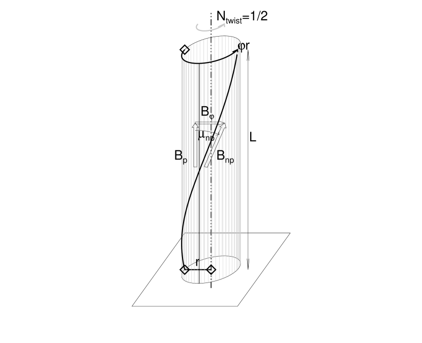
Figure 1: Geometric concept of the vertical-current approximation model of a torsionally twisted flux tube: The potential field component $B_{r}=B_{p}$ is aligned with the flux tube symmetry axis, the nonpotential field component $B_{np}$ follows the torsionally twisted flux tube with a constant misalignment angle $\mu_{np}$, and the azimuthal field component $B_{\varphi}$ is orthogonal to the potential field component $B_{p}$. The twist corresponds to a half turn ($n_{twist}=0.5$) over a flux tube length $L$ at a radius $r$.

where the free energy $B_{f}({\bf r})$ is given here by the azimuthal magnetic field component, i.e., $B_{f}({\bf r})=B_{\varphi}({\bf r})$, in the framework of spherical coordinates ${\bf B}=(B_{r},B_{\varphi},B_{\theta})$. The integration over the 3-D volume renders the total magnetic energy in a flare or an active region. The geometric concept of a torsionally twisted flux tube is depicted in Fig. 1. Eq. (1) reminds us of the Pythagorean geometric relationship in an orthogonal triangle with sides $B_{np}$, $B_{p}$, and $B_{\varphi}$. The radial (potential) field direction $B_{p}$ is orthogonal to the azimuthal (twisting) field component $B_{\varphi}$, as visualized in Fig. 1, so that the sum of the squared sides yield,

$$B_{np}^{2}({\bf r)}=B_{p}^{2}({\bf r})+B_{\varphi}^{2}({\bf r})\ .$$ (2)

consistent with the sum of energies in Eq. (1).

We can now parameterize torsional oscillations in a helically twisted (straight) flux tube. In this geometric concept, the potential field and the azimuthal component can always be decoupled, and thus the potential field can be kept stationary, while the azimuthal component can oscillate independently, so that the vector Eq. (2) reads as,

$$E_{np}(t)=E_{p}+E_{\varphi}(t)\ .$$ (3)

We can model the time variation of the free energy of a torsionally twisted flux tube with a sine function,

$$E_{f}(t)=E_{\varphi}(t)=E_{f0}\ \sin{\left({2\pi(t-t_{0})\over P}\right)}\ ,$$ (4)

where the time evolution of the free energy $E_{f}(t)$ or $E_{\varphi}(t)$ is a direct observable in our data analysis.

2.2 The Magnetic Field

We use a nonlinear force-free field (NLFFF) code that satisfies the divergence-free condition

$$\nabla\cdot{\bf B}=0\ ,$$ (5)

and the force-freeness condition,

$$\nabla\times{\bf B}=\alpha({\bf r}){\bf B}=4\pi{\bf j}\ ,$$ (6)

where $\alpha({\bf r})$ represents a scalar function that depends on the position ${\bf r}$, but is constant along a magnetic field line, and ${\bf j}$ represents the current density. Three different types of magnetic fields are generally considered in applications to the solar corona: (i) a potential field (PF) where the $\alpha$-parameter vanishes $(\alpha=0)$, (ii) a linear force-free field (LFFF) $(\alpha=const)$, and (iii) a nonlinear force-free field (NLFFF) with a spatially varying $\alpha({\bf r})\neq 0$.

Previously we developed a nonlinear force-free field code that models the 3-D coronal magnetic field in (flaring or non-flaring) active regions, which we call the Vertical-Current Approximation (VCA-NLFFF) code (Aschwanden and Sandman 2010; Sandman et al. 2009; Sandman and Aschwanden 2011; Aschwanden et al. 2012, 2014a, 2014b, 2015, 2016c, 2018 Aschwanden 2013a, 2013b, 2013c, 2015, 2016, 2019b, 2019c; Aschwanden and Malanushenko 2013; Warren et al. 2018). It has an advantage over other NLFFF codes by including the magnetic field of (automatically traced) coronal loops, while standard NLFFF codes use the transverse field components in the non-forcefree photosphere, which is inadequate to reconstruct the force-free coronal magnetic field (DeRosa et al. 2009). The inclusion of coronal field directions is accomplished by automated tracing of 2D-projected loop structures in EUV images, such as from AIA/SDO.

An approximate solution of the divergence-free and force-free magnetic field can be derived analytically. The third version of the (VCA3-NLFFF) code is described in more detail in Aschwanden (2019c), while the latest version of this forward-fitting (VCA4-NLFFF) code is described in more detail in Appendix A.

The analytical solution of the force-free magnetic field of a buried unipolar magnetic charge is (Aschwanden 2019c),

$$B_{r}(r,\theta)=B_{0}\left({d^{2}\over r^{2}}\right){1\over(1+b^{2}r^{2}\sin^{2}{\theta})}\ ,$$ (7)

$$B_{\varphi}(r,\theta)=B_{0}\left({d^{2}\over r^{2}}\right){br\sin{\theta}\over(1+b^{2}r^{2}\sin^{2}{\theta})}\ ,$$ (8)

$$B_{\theta}(r,\theta)=B_{0}\left({d^{2}\over r^{2}}\right){b^{2}r^{2}\sin^{3}(\theta)\over(1+b^{2}r^{2}\sin^{2}\theta)}{1\over\cos\theta}\ ,$$ (9)

$$\alpha(r,\theta)\approx{2b\cos{\theta}\over(1+b^{2}r^{2}\sin^{2}{\theta})}\ .$$ (10)

where the constant $b$ is defined in terms of the number of full twisting turns $n_{twist}$ over the loop length $L$, i.e., $b=2\pi n_{twist}/L$. The azimuthal field component $B_{\varphi}(r,\theta)$ (Eq. 8) is most suitable to measure torsional oscillations of a twisted magnetic field directly (Eq. 4).

The total non-potential magnetic field from an arbitrary number of $m=1,...,n_{m}$ unipolar magnetic charges can be approximately obtained from the vector sum of all magnetic components $m$,

$${\bf B}({\bf x})=\sum_{m=1}^{N_{\rm m}}{\bf B}_{m}({\bf x})\ ,$$ (11)

where the vector components ${\bf B}_{m}=(B_{x,m},B_{y,m},B_{z,m})$ of the non-potential field of a magnetic charge $m$ have to be transformed into the same coordinate system. The resulting model can be parameterized with $5n_{m}$ free parameters $(B_{m},x_{m},y_{m},z_{m},\alpha_{m})$ per magnetic charge for a non-potential field, or with $4n_{m}$ free parameters for a potential field (with $\alpha_{m}=0$). This new analytical solution is of second-order accuracy in the divergence-freeness condition, and of third-order accuracy in the force-freeness condition (Aschwanden 2019c).

3 OBSERVATIONS AND DATA ANALYSIS

3.1 Data Sets

Our goal is to study the time evolution of the free energy $E_{f}(t)$ and related energy dissipation mechanisms during solar flares. For this purpose we use the line-of-sight magnetograms $B_{z}(x,y)$ from the Helioseismic and Magnetic Imager (HMI) (Scherrer et al. 2012), and EUV images from the Atmospheric Imaging Assembly (AIA) (Lemen et al. 2012), both instruments onboard the Solar Dynamics Observatory (SDO) (Pesnell et al. 2011). We analyze the same subset of 11 GOES X-class flares presented in previous papers (Aschwanden et al. 2014a; Aschwanden 2019c), which represents all X-class flares observed with the SDO during the first 3.5 years of the mission (2010 June 1 to 2014 January 31). This selection of events has a heliographic longitude range of $[-45^{\circ},+45^{\circ}]$, for which magnetic field modeling can be faciliated without too severe foreshortening effects near the solar limb. We use the 45-s line-of-sight magnetograms from HMI/SDO. We make use of all coronal EUV channels of AIA/SDO (in the six wavelengths 94, 131, 171, 193, 211, 335 Å), which are sensitive to strong iron lines (Fe VIII, IX, XII, XIV, XVI, XVIII, XXI, XXIV) in the temperature range of $T\approx 0.6-16$ MK. The spatial resolution is $\approx 1.6"$ (0.6” pixels) for AIA, and the pixel size of HMI is 0.5”. The coronal magnetic field is modeled by using the line-of-sight magnetogram $B_{z}(x,y)$ from HMI and (automatically detected) projected loop coordinates $[x(s),y(s)]$ in each EUV wavelength of AIA. A full 3-D magnetic field model ${\bf B}(x,y,z)$ is computed for each time interval and flare with a cadence of 3 minutes, where the total duration of a flare is defined by the GOES flare start and end times, including a margin of 30 minutes before and after each flare. The size of the computation box amounts to an area with a width and length of 0.35 solar radius in the plane-of-sky, and an altitude range of $h=0.003-0.25$ solar radius. The total number of analyzed data includes 300 HMI images and 3538 AIA images.

3.2 Loop Decimation

The automated tracing of loop segments in EUV images from AIA yields typically $\approx 500$ loop segments in 6 different coronal wavelengths per time frame, which may contain a sizable number of inaccurately traced loops, resulting from confusion by over- and under-lying structures along the line-of-sight, or by contamination from moss-like features (De Pontieu et al. 1999). It is therefore recommendable to filter out such spurious loop structures that exhibit a large persistent misalignment angle during subsequent iterations in our forward-fitting VCA4-NLFFF procedure. We define a threshold for the number of loops used in the fitting of the VCA4-NLFFF code, expressed by an elimination ratio $q_{elim}=n_{elim}/n_{det}$ of the number $n_{elim}$ of eliminated loops as a fraction of all detected $n_{det}$ loops. The selection of eliminated loops is made by sorting of their misalignment angles $\mu_{3}$ (between the observed loop direction and the theoretical magnetic field line direction) at each iterative time step of our forward-fitting (VCA4-NLFFF) code. At the first iteration step, the theoretical model is given by the potential field, while the theoretical model converges towards a divergence-free and force-free solution in the later iteration steps. A high elimination rate (say $q_{elim}=0.9$) yields a small number of fitted loops, which results into a smaller misalignment angle $\mu_{3}$, while a low elimination rate (say $q_{elim}=0.6$) yields larger statistics, but also larger misaligment angles. The choice of the loop elimination rate is therefore a trade-off between high accuracy and statistical robustness. Consequently, the variation of the loop elimination rate yields also a measure of the uncertainty of the derived free energies $E_{f}(t)$.

3.3 Example of an Analyzed Event

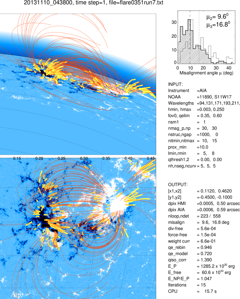
Figure 2: HMI magnetogram (blue), automatically traced coronal loop segments in AIA (yellow), and magnetic field lines computed with the VCA4-NLFFF code (red curves) for flare event # 351, observed on 2013-Nov-10 04:38:00 UT. The line-of-sight magnetogram $B_{z}(x,y)$ is shown (bottom panel), as well as rotated to the north by $90^{\circ}$ (top panel). Histograms of misalignment angles are shown for the 2-D projected ($\mu_{2}=9.6^{\circ}$) and the 3-D reconstructed ($\mu_{3}=16.8^{\circ}$) loop directions with respect to the VCA4-NLFFF magnetic field model.

An example of an analyzed event is given in Fig. 2, where also the control parameters of the VCA4-NLFFF algorithm are listed. First, a HMI magnetogram (blue images in Fig. 2) is decomposed into $n_{m}=30$ unipolar sources, which yield the photospheric magnetic field values $B_{m}$, the coordinates of the unipolar magnetic charges $(x_{m},y_{m},z_{m})$ below the photosphere, and the nonlinear $\alpha_{m}$-parameters for each of the $m=1,...,30$ magnetic charges. In the second task, a total of $n_{det}=558$ loop structures are detected (yellow curves in Fig. 2), while for each loop structure the projected coordinates $[x(s_{i}),y(s_{i})]$ along the curvi-linear loop geometry are measured and interpolated in $n_{s}=5$ segments along the loop trajectory $s_{i},\ i=1,...,n_{s}$. The line-of-sight coordinate $[z(s_{i}]$ is then estimated from 50 parabolically curved loop geometries (for each loop), where the best-fitting geometry that has the smallest misalignment angle $\mu_{3}$ is chosen for further iterations of the VCA4-NLFFF fitting process. The iterative forward-fitting varies both the $n_{m}=30$ $\alpha$-parameters and the $n_{loop}=223$ loop geometries, until it converges to a minimum misalignment angle $\mu_{2}$. The run shown in Fig. 2 reached a minimized misalignment angle of $\mu_{2}=9.6^{\circ}$ after $n_{iter}=15$ iteration steps. A set of magnetic field lines is shown in Fig. 2 (red curves), where all field lines intersect with the midpoints of the observed loop segments (yellow curves). The full procedure is then repeated for every time step with a cadence of 3 minutes, which yields the time evolution of the free energy $E_{f}(t)$ as defined in Eq. (1). Moreover, we repeated each run four times with different loop elimination factors, i.e., $q_{elim}=0.6,0.7,0.8,0.9$, in order to estimate uncertainties of the free energy $E_{f}(t)$.

4 RESULTS

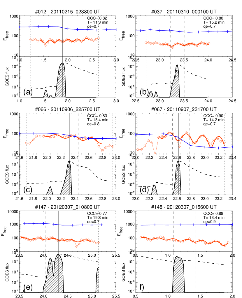
Figure 3: Time evolution of the free energy $E_{f}(t)$ (red diamonds), fit of oscillatory function (red thick curve), free energy evolution from Wiegelmann NLFFF code (blue curves), GOES light curves at 1-8 Å (dashed black curves), and time derivative of GOES light curve (hashed areas). The flare start and end times (dashed vertical lines) according to NOAA.

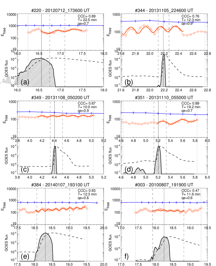
Figure 4: Similar representation as in Fig. 4 for 5 more X-ray flares.

The results of our analysis is the time evolution of the free energy, $E_{f}(t)$, which is shown for 11 GOES X-class flares in Figs. 3 and 4 (red diamonds) on a logarithmic scale, and in Fig. 5 on a linear scale (diamonds), while the best-fit parameters are listed in Table 1. For comparison we show also the free energy $E_{f}^{W}(t)$ obtained from the Wiegelmann nonlinear force-free field (W-NLFFF) code as calculated earlier (Figs. 6 and 7 in Aschwanden 2019c), the GOES 1-8 Å flux (dashed curves in Figs. 3 and 4), and the GOES time derivative (hatched areas in Figs. 3 and 4.) Note that we calculated VCA4-NLFFF solutions with a cadence of 3 minutes, while the used Wiegelmann NLFFF solutions have a cadence of 12 minutes.

4.1 Free Energy Oscillations

The most striking result of this study is the discovery of oscillations in the free energy of each of the 11 analyzed large (GOES X-class) flares, as it can be seen by eye in Figs. 3, 4, and 5. This data set of 11 flares contains between $n_{p}=1$ and $n_{p}=4$ pulses during the duration of a flare (Table 1).

Fitting a sinusoidal function with a linear trend,

$$E_{f}(t)^{osc}=A_{0}+A_{1}(t-t_{0})+A_{2}\sin{\left(2\pi(t-t_{0})\over P\right)}\ ,$$ (12)

to the observed time profiles of the free energy (Eq. 4) we find oscillations periods in the range of $P=(10.0,...,22.5)$ minutes, amplitudes of $A_{0}=(0.34,...,2.29)\times 10^{30}$ erg, linear gradients of $A_{1}=(-0.50,...,2.78)\times 10^{30}$ erg hrs^-1, oscillation amplitudes of $|A_{2}|=(0.04,...,0.73)\times 10^{30}$ erg, and modulation depths of $M=|A_{2}/A_{0}|=0.09,...,0.42$, as listed in Table 1. The time intervals during which we fit the sinusoidal function are chosen include at least the flare duration (given by the NOAA flare start times $t_{s}$ and end times $t_{e}$, marked with vertical dashed lines in Figs. 3, 4, and 5), and are extended by margins of up to $\pm 0.5$ hrs. A measure of the adequacy of fits is given by the cross-correlation coefficient

$$CCC={\sum_{i}E_{f}^{osc}(t_{i})E_{f}^{obs}(t_{i})\over\sum_{i}E_{f}^{osc}(t_{i})\times\sum_{i}E_{f}^{obs}(t_{i})}\ ,$$ (13)

between the observed $E_{f}^{obs}(t)$ and the best-fit oscillatory function $E_{f}^{osc}(t)$ (Eq. 12), which all are found in the range of $CCC=0.67-0.90$, with a mean value of $CCC=0.83\pm 0.07$. Consequently, the oscillations are significant and highly correlated with all observed data.

As a test of the 11 $>X1.0$ class flare events analyzed here, we investigate also a small flare event #003, which is of GOES class M, shown in Fig. 4f. This event shows a poor cross-correlation coefficient ($CCC=0.47$), probably affected by higher noise in the free energy solutions than in the case of X-class flares.

In order to separate valid coronal loops from spurious detections we repeated the fits for four different elimination thresholds of ($q_{elim}=0.6,0.7,0.8,0.9$) and selected those loop data sets that yield the highest cross-correlation coefficient. We list in Table 1 also the median misalinment angles $\mu_{2}=5.3^{\circ}-14.7^{\circ}$ of the best-fitting VCA4-NLFFF magnetic field models, which represents a goodness-of-fit criterion of the theoretical magnetic field model (Section 2).

4.2 Phase Speed

Let us estimate the phase speed of a hypothetical wave that produces torsional oscillations, as depicted in Fig. 7 (left). The example of flare #351 shown in Fig. 2 has a field-of-view of $x_{fov}=0.35$ solar radius and the separation between the western and eastern sunspots amounts to $2R\approx 130$ Mm, where we approximate the length $L$ of the field line by a semi-circular geometry, $L=\pi R\approx 200$ Mm. The propagation distance $L$ corresponds to the length of the mean field line between the two footpoint nodes of the dominant dipole configuration in each flare. We measured these length scales and find a mean of $L=135\pm 35$ Mm (Table 1). Based on the assumption of the oscillations in the free energy $E_{f}(t)$ or azimuthal field component $B_{f}(t)$ to be in the fundamental standing mode, i.e., with the wavelength equal to $2L$ and the wave period $P_{obs}$ being the time scale between two subsequent peaks, the phase speed $v_{phase}$ can be estimated as,

$$v_{ph}={2L\over P_{obs}}\approx 315\pm 120\quad({\rm km}\ {\rm s}^{-1})\ .$$ (14)

The values of the lengths $L$, the time periods $P_{obs}$, and the phase speeds $v_{ph}$ are listed for the analyzed 11 flare events in Table 1.

4.3 Evolutionary Trends of Free Energy

Besides the oscillatory motion of the free energy $E_{f}(t)$, we note also a linear trend $A_{1}\neq 0$ in all flares,

$$E_{f}(t)^{lin}=A_{0}+A_{1}(t-t_{0})\ ,$$ (15)

which is positive in 7 cases, and negative in 4 cases (Table 1). The signs of the linear trends $A_{1}$ in the free energy $E_{\varphi}(t)$ bear important diagnostics whether the free energy is dissipated (if negative) or if new emerging flux (if positive) is occurring. By multiplying the linear energy trend with the flare duration $D$, we obtain the net increase or decrease of free energy during the flares,

$$\Delta E_{f}=A_{1}\ D\ .$$ (16)

Note that the time evolution of the free energy $E_{f}(t)$ in the Wiegelmann (W-NLFFF) code shows a significant decrease in 8 flare events (Figs. 3 and 4, blue curves), but stays constant in the other 3 investigated cases (flares #148, 220, 384). None of the flares exhibits oscillations when using the Wiegelmann (W-NLFFF) code, which is a result of the pre-processing and smoothing technique (which suppresses torque; Wiegelmann et al. 2006), as well as due to the lower cadence of 12 minutes available here.

The time evolution of the free energy $E_{f}(t)$ oscillations reveal that oscillations are detected during the entire analyzed time window of $[t_{s}-0.5,t_{e}+0.5]$ hrs in two cases (#147, #148), which would be expected in the case of an omni-present instrumental effect. However, the beginning of the oscillation period is detected in 8 cases (events #12, #37, #66, #67, #220, #349, #351, and #384, see Fig. 5), which clearly demonstrates the solar origin of the triggered oscillations, rather than being an omni-present instrumental effect.

4.4 Comparison of NLFFF Codes

The comparison with the Wiegelmann NLFFF code shows some intriguing differences. The absolute value of the free energy matches those of the Wiegelmann NLFFF code only in 2 cases out of the 11 events (flares #66 and $67 in Figs. 3c and 3d), but is otherwise always lower, i.e., $E_{f}(t)\leq E_{f}^{W}(t)$, up to an order of magnitude (e.g., flare #147 in Fig. 3e). The reason for this discrepancy is not understood at this time. The most likely reason is that no coronal loops have been detected (or they have been eliminated) in some compact high magnetic field regions, using our automated loop tracing code, especially in the core of the active region, where “moss strucutres” interfere with the tracing of overlying loops. However, we have to be aware that the free energy is a small difference of two large quantities, so that the relative uncertainty of free energy measurements is much larger than for the potential or nonpotential field components. Typically, the free energy amounts to $\approx 1\%$ to 10% of the nonpotential energy, and thus an order of magnitude difference in the free energy corresponds only to 1% to 10% of the nonpotential energy. In a previous study we found that both the potential energy and nonpotential energy agree within $E_{p}/E_{p}^{W}=0.8\pm 0.2$ and $E_{np}/E_{np}^{W}=0.8\pm 0.2$ with the Wiegelmann NLFFF code (see Fig. 6 in Aschwanden 2016). Alternatively, the pre-processing of the magnetogram data carried out with the Wiegelmann NLFFF code (Wiegelmann et al. 2006) could possibly over-estimate the free energy (Yan Xu, private communication).

5 INTERPRETATION AND DISCUSSION

5.1 Instrumental Oscillatory Effects

Since these observations report for the first time oscillations in the free (magnetic) energy of solar flares, we discuss first possible effects of instrumental origin. The range of observed oscillations (in 11 flare events) cover the range of $P\approx 10-22$ min and have a mean and standard deviation of

$$P_{obs}=15.1\pm 3.9\ ({\rm min})\ .$$ (17)

Since the SDO spacecraft is positioned in the Lagrangian point L1, there are no eclipsing time intervals of the spacecraft orbit that could modulate the observed flux.

Since the Sun is rotating, any tracking of a particular heliographic position of a solar flare or an active region needs to be interpolated between two pixels, which could possibly introduce a pixel-step modulation. We estimate the time scale of a pixel shift based on the synodic solar rotation rate,

$$\Delta t_{pix}=P_{syn}\left({\Delta x_{pix}\over 2\pi R_{\odot}}\right)\approx 3.2\ ({\rm min})\ ,$$ (18)

which amounts for a synodic rotation time of $P_{syn}=27.27$ days, an HMI pixel size of $\Delta x_{pix}=0.5\hbox{${}^{\prime\prime}$}$, and an average solar radius of $R_{\odot}\approx 960\hbox{${}^{\prime\prime}$}$, to a time interval of $\Delta t_{pix}=3.2$ min for HMI, or $\Delta t_{pix}=3.9$ min for AIA pixels. The beat frequency between the two instruments amounts to a time scale of

$$P_{beat}=\left[{1\over P_{HMI}}-{1\over P_{AIA}}\right]^{-1}=\left[{1\over 3.2{\rm(min)}}-{1\over 3.9{\rm(min)}}\right]^{-1}=17.8\ {\rm(min)}\ .$$ (19)

Although the beat frequency is close to the frequency of the observed mean oscillation period (Eq. 17), sub-pixel variations of the sensitivity (or modulation transfer function) of AIA are unlikely to explain the observed oscillations, since the width of the point spread function is substantially wider ($1.5\hbox{${}^{\prime\prime}$}$) than the pixel size ($0.6\hbox{${}^{\prime\prime}$}$) (Lemen et al. 2012; Boerner et al. 2012; Grigis et al. 2012). The point-spread function may also imply a slight sub-pixel variation of the sensitivity of CCD pixels (between the pixel center and pixel edge). We calculated this variation by pixel-wise superposition of point-spread functions and found an inter-pixel variation of $\;\buildrel<\over{\scriptstyle\sim}\;$3%. Moreover, the rms variation in the AIA flat-field is found to be of order 2% (Boerner et al. 2012). The point-spread function was also measured during a lunar transit, finding that the PSF of AIA/SDO is better by a factor of two than the EUV telescope onboard of TRACE (Poduval et al. 2013). In summary, no instrumental effect is known from AIA or HMI that could modulate the observed free energy evolution $E_{f}(t)$ with periods of $P\approx 10-20$ min (James Lemen, Paul Boerner, Mark Cheung, Wei Liu; private communication).

Incidentally we did choose a cadence of 3 min for the AIA images with the VCA4-NLFFF code, while a cadence of 12 min is available from the W-NLFFF code using HMI data (Aschwanden 2019c). The cadence of 12 min is close to the mean observed period of $P_{obs}=15.1\pm 3.9$ min, and thus the observed oscillations are fully resolved with the 3-minute cadence of the VCA4-NLFFF code only, while they are not resolved with the available data from the W-NLFFF code (Figs. 3 and 4).

5.2 Torsional Oscillations of Alfvénic MHD Waves

After we ruled out instrumental effects, we turn to a physical model for the interpretation of the observed oscillations. Since the free energy is related to the azimuthal magnetic field component by definition, $B_{f}(t)=B_{\varphi}(t)$, in our vertical-current approximation model (i.e., VCA4-NLFFF code), we can interpret the observed pulsations in terms of torsional oscillations of a helically twisted magnetic field structure in the flaring active region. The overall magnetic field structure in an active region can often be approximated with a bipolar structure in approximate East-West direction, modeled with two unipolar magnetic charges of opposite magnetic polarity. If this bipolar structure is near to a potential field configuration, the magnetic field lines connect the leading sunspot with the trailing region of opposite magnetic polarity along the most direct dipolar field lines, while these field lines become helically twisted like a sigmoid in strongly nonpotential field configurations (Aschwanden 2004, 2019a). In reality, the magnetic field structure consists of many more smaller dipoles and quadrupoles, but the overall bipolar structure is dominant. A good example is shown in Fig. 2, showing a major dipolar configuration between the western positive magnetic polarity (leading sunspot) and the eastern negative magentic polarity (trailing plage).

For the interpretation of the wave type we may consider the MHD modes predicted in a standard thin fluxtube model, which includes slow-mode, fast-mode MHD waves, and torsional Alfvén waves (Edwin and Roberts 1983; Robert et al. 1984). Our estimate of the phase speed yields a mean value of $v_{phase}=315\pm 120$ km s^-1 (Section 4.2 and Table 1), which is inbetween the phase speed expected for slow-mode MHD waves, defined by the sound speed $c_{s}=150\sqrt{{T_{e}/1\ {\rm MK)}}}$ (km s^-1), and the torsional Alfvén waves, defined by the Alfvén speed $v_{A}=2.18\times 10^{6}B/\sqrt{n_{e}}$ (km s^-1). Typical values for the Alfvén speed in active regions are of order $v_{A}\approx 1000$ km s^-1 (using $B\approx 15$ G and $n_{e}\approx 10^{9}$ cm^-3), while the Alfvén speeds in flaring loops have a lower value of $v_{A}\approx 300$ km s^-1, for instance assuming an order of magnitude higher densities than the surrounding backgroun corona ($n_{e}\approx 10^{10}$ cm^-3). Therefore, our measured phase speed, $v_{phase}=315\pm 120$ km s^-1 is consistent with torsional Alfvén waves in flare loops with enhanced electron densities. On the other side, (fast) kink-mode periods have been found to have shorter periods ($P_{kink}=5.4\pm 2.3$ min; Aschwanden et al. 2002), while slow-mode periods were found to have similar periods, ($P_{slow}=17.6\pm 5.4$ min; Wang et al. 2003), than measured here, but oscillation periods depend on both the loop lengths $L$ an the phase speed $v_{phase}$ of the MHD waves ($P\approx 2L/v_{phase}$), and thus do not provide an independent diagnostic of the wave type.

Alternatively, the phase speed would be consistent with slow-mode MHD waves also, if the temperature in the oscillating loops amounts to $T_{e}=4$ MK, yielding $v_{phase}\approx c_{s}\approx 300$ km s^-1, but such an interpretation would face a number of inconsistencies: i) Theoretically, the coupling between torsional Alfvénic oscillations and slow-mode waves is very weak in the low plasma-$\beta$ regions of the solar corona (De Moortel et al. 2004; Zaqarashvili et al. 2006; Afanashvili et al. 2015); (ii) The restoring force in slow-mode MHD oscillations is mainly the plasma pressure, rather than the Lorentz force in the case of torsional Alfvénic oscillations. If slow-mode oscillations are the case here, some correlation between the radiated soft X-ray flux and free energy oscillations would be expected, which is not obvious in the GOES data and free energy time profiles shown in Figs. 3 and 4; and (iii) The damping of slow-mode oscillations has been found to be strong (Wang et al. 2003a, 2003b) due to the conductive losses from hot postflare loops, opposed to the mostly decay-less amplitudes observed here (Fig. 5).

A further test of the hypothesis of torsional waves is the self-consistency of the time evolution of the various magnetic energies. We show the time evolution of the potential energy $E_{p}(t)$ and the free energy $E_{f}(t)$ in Fig. 6, while the evolution of the free energy $E_{f}(t)$ is shown in Fig. 5. The potential energy is uncorrelated to the free energy, as the cross-correlation coefficients in Fig. 6 demonstrate, with a mean and standard deviation of $CCC=0.26\pm 0.16$. This uncorrelatedness is expected, because the azimuthal magnetic field component is orthogonal to the radial magnetic potential field component, i.e., $B_{\varphi}(t)\perp B_{r}$ (Fig. 7 left). In contrast, if the potential energy and free energy would be correlated, the azimuthal energy would vary proportionally with the potential field energy, which could only be explained by field-aligned current oscillations (Fig. 7 right). At the same time, the uncorrelatedness of the potential energy and free energy rules out instrumental effects as the source of the observed oscillations.

Theoretically, the dispersion relation and coupling of wave modes in twisted magnetic flux tubes is treated in Chapter 7 of Roberts (2019). The process of resonant energy transfer from torsional oscillations into acoustic waves has been modeled also (Zaqarashvili 2003; Zaqarashvili and Murawski 2007). Further analytical models and numerical simulations of torsional waves in flux tubes and the generation of compressible flows have been carried out in a number of studies (e.g., Copil et al. 2008, 2010; Vasheghani-Farahani et al. 2010, 2011), which may explain swirling motions, tornadoes, and helical spirals in twisted solar structures (Mozafari Ghoraba and Vasheghani-Farahani 2018; Vasheghani-Farahani et al. 2017).

5.3 The Lorentz Force

Torsional oscillation in magnetic flux tubes are usually referred to the oscillations with the Lorentz force as a restoring force. In the observations presented here, the oscillation of the azimuthal magnetic field component $\Delta B_{\varphi}^{2}(t)\propto\Delta E_{f}(t)\propto\sin{(t)}$ appears to cause small-amplitude torsional oscillations with a Lorentz force acting as a counter balance in restoring the toroidal motion. Since this torsional system exhibits a non-constant motion, the Lorentz force cannot be zero, and thus the magnetic system cannot be force-free. This appears to be in contrast to the near-forcefree solutions attempted with the vertical-current approximation (VCA4-NLFFF) code. This code is designed to converge to a divergence-free and force-free solution for every time step. Obviously our solutions of the VCA4-NLFFF code are not exactly force-free, but oscillate in synchrony with the Lorentz force driver. In fact, the time evolution shown in Fig. 6 explicitly demonstrates that the magnetic potential field is almost constant and thus force-free, while the free energy oscillates and thus is non-forcefree. The degree of non-force-freeness is quantified with the 2-D and 3-D misalignment angles (typically $\mu_{2}\approx 10^{\circ}-20^{\circ}$ in our study). One would expect that an equilibrium situation would occur when the small-amplitude torsional oscillations decay to a minimum energy state, with both the potential field and the free energy becoming constant, while the Lorentz forces converge to zero.

5.4 Measuring Torsional Oscillations in the Corona

Torsional oscillations of sunspots, which harbour the footpoints of many active region loops have been observed to rotate on much longer time scales. For instance, rotational periods in the range of $P\approx 2-8$ days were reported (Gopasyuk and Kosovichev 2011; Grinon-Marin et al. 2017), and thus cannot be considered as the driver of the azimuthal oscillations observed here (with $P\approx 10-22$ min), although they are located at the right place.

The torsional motion of coronal loops is difficult to measure, because we can observe their 2-D projected motion only, unless we attempt a 3-D reconstruction by stereoscopic means or by 3-D magnetic field modeling. Alternatively, it was proposed to detect periodical broadenings of spectral lines that result from periodic azimuthal velocities (Zaqarashvili 2003; Zaqarashvili and Murawski 2007). Ubiquitous torsional motions in type II spicules were identified from spectral line velocities (of order 25-30 km s^-1), in particular in the outer red and blue wings of chromospheric lines, besides the field-aligned flows ($\approx 50-100$ km s^-1) and swaying motions ($15-20$ km s^-1) (De Pontieu et al. 2012; Sekse et al. 2013). However, these velocities are generally smaller than those measured here.

5.5 Damping of Torsional Waves

In the time evolution of oscillatory motion shown in Fig. 5 we note that most oscillation events do not exhibit a detectable degree of wave damping, which creates a new puzzle. Most MHD oscillation modes exhibit relatively short damping times, in the order of 1-4 pulses (Aschwanden et al. 1999; Nakariakov et al. 1999), while we find $n_{p}=1-4$ pulses per flare duration here without damping (Table 1). One damping mechanism is resonant absorption, which transfers energy from the fast kink mode to Alfvénic azimuthal oscillations within the inhomogeneous layer (Ruderman and Roberts 2002). However, there also cases with no detectable damping in the post-flare phase, called decay-less oscillations (Anfinogentov et al. 2013; Nistico et al. 2013). The damping due to resonant absorption (acting in the inhomogeneous regions of a flux tube where energy is transferred from the kink mode to Alfvén azimuthal oscillations) is analytically treated in Ruderman and Robers (2002), who suggest that those loops with density inhomogeneities on a small scale (compared with the loop cross-sectional width) are able to support (observable) coherent oscillations for any length of time, while loops with a smooth cross-sectional density variation do not exhibit pronounced oscillations. An alternative explanation is that torsional waves efficiently modulate gyrosynchrotron emission, which are not subject to radiative and conductive damping and this way can produce stable pulse repetition rates in solar radio pulsation events during flares (Tapping 1983).

6 CONCLUSIONS

Torsional oscillations, which essentially are dynamical systems that have the torque as restoring force, have been invoked in many solar phenomena, such as for the global Hale 11-year solar cycle, oscillatory deviations from the solar differential rotation, meridional circulation, the solar and stellar convection zone, helioseismic measurements of flows in the solar interior, photospheric flux tubes, flows of intergranulary magnetic flux concentrations, sunspot rotations, torsional motions of coronal loops and threads, type II spicules, solar tornadoes, solar radio bursts, and torsional Alfvén waves in the solar wind. Although detailed models of these solar phenomena require different physical mechanisms, the fundamental concept of circular motion with interacting torque is common.

Here we adding a new discovery (to our best knowledge) that exhibits torsional motion in its purest form, because the oscillatory azimuthal rotation can directly be measured from a 3-D magnetic field model in terms of the azimuthal field component $B_{\varphi}(t)$. Moreover, the 3-D magnetic field model has a high degree of observational fidelity, because the divergence-free and force-free magnetic field solution is fitted to the observed coronal loops, which supposedly represent the “true” magnetic field in a low plasma-$\beta$ corona. Traditional NLFFF models extrapolate the coronal field from a non-forcefree photospheric field, after pre-processing of the photospheric boundary. Moreover, the pre-processing is designed to minimize forces and torques, and this way smoothes out any torsional signal. Consequently, torsional oscillations cannot be reconstructed with pre-processed data (besides the insufficient temporal cadence of 12 min used here), and thus have never been detected with traditional NLFFF codes.

Torsional oscillations have been identified here for a complete data set of all investigated 11 (GOES $\geq$X1.0-class) flares, without any selection effects. The identification of torsional oscillations is based on relatively high cross-correlation coefficients ($CCC\approx 0.83\pm 0.07$) between the observed time evolution of the free energy $E_{f}(t)=E_{\varphi}(t)$ with an oscillatory sine function, and the agreement of the mean observed phase speed, $v_{phase}=315\pm 120$ km s^-1, with torsional Alfvénic MHD waves in density-enhanced flare loops. Our interpretation suggests that the torsional wave may couple with the fast-mode MHD wave, rather than with the slow-mode MHD wave. Also, the torsional oscillations are found to be decay-less, similar to some fast kink-mode decay-less events.

Besides the oscillatory motion, the time evolution of the free energy $E_{f}(t)$ shows also a linear trend, which increases or decreases the free energy in a linear fashion. The simple concept that the free energy drops like a step function during the energy dissipation phase of a flare appears to be over-simplified, because we detect multiple pulses, each one accompanied by a rise and decay of the free energy (Aschwanden 2019c). Consequently, we can filter out the oscillatory part and determine the free energy before (at time $t_{s}$) and after a flare (at time $t_{e}$) from the linear trend, i.e., $\Delta E_{f}=E_{f}(t_{s})-E_{f}(t_{e})$, where flare energy dissipation or magnetic flux cancelling occurs when $\Delta E_{f}<0$ is negative, while emergence of new magnetic flux is required when $\Delta E_{f}>0$.

Future studies should investigate whether torsional oscillations occur during large flares only, what the damping mechanism is for decay-less oscillation events, how accurately we can measure and predict the distributions of sound speeds in a flaring active region, how torsional oscillations couple with slow-mode MHD waves, and how torsional oscillation velocities agree with other methods, such as spectral line broadening.

APPENDIX A: The Vertical-Current Approximation Code Version 4 (VCA4-NLFFF)

The Vertical-Current Approximation (Version 4) Nonlinear Force-Free Field (VCA4-NLFFF) code has been improved in a number or ways over the last 6 years, starting from the original definition (Aschwanden 2013a; 2013b; Aschwanden and Malanushenko 2013c), followed by more detailed code descriptions and performance tests (Aschwanden 2016), more accurate analytical solutions in Version 3 (Aschwanden 2019c), and improved iteration schemes in the current Version 4, which are described in this Appendix.

The VCA4-NLFFF code is publicly available in the Solar SoftWare (SSW) package $\$/$SSW/package /mjastereo/idl/ and consists of a sequence of 13 modules, written in Interactive Data Language (IDL), which we describe here in turn, while a tutorial is provided on the webpage http://www.lmsal.com/ $\sim$aschwand /software/nlfff/nlfff$\_$tutorial.pro.

(1) NLFFF$\_$CAT generates an event catalog in form of a time series (defined by the starting time, total duration, and cadence of an event) with heliographic positions that follow the solar rotation. The longitude change $dl/dt$ per time cadence $P_{cad}$ is calculated from the mean synodic rotation rate $P_{syn}=27.2753\times 86400$ s,

$${dl\over dt}=360^{\circ}\ \left({P_{cad}\over P_{syn}}\right)\ .$$

(2) NLFFF$\_$INIT reads the times, wavelengths, and heliographic positions of an event from the catalog file, saves control parameters, and calculates the cartesian coordinates (in units of solar radii from Sun center) for each time step and (quadratic) field-of-view (FOV), centered at the initial heliographic location and following the differential solar rotation. The cartesian coordinate sytem $(x,y,z)$ is centered at Sun center and takes the curvature of the solar surface or photospheric magnetogram automatically into account, with the line-of-sight coordinate $z_{phot}$ of the photosphere defined by

$$z_{phot}(x,y)=\left(r_{phot}^{2}-x^{2}-y^{2}\right)^{1/2}\ ,$$

and the normalization given by the solar radius, $r_{phot}=R_{\odot}=1$.

(3) NLFFF$\_$HMI reads the HMI/SDO magnetogram $B_{z}(x,y)$ and writes an uncompressed FITS file. Note that a scaling factor BSCALE=0.1 has been introduced in the FITS header in recent years, which changes the absolute scaling of the magnetic field by an order of magnitude.

(4) NLFFF$\_$AIA reads AIA/SDO images in up to 8 wavelengths within a time interval of 12 s for every time step (defined by starting time and cadence), and writes uncompressed FITS files for each wavelength.

(5) NLFFF$\_$FOV displays the selected FOV (at coordinates $[x_{1},y_{1},x_{2},y_{2}]$ for the chosen “cut-out” subimage) and caclulates the solar radius and the AIA pixel size from solar ephemerids, which varies by $\approx 10\%$ due to solar distance variation of the Lagrangian point (L1), where the SDO spacecraft is located.

(6) NLFFF$\_$MAGN extracts the line-of-sight magnetogram $B_{z}(x,y)$ within the selected FOV coordinates, and coaligns the FOV image (by shift and rotation) according to the pointing information given in the FITS header. The extracted HMI magnetogram is rebinned to $3\times 3$ HMI pixels, and then a sequential decomposition of the HMI magnetogram into unipolar magnetic charges is carried out. The decomposition yields the 3-D coordinates $(x_{i},y_{i},z_{i}),i=1,...,n_{m}$ of sub-photospheric magnetic charges that are obtained by fitting the local potential field of a unipolar magnetic charge (which decreases with the squared distance, $B(r)\propto r^{-2}$). The iterative algorithm, which starts with the largest sunspot in the FOV and fits progressively smaller magnetic field concentrations, is decribed in more detail in Aschwanden and Sandman 2010), Aschwanden et al. (2012). Correction factors for re-binning and magnetic field energies are computed also.

(7) NLFFF$\_$TRACING reads AIA images and performs automated tracing of curvi-linear structres, mostly rendering coronal loop segments in the lowest hydrostatic scale height of the corona. The algorithm starts with the brightest structure in an AIA image and traces the local ridge at position $[x(s_{i}),y(s_{i})],i=1,...,n_{s}$ by linear and constant-curvature extrapolation from loop coordinate $s_{i}$ to $s_{i+1}$, where $n_{s}$ is the number of points along a loop, calculated with a step $\Delta s$ corresponding to the pixel size. Some control parameters of this algorithm include the low-pass filter $n_{sm1}$ (which enhances faint loops relative to the local background), the high-pass filter $n_{sm2}=n_{sm1}+2$, which eliminates broad background structures, the minimum loop length $l_{min}$, the minimum curvature radius $r_{min}$, a threshold $q_{thresh1}$ of the intensity image $I(x,t)$, as well as a threshold $q_{thresh2}$ of the filtered image $I(x,t)-smooth[I(x,t)]$, a tolerance gap $n_{gap}$ in tracing along a loop ridge, etc. More detailed descriptions of the automated loop tracing algorithm (also called Oriented Coronal Curved Loop Tracing (OCCULT) are given in Aschwanden et al. (2008; 2013) and Aschwanden (2010).

(8) NLFFF$\_$FIT reads the 2-D loop coordinates $[x(s_{i}),y(s_{i})]$ for each of the multiple-wavelength AIA images, which typically encompasses $n_{loop}\approx 500$ loops. For each loop we test a proxy of the 3-D coordinate $[z(s_{i})]$, which has the geometry of a parabolic loop segment,

$$h_{ijk}(s)=qh_{ijk}-(4\ qh_{ijk})(s-0.5)^{2}\ ,$$

where $s$ is the normalized loop coordinate $0<s_{i}<1,i=0,...,n_{s}$, $qh$ is the normalized height coordinate $0<h_{j}<1,j=0,...,n_{h}$, while $s_{1}=0$ is the first loop footpoint, $s_{2}=s_{i}$ is the second loop footpoint, and $k=0,1$ is the order of the two conjugate footpoints. With the third coordinate $z(s)$,

$$z(s)=\left[(1+h_{ijk}(s))^{2}-x(s)^{2}-y(s)^{2}\right]^{1/2}\ ,$$

we have a full 3-D model $[x(s),y(s),z(s)]$ of a traced loop segment, which converges by selecting those loop geometries $(i,j,k)$ that produce the smallest misalignment angles between the 3-D magnetic field line vectors (Eq. 11) and the observed 3-D loop directions.

An example of these trial loop geometries is given in Fig. 8, Typically, we used $n_{s}=5$ segments per loop and $n_{h}=5$ heights in the range of $h=0.003,...0.25\ R_{\odot}$, which implies $n_{geo}=2n_{s}n_{h}=50$ trial geometries. This proxy assumes that at least one loop footpoint is located near the chromosphere, while the automated tracing detects an arbitrary part of the remaining loop segment. The additional constraint of limiting the height range to the 2-D projected loop length yields improved results, i.e., $|s_{n_{s}}-s_{1}|<(h_{2}-h_{1})$.

The code optimizes three tasks of the full 3-D model of the magnetic field simultaneously: (i) the height model $h(s)$ for each loop, (ii) the nonlinear force-free field parameters $\alpha_{m},m=1,...,n_{m}$ of sub-photospheric magnetic charges that represent the nonpotential field, and (iii) the loop decimation as described in Section 3.2. These three tasks contain a number of recent optimizations that improve the convergence of the VCA4-NLFFF code and are superior to the previous VCA3-NLFFF code. A more stable convergence (based on comparing the solutions in subsequent time steps) was also found by increasing the number of fitted unipolar magnetic charges progressively with the number of iterations. This way, the strongest sunspots dominate the solutions. The optimization of $\alpha$-parameters is done by second-order extrapolation, while it was done by first-order extrapolation in the previous VCA3-NLFFF code. Typically, only 10-20 iteration steps are needed for final convergence, which is measured by the misalignment angle in 3-D ($\mu_{3}$) or 2-D ($\mu_{2}$). The optimization of the entire 3-D model is characterized by a single parameter, the median value of the 3-D misalignment angle ($\mu_{3}$):

$$\mu_{3}({\bf x})=cos^{-1}\left({\bf B}^{model}({\rm x})\cdot{\bf B}^{obs}({\rm x})\over|{\bf B}^{model}({\rm x})|\cdot|{\bf B}^{obs}({\rm x})|\right)\ .$$

(9) NLFFF$\_$FIELD calculates the magnetic field lines of the nonlinear force-free field solution, which is fully constrained by the $5n_{m}$ coefficiencts $(B_{m},x_{m},z_{m},\alpha_{j}),m=1,...,n_{m}$, which typically amounts with $n_{m}=30$ to $5n_{m}=150$ coefficients. We display a graphical rendering of the magnetic field lines by showing magnetic field lines that intersect the midpoint of the observed loops, which allows for a direct inspection of the misalignment angles $\mu_{2}$.

(10) NLFFF$\_$CUBE calculates the nonlinear force-free field $[B_{x}(x,y,z),B_{y}(x,y,z),B_{z}(x,y,z)]$ in a 3-D computation box $(N_{x}\times N_{y}\times N_{z})$ that is given by the photospheric FOV area and a height range of $\Delta h=h_{max}-h_{min}=0.250-0.003$ solar radius. However, it is much more economical to store the $5n_{m}$ coefficients of our model rather than a full 3-D cube with one-pixel resolution.

(11) NLFFF$\_$MERIT calculates figures of merit of a VCA4-NLFFF solution, including measures of the divergence-freeness, force-freeness, and weighted current.

(12) NLFFF$\_$ENERGY calculates the potential energy $E_{p}=\int[B_{p}(x,y,z)^{2}/8\pi]dV$, the nonpotential energy $E_{np}=\int[B_{np}(x,y,z)^{2}/8\pi]dV$, and the free energy $E_{f}=E_{np}-E_{p}$. Correction factors due to rebinning and magnetic modeling are included.

(13) NLFFF$\_$DISP provides renderings of the observed 2-D loops, reconstructed 3-D loops, best-fit field lines of the VCA4-NLFFF solutions, viewed from two orthogonal directions, and histograms of the 2-D and 3-D misalignment angles (for instance see Fig. 2).

References

Afanasyev, A.N. and Nakariakov, V.M. 2015, AA 582, A57.

Anfinogentov, S., Nistico, G., and Nakariakov, V.M. 2013, AA 560, 107.

Antolin, P. and Shibata, K. 2010, ApJ 712, 494.

Aschwanden, M.J., Fletcher, L., Schrijver, C., and Alexander, D. 1999, ApJ 520, 880.

Aschwanden, M.J., DePontieu, B., Schrijver, C.J., and Title, A. 2002, SoPh 206, 99.

Aschwanden, M.J., 2004, Physics of the Solar Corona. An Introduction, Praxis and Springer, Berlin, 216.

Aschwanden, M.J. and Sandman, A.W. 2010, AJ 140, 723

Aschwanden, M.J. 2010, SoPh 262, 399.

Aschwanden, M.J., Wuelser, J.P., Nitta, N.V., Lemen, J.R., Schrijver, C.J., et al. 2012, ApJ 756, 124

Aschwanden, M.J. 2013a, SoPh 287, 323

Aschwanden, M.J. 2013b, SoPh 287, 369

Aschwanden, M.J. 2013c, ApJ 763, 115

Aschwanden, M.J., De Pontieu, B., and Katrukha, A. 2013, Entropy 15, 3007.

Aschwanden, M.J. and Malanushenko, A. 2013, SoPh 287, 345

Aschwanden, M.J., Xu, Y., and Jing J. 2014a, ApJ 797:50.

Aschwanden, M.J., Sun, X.D., and Liu,Y. 2014b, ApJ 785, 34

Aschwanden, M.J. 2015, ApJ 804, L20

Aschwanden, M.J., Schrijver, C.J., and Malanushenko, A. 2015, SoPh 290, 2765

Aschwanden, M.J. 2016, ApJSS 224, 25

Aschwanden, M.J., Reardon, K., and Jess, D. 2016c, ApJ 826, 61

Aschwanden, M.J., Gosic, M., Hurlburt, N.E., and Scullion, E. 2018, ApJ 866, 72

Aschwanden, M.J. 2019a, New Millennium Solar Physics, Springer Nature, Switzerland, Science Library Vol. 458

Aschwanden, M.J. 2019b, ApJ 874, 131

Aschwanden, M.J. 2019c, ApJ 885:49.

Boerner, P., Edwards, C., Lemen, J., Rausch, A., Schrijver, C., Shine, R., Shing, L., Stern, R., et al. 2012, SoPh 275:41.

Chakraborty, S., Choudhuri, S., and Chatterjee, P. 2009, Phys.Rev.Lett. 102, 041102.

Copil, P., Voitenko, Y. and Goossens, M. 2008, AA 478, 921.

Copil, P., Voitenko, Y. and Goossens, M. 2010, AA 510, A17.

Covas, E., Takakov, R., Moss, D., and Tworkowski, A. 2000 AA 360, L21.

Covas, E., Moss, D., and Tavakol, R. 2004, AA 416, 775.

De Moortel, I., Hood, A.W., Gerrard, C.L., and Brooks, S.J. 2004, AA 425, 741.

De Pontieu, B., Berger, T.E., Schrijver, C.J., and Title, A.M. 1999, SoPh 190, 419.

De Pontieu, B., Carlsson, M., Rouppe van der Voort, L.H.M., Rutten, R.J., Hansteen, V.M., and Watanabe, H. 2012, ApJL 752, L12.

DeRosa, M.L., Schrijver, C.J., Barnes, G., Leka,K.D., Lites, B.W., Aschwanden, M.J., Amari, T., Canou,A., et al. 2009, ApJ 696, 1780.

Durney, B.R. 2000, SoPh 196, 1.

Edwin, P.M. and Roberts, B. 1983, SoPh 88, 179.

Fedun, V., Verth, G., Jess, D.B., and Erdelyi, R. 2011, ApJL 740, L46.

Gonzalez-Hernandez, I., Howe, R., Komm, R., and Hill, F., 2010, ApJL 713, L16.

Gopasyuk, S.I. and Kosovichev, A.G. 2011, ApJ 729, 95.

Gosling, J.T., Teh, W.L., and Eriksson, S. 2010, ApJL 719, L36.

Grigis, P., Su, Y., Weber, M., AIA Team 2012, AIA PSF Characterization and Image Deconvolution, Memo Version 2012-Feb-13.

Grinon-Marin, A.B., Socas-Navarro, H., and Centeno, R. 2017, AA 604, A36.

Guerrero, G., Smolarkiewicz, P.K., de Gouveia Dal Pino, E.M. et al. 2016, ApJL 828, L3.

Higginson, A.K. and Lynch, B.J. 2018, ApJ 859, 6.

Howard, R. and LaBonte, B.J. 1980, ApJL 239, L33.

Howe,R., Rempel, M., Christensen-Dalsgaard, J., Hill, F., Komm, R., Larsen, R.M., Schou, J., and Thompson, M.J., 2006, ApJ 649, 1155.

Howe, R., Christensen-Dalsgaard, J., Hill, F., Komm, R., Schou, J., and Thompson, M.J. 2009, ApJL 701, L87.

Howe, R., Christensen-Dalsgaard, J., Hill, F., Komm, R., Larson, T.P., Rempel, M., Schou, J., and Thompson, M.J. 2013, ApJL 767, L20.

Karami, K., and Bahari, K. 2011, Astrophys.Spac.Sci. 333, 463.

Kitchatinov, L.L., Pipin, V.V., Makarov, V.I. and Tlatov, A.G. 1999, SoPh 189, 227.

Kosovichev, A.G. and Pipin, V.V. 2019, ApJL 871, L20.

Lanza, A.F. 2007, AA 471, 1011.

Lemen, J.R., Title, A.M., Akin, D.J., Boerner, P.F., Chou, C., Drake, J.F., Duncan, D.W., Edwards, C.G., et al. 2012, SoPh 275, 17.

Lekshmi, B., Nandy, D., and Antia, H.M. 2018, ApJL 861, 121L.

Link, B. and van Eysden, C.A. 2016, ApJL 823, L1.

Luo, Q.Y., Wei, F.S., and Feng, X.S. 2002, SoPh 205, 39.

Morton, R.J., Ruderman, M.S. and Erdelyi, R. 2011, AA 534, A27.

Mozafari Ghorava A. and Vasheghani-Farahani, S. 2018, ApJ 869, 93.

Murawski, K., Solovev, A., Musielak, Z.E., Srivastava, A.K., and Kraskiewicz, J. 2015, AA 577, A126.

Nakariakov, V.M., Ofman, L., DeLuca, E., Roberts, B., and Davila, J.M. 1999, Science 285, 862.

Narain, U., Agarwal, P., Sharma, R.K., Prasad, L. and Dwivedi, B.N. 2001, SoPh 199, 307.

Nistico, G., Nakariakov, V.M., and Verwichte, E. 2013, AA 552, A57.

Noble, M.W., Musielak, Z.E., and Ulmschneider, P. 2003, AA 409, 1085.

Pesnell, W.D., Thompson, B.J., and Chamberlin, P.C. 2011, SoPh 275, 3.

Petrovay, K. and Forgacs-Dajika, E. 2002, SoPh 205, 39.

Poduval, B., DeForest, C.E., Schmelz, J.T., and Pathak, S. 2013, ApJ 765:144.

Raghav, A.N., Kule, A., Bhaskar, A., Mishra, W., Vichare, G. and Surve S. 2018a, ApJ 860, 26.

Raghav, A.N. and Kule, A. 2018, MNRAS 476, L6.

Rempel, M. 2006, ApJ 647, 662.

Rempel, M. 2007, ApJ 655, 651.

Rempel, M. 2012, ApJL 750, L8.

Roberts, B., Edwin, P.M., and Benz, A.O. 1984, ApJ 279, 857.

Roberts, B. 2019, MHD waves in the solar atmosphere, Cambridge University Press.

Routh, S., Musielak, Z.E., and Hammer, R. 2007, SoPh 246, 133.

Routh, S., Musielak, Z.E., and Hammer, R. 2010, ApJ 709, 1297.

Ruderman, M.S., and Roberts, B. 2002, ApJ 577, 475.

Sakai, J.I., Minamizuka, R., Kawata, R., and Cranmer, N.F. 2001, ApJ 550, 1075.

Sandman, A., Aschwanden, M.J., DeRosa, M., Wuelser, J.P., Alexander,D. 2009, SoPh 259, 1.

Sandman, A.W. and Aschwanden, M.J. 2011, SoPh 270, 503.

Scherrer, P.H., Schou, J., Bush, R.I., Kosovichev, A.G., Bogart, R.S., Hoeksema, J.T., Liu, Y., Duvall, T.L., et al. 2012, SoPh 275, 207.

Sekse, D.H., Rouppe van der Voort, L., De Pontieu, B., and Scullion, E. 2013, ApJ 769, 44.

Shelyag, S. 2015, ApJ 801, 46.

Snow, B., Fedun, V., Gent, F.A., Verth, G., and Erdelyi, R. 2018, ApJ 857, 125.

Soler, R., Terradas, J., Oliver, R., and Ballester, J.L. 2017. ApJ 840, 20.

Soler, R., Terradas, J., Oliver, R., and Ballester, J.L. 2019, ApJ 871, 3.

Spruit, H.C. 2003, SoPh 213, 1.

Strohmayer, T.E. and Watts, A.L. 2006, ApJ 653, 593.

Tapping K.F. 1983, SoPh 87, 177.

Vasheghani-Farahani, S., Nakariakov, V.M., and van Doorsselaere, T. 2010, AA 517, A29.

Vasheghani-Farahani, S., Nakariakov, V.M., van Doorsselaere, T., and Verwichte, E. 2011, AA 526, A80.

Vasheghani-Farahani, S., Ghanbari, E., Chaffari, G., and Safari, H. 2017, AA 599, A19.

Verth, G., Erdelyi, R., and Goossens, M. 2010, ApJ 714, 1637.

Vorontsov, S.V., Christensen-Dalsgaard, J., Schou, J., Strakhov, V.N. and Thompson M.J. 2002, Science, 296, 101.

Wang, T.J., Solanki, S.K., Innes, D.E., et al. 2003a, AA 402, L17.

Wang, T.J., Solanki, S.K., Curdt, W. et al. 2003b, AA 406, 1105.

Warren, H.P., Crump, N.A., Ugarte-Urra,I., Sun,X., Aschwanden,M.J., and Wiegelmann,T. 2018, ApJ 860, 46.

Wiegelmann, T., Inhester, B., and Sakurai, T. 2006, SoPh 233, 215.

Wojcik, D., Murawski, K., Musielak, Z.E., Konkol, P., and Mignone, A. 2017, SoPh 292, 31.

Zaqarashvili, T.V. 2003, AA 399, L15.

Zaqarashvili, T.V., Oliver, R., and Ballester, J.L. 2006, AA 456, L13.

Zaqarashvili, T.V. and Murawski, K. 2007, AA 470, 353.

Zaqarashvili, T.V. and Belvedere, G. 2007, ApJ 663, 553.

Zaqarashvili, T.V., Khodachenko, M.L., and Solar, R. 2013, AA 549, A113.

Zhao, J. and Kosovichev, A.G. 2004, ApJ 603, 776.

Table 1: Results of oscillation analysis (D=flare duration (min), $n_{p}$=number of pulses, CCC=cross-correlation coefficient, $q_{elim}$=fraction of eliminated loop segments; P=Oscillation time period in minutes, $A_{0}$=Initial free energy level ($10^{30}$ erg), $A_{1}$=linear drift of free energy level ($10^{30}$ erg hour^-1), $A_{2}$=Amplitude of oscillation level ($10^{30}$ erg), M=modulation depth, median misalignment angle $\mu_{2}$ of VCA4-NLFFF magnetic field model with respect to observed loop directions), $L$=length of mean field line of dominant dipole, and $v_{phase}$=phase speed along mean field line.

#	Date	Time	D	$n_{p}$	CCC	$q_{elim}$	P	$A_{0}$	$A_{1}$	$A_{2}$	M	$\mu_{2}$	$L$	$v_{phase}$
		[UT]	(min)				(min)					(deg)	(Mm)	(km/s)
12	20110215	023800	24	2	0.82	0.70	11.3	0.51	0.16	-0.09	0.17	9.4	100	300
37	20110310	000100	17	1	0.80	0.70	15.2	0.34	0.08	0.04	0.12	5.3	110	250
66	20110906	225700	15	1	0.83	0.80	15.4	0.86	-0.49	-0.12	0.14	7.2	160	350
67	20110907	231700	15	1	0.90	0.70	14.2	0.82	-0.50	0.28	0.35	7.1	170	400
147	20120307	010800	36	2	0.77	0.70	19.8	1.00	-0.29	0.13	0.13	14.7	130	220
148	20120307	015600	20	2	0.88	0.90	13.4	1.37	-0.47	-0.12	0.09	5.7	70	180
220	20120712	173600	21	1	0.89	0.70	22.5	2.29	2.78	0.73	0.32	14.5	100	150
344	20131105	224600	8	1	0.76	0.90	12.3	1.25	0.42	-0.53	0.42	8.8	130	350
349	20131108	050200	12	1	0.67	0.90	10.0	1.43	0.09	0.12	0.08	13.5	170	570
351	20131110	055000	12	1	0.89	0.70	19.2	0.57	0.54	0.16	0.29	8.0	200	340
384	20140107	193100	56	4	0.83	0.60	12.3	1.43	0.76	0.32	0.22	11.9	130	350
mean			21		0.83		15.1						135	315
			$\pm 14$		$\pm 0.07$		$\pm 3.9$						$\pm 35$	$\pm 120$

Figure 5: The free energy $E_{f}(t)$ as a function of the time is shown for 11 X-class flares (diamonds), together with a fit of a sinusoidal modulation function (thick black curves). The cadence is $\Delta t=3$ minutes, bracketed by the flare start and end times (vertical dashed lines) as defined in GOES data by NOAA.

Figure 6: Time evolution of the potential field energy $E_{p}(t)$ (thick curve with diamonds) and the free energy $E_{f}(t)$ (thin curve with crosses), both normalized to their maximum, the loop elimination ratio $q_{e}$, and cross-correlation coefficient $CCC$. Note that the potential field energy and the free energy are uncorrelated.

Figure 7: Two scenarios of oscillating magnetic field components: torsional oscillations with $B_{p}=const$ and $B_{\varphi}$ oscillating (left side); and field-aligned current oscillations, where the current ${\bf j}\propto(\nabla\times{\bf B})$ oscillates, modulating all components $B_{p}$, $B_{np}$, and $B_{\varphi}$ proportionally (right side).

Figure 8: Trial geometries for segments of loop altitudes $h(s)$.