Predicting Regression Probability Distributions
with Imperfect Data Through Optimal Transformations

Abstract

The goal of regression analysis is to predict the value of a numeric outcome variable $y$ given a vector of joint values of other (predictor) variables $\mathbf{x}$. Usually a particular $\mathbf{x}$–vector does not specify a repeatable value for $y$, but rather a probability distribution of possible $y$–values, $p(y\,|\,\mathbf{x})$. This distribution has a location, scale and shape, all of which can depend on $\mathbf{x}$, and are needed to infer likely values for $y$ given $\mathbf{x}$. Regression methods usually assume that training data $y$-values are perfect numeric realizations from some well behaived $p(y\,|\,\mathbf{x})$. Often actual training data $y$-values are discrete, truncated and/or arbitrary censored. Regression procedures based on an optimal transformation strategy are presented for estimating location, scale and shape of $p(y\,|\,\mathbf{x})$ as general functions of $\mathbf{x}$, in the possible presence of such imperfect training data. In addition, validation diagnostics are presented to ascertain the quality of the solutions.

Keywords: optimal transformations, heteroscedasticity, censoring, ordinal regression, quantile regression

Running title: Predicting regression probability distributions

1 Introduction

In regression analysis one has a system under study with associated attributes or variables. The goal is to estimate the unknown numeric (outcome) value of one of the variables $y$, given the known joint values of other (predictor) variables $\mathbf{x}=$ $(x_{1}\cdot\cdot\cdot,x_{p})$ associated with the system. It is seldom the case that a particular set of $\mathbf{x}$–values gives rise to a unique value for $y$. There are other variables $\mathbf{z}=(z_{1},z_{2},\cdot\cdot\cdot)$ that influence $y$ whose values are neither controlled nor observed. Specifying a particular set of joint values for $\mathbf{x}$ results in a probability distribution of possible $y$–values, $p(y\,|\,\mathbf{x})$, induced by the varying values of $\mathbf{z}$. This distribution has a location $f(\mathbf{x})$, scale $s(\mathbf{x})$ and shape, all of which can depend on $\mathbf{x}$. Using a training data set of previously solved cases $\{y_{i},\mathbf{x}_{i}\}_{i=1}^{N}$ in which both the outcome and predictor variable values are jointly observed, the goal is to produce an estimate $\hat{p}(y\,|\,\mathbf{x})$ of the distribution of $y$ given $\mathbf{x}$.

Most regression procedures explicitly or implicitly approximate $p(y\,|\,\mathbf{x})$ by a generic (usually normal) distribution that is symmetric with constant scale, $s(\mathbf{x})=s$ (homoscedasticity). Only its location function $f(\mathbf{x})$ is estimated from the training data. That estimate $\hat{f}(\mathbf{x})$ can then be used to estimate the presumed constant scale by

$$\hat{s}=\sum_{i\in T}h(|\,y_{i}-\hat{f}(\mathbf{x}_{i})\,|)$$ (1)

on a “test” data set $T$ not used to estimate $\hat{f}(\mathbf{x})$. Here the particular function $h$ employed depends upon the assumed distribution $p(y\,|\,\mathbf{x})$. In this setting a $y$–prediction at a future $\mathbf{x}$–value is taken to be $\hat{f}(\mathbf{x})$ since this is the most likely value of $y$ under a symmetric distribution assumption.  The uncertainty of all predictions is gauged by $\hat{s}$ (1). The value of $\hat{s}$ is often taken to be a measure of the lack-of-quality of the solution, especially in competitions.

The quantity $\hat{s}$ (1) reflects the prediction uncertainty averaged over the marginal distribution of all $\mathbf{x}$–values, $p(\mathbf{x})$. The actual uncertainty for predictions at a particular $\mathbf{x}$ is characterized by $s(\mathbf{x})$, the scale of $p(y\,|\,\mathbf{x})$ corresponding to that $\mathbf{x}$–value. It is seldom the case that this uncertainty is the same or even similar for different $\mathbf{x}$–values. Generally there is substantial variation in the scale $s(\mathbf{x})$ over the distribution of $\mathbf{x}$ (heteroscedasticity). When a predicted value of $y$ is being used in an actual decision making application (rather than in a competition) knowing its corresponding lack–of–accuracy can be important information influencing the decision outcome.

It is important to note that the location $f(\mathbf{x})$ and scale $s(\mathbf{x})$ are characteristics (parameters) of the distribution $p(y\,|\,\mathbf{x})$. In particular, the scale function $s(\mathbf{x})$ represents an “irreducible” error for predictions at $\mathbf{x}$. Obtaining more training data or using more effective learning algorithms cannot reduce this error. They can only reduce the error in the estimated values of the parameters $\hat{f}(\mathbf{x})$ and $\hat{s}(\mathbf{x})$. This latter “reducible”  error is usually much smaller than the irreducible error characterized by the intrinsic scale $s(\mathbf{x})$. The only way to decrease irreducible error is to use a more informative set of predictor variables $\mathbf{x}$.

Along with location and scale, higher moments can also vary with $\mathbf{x}$ giving rise to changing shape of $p(y\,|\,\mathbf{x})$ for different values of $\mathbf{x}$. For example, $p(y\,|\,\mathbf{x})$ may be asymmetric with varying degrees of skewness for different $\mathbf{x}$–values. This will effect inference on likely values of $y$ for a given $\mathbf{x}$.

Almost all regression procedures implicitly assume that the outcome $y$ is a real valued variable with the potential to realize any value for which the marginal distribution of $y$

$$p(y)=\int p(y\,|\,\mathbf{x})\,\,p(\mathbf{x})\,d\mathbf{x}$$

has support. For most hypothesized $p(y\,|\,\mathbf{x})$ used in regression analysis this implies all real values $y\in R$. In many applications, however, this ideal is not realized. Recorded $y$–values may be restricted to a small distinct set with many ties. The tied values themselves may be unknown. Only an order relation among them is recorded (ordinal regression). In other applications, one may only be able to specify (possibly overlapping) intervals that contain each training data $y$–value, rather than the actual value itself (censoring). The specified intervals may be open or closed.

This paper describes an omnibus regression procedure (OmniReg) that can use imperfect training data such as described above to produce estimates of the location $f(\mathbf{x})$, scale $s(\mathbf{x})$ and shape of $p(y\,|\,\mathbf{x})$ as general functions of $\mathbf{x}$. These can be used to assess the distribution of likely values of $y$ for new observations for which only the predictor values $\mathbf{x}$ are known.

Section 2 presents the basic gradient boosting strategy for jointly estimating the location $f(\mathbf{x})$ and scale $s(\mathbf{x})$ of a symmetric $p(y\,|\,\mathbf{x})\,$ in the presence of general censoring of the outcome variable $y$. Section 3 generalizes the procedure by presenting a method for for constructing the optimal transformation of $y$, $g(y)$, on which to perform the corresponding location–scale estimation. Section 4 outlines diagnostic procedures for checking the consistency of derived solutions. Section 5 further generalizes the procedure by incorporating asymmetry, as a function of $\mathbf{x}$, into the transformed $p(g(y)\,|\,\mathbf{x})$ solutions. Illustrations using three publicly available data sets, one censored and two uncensored, are presented in Section 6. Application to ordinal regression, where only an order relation among the $y$-values is observed, is discussed in Section 7. Connections of this method to other related techniques are discussed in Section 8. Section 9 outlines the use of the derived distribution estimates $\hat{p}(y\,|\,\mathbf{x})$ for point prediction. Section 10 provides a concluding discussion.

2 Estimation

Following Tobin (1958) we assume that the outcome $y$ is a possibly imperfect measurement of a random variable $y^{\ast}$ that follows a well behaved probability distribution $p(y^{\ast}\,|\,\mathbf{x})$ with support on the entire real line. In particular, we initially suppose that $y^{\ast}$ for a given $\mathbf{x}$ follows an additive error model

$$y^{\ast}=\,f(\,\mathbf{x})+s(\mathbf{x})\cdot\varepsilon$$ (2)

with location $f(\mathbf{x})$ and scale $s(\mathbf{x)}$, where both are general functions of $\,\mathbf{x}$ to be estimated from the training data. The random variable $\varepsilon$ follows a standard logistic distribution

$$\varepsilon\sim\frac{\exp(-\varepsilon\mathbf{)}}{(1+\exp(-\varepsilon))^{2}}\text{.}$$ (3)

This distribution has a Gaussian shape near its center and continuously evolves to that of a Laplace distribution in the tails. This provides robustness to potential outliers while maintaining power for nearly normally distributed data.

2.1 Data

The data imperfections described above can all be treated as being different aspects of censoring. The outcome value for a censored observation is unknown; one can only specify an interval containing its corresponding value $y^{\ast}\in[a,b]$. If $a=b$ the observation is uncensored. If $a=-\infty$ the observation is said to be left censored at $b$; if $b=\infty$ it is right censored at $a$. Otherwise it is interval censored. An actual data set can consist of a mixture of all of these censored types with or without the inclusion of uncensored observations. In the case of discrete $y$–values with ties, one can consider the observations at each tied value to be interval censored between the midpoint of the previous and next set of possibly tied values.

2.2 Loss function

We use maximum likelihood based on the logistic distribution (2) (3) to estimate the location $f(\mathbf{x})$ and scale $s(\mathbf{x)}$ functions from the training data $\{y_{i},\mathbf{x}_{i}\}_{i=1}^{N}$ . The $y$–value for each observation $i$ is specified by a lower bound $a_{i}$ and upper bound $b_{i}$. If $a_{i}<b_{i}$ the probability that $y_{i}^{\ast}\in[a_{i},b_{i}]$ is given by

$$\Pr(y_{i}^{\ast}\in[a_{i},b_{i}])=\frac{1}{1+\exp((f(\mathbf{x}_{i})-b_{i})/s(\mathbf{x}_{i}))}-\frac{1}{1+\exp((f(\mathbf{x}_{i})-a_{i})/s(\mathbf{x}_{i}))}\text{.}$$

If $a_{i}=b_{i}$, it is given by

$$\Pr(y_{i}^{\ast}=b_{i})=\frac{1}{s(\mathbf{x}_{i}\mathbf{)}}\frac{\exp((f(\mathbf{x}_{i})-b_{i})/s(\mathbf{x}_{i}))}{(1+\exp((f(\mathbf{x}_{i})-b_{i})/s(\mathbf{x}_{i})))^{2}}\text{.}$$ (4)

The loss function then becomes the negative log–likelihood

$$L(a,b,f(\mathbf{x}),s(\mathbf{x})) =I(a=b)\,[\,\log(s(\mathbf{x}))+(b-f(\mathbf{x}))/s(\mathbf{x})+2\,\log(1+\exp((f(\mathbf{x})-b)/s(\mathbf{x}))]$$

$$-I(a <b)\,\log\,\left[\frac{1}{1+\exp((f(\mathbf{x})-b)/s(\mathbf{x}))}-\frac{1}{1+\exp((f(\mathbf{x})-a)/s(\mathbf{x}))}\right]\text{.}$$ (5)

The function estimates are then

$$(\hat{f}(\mathbf{x}),\hat{s}(\mathbf{x}))=\arg\min_{f,s\in F}\sum_{i=1}^{N}L(a_{i},b_{i},f(\mathbf{x}_{i}),s(\mathbf{x}_{i}))$$ (6)

where $F$ is some chosen class of functions.

2.3 Implementation

The function class $F$ in (6) employed here consists of linear combinations of decision trees induced by gradient boosting (Friedman 2001)

$$\hat{f}(\mathbf{x})=\sum_{k=1}^{K_{f}}T_{k}^{(f)}(\mathbf{x})$$ (7)

and

$$\widehat{\log(s(\mathbf{x}))}=\sum_{k=1}^{K_{s}}T_{k}^{(s)}(\mathbf{x}).$$ (8)

Each $T_{k}^{(f)}(\mathbf{x})$ and $T_{k}^{(s)}(\mathbf{x})$ is a different CART^TM decision tree (Breiman et. al. 1984) using $\mathbf{x}$ as predictors. The trees in each expansion (7) (8) are sequentially induced using the respective generalized residuals

$$\tilde{r}_{f}(a,b,f\,|\,s)=-\frac{\partial L(a,b,f,s)}{\partial f}$$ (9)

and

$$\tilde{r}_{s}(a,b,s\,|\,f)=-\frac{\partial L(a,b,f,s)}{\partial\log(s)}$$ (10)

as the outcome with the loss function $L(a,b,f,s)$ is given by (5). At each step the evaluation of $f(\mathbf{x})$ and $s(\mathbf{x})$ is based on the previously induced trees in the respective sequences. The quantity $\log(s(\mathbf{x}))$ is estimated in (8) because the loss function (5) is not convex in $s$, but is convex in $\log(s)$. This also enforces the constraint that the estimated scale $\hat{s}(\mathbf{x})=\exp(\widehat{\log(s(\mathbf{x}))})$ is always greater than zero.

After each tree in (7) is built the predicted value in each of its terminal nodes $t$ is taken to be $\eta\cdot\tilde{f}_{t}$ where $\tilde{f}_{t}$ is the solution to the line search

$$\sum_{i\in t}\tilde{r}_{f}(a_{i},b_{i},\hat{f}\,(\mathbf{x}_{i})+\tilde{f}_{t}\,|\,\hat{s}(\mathbf{x}_{i}))=0\text{,}$$ (11)

and $0<\eta<<1$ is a small number (learning rate). For the trees in (8) the terminal node predictions are given by $\eta\cdot\log(\tilde{s}_{t})$ with

$$\sum_{i\in t}\tilde{r}_{s}(a_{i},b_{i},\hat{s}(\mathbf{x}_{i})\,\cdot\tilde{s}_{t}\,|\,\hat{f}(\mathbf{x}_{i}))=0.$$ (12)

In (11) (12) $\hat{f}\,(\mathbf{x})$ and $\hat{s}(\mathbf{x})$are the current location and scale function estimates used to induce the corresponding tree.

The number of trees $K_{f}$ and $K_{s}$ in (7) and (8) respectively are taken to be those that minimize the negative log–likelihood (6) as evaluated on an independent “test” set of observations not used to learn $\hat{f}\,(\mathbf{x})$ and $\hat{s}(\mathbf{x})$.

The tree sequences (7) (8) are alternatively induced using an iterative boosting algorithm:

ITERATIVE GRADIENT BOOSTING

                        Start: $\hat{s}(\mathbf{x})=$ constant

Loop {

$\qquad\qquad\qquad\qquad\hat{f}(\mathbf{x})=\,$tree–boost $f(\mathbf{x})$ given $\hat{s}(\mathbf{x})$

$\qquad\qquad\qquad\qquad\widehat{\log(s(\mathbf{x}))}=\,$tree–boost $s(\mathbf{x})$ given $\hat{f}(\mathbf{x})$

} Until change $<$ threshold.

Starting with $\hat{s}(\mathbf{x})$ being a constant function, gradient boosting is applied to estimate a corresponding $\hat{f}(\mathbf{x})$ using (9) (11). Given that $\hat{f}(\mathbf{x})$ boosting is applied to estimate its corresponding $\log(\hat{s}(\mathbf{x}))$ using (10) (12). This $\hat{s}(\mathbf{x})$ is then used to estimate a new $\hat{f}(\mathbf{x})$ and so on. The alternating iterative process continues until the change in both functions on successive iterations is below a small threshold. Usually only two or three iterations are required.

3 Optimal transformations

The strategy described in Section 2 attempts to capture location $f(\mathbf{x})$ and scale $s(\mathbf{x})$ as functions of the predictor variables $\mathbf{x}$ under an additive error assumption (2). However, there is no guarantee that the actual $p(y\,|\,\mathbf{x})$ in any application even approximately has this property. Violation can result in highly distorted estimates $\hat{p}(y\,|\,\mathbf{x})$. While accurate probability estimates are essential for proper inference, they are especially important for estimation in the presence of censoring (Section 2.1). Given a censoring interval $[a,b]$, knowledge concerning the corresponding underlying outcome value $y^{\ast}$ is derived solely from its estimated distribution.

One way to mitigate this problem is by transforming the outcome variable $y$ using a monotonic function. The goal here is to find a monotonic transformation function $g(y)$ such that (2) at least approximately holds for the transformed variable. That is

$$g(y)\simeq\,f(\,\mathbf{x})+s(\mathbf{x})\cdot\varepsilon.$$ (13)

To the extent (13) holds, $g(y)$ represents the best transformation for estimating the corresponding $f(\,\mathbf{x})$ and $s(\mathbf{x})$. All inference can be performed on the transformed variable $z=g(y)$ using the distribution of $\varepsilon$ (3). Corresponding $p$-quantiles referencing the distribution of the original untransformed variable $y$, $p(y\,|\,\mathbf{x})$,   are given by $q_{p}(y\,|\,\mathbf{x})=g^{-1}[q_{p}(z\,|\,\mathbf{x})]$.

For any given transformation $g(y)$ one can directly solve (6) for its corresponding $\hat{f}(\mathbf{x})$ and $\hat{s}(\mathbf{x})$, using the methods described in Section 2.3, by simply taking $g(y)$ to be the outcome variable in place of $y$. That is $a_{i}\rightarrow g(a_{i})$ and $b_{i}\rightarrow g(b_{i})$. Since $g(y)$ is monotonic its cumulative distribution $G(g(y))$ for any $y$ must be the same as that of its corresponding untransformed outcome $y$, $F(y)$. That is, $G(g(y)\,|\,\mathbf{x})=$ $F(y\,|\,\mathbf{x})$ at any $\mathbf{x}$ so that their respective data averages are equal

$$\frac{1}{N}\sum_{i=1}^{N}G(g(y)\,|\,\mathbf{x}_{i}))=\frac{1}{N}\sum_{i=1}^{N}F(y\,|\,\mathbf{x}_{i}))\text{.}$$ (14)

Given $F$ and $G$ this (14) defines the optimal transformation $g(y)\,$.

The right hand side of (14) can be estimated by the empirical marginal cumulative distribution of $y$, $\hat{F}(y)$. By assumption (13) the cumulative distribution of $g(y)$ at each $\mathbf{x}$ is

$$G(g(y)\,|\,\mathbf{x})=\frac{1}{1+\exp((f(\mathbf{x})-g(y))/s(\mathbf{x}))}\text{.}$$ (15)

Substituting the corresponding estimates for the distribution parameters one has from (14)

$$\frac{1}{N}\sum_{i=1}^{N}\frac{1}{1+\exp((\hat{f}(\mathbf{x})-\hat{g}(y))/\hat{s}(\mathbf{x}))}=\hat{F}(y)\text{.}$$ (16)

Given any value for $y$ one can solve (16) for its corresponding estimated transformed value $\hat{g}(y)$ using a line search method. Note that $\hat{g}(y)$ as defined by (16) is only required to be monotonic and is not restricted to any other function class.

If all of the training data $y$-values are uncensored, or the censoring intervals are restricted to non–overlapping bins, then the corresponding $\hat{F}(y)$ is trivially obtained by ranking the training data $y$-values. If not, it can be estimated using Turnbull’s non–parametric self–consistency algorithm (Turnbull 1976).

These considerations suggest an alternating optimization algorithm to jointly solve for the functions $\hat{g}(y)$, $\hat{f}(\mathbf{x})$ and $\hat{s}(\mathbf{x})$. Starting with an initial guess for $\hat{g}(y)$ (say $\hat{g}(y)=y$), one solves (5) (6) for the corresponding $\hat{f}(\mathbf{x})$ and $\hat{s}(\mathbf{x})$ as described in Section 2.3 using the current $\hat{g}(y)$ as the outcome variable. Given the resulting solution location and scale functions one evaluates a new $\hat{g}(y)$ using (16). This transformation function replaces the previous one resulting in new estimates for $\hat{f}(\mathbf{x})$ and $\hat{s}(\mathbf{x})$ from (5) (6). These in turn produce a new transformation through (16) and so on. The process is continued until the estimates stop changing, converging to a fixed point. Usually three to five iterations are sufficient.

4 Diagnostics

No procedure works equally well in all applications. Simply because a program returns a result does not insure its validity. It is important to assess whether or not the results accurately reflect their corresponding population quantities by subjecting them to diagnostic consistency checks or constraints. To the extent these constraints are satisfied they provide necessary, but not sufficient, evidence for the validity of the model. Those that are violated uncover corresponding model inadequacies. In this section diagnostics are presented for checking the consistency of the probability distribution $\hat{p}(y\,|\,\mathbf{x})$ estimates.

4.1 Marginal distribution plots

The fundamental premise of the procedure is that given any $\mathbf{x}$, its corresponding transformed outcome $\hat{g}(y)$ is a random variable that follows a symmetric logistic distribution with location $\hat{f}(\mathbf{x})$ and scale $\hat{s}(\mathbf{x})$. If so, its corresponding cumulative distribution is

$$\Pr(\hat{g}(y)<z)=1/(1+\exp((\hat{f}(\mathbf{x})-z)/\hat{s}(\mathbf{x})))\text{.}$$ (17)

It is not possible to verify (17) for any single observation $\mathbf{x}=\mathbf{x}_{i}$. However it can be tested for subsets of data. Let $S$ be a subset of observations drawn from a validation data set not used to obtain the estimates $\hat{g}(y)$, $\hat{f}(\mathbf{x})$ or $\hat{s}(\mathbf{x})$. The subset $S$ must be selected using only predictor variable values $\mathbf{x}$, or quantities derived from them, and not involve the outcome $y$. Then the predicted cumulative distribution of $\hat{g}(y)$ for $\mathbf{x}\in S$ is

$$\Pr(\hat{g}(y)<z)=\frac{1}{N_{S}}\sum_{\mathbf{x}_{i}\in S}1/(1+\exp((\hat{f}(\mathbf{x}_{i})-z)/\hat{s}(\mathbf{x}_{i})))\text{.}$$ (18)

One can compare this to the actual empirical distribution of $\hat{g}(y)$ for $\mathbf{x}\in S$. This  can be computed by sorting the $\{y_{i}\}_{\mathbf{x}_{i}\in S}$ or by using Turnbull’s non–parametric algorithm if there is censoring present. The size of the subset $N_{S}$ should be large enough to obtain reliable estimates of the empirical distribution.

The empirical and predicted distributions can be compared with quantile–quantile (Q-Q) plots. The vertical axis of a Q-Q plot represents the empirical quantiles of the data subset. The abscissa represents the same quantiles based on the predicted distribution (18). To the extent that the two distributions are the same, points corresponding to the same quantile value will tend to be equal and thus lie close to a 45–degree straight line. If the two distributions have the same shape and scale but differ in location then the corresponding quantiles will lie close to a line parallel to the diagonal but shifted by the location difference. If the shape of the two distributions is the same but they differ in scale the corresponding quantiles will lie on a straight line with a non unit slope reflecting the differing scales. To the extent the shapes of the two distributions differ the respective quantiles will fail to lie on a straight line.

If the OmniReg model is correct the prediction (18) holds for any $\mathbf{x}$-defined data subset $S$. It is not feasible to test it over all possible subsets of the data to look for discrepancies. One must judiciously choose revealing subsets, perhaps based on domain knowledge. One generic possibility is to select subsets based on joint values of the estimated location $\hat{f}(\mathbf{x})$ and scale $\hat{s}(\mathbf{x})$. That is $S=\{i\,|\,r<\hat{f}(\mathbf{x}_{i})\leq t\;\&\;\,u<\hat{s}(\mathbf{x}_{i})\leq v\}$. This approach is illustrated on the data example in Section 6.1.

4.2 Standardized residual plots

The marginal distribution diagnostics described in Section 4.1 can be computed for data containing mixtures of uncensored and any kind of censored outcomes. However if all outcomes in the validation data set are uncensored, the predicted standardized residuals

$$\hat{r}(y\,|\,\mathbf{x})=(\hat{g}(y)-\hat{f}(\mathbf{x}))/\hat{s}(\mathbf{x})$$ (19)

can be directly computed and examined. It is these standardized residuals that are central to inference. Under procedure assumptions, and to the extent that the transformation $\hat{g}(y)$, location $\hat{f}(\mathbf{x})$ and scale $\hat{s}(\mathbf{x}_{i})$ function estimates are accurate, the predicted standardized residuals (19) follow a standard logistic distribution (3) for any $\mathbf{x}$. As above this can’t be verified for any single observation $\mathbf{x}=\mathbf{x}_{i}$, but it can be tested for groups of data $\mathbf{x}\in S$ as described in Section 4.1. These diagnostics are illustrated on the data examples in Sections 6.2 and 6.3.

5 Asymmetry

The optimal transformation strategy (Section 3) attempts to find a monotonic function $g(y)$ such that (13) approximately holds. To the extent it is successful the transformed distribution $p(g(y)\,|\,\mathbf{x})$ must be symmetric or close to it. Although it often succeeds, there is no guarantee that such a transformation exists in a particular application. When that happens the procedure can compromise accuracy of function estimates by attempting to approximate distribution symmetry. This will likely be reflected in the diagnostic plots described in Sections 4.1 and 4.2.

A way to mitigate this problem is to relax the symmetry requirement on $p(g(y)\,|\,\mathbf{x})$ in the transformed setting. In particular the logistic distribution can be generalized to incorporate asymmetry by providing different scales on the positive and negative residuals

$$p(z\,|\,f,s_{l},s_{u})=\frac{2\,}{s_{l}+s_{u}}\left[\frac{I(z\leq f)\,\exp((f-z)/s_{l})}{(1+\exp((f-z)/s_{l}))^{2}}+\frac{I(z>f)\,\exp((f-z)/s_{u})}{(1+\exp((f-z)/s_{u}))^{2}}\right]\text{.}$$ (20)

Here $f$ represents the mode, $s_{l}$ a scale parameter for the negative residuals and $s_{u}$ a corresponding scale for the positive residuals. Figure 1 shows a plot of (20) for $f=0$, $s_{l}=2$, $s_{u}=1$.

Figure 1: Probability density of asymmetric logistic distribution (20) with mode $f$ $=0$, lower scale $s_{l}=2$ and upper scale $s_{u}=1$.

Note that this definition of an asymmetric logistic distribution is different from the “skew” logistic distributions proposed by Johnson et. al. (1995). It (20) is faster to compute in that it only requires the evaluation of a single exponential function, whereas the skew logistic requires two exponentials and a logarithm. Also, its parameters have a straightforward interpretation.

The iterative gradient boosting strategy of Section 2.3 is easily modified to incorporate this generalization. The probability density (20) and its cumulative distribution

$$CDF(z\,|\,f,s_{l},s_{u})=\frac{2\,s_{l}}{s_{l}+s_{u}}\left\{\frac{I(z\leq f)}{1+\exp((f-z)/s_{l})}+\,I(z>f)\left[\frac{1}{2}+\frac{s_{u}}{s_{l}}\left(\frac{1}{1+\exp((f-z)/s_{u}))}-\frac{1}{2}\right)\right]\right\}$$ (21)

simply replace the corresponding symmetric logistic distributions in the formulation of a loss function $L(z\,|\,f,s_{l},s_{u})$ analogous to (5). Three functions $f(\mathbf{x})$, $s_{l}(\mathbf{x})$ and $s_{u}(\mathbf{x})$ are estimated by gradient boosting:

ASYMMETRIC GRADIENT BOOSTING

Start: $\hat{s}_{l}(\mathbf{x})=\hat{s}_{u}(\mathbf{x})=$ constant

Loop {

$\quad\hat{f}(\mathbf{x})=\,$tree–boost $f(\mathbf{x})$ given $\hat{s}_{l}(\mathbf{x})\,\&\,\hat{s}_{u}(\mathbf{x})$

$\qquad\qquad\qquad\qquad\quad\widehat{\log(s_{l}(\mathbf{x}))}=\,$tree–boost $s_{l}(\mathbf{x})$ given $\hat{f}(\mathbf{x})\,\&\,\hat{s}_{u}(\mathbf{x})$

$\qquad\qquad\qquad\qquad\widehat{\quad\log(s_{u}(\mathbf{x}))}=\,$tree–boost $s_{u}(\mathbf{x})$ given $\hat{f}(\mathbf{x})\,\&\,\hat{s}_{l}(\mathbf{x})$

} Until change $<$ threshold

For the optimal transformation strategy of Section 3, (21) simply replaces (15) in (16).

A limitation of this asymmetric gradient boosting algorithm is that its convergence is quite slow. This is caused by the strong effect that each scale parameter has on the solution for the other scale parameter. However in the special case of (20) with uncensored outcomes there is a trick that dramatically speeds convergence. This approach is based on the symmetric logistic loss function (5) with $a=b=y$.

At each $\mathbf{x}$ there are estimates for the three functions $\hat{f}(\mathbf{x})$, $\hat{s}_{l}(\mathbf{x})$ and $\hat{s}_{u}(\mathbf{x})$. Associated with each training observation $i$ is a location $f_{i}=$ $\hat{f}(\mathbf{x}_{i})$ and single scale parameter $s_{i}$. If $y_{i}\leq$ $\hat{f}(\mathbf{x}_{i})$ then $s_{i}=\hat{s}_{l}(\mathbf{x}_{i})$, otherwise $s_{i}=\hat{s}_{u}(\mathbf{x}_{i})$. At each iteration of asymmetric boosting a new location function $\hat{f}(\mathbf{x})$ is estimated based on all of the training data $\{y_{i},f_{i},s_{i}\}_{i=1}^{N}$. Next a new lower scale function $s_{l}(\mathbf{x})$ is estimated using only the training data with currently negative residuals $\{y_{i},f_{i},s_{i}\}_{y_{i}\leq f_{i}}$. Then a new upper scale function $\hat{s}_{u}(\mathbf{x})$ is estimated using only the training data with currently positive residuals $\{y_{i},f_{i},s_{i}\}_{y_{i}>f_{i}}$. All estimation is based on the symmetric logistic loss function (5). This leads to an alternative algorithm for uncensored $y$:

ASYMMETRIC GRADIENT BOOSTING (2)

Start: $\hat{s}_{l}(\mathbf{x})=\hat{s}_{u}(\mathbf{x})=$ constant

Loop {

$\quad\hat{f}(\mathbf{x})=\,$tree–boost $f(\mathbf{x})$ given $\hat{s}_{l}(\mathbf{x})\,\&\,\hat{s}_{u}(\mathbf{x})$

$\qquad\qquad\qquad\qquad\quad\widehat{\log(s_{l}(\mathbf{x}))}=\,$tree–boost $s_{l}(\mathbf{x})$ given $\,y\leq\hat{f}(\mathbf{x})\,$

$\qquad\qquad\qquad\qquad\widehat{\quad\log(s_{u}(\mathbf{x}))}=\,$tree–boost $s_{u}(\mathbf{x})$ given $y>\hat{f}(\mathbf{x})\,$

} Until change $<$ threshold.

This algorithm uncouples the direct effect of each scale function  on the estimation of the other. They only interact indirectly through their effect on the location function estimate. Convergence usually requires four to six iterations.

The diagnostic plots of Section 4.1 are easily generalized to asymmetric error model. The asymmetric cumulative distribution (21) simply replaces (17). For the standardized residual plots (Section 4.2) an asymmetrically standardized residual

$$\hat{r}_{a}(y\,|\,\mathbf{x})=I\,[\hat{g}(y)\leq\hat{f}(\mathbf{x})]\,\,(\hat{g}(y)-\hat{f}(\mathbf{x})\,)/\hat{s}_{l}(\mathbf{x})+I\,[\hat{g}(y)>\hat{f}(\mathbf{x})]\,\,(\hat{g}(y)-\hat{f}(\mathbf{x})\,)\,/\hat{s}_{u}(\mathbf{x})$$ (22)

replaces the symmetric one (19).

6 Data examples

In this section the procedures described in the previous sections are illustrated using three data sets. The first involves censoring in which none of the actual outcome $y$-values are known. The other two are well known regression data sets from the Irvine Machine Learning Repository and involve uncensored outcomes. For all data sets two analyses are performed. In the first, location $\hat{f}(\mathbf{x})$ and scale $\hat{s}(\mathbf{x})$ estimates are derived assuming that the underlying variable $y^{\ast}$ follows a symmetric logistic distribution (2) (3) as described in Section 2, without the application of any transformation. In the second analysis the procedure described in Section 3 is applied to jointly estimate the optimal transformation $g(y)$ along with its corresponding location and scale functions. In addition, an asymmetric analysis (Section 5) is applied to the third data set. All presented results are based on predictions using a validation data set not involved in model construction or selection.

6.1 Questionnaire data

This data set contains demographics on people who filled out questionnaires at shopping malls in the San Francisco Bay Area (Hastie, Tibshirani, and Friedman 2009). The exercise here is to predict a person’s age given the other demographic information listed on their questionnaire. The predictor variables are listed in Table 2.

Table 2

Questionnaire predictor variables

1 Occupation 2 Type of home 3 Gender 4 Martial status 5 Education 6 Annual income 7 Lived in Bay Area 8 Dual Incomes 9 Persons in household 10 Persons in household under 18 11 Householder status 12 Ethnic classification 13 Language

Questionnaire age values are specified as being in one of seven intervals as shown in Table  3.

Table 3

Specified age intervals

1	2	3	4	5	6	7
17 and under	18–24	25–34	35–44	45–54	55–64	65 and older

This outcome can be considered as censored in non overlapping intervals with bounds $\ B=\{0,17.5,24.5,34.5,44.5,54.5,64.5,\infty\}$. There are $N=8856$ questionnaires. These are randomly divided into $5000$ observations for model construction, $2000$ for selecting the number of trees in each model  (7) (8) , and $1856$ for validation.

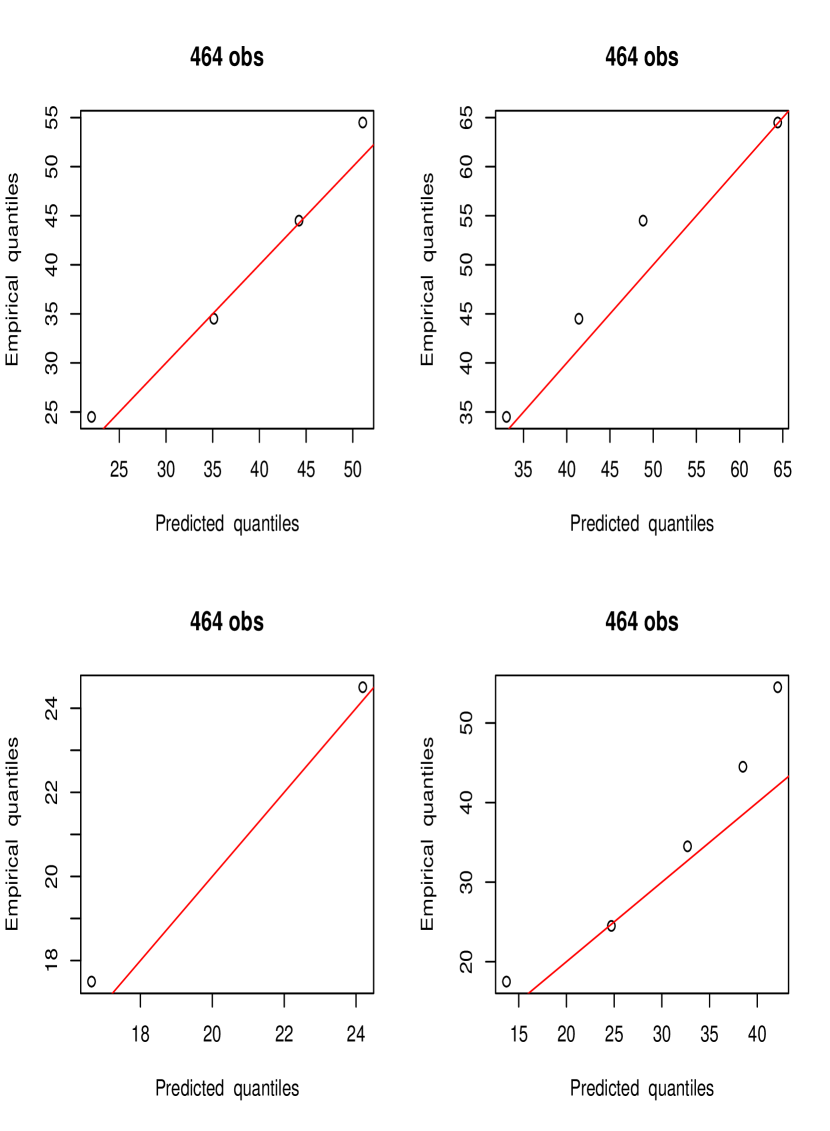
Figure 2: Questionnaire data. Q–Q plots of empirical versus predicted quantiles for untransformed Omnireg solution for four data subsets obtained by partitioning the location $\hat{f}(\mathbf{x})$ and $\hat{s}(\mathbf{x})$ estimates at their respective medians.

Figure 2 shows four Q–Q plots of the empirical versus predicted quantiles of the marginal distribution of age (Section 4.1) based on the untransformed solution. Each plot represents data within a joint interval of $\hat{f}(\mathbf{x}_{i})$ and $\hat{s}(\mathbf{x}_{i})$ values. The interval boundaries for $\hat{f}(\mathbf{x}_{i})$ are obtained by partitioning at its corresponding median (rows – bottom to top). Within each such location interval separate intervals for $\hat{s}(\mathbf{x}_{i})$ are constructed using its median evaluated within that location interval (columns – left to right). Thus the lower left plot is based on the  25% of the observations with the smallest locations and smallest scales. The top right involves the 25% of the observations with jointly the largest estimated locations and scales. Because of the censoring this marginal distribution is observable only at the six values that separate the censoring intervals. In Fig. 2, points representing extreme empirical  quantiles based on less than $20$ observations are not shown due to their instability. One sees In Fig. 2 that the predicted quantiles approximately follow the actual empirical quantiles. However there are a few clear discrepancies in the right plots representing the larger scale estimates.

Figure 3 shows the sequence of transformation solutions for seven iterations of the optimal transformation procedure described in Section 3. The respective transformations are defined only at the six values separating the censoring intervals. To aid interpretation lines connecting the corresponding points representing the same solution are included. Here blue represents the result of the first iteration, red the last, and black the intermediate ones. After about four iterations convergence appears to be achieved. The result at the seventh iteration (red) is chosen as the optimal transformation estimate $\hat{g}(y)$.

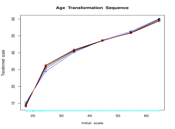
Figure 3: Solutions at successive iterations of the optimal transformation algorithm on questionnaire data. First is colored blue, two through six black and seventh red.

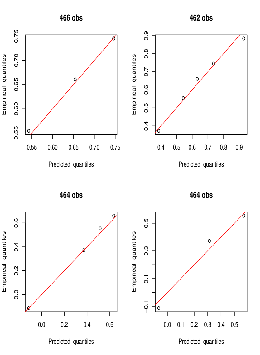
Figure 4: Questionnaire data. Q–Q plots of empirical versus predicted quantiles for transformed $\hat{g}(y)$ OmniReg solution for four data subsets obtained by partitioning the corresponding location $\hat{f}(\mathbf{x})$ and $\hat{s}(\mathbf{x})$ estimates at their respective medians.

Figure 4 shows Q–Q plots of the empirical distribution of transformed age $\hat{g}(y)$ versus that predicted by its corresponding location $\hat{f}(\mathbf{x})$ and scale $\hat{s}(\mathbf{x})$ functions. The four data subsets are constructed in the same manner as in Fig. 2. Here in the transformed setting one sees a closer correspondence with model predictions especially for the larger scale values.

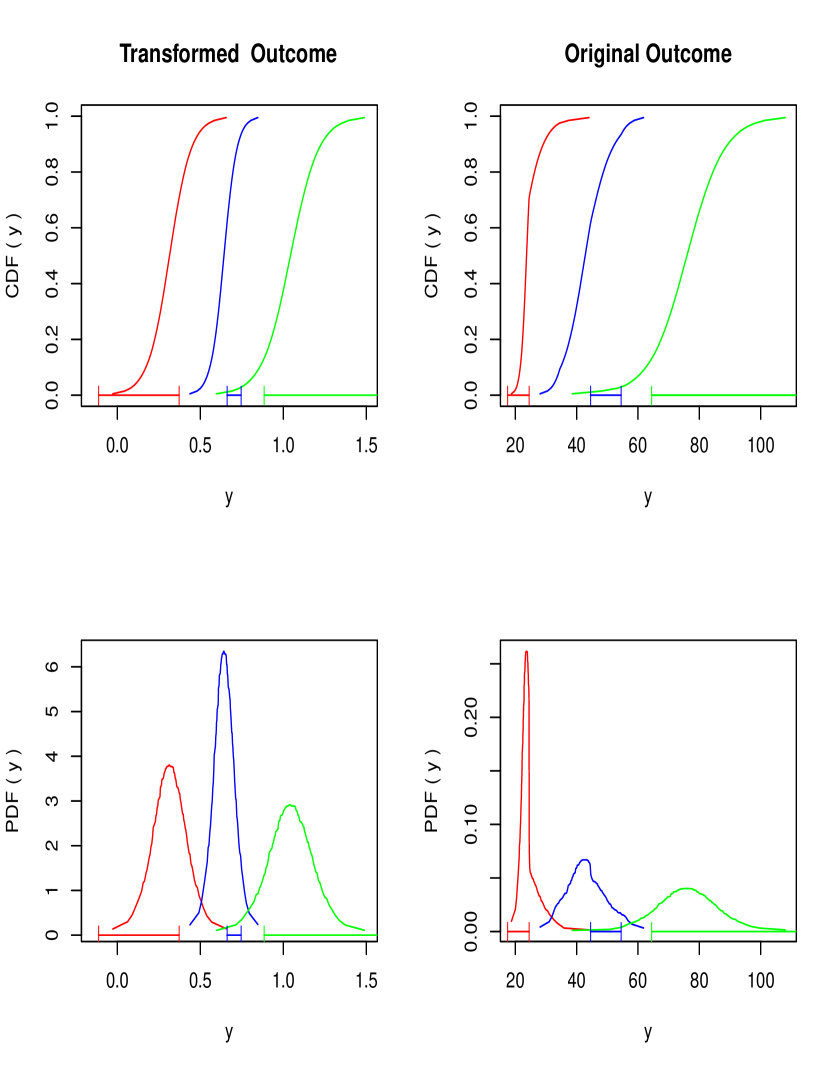
Figure 5: Predicted probability distributions for three questionnaire data test set observations. Left: transformed setting. Right: original untansformed (age) setting. Upper: CDF, $\hat{F}(y\,|\,\mathbf{x})$. Lower: PDF, $\hat{p}(y\,|\,\mathbf{x})$. Bottom intervals represent those specified for the corresponding three censored observations.

Unlike usual regression procedures that return a single number as a prediction, OmniReg produces a function representing the predicted distribution of $y$ given $\mathbf{x}$. Figure 5 shows such predicted functions for $\mathbf{x}$-values of three observations in the validation data set. The left plots show the distributions in the transformed setting, whereas the right plots reference the original outcome variable (age). The upper plots show the cumulative distributions and the lower ones show the corresponding probability density functions. The intervals indicated at the bottom of each plot represent the actual censoring intervals for the three chosen observations (Table 3). Perhaps the most useful representation is the predicted CDF of the original untransformed $y$ (upper right), since from it one can directly read probability intervals for $y$ (age) predictions.

6.2 Online news popularity data

This data set (Fernandes, Vinagre and P. Cortez 2015) is available for download from the Irvine Machine Learning Data Repository. It summarizes a heterogeneous set of features about articles published by Mashable web site over a period of two years. The goal is to predict the number of shares in social networks (popularity). There are $N=39797$ observations (articles). Associated with each are $p=59$ attributes to be used as predictor variables $\mathbf{x}$. These are described at the download web site https://archive.ics.uci.edu/ml/datasets/online+news+popularity#. The outcome variable for each article is its number of shares. For this analysis these data are randomly divided into $30000$ observations for model construction, $5000$ for selecting the number of trees in each model  (7) (8) , and $4797$ observations for validation.

Figure 6: Distribution of $\log_{10}(shares)$ for the online news data.

The number of shares in these data varies from less than 100 to over 100000 and is heavily skewed toward larger values. For data of this type it is common to apply a log–transform to the outcome variable. Figure 6 shows a histogram of $y=$ $\log_{10}(shares)$ for these data. There seems to be a sharp change in the nature of this distribution at $1000$ shares. In the first analysis we directly model $y=$ $\log_{10}(shares)$ without performing any further transformation (Section 2). In the second we apply the technique of Section 3 to estimate the optimal transformation $\hat{g}(\log_{10}(shares))$.

Since these data are uncensored one can directly analyze the predicted residuals as described in Section 4.2. Fig. 7 shows nine standardized residual Q–Q plots based on the untransformed model using nine different subsets of the validation data set. These subsets were constructed as described in Section 6.1 (Fig. 2), but with partitions at the corresponding 33% quantiles of $\hat{f}(\mathbf{x}_{i})$ and $\hat{s}(\mathbf{x}_{i})$ to create nine regions.

Each frame in Fig. 7  displays four Q-Q plots. The black lines represent a comparison of the estimated standardized residuals to a logistic distribution. For reference, the orange, green and violet lines show comparisons to the normal, Laplace and slash distributions respectively. The slash (Rogers and Tukey 1972) is the distribution of the ratio of normal and uniform random variables and has very heavy tails. The blue line in each plot is the 45–degree diagonal. Here one sees that the standardized residuals predicted by the model do not closely follow a logistic distribution (black line) for any of the location–scale defined data subsets. This suggests that inference based on this model using the log–transformation is highly suspect.

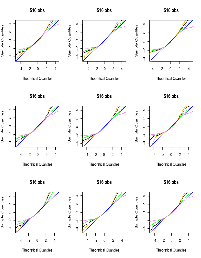
Figure 7: Online news popularity data. Diagnostic Q-Q plots of actual vs. predicted distribution of untransformed standardized residuals $(y\,\,-$ $\hat{f}(\mathbf{x}))/\hat{s}(\mathbf{x})$ for nine data subsets delineated by joint intervals of the $1/3$ quantiles of estimated location $\hat{f}(\mathbf{x})$ and scale $\hat{s}(\mathbf{x})$. The black, orange, green and violet lines respectively represent comparisons to logistic, normal, Laplace and slash distributions.

Applying the optimal transformation procedure of Section 3 to the log-transformed data one obtains the sequence of transformation estimates for each iteration shown in Fig. 8. The first estimate is colored blue, the seventh red, and the intermediates black. The blue hash marks below the abscissa delineate 1% intervals  of the $y$-distribution. Convergence appears to occur after three iterations.

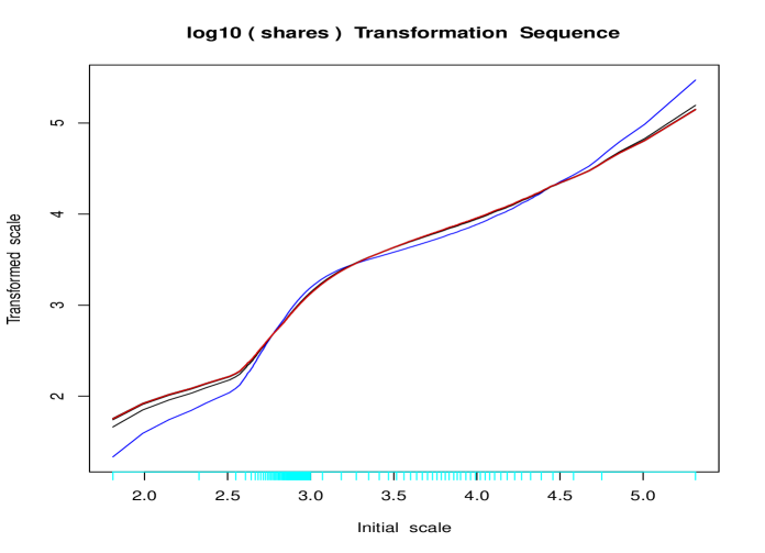
Figure 8: Solutions at successive iterations of the optimal transformation algorithm on online news popularity data. First is colored blue, two through six black and seventh red. The blue hash marks below the abscissa delineate 1% intervals  of the $y$-distribution.

Using the model $\hat{g}(\log_{10}(shares))$ based on the seventh (red) transformation produces the corresponding standardized residual plots shown in  Fig. 9. Here the predicted residuals very closely follow a standard logistic distribution (black line) for all data subsets. A slight exception might be the lower right plot (small location, large scale) where the extreme positive residuals appear somewhat too large. This diagnostic provides little evidence of overall lack of fit of the transformed model or violation of its assumptions. Of course, one cannot absolutely exclude the possibility that there are other diagnostics that might demonstrate such evidence.

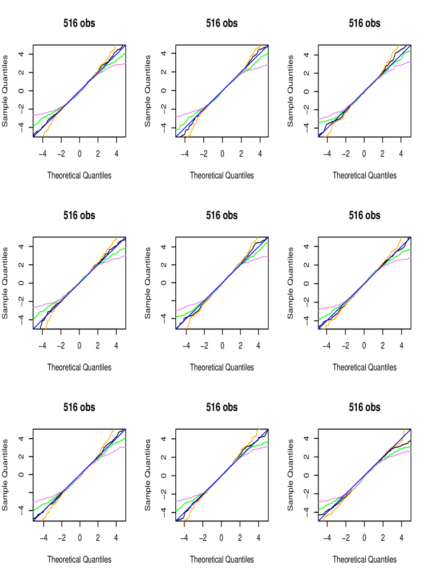
Figure 9: Online news popularity data. Diagnostic Q-Q plots of actual vs. predicted distribution of optimal transformed standardized residuals $(\hat{g}(y)\,-$ $\hat{f}(\mathbf{x}))/\hat{s}(\mathbf{x})$ for nine data subsets delineated by joint intervals of the $1/3$ quantiles of estimated location $\hat{f}(\mathbf{x})$ and scale $\hat{s}(\mathbf{x})$. The black, orange, green and violet lines respectively represent comparisons to logistic, normal, Laplace and slash distributions.

Figure 10 shows curves representing the model predicted probability distributions of $\log_{10}(shares)$ for $\mathbf{x}$-values of three observations taken from the validation data set. The format is the same as in Fig. 5. The circles at the bottom of each plot represent the actual realized $\log_{10}(shares)$ for these three chosen observations. Distribution asymmetry and heteroscedasticity are evident in the untransformed setting (right frames). Prediction probability intervals can be directly determined from the upper right plot.

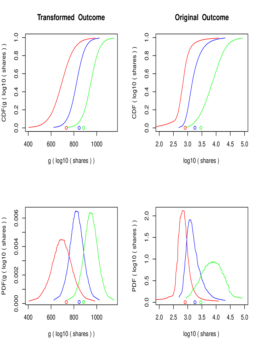
Figure 10: Predicted probability distributions for three test set observations from the online news popularity data. Left: transformed setting. Right: original untansformed (log–shares) setting. Upper: CDF, $\hat{F}(y\,|\,\mathbf{x})$. Lower: PDF, $\hat{p}(y\,|\,\mathbf{x})$. Bottom points represent the corresponding recorded $\log_{10}(shares)$ for the three selected observations.

6.3 Million Song Data Set

These data are a subset of the Million Song Data Set and are also available for download from the Irvine Machine Learning Data Repository. It consists of a training data set of 463715 and a test set of 51630 song recordings. We divide a randomly selected subsample of the training data into a learning data subset of 50000 observations and one for model selection consisting of  20000 observations. All diagnostics are performed on the 51630 song test data set. There are 89 predictor variables measuring various acoustic properties of the recordings. The outcome variable is the year the recording was made ranging from 1922 to 2011.

Figure 11: Distribution of recording year for the million song data set.

Figure 11 shows a histogram of the outcome variable $y$. There are relatively few songs in the data set recorded before 1955. Modeling the data without transformations (Section 2) produces the standardized residual diagnostic plots on the test data set shown in Fig. 12. The data subsets are constructed in the same manner as for Fig. 7. Again, none of the predicted standardized residual distributions in any of the data subsets are remotely close to being standard logistic (black line).

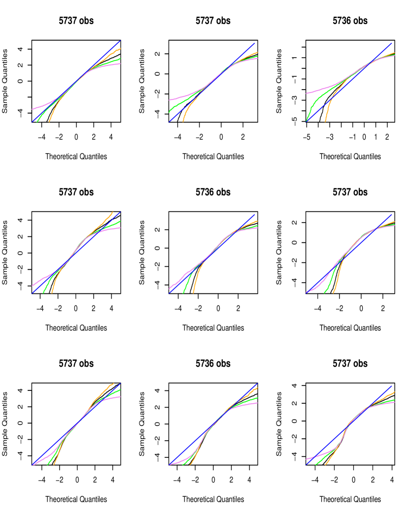
Figure 12: Million song data set. Diagnostic Q-Q plots of actual vs. predicted distribution of untransformed standardized residuals $(y\,-$ $\hat{f}(\mathbf{x}))/\hat{s}(\mathbf{x})$ for nine data subsets delineated by joint intervals of the $1/3$ quantiles of estimated location $\hat{f}(\mathbf{x})$ and scale $\hat{s}(\mathbf{x})$. The black, orange, green and violet lines respectively represent comparisons to logistic, normal, Laplace and slash distributions.

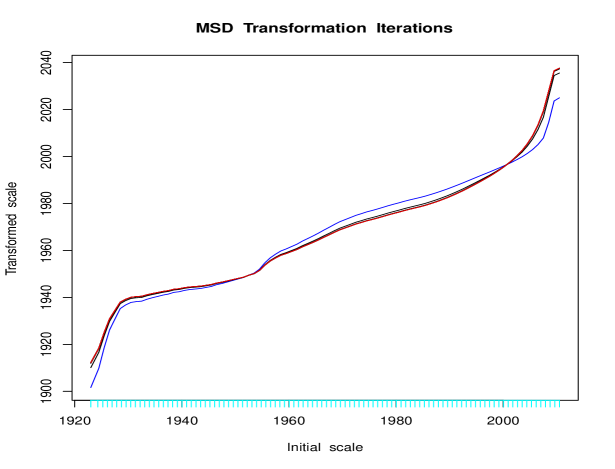
Figure 13: Solutions at successive iterations of the optimal transformation algorithm on million song data set. First is colored blue, two through six black and seventh red.

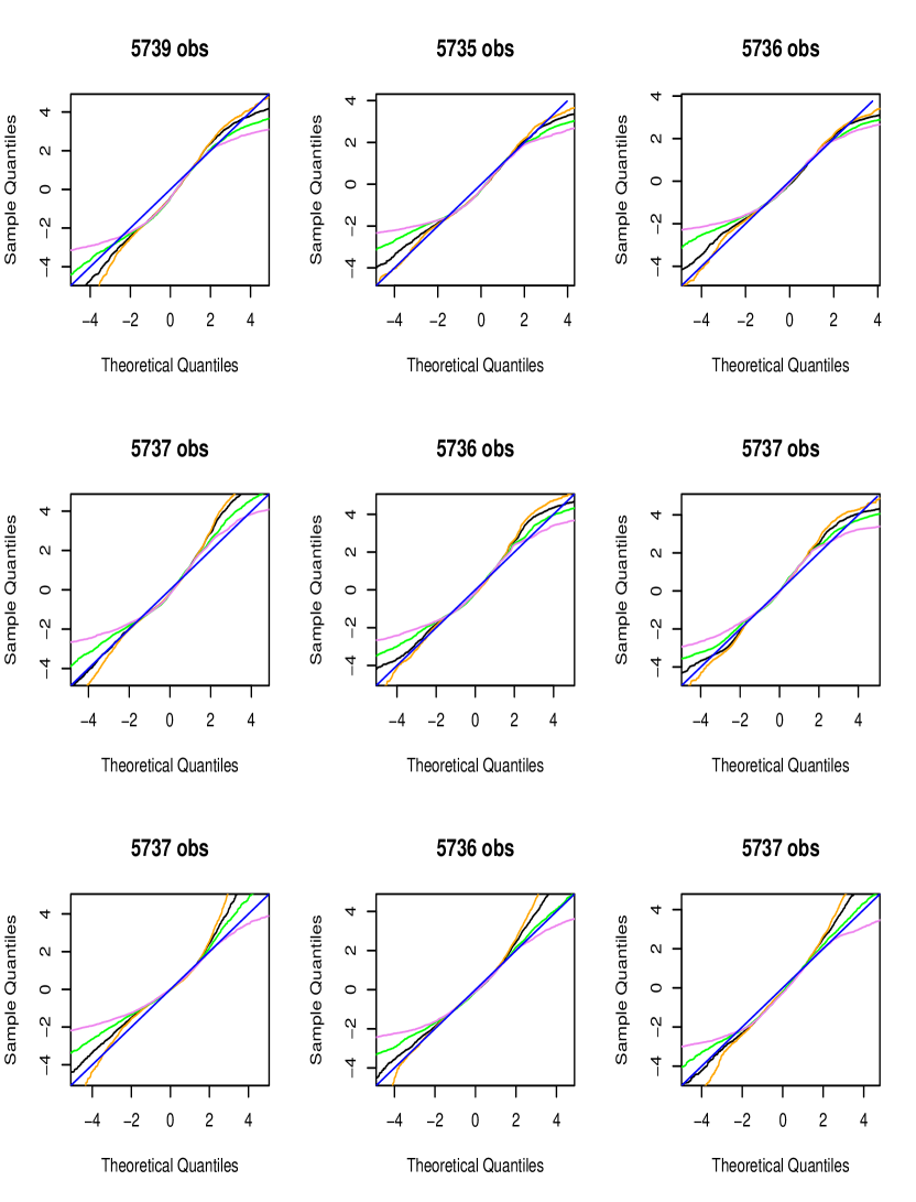
Figure 14: Million song data set. Diagnostic Q-Q plots of actual vs. predicted distribution of transformed standardized residuals $(\hat{g}(y)\,\,-$ $\hat{f}(\mathbf{x}))/\hat{s}(\mathbf{x})$ for nine data subsets delineated by joint intervals of the $1/3$ quantiles of estimated location $\hat{f}(\mathbf{x})$ and scale $\hat{s}(\mathbf{x})$. The black, orange, green and violet lines respectively represent comparisons to logistic, normal, Laplace and slash distributions.

Applying the optimal transformation strategy of Section 3 produces the sequence of transformation estimates for seven iterations shown in Fig. 13. There is little change after two iterations. Figure 14 shows the corresponding standardized residual Q–Q plots for the seventh transformed solution. Although not perfect, these residuals much more closely follow a logistic distribution (black line) than for the untransformed solution (Fig. 12). The residual distributions for some of the samples are seen to differ mainly for extreme positive values where the data have somewhat narrower tails.

Figure 14 suggests that the optimal transformation strategy of Section 3 based on the additive symmetric error model (13) has not produced totally accurate probability estimates. This in turn suggests trying the asymmetric procedure of Section 5. Figure 15 shows the resulting diagnostic Q–Q plots when the second asymmetric algorithm of Section 5 is applied to the original untransformed outcome data.  The result is seen to be (at best) no better than the corresponding symmetric error results (Fig. 12).

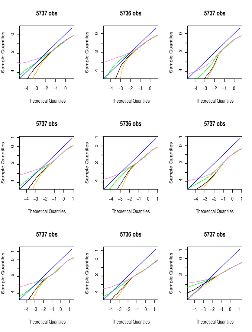
Figure 15: Million song data set. Diagnostic Q-Q plots of actual vs. predicted distribution of untransformed asymmetric standardized residuals (22) for nine data subsets delineated by joint intervals of the $1/3$ quantiles of estimated location $\hat{f}(\mathbf{x})$ and those of the geometric mean $\sqrt{\hat{s}_{l}(\mathbf{x})\hat{s}_{u}(\mathbf{x})}$ of the scales. The black, orange, green and violet lines respectively represent comparisons to logistic, normal, Laplace and slash distributions.

Figure 16 shows the sequence of transformations produced by the optimal transformation strategy of Section 3 used in conjunction with the asymmetric estimation procedure of Section 5. The estimated optimal transformation (red) has the same general shape as the one produced by the symmetric procedure (Fig. 13) with small to moderate differences mainly at the lower extreme.

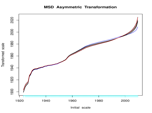
Figure 16: Solutions at successive iterations of the asymmetric optimal transformation algorithm on million song data set. First is colored blue, two through six black and seventh red.

Figure 17 shows the resulting diagnostic plots produced by the asymmetric error model in its optimally transformed setting. For this diagnostic the respective data subsets represent the validation data partitioned at the 33% quantiles of their location (mode) estimates $\hat{f}(\mathbf{x})$ (bottom to top) and the 33% quantiles of the geometric mean of their two scale estimates $\sqrt{\hat{s}_{l}(\mathbf{x})\,\hat{s}_{u}(\mathbf{x})}$ (left to right). The (asymmetric) standardized residuals (22) are seen to very closely follow a standard logistic distribution (3) for all data subsets.

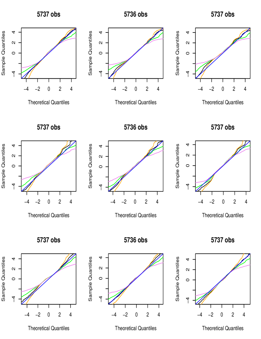
Figure 17: Million song data set. Diagnostic Q-Q plots of actual vs. predicted distribution of transformed asymmetric standardized residuals (22) for nine data subsets delineated by joint intervals of the $1/3$ quantiles of estimated location $\hat{f}(\mathbf{x})$ and geometric mean $\sqrt{\hat{s}_{l}(\mathbf{x})\hat{s}_{u}(\mathbf{x})}$ of the scales estimates. The black, orange, green and violet lines respectively represent comparisons to logistic, normal, Laplace and slash distributions.

Figure 18 shows plots of the lower $\hat{s}_{l}(\mathbf{x})$ (blue) and upper $\hat{s}_{u}(\mathbf{x})$ (red) scale estimates against corresponding location estimates $\hat{f}(\mathbf{x})$ in the optimal transformed setting. Here the upper scales are seen to be almost constant (homoscedastic) whereas the lower scales vary by roughly a factor of four. Neither seem to have any association with the location estimates.

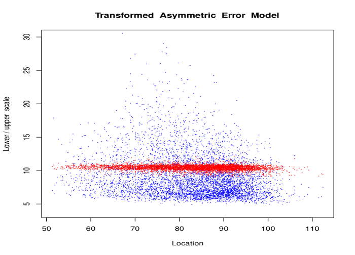
Figure 18: Million song data. Upper scale estimates $\hat{s}_{u}(\mathbf{x})$ (red) and lower scale estimates $\hat{s}_{l}(\mathbf{x})$ (blue) vs. mode $\hat{f}(\mathbf{x})$ for asymmetric optimal transformed setting.

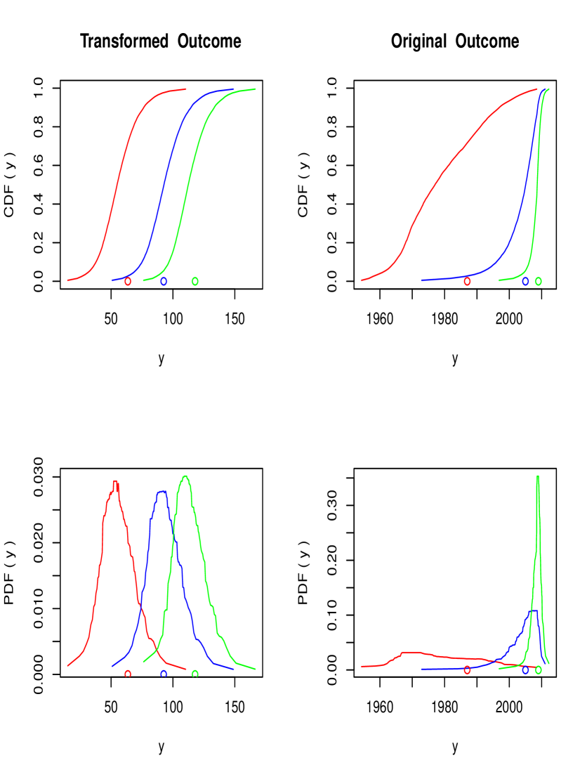
Figure 19: Predicted probability distributions based on the optimally transformed asymmetric model for three test set observations from the million song data. Left: transformed setting. Right: original untansformed (year) setting. Upper: CDF, $\hat{F}(y\,|\,\mathbf{x})$. Lower: PDF, $\hat{p}(y\,|\,\mathbf{x})$. Bottom points represent the corresponding dates for the three selected recordings.

Figure 19 shows the predicted recording year probability distributions for three recordings in the test data set based on the transformed asymmetric model. The format is the same as that in Figs. 5 and 10. Unlike the distributions in those figures that are based on symmetric transformed models, here one sees some asymmetry of the distributions in the transformed setting. In the original outcome setting (recording year) there is seen to be massive skewness and heteroscedasticity. The predictive model is pretty certain that the recording indicated by green was made after 2005. For the blue recording it predicts somewhere between 1990 and 2010. It reports having little indication as to when the recording in red was made except that it is likely, but not certainly, before the other two. The circles at the bottom of each plot represent the actual dates for these three recordings.

7 Ordinal regression

In the examples of Section 6 there is a known measurement scale for the values of the outcome variable $y$. Values of $y$ as well as the interval bounds $\{a_{i},b_{i}\}_{1}^{N}$ in (5) (6) reference this scale. In ordinal regression no such measurement scale exists. Only a relative order relation among the $y$-values is specified. Usually ordinal regression is applied in the context of many ties so that there are only a few $K$ unique grouped values such as $y\in\{$small, medium, large, extra large$\}$. For any set of joint predictor variable values $\mathbf{x}$ the main goal is to predict $p(y\in k\,|\,\mathbf{x})$ where $k=1\cdot\cdot\cdot K$ labels the groups. In this sense ordinal regression can be viewed as classification where there is an order relation among the class labels.

OmniReg with optimal transformations (Sections 2 , 3 and 5) is fundamentally a (generalized) ordinal regression procedure. Its solutions depend only on the values of the cumulative distribution (ranks) of $y$, $\hat{F}(y)$ (16). As noted in Section 2.1 tied $y$-values can be considered as interval censored with lower bound at the midpoint of its value and the next lower value, and upper bound the midpoint of its value and the next higher value. The lower bound of the first group can be taken to be $-\infty$ and the upper bound of the last $\infty$. This was the strategy used in Section 6.1 (Table 3).

Note that for the problem analyzed in Section 6.1 there was no fundamental requirement that the censoring intervals be on the age measurement scale. Any scale that produces the same order (grouping) could have been used. Changing the measurement scale is equivalent to changing the starting transformation for the iterative procedure of Section 3. Except for possible numerical effects the resulting solutions should be essentially equivalent.

Censoring in ordinal regression is easily incorporated with this approach. If it is unknown which of several adjacent groups contains training observation $y_{i}$, its lower bound $a_{i}$ is set to the minimum of the lower bounds over those groups, and its upper bound $b_{i}$ is set to the maximum of the corresponding group upper bounds. Also, with this approach to ordinal regression computation does not depend on the number of groups.

The predicted probability of an observation being in the $k$th group is given by $\hat{p}(y\in k\,|\,\mathbf{x})=CDF(\hat{g}(b_{k}))-CDF(\hat{g}(a_{k}))$ where $a_{k}$ and $b_{k}$ are respectively the lower and upper bound specified for the $k$th group on the chosen initial measurement scale. $CDF(z)$ is given by (18) for symmetric models, and (21) for asymmetric models, based on the OmniReg function estimates $\hat{g}(y)$, $\hat{f}(\mathbf{x})$, and $\hat{s}(\mathbf{x})$ or $\hat{s}_{l}(\mathbf{x})$, $\hat{s}_{u}(\mathbf{x})$.

8 Related work

The OmniReg procedure presented here combines approaches from several separate topics each of which has a long and rich history in Statistics, Econometrics and Machine Learning. The procedure presented in Section 2 is a straight forward generalization of Tobit analysis (Tobin 1958) to incorporate logistic errors, general censoring, heteroscedasticity, and general nonparametric function estimation via boosted tree ensembles. There are many previous works that incorporate various subsets of these generalizations.

8.1 Censoring

Although various forms of censoring actually occur in many types of applied regression problems, it has been studied mainly in the context of survival analysis where the outcome variable $y$ is time to some event. Right censoring occurs when that time exceeds the end of the study. The most popular tool for survival analysis is the Cox proportional hazards model (Cox 1972) which estimates the hazard function $\lambda(y)$ up to a multiplicative function of time

$$\lambda(y\,|\,\mathbf{x})=p(y\,|\,\mathbf{x})/(1-CDF(y\,|\,\mathbf{x}))=h(y)\cdot\exp(f(\mathbf{x}))\text{.}$$

Here $h(y)$ is an unknown baseline hazard and the function $f(\mathbf{x})$ is estimated from the data. Cox originally proposed a linear model $f(\mathbf{x})=\mathbf{\beta}^{t}\mathbf{x}$, but various authors have since presented nonlinear generalizations. OmniReg (Sections 2 and 3) can be applied to survival data with mixtures of any type of censoring. Because it estimates $p(y\,|\,\mathbf{x})$ it can be used to directly estimate the absolute hazard $\lambda(y\,|\,\mathbf{x})$.

8.2 Transformations

Transforming an outcome variable $y$ in order to increase its compatibility with regression procedure assumptions has a long history in Statistics. Mosteller and Tukey (1977) proposed a ladder of reexpressions for different variable types based upon their realizable values. Box and Cox (1964) proposed the first data driven approach by selecting a power transformation $g_{\alpha}(y)=y^{\alpha}$ for numeric variables that maximizes the data Gaussian likelihood in the context of homoscedasticity and linear models.

Gifi (1990), and Breiman and Friedman (1985), proposed estimating outcome transformations for additive modeling by minimizing

$$\sum_{i=1}^{N}\left.\left(g(y_{i})-\sum_{j=1}^{p}h_{j}(x_{ij})\right)^{2}\right/\sum_{i=1}^{N}g^{2}(y_{i})$$ (23)

jointly with respect to centered functions $g(y)$ and $\{h_{j}(x_{j})\}_{1}^{p}$ under a smoothness constraint. With Gifi (1990) smoothness was imposed by restricting all functions to be in the class of monotone splines with a given number and placement of knots. Solving (23) then becomes a canonical correlation problem implemented by alternating linear least–squares parameter estimation. Breiman and Friedman (1985) directly used nonparametric data smoothers to estimate all functions also using an alternating approach similar to that used in Section 3.  Both approaches assume an additive homoscedastic model for $g(y)$ as a function of $\mathbf{x}$.

Solutions to (23) maximize the correlation between $g(y)$ and $\sum_{j=1}^{p}h_{j}(x_{j})$ over the joint distribution $p(\mathbf{x},y)$ of $y$ and $\mathbf{x}$. As a result the solution transformations depend on the marginal distribution $p(\mathbf{x})$ of the predictor variables $\mathbf{x}$ (Buja 1990). A consequence is that the expected solutions of (23) applied to data arising from the regression model

$$g^{\ast}(y_{i})=\sum_{j=1}^{p}h_{j}^{\ast}(x_{ij})+\varepsilon_{i}$$

with $\varepsilon_{i}\sim N(0,\sigma^{2})$ will not generally be $g(y)=$ $g^{\ast}(y)$ and $\{h_{j}(x_{j})=h_{j}^{\ast}(x_{j})\}_{1}^{p}$. Distributions of $\mathbf{x}$ that tend to exhibit clustering are especially problematic.

In order to alleviate this problem Tibshirani (1988) proposed finding transformations $g(y)$ and $\{h_{j}(x_{j}\}_{1}^{p}$ that that minimize

$$\sum_{i=1}^{N}\left(g(y_{i})-\sum_{j=1}^{p}h_{j}(x_{j})\right)^{2}$$

where the monotone function $g(y)$ is taken to be the variance stabilizing transformation

$$Var\left(\left.g(y)\,\right|\sum_{j=1}^{p}h_{j}(x_{j})\right)=\text{ \emph{constant}.}$$ (24)

Solutions are obtained by an alternating optimization algorithm.

In the language of this paper (24) will hold if the location function $f(\mathbf{x})$ (13) is additive in $\mathbf{x}$ and the scale function $s(\mathbf{x})$ is independent of $f(\mathbf{x})$. In particular, (24) does not necessarily imply homoscedasticity $s(\mathbf{x})=\,$constant in the transformed setting $g(y)$. For all the examples in this paper the association between the location and scale estimates for the optimal $\hat{g}(y)$ happened to be quite weak but there was still considerable variation in scale, as with for example $\hat{s}_{l}(\mathbf{x})$ in Fig. 18.

The transformation strategy outlined in Sections 2, 3 and 5 is directly regression based in that it is conditional on $\mathbf{x}$. The basic assumption is that the standardized residuals (19) (22) follow a standard logistic distribution (3) at any $\mathbf{x}$ irrespective of the distribution of $\mathbf{x}$. Also note that the estimate $\hat{g}(y)$ obtained from (16) is automatically monotonic.

8.3 Quantile regression

For known $y$-values and in the absence of censoring a natural alternative to the procedures described in Sections 2, 3 and 5 is quantile regression based on gradient boosted trees. One can estimate the $p$th quantile function, $q_{p}(\mathbf{x)}$, of $p(y\,|\,\mathbf{x})$ using the loss function

$$L(y,q_{p})=(y-q_{p})\,[p\,I(y\geq q_{p})+(p-1)\,I(y<q_{p})]\text{.}$$ (25)

Friedman (2001) suggested using (25) in the context of gradient boosting and it has been incorporated in many implementations (see Ridgeway 2007 and Pedregosa 2011). Recently, Athey, Tibshirani, and Wagner (2017) implemented quantile regression in random forests. With boosted tree quantile regression (25) simply replaces (5) as the loss function in the procedure outlined in Sections 2.2 and 2.3, and only one function is estimated separately for each quantile $p$. One can use this procedure to independently estimate functions $q_{p}(\mathbf{x)}$ for several quantiles $\{p_{k}\}_{1}^{P}$, and then  for any $\mathbf{x}$ use $\{q_{p}(\mathbf{x)\}}_{1}^{P}$ to approximate the corresponding quantiles of $p(y\,|\,\mathbf{x})$. This approach makes no assumptions concerning a generating model for $p(y\,|\,\mathbf{x})$, such as (13) or (20). It thus may provide useful results in applications where those assumptions are seriously violated. However, when they are not decreased accuracy can result.

8.4 Direct maximum likelihood estimation

For $y$-values on a known measurement scale, another natural alternative to the procedure described in Sections 2, 3 and 5 is applying direct maximum likelihood such as in GAMLSS (Rigby and Stasinopoulos 2006). A parameterized probability density for $p(y\,|\,\mathbf{x})$ is hypothesized and then its parameters are fitted as functions of the predictor variables $\mathbf{x}$ by maximum likelihood. Parametric, linear and additive functions are considered. These are fit to data by numerically maximizing the corresponding (non convex) log–likelihood with respect to the parameters defining all of the functions of $\mathbf{x}$. The assumed probability density can have parameters controlling its location, scale, skewness and kurtosis which are all modeled as functions of the predictors in this manner.

A similar paradigm is used in Sections 2 and 5 based on the two and three parameter logistic distributions. A difference is that the parameters are taken to be more flexible functions of $\mathbf{x}$ as represented by boosted decision tree ensembles. It is straightforward to generalize the gradient tree boosting strategy of Section 2 and 5 to other distributions with more that two or three parameters as functions of the predictor variables $\mathbf{x}$. Whether such added complexity translates to improved or reduced accuracy will be application dependent. In any application the diagnostics described in Sections 4.1 and 4.2  may be helpful in assessing model deficiencies.

The central difference between the GAMLSS method and OmniReg lies in the optimal transformation strategy (Section 3). The GAMLSS approach assumes that the hypothesized parametric distribution describes $p(y\,|\,\mathbf{x})$. OmniReg assumes that there exists some transformation $g(y)$ for which $p(g(y)\,|\,\mathbf{x})$ follows the specified distribution. It then nonparametrically estimates that transformation $g(y)$ jointly with its corresponding distribution parameters as functions of $\mathbf{x}$. This substantially enlarges the scope of application. The data examples of Sections 6.2 and 6.3 illustrate the gains that  can be made by this transformation strategy. They also illustrate that the optimal transformations for a given problem need not be close to any function in commonly assumed parametric families such as the power family $g_{\alpha}(y)=y^{\alpha}$.

Arrays of multiple Q–Q plots each based on different regions of the $\mathbf{x}$-space were proposed by van Buuren and Fredriks (2001). The diagnostic plots of Section 4.2 are a straightforward generalization. Those of Section 4.1 can be viewed as a generalized version for arbitrarily censored data.

8.5 Ordinal regression

There is a large literature on ordinal regression (see McCCullagh 1980 and Gutiérrez et. al. 2016). A common method is to apply a sequence of binary linear logistic regressions to separately estimate the probability of being below each of the successive group boundaries. The probability of being within each of the groups is then obtained by successive differences between these estimates. In order to avoid negative values the coefficients of all linear models are constrained to be the same, with only the intercepts changing.

The approach most similar in spirit to the one here is Messner et. al. (2014). They propose a statistical model similar to (3) (13). The location $f(\mathbf{x})$ and log-scale functions $\log(s(\mathbf{x}))$ are modeled as linear functions of the predictor variables $\mathbf{x}$ by numerical maximum likelihood. The transformation $g(y)$ is preselected and not systematically fit to the data.

9 Point prediction

The focus of this work is on the estimation of the distribution functions $p(y\,|\,\mathbf{x})$. These can be used to infer likely values of $y$ for given $\mathbf{x}$-vectors. Sometimes the goal of regression is to return a single value that minimizes the prediction risk at $\mathbf{x}$

$$h(\mathbf{x})=\arg\min_{h}\int L(y,h)\,p(y\,|\,\mathbf{x})\,dy\text{.}$$ (26)

Here $L(y,h)$ represents a loss, relevant to the application at hand, for predicting $h$ when the actual value is $y$. One way to attempt to solve (26) is

$$\hat{h}(\mathbf{x})=\arg\min_{h(\mathbf{x})\in H}\sum_{i=1}^{N}L(y_{i},h(\mathbf{x}_{i}))\text{.}$$ (27)

Here $H$ is a class of functions usually defined by the fitting procedure employed. An alternative strategy is to use

$$\hat{h}(\mathbf{x})=\arg\min_{h}\int L(y,h)\,\hat{p}(y\,|\,\mathbf{x})\,dy$$ (28)

where $\hat{p}(y\,|\,\mathbf{x})$ is an estimate of $p(y\,|\,\mathbf{x})$, for example through (4) (5) (6). For some $L(y,h)$ and $\hat{p}(y\,|\,\mathbf{x})$, (28) can be solved analytically. Otherwise it can be easily solved by numerical methods. Note that there is no requirement that $L(y,h)$ be convex in (28). Usually (27) is used when there is no censoring, and (28) is applied when censoring is present. Which of the two is best in terms of accuracy in any particular application depends on the specific nature of that application. If there exists a validation data set $V$ not used for training with known (uncensored) $y$-values one can use

$$CV=\sum_{i\in V}L(y_{i},\hat{h}(\mathbf{x}_{i}))$$ (29)

to estimate the accuracy of any $\hat{h}(\mathbf{x})$. An advantage of (28) is that solutions for a variety of loss functions $L(y,h)$, as well as other statistics, can be easily obtained without having to recompute $\,\hat{p}(y\,|\,\mathbf{x})$.

10 Discussion

The goal of this work (OmniReg) is to provide a general unified procedure that can be used for predictive inference in a variety of regression problems. These include heteroscedasticity, asymmetry, ordinal regression, and general censoring.

Censoring has received relatively little attention in machine learning even though it is a common occurrence in regression problems. Often there are restrictions on the measured values of the outcome $y$. Section 6.1 illustrates a case where measurements of a continuous outcome (age) are restricted to six discrete values (intervals). Another common restriction is where the observed $y$-values cannot be negative, such as payout on insurance policy claims. There is usually a large mass of zero–valued outcomes along with some positive ones. In this case it is not straight forward to formulate and estimate a corresponding $p(y\,|\,\mathbf{x})$. One way (Tobin 1958) is to consider the observed $y$-values as censored below zero measurements of a latent variable $y^{\ast}$ with an unrestricted $p(y^{\ast}\,|\,\mathbf{x})$. This can then be estimated from the data using the techniques of Sections 2, 3 and 5.

Formal predictive inference has also received relatively little attention. However, informal inference is at the heart of prediction. The presumption is that a predicted value $\hat{f}(\mathbf{x})$ is “somewhere close” to the actual outcome $y$-value. Predictive inference simply quantifies this concept through an estimated probability distribution. As seen in the data examples of Section 6 the nature of “somewhere close” can be very different for different predictions in the same problem. Also this probability distribution can be used to obtain point estimates for any loss function through (28). These can sometimes be more accurate than corresponding direct estimates (27).

A central feature of OmniReg is the optimal transformation strategy of Section 3. This extends the applicability of the method to a much wider class of problems. It is also at the heart of the ordinal regression strategy of Section 7. As seen in the data examples, a particular assumed probability distribution $p(y\,|\,\mathbf{x})$ (here (4) or (20)) is seldom appropriate for the original outcome $y$. However, there is often a corresponding optimal transformation $g(y)$ for which it is much more appropriate. This optimal transformation may not be close to any member of a common parametric family as was seen in Figs. 8, 13 and 16.

The basic OmniReg method is indifferent to the technique used to obtain the parameter function estimates $\hat{f}(\mathbf{x})$, $\hat{s}(\mathbf{x})$, or $\hat{s}_{l}(\mathbf{x})$, $\hat{s}_{u}(\mathbf{x})$. An iterative strategy based on gradient boosted trees was used in Sections 2.3, 3 and 5. This seems to work well in a variety of applications. However, there may be some for which other methods work as well or better. A crucial but delicate ingredient is regularization, especially for the location estimate. An overfitted location estimate $\hat{f}(\mathbf{x})$ will cause a severe negative bias in the log–scale estimates $\log(\hat{s}(\mathbf{x})),$ or $\log(\hat{s}_{l}(\mathbf{x}))$, $\log(\hat{s}(\mathbf{x}))$. This produces inaccurate (over optimistic) estimates of the corresponding scale functions, which would be detected by the diagnostics of Section 4. Early stopping based on cross–validation seems to work well for the estimation method used here. Other methods may require different regularization strategies.

Employing a different function estimation method changes the function class $F$ in (6) or its asymmetric counterpart (Section 5). This criterion is minimized with respect to the transformation function $g(y)$ jointly with the parameter functions $f(\mathbf{x})$, $s(\mathbf{x})$, or $s_{l}(\mathbf{x})$, $s_{u}(\mathbf{x})$ all in $F$. Thus, the expected solution to (13) for $g(y)$ will depend on the function class $F$ as specified by the function estimation procedure used. The optimal transformation estimate $\hat{g}(y)$ will tend to be biased away from a population optimal transformation towards those that permit more accurate estimation of the corresponding parameters as functions of $\mathbf{x}$, using the chosen regression method. In this sense the optimal transformation strategy can somewhat compensate for less than perfect parameter function estimation.

The OmniReg method is also indifferent to the basic probability distribution assumed for the error in the transformed setting. The logistic distribution (3)  is used here. It has high relative efficiency for narrow tailed error distributions as well as being highly robust in the presence of outliers. The strategy  outlined in Sections 2 – 5 can clearly be implemented using any assumed probability distribution. The optimal transformation solutions (Section 3) tend to be insensitive to particular choices as long as their corresponding loss functions (negative log–likelihood) are sufficiently robust. Inference in the transformed setting $g(y)$ will however depend on a chosen distribution. In the absence of censoring the standardized residual plots of Section 4.2 can be used to compare the actual transformed residuals to a spectrum of potential candidate distributions as seen in the data examples of Sections 6.2 and 6.3. For censored data, predicted distributions for the marginal distribution plots (Section 4.1) can be constructed for any distribution by substituting its cumulative distribution for (18). These can then be compared to the actual empirical distribution of the transformed data.

An essential ingredient of the OmniReg approach described here is the diagnostic procedures presented in Section 4. No predictive model should ever be deployed without at least some assurance, beyond that of the fitting procedure itself, that its predictions are valid. In the case of point predictions, in the absence of censoring, (1) can be used as a diagnostic to assess average error over all predictions based on $\hat{f}(\mathbf{x})$. There is no such simple approach to assessing the accuracy of individual probability distribution estimates $\hat{p}(y\,|\,\mathbf{x})$. The diagnostic plots described in Section 4.1 for censored data, and Section 4.2 for uncensored data, represent one such approach. They were able to expose the inadequacies of the untransformed solutions in all of the data examples of Section 6, and also detect shortcomings in the symmetric transformed solution of Section 6.3. Besides the procedures described here, these diagnostics can be applied to other methods whose goal is to estimate $p(y\,|\,\mathbf{x})$ and/or its associated parameters.

11 Acknowledgement

Enlightening discussions with Trevor Hastie are gratefully acknowledged.

References

- [1] Athey, S., Tibshirani, A. and Wagner,S. (2017). Generalized Random Forests. arXiv.org, arXiv:1610.01271 [stat.ME]
- [2] Box, George E. P.; Cox, D. R. (1964). ”An analysis of transformations”. Journal of the Royal Statistical Society, Series B. 26 (2): 211–252.
- [3] Breiman, L., Friedman, J. H., Olshen, R. A. and Stone, C. J. (1984). Classification and Regression Trees. Chapman and Hall.
- [4] Breiman, L. and Friedman, J. H. (1985). Estimating optimal transformations for multiple regression and correlation (with discussion). J. Amer. Statist. Assoc. 80 508
- [5] Buja, A. (1990). Remarks on functional canonical variates, Alternating least squares methods and ACE. Annals of Statistics 18, 1032–1069.
- [6] Cox, David R (1972). ”Regression Models and Life-Tables”. Journal of the Royal Statistical Society, Series B. 34 (2): 187–220.
- [7] Fernandes, P. Vinagre and P. Cortez (2015). A Proactive Intelligent Decision Support System for Predicting the Popularity of Online News. Proceedings of the 17th EPIA 2015 - Portuguese Conference on Artificial Intelligence, September, Coimbra, Portugal.
- [8] Friedman, J. H. (2001). Greedy function approximation: a gradient boosting machine. Annals of Statistics 5 1189-1232
- [9] Gifi, A. (1990). Nonlinear Multivariate Analysis. Wiley, New York, N.Y.
- [10] Gutiérrez, P. A.; Pérez-Ortiz, M.; Sánchez-Monedero, J.; Fernández-Navarro, F.; Hervás-Martínez, C. (January 2016). ”Ordinal Regression Methods: Survey and Experimental Study”. IEEE Transactions on Knowledge and Data Engineering. 28 (1): 127–146.
- [11] Hastie, T., Tibshirani . R. and Friedman, J (2009). The Elements of Statistical Learning. Springer.
- [12] Johnson, N.L.; Kotz, S. and Balakrishnan, N. (1995). Continuous Univariate Distributions, volume 2, Wiley, New York.
- [13] McCullagh, Peter (1980). ”Regression models for ordinal data”. Journal of the Royal Statistical Society. Series B (Methodological). 42 (2): 109–142.
- [14] Messner, J. W., Mayr, G. J., Wilks, D. S., Zeileis, A. (2014). Extending Extended Logistic Regression: Extended versus Separate versus Ordered versus Censored. Monthly Weather Review 142 (8) 3003–3014.
- [15] Mosteller, F and Tukey, J. W. (1977). Data Analysis and Regression, Ch. 5. Addison–Wesley, 89–115.
- [16] Pedregosa, F (2011). Scikit-learn: Machine learning in Python. Journal Machine Learning Research, 12 2825
- [17] Ridgeway, G. (2007), Generalized boosted models: a guide to the gbm package. Package ’gbm’ CRAN-R.
- [18] Rigby, R. and Stasinopoulos, D. (2006). Using the Box–Cox distribution in GAMLSS to model skewness and kurtosis. Statistical Modeling 6 209-229.
- [19] Rogers, W. H.; Tukey, J. W. (1972). ”Understanding some long-tailed symmetrical distributions”. Statistica Neerlandica, 26 (3): 211–226.
- [20] Tibshirani, R. (1988). Estimating transformations for regression via additivity and variance stabilization. J. Amer. Statist. Assoc. 83, 394–405.
- [21] Tobin, J. (1958). ”Estimation of relationships for limited dependent variables”. Econometrica, 26 (1): 24–36.
- [22] Turnbull, B. W. (1976). The empirical distribution function with arbitrarily grouped, censored and truncated data. J.Royal Statist. Soc. B 38, 290-295.
-
[23]
van Buuren, S. and Fredriks, M. (2001). Wormplot: a simple
diagnostic device for modeling growth reference curves. Statist. Med.
20 1259–1277.