Deep NRSfM++: Towards Unsupervised 2D-3D Lifting in the Wild

Abstract

The recovery of 3D shape and pose from 2D landmarks stemming from a large ensemble of images can be viewed as a non-rigid structure from motion (NRSfM) problem. Classical NRSfM approaches, however, are problematic as they rely on heuristic priors on the 3D structure (e.g. low rank) that do not scale well to large datasets. Learning-based methods are showing the potential to reconstruct a much broader set of 3D structures than classical methods – dramatically expanding the importance of NRSfM to atemporal unsupervised 2D to 3D lifting. Hitherto, these learning approaches have not been able to effectively model perspective cameras or handle missing/occluded points – limiting their applicability to in-the-wild datasets. In this paper, we present a generalized strategy for improving learning-based NRSfM methods [34] to tackle the above issues. Our approach, Deep NRSfM++, achieves state-of-the-art performance across numerous large-scale benchmarks, outperforming both classical and learning-based 2D-3D lifting methods.

1 Introduction

Non-rigid Structure from Motion (NRSfM) aims to reconstruct the 3D structure of a deforming object from 2D keypoint correspondences observed from multiple views [5, 15, 39, 8, 37, 33]. While the object deformation has classically been assumed to occur in time, the vision community has increasingly drawn attention to atemporal applications – commonly known as unsupervised 2D-3D lifting. Notable examples include (i) Structure from Category (SfC) [35, 2, 3, 20], where the deformation exists as the shape variation within a category-specific object dataset, and (ii) unsupervised human pose estimation [10, 36, 65], which aims to recover the 3D human structure from 2D keypoint annotations. More recently, learning-based methods [47, 34, 9] have shown impressive results for solving atemporal NRSfM problems. These models are advantageous because (i) they are scalable to large datasets and (ii) they allow fast feed-forward predictions once trained, without the need of rerunning costly optimization procedures for new samples during inference.

In this regard Deep NRSfM [34] is of particular interest. Deep NRSfM at its heart is a factorization method that learns a series of dictionaries end-to-end for the joint recovery of 3D shapes and camera poses. Unlike classical NRSfM approaches, it incorporates hierarchical block sparsity as the shape prior, which was shown to be more expressible than the popular low-rank assumption [15, 38, 8, 4, 19] and more robust than single-level block sparsity [35, 33]. A key concept in Deep NRSfM is its imposition of this prior in the architectural design of the network. This allows one to solve the hierarchical block-sparse dictionary learning problem by solely optimizing the reprojection objective end-to-end using deep learning as the machinery. This also makes such structured bias in the network architecture to be interpretable as the optimization procedure used for estimating block-sparse codes. Deep NRSfM has shown superior performance on SfC and temporally unordered motion capture datasets, outperforming comparable NRSfM methods [22, 25, 43, 3] by an order of magnitude.

Despite the recent advances on NRSfM, however, two common drawbacks to state-of-the-art NRSfM methods [39, 38, 22, 25, 23] still remain: (i) the assumption of an orthogonal camera model and (ii) the need for cumbersome post-processing (e.g. low-rank matrix completion) to handle missing data (keypoints). This makes them impractical for most datasets collected in the wild, where images can exhibit strong perspective effects and structured missing keypoint annotations due to self/out-of-view occlusions. Although perspective effects have been studied in physics-based NRSfM [51, 40, 62, 12] where priors such as isometric deformation are enforced, they rarely hold for generic atemporal shapes (e.g. object categories in SfC) under consideration in this paper. The application of a perspective camera model to factorization methods, on the other hand, is nontrivial. Specifically, the bilinear relationship of 2D observations to the factorized 3D shape and camera matrices in (1) breaks down; as a consequence, the naïve block sparsity prior would no longer mathematically hold.

In this paper, we address the above issues of recent learning-based NRSfM methods and provide a solution to incorporate perspective cameras and handle missing data at a theoretical angle. We focus on Deep NRSfM [34] and show that the bilinear factorization relationship in (1) can be preserved by centering the common reference frame to the object center. This seemingly simple step, which draws inspiration from Procrustes analysis [24, 6, 42] and previously applied in Perspective-n-Point (PnP) problem [72], circumvents the need for explicitly modeling translation and projective depths in NRSfM. The resulting bilinear factorization induces a novel 2D-3D lifting network architecture which is adaptive to camera models as well as the visiblity of input 2D points. We refer to our approach as Deep NRSfM++, which achieves state-of-the-art results across a myriad of benchmarks. In addition, we demonstrate significant improvements of Deep NRSfM++ in reconstruction accuracy by correcting an inherent caveat of Deep NRSfM, which made unwarranted relaxations of the block sparsity prior that deviates from the true block-sparse coding objective.

Our contributions are summarized as below:

• We derive a bilinear factorization formulation to incorporate perspective projection and handle missing data in learning-based NRSfM methods.

• We propose a solution at the architectural level that keeps a closer mathematical proximity to the hierarchical block-sparse coding objective in NRSfM.

• We outperform numerous classical and learning-based NRSfM methods and achieve state-of-the-art performance across multiple benchmarks, showing its effectiveness in handling large amounts of missing data under both weak and strong perspective camera models.

2 Related Work

Non-rigid structure from motion. NRSfM concerns the problem of reconstructing 3D shapes from 2D point correspondences from multiple images, without the assumption of the 3D shape being rigid. For a shape of $P$ points under orthogonal projection, atemporal NRSfM is typically framed as factorizing the 2D measurements $\mathbf{W}\in\mathbb{R}^{P\times 2}$ as the product of a 3D shape matrix $\mathbf{S}\in\mathbb{R}^{P\times 3}$ and camera rotation matrix $\mathbf{P}\in\mathbb{R}^{3\times 2}$:

$$\mathbf{W}=\mathbf{S}\mathbf{P}\;\;\;\;\text{subject to}\;\;\mathbf{P}^{\top}\mathbf{P}=\mathbf{I}_{2}\;,$$ (1)

where $\mathbf{I}$ is the identity matrix, and the $i$-th row of $\mathbf{W}$ and $\mathbf{S}$ corresponds respectively to the image coordinates $(u_{i},v_{i})$ and world coordinates $(x_{i},y_{i},z_{i})$ of the $i$-th point.

This factorization problem is ill-posed by nature; in order to resolve the ambiguities in solutions, additional priors are necessary to guarantee the uniqueness of the solution. These priors include the assumption of shape/trajectory matrices being (i) low-rank [15, 8, 4, 19, 38], (ii) being compressible [35, 33, 73], or (iii) lying in a union of subspaces [39, 74, 3]. Although classical NRSfM methods incorporating such priors are mathematically well interpreted, they encounter limitations in large-scale datasets (e.g. with a large number of frames). The low-rank assumption becomes infeasible when the data exhibits complex shapes variations. Union-of-subspaces NRSfM methods have difficulty clustering shape deformations and estimating affinity matrices effectively. The sparsity prior allows more powerful modeling of shape variations with large number of subspaces but also suffers from sensitivity to noise.

Perspective projection. Most factorization-based NRSfM research assumes an orthogonal camera model, but this assumption often breaks down for real-world data, where strong perspective effects may exhibit (e.g. when objects are sufficiently close to the camera). Modeling perspective projection thus become necessary for more accurate 3D reconstruction. Sturm & Triggs [56] formulate the rigid SfM problem under perspective camera as

$$\text{diag}(z_{1},\dots,z_{P})[\mathbf{W}\;\;\mathbf{1}_{P}]=[\mathbf{S}\;\;\mathbf{1}_{P}]\tilde{\mathbf{P}}\;,$$ (2)

where $z_{i}$ is the projective depth of the $i$-th point and the camera matrix $\tilde{\mathbf{P}}\in\mathbb{R}^{4\times 3}$ additionally models translation. This is similar to (1) except that the 2D measurements $\mathbf{W}$ is now multiplied by the unknown depth. Since the problem is nonlinear, iterative optimization on the reprojection error is adopted to adjust the projective depth while adding constraints on the rank [56, 48, 14, 61, 28].

This formulation was later extended to solve NRSfM. Xiao & Kanade [70] developed a two-step factorization algorithm by recovering the projective depths with subspace constraints and then solving the factorization with orthogonal NRSfM. Wang et al. [66] proposed to update solutions by gradually increasing the perspectiveness of the camera and recursively refining the projective depth. Hartley & Vidal [26] derived a closed-form linear solution requiring an initial estimation of a multi-focal tensor, which was reported sensitive to noise. Instead of directly solving the problem in (2), we simplify the problem by fully utilizing the object-centric constraint, which has been previously used to remove projective depth and translaton in PnP [72]. This results in a bilinear reformulation which is more compatible to factorization-based methods.

Missing data. Missing (annotated) point correspondences are inevitable in real-world data due to self/out-of-view occlusions of objects. Handling missing data is a nontrivial task not only because the input data is incomplete, but also because the true object center becomes unknown, making naïve centering of 2D data an ineffective strategy for compensating translation. Previous works employ a strategy of either (i) introducing a visibility mask to exclude missing points from the objective function [16, 22, 35, 67, 34], (ii) recovering the missing 2D points with matrix completion algorithms prior running NRSfM [15, 43, 25, 38], or (iii) treating missing points as unknowns and updating them in an iterative fashion [49]. We follow the first strategy and introduce a visibility mask, but with an additional object-centric constraint [42]. Our key difference to Lee et al. [42] is that we (i) derive a bilinear form with dictionaries adaptively normalized to the data; (ii) extend to handle perspective projection which is missing in [42].

Unsupervised 2D-3D lifting The problem of unsupervised 2D-3D lifting, which is equivalent to atemporal NRSfM, is recently approached by training neural networks to predict the third (depth) coordinate of each input 2D point. These networks are trained by minimizing the 2D reprojection error, but as with classical NRSfM, this is inherently an ill-posed problem that requires priors or constraints in certain forms. One popular prior is the use of Generative Adversarial Networks (GANs) [21] to enforce realism of 2D reprojections across novel viewpoints [10, 63, 17, 36]. Low-rank priors used in classical NRSfM was also explored as a loss function [9]. The recently proposed C3DPO [47] instead enforces self-consistency on the predicted canonicalization of the same 3D shapes. These methods use black-boxed network architectures without geometric interpretability, and thus their robustness to missing data and perspective effects depends solely on the variations within the data, making learning inefficient. In addition, most of these methods [10, 36, 9, 17, 63] are incapable of handling missing data. We mathematically derive a general framework which is applicable for both orthogonal and perspective cameras, robust to large portion of missing data, and interpretable as solving hierarchical block-sparse dictionary coding.

3 Generalized Bilinear Factorization

A wide range of 2D-3D lifting methods assume a linear model for the 3D shapes to be reconstructed, i.e. at canonical coordinates, the vectorization of 3D shape $\mathbf{S}$ in (1), denoted as $\mathbf{s}=\text{vec}(\mathbf{S})\in\mathbb{R}^{3P}$, can be written as $\mathbf{s}=\mathbf{D}\boldsymbol{\varphi}$, where $\mathbf{D}\in\mathbb{R}^{3P\times K}$ is the shape dictionary with $K$ basis and $\boldsymbol{\varphi}\in\mathbb{R}^{K}$ is the code vector. Equivalently, this linear model could be writen as $\mathbf{S}=\mathbf{D}^{\sharp}(\boldsymbol{\varphi}\otimes\mathbf{I}_{3})$, where $\mathbf{D}^{\sharp}$ is a $P\times 3K$ reshape of $\mathbf{D}$ and $\otimes$ denotes Kronecker product. Applying the camera extrinsics (i.e. rotation $\mathbf{R}\in\mathbb{SO}(3)$ and translation $\mathbf{t}\in\mathbb{R}^{3}$) gives the 3D reconstruction in the camera coordinates, written as

$$\mathbf{S}_{\text{cam}}=\mathbf{D}^{\sharp}(\boldsymbol{\varphi}\otimes\mathbf{R})+\mathbf{1}_{P}\mathbf{t}^{\top}\;,$$ (3)

where $\mathbf{1}$ is the one vector. Under unsupervised settings, $\mathbf{D}$, $\boldsymbol{\varphi}$, $\mathbf{R}$, and $\mathbf{t}$ are all unknowns and are usually solved under simplified assumptions, i.e. complete input 2D points under orthogonal camera projection. In addition, the translational component $\mathbf{t}$ could be removed if the input 2D points were pre-centered under the implicit object-centric assumption that the origin of the canonical coordinates is placed at the object center. This leads to a bilinear factorization problem which classical NRSfM methods [34, 15, 38] employ:

$$\mathbf{W}=\mathbf{D}^{\sharp}\mathbf{\Psi}_{\text{xy}}\;\;\;\;\text{s.t.}\;\;\mathbf{\Psi}=\boldsymbol{\varphi}\otimes\mathbf{R}\;\;\text{and}\;\;\boldsymbol{\varphi}\in\mathcal{C}\;,$$ (4)

where $\mathbf{\Psi}_{\text{xy}}\in\mathbb{R}^{3\times 2}$ denotes the first two columns of $\mathbf{\Psi}$, $\mathbf{\Psi}\in\mathbb{R}^{3K\times 3}$ is the block code (as it is a Kronecker product), and $\mathcal{C}$ denotes the prior constraints applied on the code $\boldsymbol{\varphi}$, e.g. low rank [15, 40] or (hierarchical) sparsity [35, 33, 34].

In practical settings, however, the presence of either missing data (from occlusions) or perspective projection would break this bilinear form. With missing data in the 2D points $\mathbf{W}$, the translation $\mathbf{t}$ does not vanish if $\mathbf{W}$ is simply pre-centered by the average of visible points. Moreover, directly applying Strum & Triggs [56] under perspective projection would introduce unknown projective depth $z_{i}$, resulting in a non-bilinear form of

$$\text{diag}(z_{1},\dots,z_{P})\mathbf{W}=\mathbf{D}^{\sharp}\mathbf{\Psi}_{\text{xy}}+\mathbf{1}_{P}\mathbf{t}_{\text{xy}}^{\top}\;,$$ (5)

which prevents direct application of NRSfM algorithms designed for the orthogonal case. Iterative methods which alternates between solving orthogonal NRSfM and optimizing $z_{p}$ [66] can be applied, but it is cumbersome and prone to poor local minima. On the other hand, similar issue is also encountered in PnP problems, where the projective depths make the problem nonlinear. A simple and effective solution for PnP is to turn the implicit object-centric assumption into an explicit constraint, i.e.:

$$\mathbf{t}=\frac{1}{P}{\mathbf{S}_{\text{cam}}}^{\top}\mathbf{1}_{P}\;,$$ (6)

The introduction of this simple equation allows the projective depth and translation to be eliminated for PnP [72]. Similar tricks also apply to NRSfM to remove $z_{i}$ and $\mathbf{t}$ in (5), and naturally extends to handle missing data. Hence, we derive a generalized bilinear factorization, which considers both orthogonal and perspective projections, as well as missing data:

$$\mathbf{M}\widetilde{\mathbf{W}}=\mathbf{M}\widetilde{\mathbf{D}}\widetilde{\mathbf{\Psi}}\;\;\;\;\text{s.t.}\;\;\mathbf{R}\in\mathbb{SO}(3)\;\;\text{and}\;\;\boldsymbol{\varphi}\in\mathcal{C}\;,$$ (7)

where $\mathbf{M}=\text{diag}(m_{1},\cdots,m_{P})$ is the input binary diagonal matrix indicating visibility of points; and $\widetilde{\mathbf{W}}$, $\widetilde{\mathbf{D}}$, $\widetilde{\mathbf{\Psi}}$ are the transformed forms of $\mathbf{W}$, $\mathbf{D}$, $\mathbf{\Psi}$, whose formulation under different settings are summarized in Table 1. Mathematical derivations are provided in Sec. 3.1 for perspective camera and Sec. 3.2 for missing data.

	$\widetilde{\mathbf{W}}$		$\widetilde{\mathbf{D}}$		$\widetilde{\mathbf{\Psi}}$
	formulation	shape	formulation	shape	formulation	shape
orthogonal	$\mathbf{W}-\frac{1}{\widetilde{P}}\mathbf{1}_{P}\mathbf{1}_{P}^{\top}\mathbf{M}\mathbf{W}$	$\mathbb{R}^{P\times 2}$	$\mathbf{D}^{\sharp}+\frac{1}{\widetilde{P}}\mathbf{1}_{P}\mathbf{1}_{P}^{\top}(\mathbf{I}_{P}-\mathbf{M})\mathbf{D}^{\sharp}$	$\mathbb{R}^{P\times 3K}$	$\boldsymbol{\varphi}\otimes\mathbf{R}_{\text{xy}}$	$\mathbb{R}^{3K\times 2}$
perspective	(14)	$\mathbb{R}^{2P\times 1}$	(14)	$\mathbb{R}^{2P\times 9K}$	$\text{vec}(\boldsymbol{\varphi}\otimes\mathbf{R})$	$\mathbb{R}^{9K\times 1}$

Table 1: Summary of the formulations of matrices $\widetilde{\mathbf{W}}$, $\widetilde{\mathbf{D}}$, and $\widetilde{\mathbf{\Psi}}$ under orthogonal and perspective cameras.

3.1 Perspective Camera

We first consider the case where all points are visible. Let $(x^{\prime}_{i},y^{\prime}_{i},z^{\prime}_{i})$ be the 3D coordinates of the $i$-th point in $\mathbf{S}\mathbf{R}$. Since $\mathbf{S}\mathbf{R}=\mathbf{D}^{\sharp}\mathbf{\Psi}$, we can also express $(x^{\prime}_{i},y^{\prime}_{i},z^{\prime}_{i})$ as

$$x^{\prime}_{i}=\mathbf{d}^{\top}_{i}\boldsymbol{\psi}_{x},~{}~{}~{}y^{\prime}_{i}=\mathbf{d}^{\top}_{i}\boldsymbol{\psi}_{y},~{}~{}~{}z^{\prime}_{i}=\mathbf{d}^{\top}_{i}\boldsymbol{\psi}_{z}\;,$$ (8)

where $\mathbf{d}_{i}^{T}$ is the $i$-th row of $\mathbf{D}^{\sharp}$ and $\boldsymbol{\psi}_{x}$, $\boldsymbol{\psi}_{y}$, and $\boldsymbol{\psi}_{z}$ are the three columns in $\mathbf{\Psi}$ corresponding to the $i$-th point. The 3D point $(x^{\prime}_{i},y^{\prime}_{i},z^{\prime}_{i})$, its 3D translation $(t_{x},t_{y},t_{z})$, and its 2D projection $(u_{i},v_{i})$ on the unit focal plane are related via

$$x^{\prime}_{i}+t_{x}=u_{i}(z^{\prime}_{i}+t_{z})\;\;\;\text{and}\;\;\;y^{\prime}_{i}+t_{y}=v_{i}(z^{\prime}_{i}+t_{z})\;,$$ (9)

which states that the product of the depth and 2D coordinates is equivalent to the x-y coordinates in 3D. From the object-centric constraint in (6), the translation can be expressed as the mean of back-projection of the 2D points as

$$t_{x}=\frac{1}{P}\sum_{i=1}^{P}u_{i}(z^{\prime}_{i}+t_{z})\;\;\text{and}\;\;t_{y}=\frac{1}{P}\sum_{i=1}^{P}v_{i}(z^{\prime}_{i}+t_{z}).$$ (10)

Substituting (10) and (8) into (9) and rearranging, we obtain the compact bilinear relationship of $\widetilde{\mathbf{W}}=\widetilde{\mathbf{D}}\widetilde{\mathbf{\Psi}}$, written as

$$\leavevmode\resizebox{450.96794pt}{}{$\underbrace{\begin{pmatrix}\vdots\\ (u_{i}-\frac{1}{P}\sum_{j=1}^{P}u_{j})t_{z}\\ (v_{i}-\frac{1}{P}\sum_{j=1}^{P}v_{j})t_{z}\\ \vdots\end{pmatrix}}_{\textstyle\widetilde{\mathbf{W}}\text{: normalized 2D projection}}=\underbrace{\begin{pmatrix}\vdots&\vdots&\vdots\\ \mathbf{d}_{i}^{\top}&0&-u_{i}\mathbf{d}_{i}^{\top}+\frac{1}{P}\sum_{j=1}^{P}u_{j}\mathbf{d}_{j}^{\top}\\ 0&\mathbf{d}_{i}^{\top}&-v_{i}\mathbf{d}_{i}^{\top}+\frac{1}{P}\sum_{j=1}^{P}v_{j}\mathbf{d}_{j}^{\top}\\ \vdots&\vdots&\vdots\end{pmatrix}}_{\textstyle\widetilde{\mathbf{D}}\text{: normalized dictionary}}\underbrace{\begin{pmatrix}\boldsymbol{\psi}_{x}\\ \boldsymbol{\psi}_{y}\\ \boldsymbol{\psi}_{z}\end{pmatrix}}_{\widetilde{\mathbf{\Psi}}}$}\;,$$ (11)

where $\widetilde{\mathbf{W}}$ is computed from $\mathbf{W}$ via zero-centering by the mean and rescaling by $t_{z}$, the depth of the object center to the camera. Here, $t_{z}$ is a scalar that normalizes the 2D input and controls the scale of the 3D reconstruction, which is similar to the weak perspective case. $\widetilde{\mathbf{\Psi}}$ becomes a vectorization of $\mathbf{\Psi}$ where the columns are simply concatenated.

Shape scale $t_{z}$. As shown in (11), $t_{z}$ serves the purpose of normalizing the 2D inputs and consequently sets the scale of the shape reconstruction. We note that unlike rigid SfM or trajectory reconstruction, where scale constancy between frames (e.g. object staticity or temporal smoothness within the same dataset) is important, the purpose of “estimating” scale is fundamentally inapplicable to this work. Under the atemporal NRSfM settings, where we deal with non-rigid objects only in the shape space, it is sufficient to obtain a scaled 3D reconstruction, as was in the weak perspective case. This in turn allows us to determine an arbitrary scale $t_{z}$ for each sample as a preprocessing step to facilitate training. We leave details of determining $t_{z}$ in practice to Sec. 5.

3.2 Handling Missing Data

Perspective camera. When all the 2D keypoint locations might not be fully available, it becomes insufficient to compute $\mathbf{t}$ from (10). To resolve this, we propose to replace the occluded keypoints with the ones directly from $\mathbf{S}_{\text{cam}}$, i.e.

$$t_{x} =\frac{1}{P}\sum_{i=1}^{P}\underbrace{m_{i}u_{i}(z^{\prime}_{i}+t_{z})}_{\text{visible points}}+\underbrace{(1-m_{i})(x^{\prime}_{i}+t_{x})}_{\text{occluded points}}\;,$$ (12)

where $m_{i}$ indicates the visibility. Rearranging (12), we have

and similarly for $t_{y}$. Substituting the new expressions of the translational components $t_{x}$ and $t_{y}$ into (9), we have

$$\leavevmode\resizebox{450.96794pt}{}{$\mathbf{M}\underbrace{\begin{pmatrix}\vdots\\ (u_{i}-\frac{\sum_{j=1}^{P}m_{j}u_{j}}{\sum_{j=1}^{P}m_{j}})t_{z}\\ (v_{i}-\frac{\sum_{j=1}^{P}m_{j}v_{j}}{\sum_{j=1}^{P}m_{j}})t_{z}\\ \vdots\end{pmatrix}}_{\textstyle\widetilde{\mathbf{W}}\text{: normalized 2D projection}}=\mathbf{M}\underbrace{\begin{pmatrix}\vdots&\vdots&\vdots\\ \widetilde{\mathbf{d}}_{i}^{\top}&0&-u_{i}\mathbf{d}_{i}^{\top}+\frac{\sum_{j=1}^{P}m_{j}u_{j}\mathbf{d}_{j}^{\top}}{\sum_{j=1}^{P}m_{j}}\\ 0&\widetilde{\mathbf{d}}_{i}^{\top}&-v_{i}\mathbf{d}_{i}^{\top}+\frac{\sum_{j=1}^{P}m_{j}v_{j}\mathbf{d}_{j}^{\top}}{\sum_{j=1}^{P}m_{j}}\\ \vdots&\vdots&\vdots\end{pmatrix}}_{\textstyle\widetilde{\mathbf{D}}\text{: normalized dictionary}}\begin{pmatrix}\boldsymbol{\psi}_{x}\\ \boldsymbol{\psi}_{y}\\ \boldsymbol{\psi}_{z}\end{pmatrix}$}\;,$$ (14)

where $\widetilde{\mathbf{d}}_{i}=\mathbf{d}_{i}+\frac{\sum_{j=1}^{P}(1-m_{j})\mathbf{d}_{j}}{\sum_{j=1}^{P}m_{j}}$.

Orthogonal camera. Handling missing data under orthogonal cameras can be derived using as identical strategy as

$$\leavevmode\resizebox{403.98956pt}{}{$\mathbf{M}\underbrace{(\mathbf{W}-\frac{1}{\widetilde{P}}\mathbf{1}_{P}\mathbf{1}_{P}^{\top}\mathbf{M}\mathbf{W})}_{\widetilde{\mathbf{W}}\text{: normalized 2D projection}}=\mathbf{M}\underbrace{(\mathbf{D}^{\sharp}+\frac{1}{\widetilde{P}}\mathbf{1}_{P}\mathbf{1}_{P}^{\top}(\mathbf{I}_{P}-\mathbf{M})\mathbf{D}^{\sharp})}_{\widetilde{\mathbf{D}}\text{: normalized dictionary}}\mathbf{\Psi}$}\;,$$ (15)

where $\widetilde{P}$ is the number of visible points. We leave the derivations to the supplementary material for conciseness. This solution aligns with the common practice employed for data normalization [34, 47, 42]. The difference is that we offset the shape dictionary as well to align the statistics to the shifted 2D inputs.

4 Deep NRSfM++

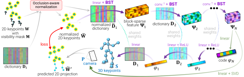
Figure 1: Deep NRSfM++ is a general framework for learning hierarchical block-sparse dictionaries that operates under perspective camera models with the ability to handle missing data. The 2D keypoint input $\mathbf{W}$ and shape dictionary $\mathbf{D}_{1}$ are normalized according to the visibility mask $\mathbf{M}$ and camera model (Table 1). The encoder-decoder network, derived from hierarchical block-sparse coding, takes the normalized 2D input $\widetilde{\mathbf{W}}$ and jointly predicts the camera matrix $\mathbf{P}$ and the 3D shape $\mathbf{S}$, further reprojected to 2D as $\widetilde{\mathbf{W}}^{\prime}$. The training objective is to minimize the difference between $\widetilde{\mathbf{W}}^{\prime}$ and $\widetilde{\mathbf{W}}$.

To solve the generalized bilinear factorization (7) given $N$ tuples of $(\mathbf{W}^{(n)},\mathbf{M}^{(n)})$ as the dataset (with $n$ indexing the samples), two problems remain to address: (i) how to define heuristics $\mathcal{C}$, which is crucial to have an accurate solution, and (ii) how to formulate the optimization strategy. We choose to follow Deep NRSfM [34], which instead of using simple handcrafted priors (e.g. low rank or sparsity), it imposes hierarchical sparsity constraint $\mathcal{C}_{\Theta}$ with learnable parameters $\Theta$ (see Sec. 4.1). The learning strategy of Deep NRSfM is then interpreted as solving a bilevel optimization problem:

where the lower level problems are to solve single frame 2D-3D lifting with given $\mathbf{D}$, $\Theta$; and the upper level problem is to find optimal $\mathbf{D}$,$\Theta$ for the whole dataset.

Descent method is employed to solve this bilevel problem. We first approximate the solver of the lower level problem as a feedforward network, i.e. $f(\mathbf{M},\mathbf{W}^{(n)};\mathbf{D},\Theta)\mapsto({\mathbf{R}^{*}}^{(n)}_{\mathbf{D},\Theta},{\boldsymbol{\varphi}^{*}}^{(n)}_{\mathbf{D},\Theta})$. The architecture of the network (as illustrated in Fig. 1) is induced from unrolling one iteration of Iterative Shrinkage and Thresholding Algorithm (ISTA) [7, 54, 27] (see Sec 4.2). Then with ${\mathbf{\Psi}^{*}}^{(n)}_{\mathbf{D},\Theta}={\boldsymbol{\varphi}^{*}}^{(n)}_{\mathbf{D},\Theta}\otimes{\mathbf{R}^{*}}^{(n)}_{\mathbf{D},\Theta}$, the original bilevel problem is reduced to a single level unconstrained problem, i.e.

which allows the use of solvers such as gradient descent. Finally, with $\mathbf{D},\Theta$ learned, $f(\mathbf{M},\mathbf{W};\mathbf{D},\Theta)$ is the 2D-3D lifting network applicable to unseen data.

Note: Due to the introduction of multiple levels of dictionaries and codes in Sec. 4.1, we will abuse the notation of $\mathbf{D}$, $\boldsymbol{\varphi}$, $\mathbf{\Psi}$ by adding subscript 1, i.e. $\mathbf{D}_{1}$, $\boldsymbol{\varphi}_{1}$, $\mathbf{\Psi}_{1}$ indicating that they are from the first level of the hierarchy.

4.1 Hierarchical Block-Sparse Coding (HBSC)

Assuming the canonical 3D shapes are compressible via multi-layer sparse coding, the shape code $\boldsymbol{\varphi}_{1}$ is constrained by $\mathcal{C}_{\Theta}$ as:

(18)

where $\mathbf{D}_{l}\in\mathbb{R}^{K_{l-1}\times K_{l}}$ are the hierarchical dictionaries, $l$ is the index of hierarchy level, and $\lambda_{l}$ is the scalar specifying the amount of sparsity in each level. Thus the learnable parameters for $\mathcal{C}_{\Theta}$ is $\Theta=\{\cdots,\mathbf{D}_{l},\lambda_{l},\cdots\}$. Constraints on multi-layer sparsity not only preserves sufficient freedom on shape variation, but it also results in more constrained code recovery.

Multi-layer sparse coding induces a hierarchical block sparsity constraint on the block codes $\mathbf{\Psi}_{l}$ (equal to $\boldsymbol{\varphi}_{l}\otimes\mathbf{R}_{xy}$ if orthogonal projection and $\boldsymbol{\varphi}_{l}\otimes\mathbf{R}$ if perspective), which leads to a relaxation of the lower level problem in (16):

where $\|.\|_{F}^{(3\times a)}$ denotes the sum of the Frobenius norm of each $3\times a$ block. Here, $a=2$ for orthogonal projections and $a=3$ for perspective projections.

Remark. Deep NRSfM [34] further relaxes the block sparsity in (19) to $L_{1}$ sparsity with a nonnegative constraint to allow for the use of ReLU activations in the network architecture. Such nonnegative constraint is inapplicable to our generalized formulation of $\mathbf{\Psi}$, and we empirically find the use of ReLU activation to degrade performance (Tab. 2).

4.2 HBSC-induced Network Architecture

The 2D-3D lifting network $f$ serves as an approximate solver of the HBSC problem (19). The architecture is induced from unrolling one iteration of the Iterative Shrinkage and Thresholding Algorithm (ISTA) [7, 54, 27], one of the classic methods for sparse coding. Unrolling iterative solver as network architecture has been widely practised to insert inductive bias for better generalization [53, 64, 58, 44, 29, 13, 46]. However, the motivation here is different – it is used to insert learnable priors to constrain an unsupervised learning problem. We provide derivations in the following.

Block soft thresholding. We review the block-sparse coding problem and consider the single-layer case. To reconstruct an input signal $\mathbf{X}$, we solves:

$$\min_{\mathbf{\Psi}}\|\mathbf{X}-\mathbf{D}\mathbf{\Psi}\|^{2}_{F}+\lambda\|\mathbf{\Psi}\|_{F}^{(3\times a)}\;.$$ (20)

One iteration of ISTA is computed as

$$\leavevmode\resizebox{399.2946pt}{}{$\displaystyle\mathbf{\Psi}^{(t+1)}=\text{prox}_{\lambda\|\cdot\|_{F}^{(3\times a)}}(\mathbf{\Psi}^{(t)}-\alpha\mathbf{D}^{\top}(\mathbf{D}\mathbf{\Psi}^{(t)}-\mathbf{X}))$}\;,$$ (21)

where $\text{prox}_{\lambda\|\cdot\|_{F}^{(3\times a)}}$ is the proximal operator for $L_{1}$ block sparsity of block size $3\times a$. Let $\mathbf{\Psi}=[\Pi_{1},\Pi_{2},\dots\Pi_{K}]^{\top}$, where $\Pi_{i}\in\mathbb{R}^{3\times a}\;\forall i$. Thus $\text{prox}_{\lambda\|\cdot\|_{F}^{(3\times a)}}$ is equivalent to applying block soft thresholding (BST) to all $\Pi_{i}$, defined as

$$\leavevmode\resizebox{399.2946pt}{}{$\displaystyle\text{BST}^{(3\times a)}(\mathbf{\Psi};\lambda)=\begin{bmatrix}\dots&(1-\frac{\lambda}{\|\Pi_{i}\|_{F}})^{+}\Pi_{i}^{\top}&\dots\end{bmatrix}^{\top}$}\;.$$ (22)

Assuming the block code $\mathbf{\Psi}$ is initialized to $\mathbf{0}$ with the step size $\alpha=1$, the first iteration of ISTA can be written as

$$\mathbf{\Psi}=\text{BST}^{(3\times a)}(\mathbf{D}^{\top}\mathbf{X};\lambda)\;.$$ (23)

We interpret BST as solving for the block-sparse code and incorporate $\text{BST}^{(3\times a)}(\cdot)$ as the nonlinearity in our encoder part of the network, similar to a single-layer ReLU network interpreted as basis pursuit [50]. Our formulation is closer to the true block-sparse coding objective than Deep NRSfM, which uses ReLU as the nonlinearity to relax the constraint to $L_{1}$ sparsity with nonnegative constraint.

Encoder-decoder network. By unrolling one iteration of block ISTA for each layer, our encoder takes $\widetilde{\mathbf{W}}$ as input and produces the block code for the last layer $\mathbf{\Psi}_{L}$ as output:

$$\mathbf{\Psi}_{1}= \text{BST}^{(3\times a)}\left([\widetilde{\mathbf{D}}_{1}^{\top}\widetilde{\mathbf{W}}]_{3K_{1}\times a};\boldsymbol{\lambda}_{1}\right),$$ (24)

$$\mathbf{\Psi}_{2}= \text{BST}^{(3\times a)}\left((\mathbf{D}_{2}\otimes\mathbf{I}_{3})^{\top}\mathbf{\Psi}_{1};\boldsymbol{\lambda}_{2}\right),$$

$$\vdots$$

$$\mathbf{\Psi}_{L}= \text{BST}^{(3\times a)}\left((\mathbf{D}_{L}\otimes\mathbf{I}_{3})^{\top}\mathbf{\Psi}_{L-1};\boldsymbol{\lambda}_{L}\right),$$

where $\boldsymbol{\lambda}_{l}$ is the learnable threshold for each $K_{l}$ block and $[\cdot]_{3K_{1}\times a}$ is a $3K_{1}\times a$ reshape. $(\mathbf{D}_{l}\otimes\mathbf{I}_{3})^{T}\mathbf{\Psi}_{l-1}$ are implemented by convolution transpose. $\mathbf{\Psi}_{L}$ are then factorized into $\boldsymbol{\varphi}_{L}$, $\mathbf{R}$ (constraining to $\mathbb{SO}(3)$ using SVD [34]). The 3D shape $\mathbf{S}$ is recovered from $\boldsymbol{\varphi}_{L}$ via the decoder as:

$$\boldsymbol{\varphi}_{L-1} =\text{ReLU}(\mathbf{D}_{L}\boldsymbol{\varphi}_{L}+\mathbf{b}_{L})\;,$$ (25)

$$\vdots$$

$$\boldsymbol{\varphi}_{1} =\text{ReLU}(\mathbf{D}_{2}\boldsymbol{\varphi}_{2}+\mathbf{b}_{2})\;,$$

$$\mathbf{S} =\mathbf{D}_{1}\boldsymbol{\varphi}_{1}\;.$$

Remark. Our key technical differences to Deep NRSfM are: (i) the first layer of the network is adaptive according to the camera model and keypoint visibility; (ii) replacement of ReLU with BST; (iii) block size of $\mathbf{\Psi}_{l}$ becomes $3\times 3$ under the perspective camera model.

5 Experiments

Architectural details. The most important hyperparameter of Deep NRSfM++ is the dictionary size $K_{L}$ at the last level, which depends on the shape variation that exhibits within the dataset. The rest are set arbitrarily and has less affect on performance. Setting $K_{L}$ to 8 gives reasonable result across all evaluated tasks. For optimal performance by validating on hold-out validation set, we use 8-10 for articulated objects and 2-4 for rigid ones. The detailed description of the architecture and the analysis of the robustness of $K_{L}$ are included in the Supp.

Shape scale $t_{z}$. To set the scale $t_{z}$ in practice, we make use of available 2D information such as bounding boxes; in applications where relative scales between samples in a dataset is available (e.g. human skeletons), we can utilize a strategy to estimate and recorrect the scale $t_{z}$ in an iterative fashion. We use the detected 2D object bounding box to provide an initial estimate of $t_{z}$ and subsequently update the scale estimation (using the Frobenius norm of $\mathbf{S}$ or the average bone length of a skeleton model, if available). Once we have updated the scale estimation $t_{z}$, we rerun Deep NRSfM++ and update the reconstruction. This scale correction procedure allows the 3D reconstruction and scale estimation to improve each other.

Evaluation metrics. We employ the following metrics to evaluate the accuracy of 3D reconstruction. MPJPE: before calculating the mean per-joint position, we normalize the scale of the prediction to match against ground truth (GT). To account for the ambiguity from weak perspective cameras, we flip the depth value of the prediction if it leads to lower error. PA-MPJPE: rigid align the prediction to GT before evaluating MPJPE. STRESS: borrowed from Novotny et al. [47] is a metric invariant to camera pose and scale. Normalized 3D error: 3D error normalized by the scale of GT, used in prior NRSfM works [5, 15, 34, 22].

Subject	CNS	NLO	SPS	Deep NRSfM	ReLU	BST
1	0.613	1.22	1.28	0.175	0.265	0.112
5	0.657	1.160	1.122	0.220	0.393	0.230
18	0.541	0.917	0.953	0.081	0.117	0.076
23	0.603	0.998	0.880	0.053	0.093	0.048
64	0.543	1.218	1.119	0.082	0.179	0.020
70	0.472	0.836	1.009	0.039	0.030	0.019
106	0.636	1.016	0.957	0.113	0.364	0.116
123	0.479	1.009	0.828	0.040	0.040	0.020

Table 2: 3D reconstruction error on CMU Motion Capture compared with NRSfM methods: CNS [43], NLO [16], SPS [33] and Deep NRSfM [34]. “ReLU” and “BST” are Deep NRSfM reimplemented with different nonlinearities.

BST vs ReLU. To study the effect of replacing ReLU with BST as the nonlinearity, we compare our approach against Deep NRSfM [34] on orthogonal projection data with perfect point correspondences on the CMU motion capture dataset [1]. Normalized 3D error is reported per human subject in Table 2. Our approach using BST achieves better accuracy compared to Deep NRSfM, providing empirical benefits of its closer proximity to solving the true block sparse coding objective.

Orthogonal projection with missing data. We evaluate Deep NRSfM++ on two benchmarks with high amount of missing data (Table. 3): (1) Synthetic UP-3D, a large synthetic dataset with dense human keypoints based on the UP-3D dataset [41]. The data was generated by orthographic projections of the SMPL body shape with the visibility computed from a ray tracer. We follow the same settings as C3DPO [47] and evaluate the 3D reconstruction of 79 representative vertices of the SMPL model on the test set. (2) PASCAL3D+ [69] consists of images of 12 rigid object categories with sparse keypoints annotations. To ensure consistency between 2D keypoint and 3D ground truth, we follow C3DPO and use the orthographic projections of the aligned CAD models with the visibility taken from the original 2D annotations. A single model is trained to account for all 12 object categories. We also include results where the 2D keypoints are detected by HRNet [57].

Method	MPJPE	STRESS
EM-SfM [60]	0.107	0.061
GbNRSfM [19]	0.093	0.062
Deep NRSfM [34]	0.076	0.063
C3DPO-base [47]	0.160	0.105
C3DPO [47]	0.067	0.040
Deep NRSfM++	0.062	0.037

(a) Test error on Synthetic UP-3D.

Method	MPJPE	STRESS
EM-SfM [60]	131.0	116.8
GbNRSfM [19]	184.6	111.3
Deep NRSfM [34]	51.3	44.5
C3DPO-base [47]	53.5	46.8
C3DPO [47]	36.6	31.1
Deep NRSfM++	34.8	27.9

(b) Test error on PASCAL3D+, where the input keypoints are from the ground truth.

Method	MPJPE	STRESS
Deep NRSfM [34]	65.3	47.7
CMR [32]	74.4	53.7
C3DPO [47]	57.5	41.4
Deep NRSfM++	53.0	36.1

(c) Test error on PASCAL3D+, where the input keypoints are off-the-shelf keypoint detection results from HRNet [57].

Table 3: Quantitative results on data generated by orthogonal projection with realistic occlusions.

Our method achieves over 32% error reduction over Deep NRSfM (Table 3(b)) while comparing favorably against other NRSfM methods and deep learning methods such as C3DPO.

Method	KSTA	CNS	Pose-GAN	C3DPO	Chen et al.	Deep NRSfM++
	[22]	[43]	[36]	[47]	[10]	ortho.	persp.	persp. +
								scale corr.
MPJPE	-	120.1	130.9	95.6	-	104.2	60.5	56.6
PA-MPJPE	123.6	79.6	-	-	58	72.9	51.8	50.9

(a) Test error on Human 3.6M compared against unsupervised methods. We report our results under both weak perspective and perspective camera models and demonstrate the effectiveness of applying scale corrections (2 iterations).

			w/o missing pts.		w/ missing pts.
method			train	test	train	test
CNS [43]			1.30	-	-	-
KSTA [22]			1.58	-	1.62	-
Deep	NRSfM++	ortho.	0.596	0.591	0.679	0.681
		persp.	0.152	0.145	0.182	0.185
		+ scale correction	0.131	0.124	0.165	0.168

(b) Test error on ApolloCar3D, where we report the MPJPE in meters as the evaluation metric.

Table 4: Quantitative results on real-world data with perspective projection.

Perspective projection. We evaluate our approach on two datasets with strong perspective effects: (1) Human 3.6M [30], a large-scale human pose dataset annotated by motion capture systems. We closely follow the commonly used evaluation protocol: we use 5 subjects (1, 5, 6, 7, 8) for training and 2 subjects (9, 11) for testing. (2) ApolloCar3D [55] has 5277 images featuring cars, where each car instance comes with annotated 3D pose. 2D keypoint annotations are also provided without 3D ground truth. To evaluate our method, we render 2D keypoints by projecting 34 car models according to the 3D pose labels. Visibility of each keypoints are marked according to the original 2D keypoint annotations. To showcase strong perspective effects, we select cars within 30 meters with no less than 25 visible points (out of 58 in total), which gives us 2848 samples for training and 1842 for testing.

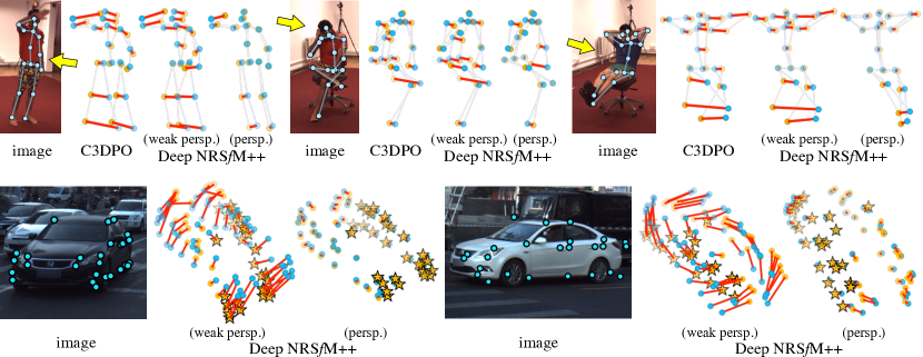
Figure 2: Qualitatative comparison. Blue points: GT, yellow points: prediction (stars indicate visible annotations), red lines: prediction error. The two rows are visual results from Human 3.6M and ApolloCar3D datasets respectively.

We evaluate different variants of our approach. We find that modeling perspective projection (Deep NRSfM++ persp.) leads to significant improvement over the orthogonal model (Deep NRSfM++ ortho.) and applying scale correction further improves accuracy. Deep NRSfM++ shows robustness under different level of noise and occlusion (see Table 6) and achieves the best result compared to other unsupervised learning method. We outperform the leading GAN-based method [10] by a significant margin when using the same training set (50.9 v.s. 58); in addition, Chen et al. [10] reaches our level of performance (50.9 vs 51) only when external training sources and temporal constraints are used. We provide qualitative results in Fig. 2, which shows the benefit of Deep NRSfM++’s ability to model perspective camera models while also outperforming C3DPO.

Noise	Missing pts. (%)
($\sigma$)	0	30	60
0	0.124	0.142	0.192
3	0.129	0.144	0.205
5	0.136	0.150	0.202
10	0.125	0.166	0.181
15	0.191	0.188	0.304

Table 5: Robustness with input under different occlusion rates and noises on ApolloCar3D.

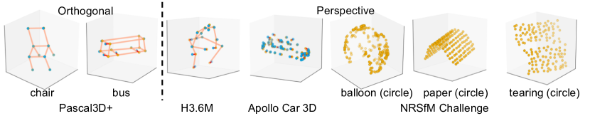
Table 6: Qualitative results across different datasets. Blue points: ground truth; yellow points and orange lines: reconstruction; red lines: difference between ground truth and reconstruction. Best viewed in color and zoomed in.

Deforming object in short sequences. Our method is applicable to NRSfM problems with limited number of frames. We experiment on NRSfM Challenge Dataset [31], which consists of 5 deforming objects captured with six different camera paths. While the leading methods all utilize trajectory information, our atemporal approach still gives reasonable reconstruction as shown in Fig. 6. The detailed comparison is in the supp. material.

6 Conclusion

We propose an atemporal approach applicable to SfC and unsupervised pose estimation. It provides an unified framework to model both orthogonal and perspective camera as well as missing data. The limitations of this work is: (i) the hierarchical sparsity prior is less robust to articulated objects when only limited number of frames is available (see Supp.). (ii) the connection between the proposed learning framework and the true objective of the NRSfM problem is still an approximation. Further theoritical investigation is in need to understand the benifit of this approximation or any possible alternatives, but is out of the scope of this paper.

I: Derivation for handling missing data under orthogonal camera.

To take possible occlusions into account, we have

$$\mathbf{M}\mathbf{W}=\mathbf{M}(\mathbf{S}\mathbf{R}_{xy}+\mathbf{1}_{P}\mathbf{t}_{xy}^{\top})\;.$$ (26)

where $\mathbf{M}=\text{diag}(m_{1},\cdots,m_{P})$ is a diagonal matrix indicating the visibility for each keypoints, $\mathbf{R}_{xy}$ is the first two columns in rotation matrix $\mathbf{R}$. By the object centric constraint, $\mathbf{t}_{xy}$ has the followin equation:

$$\mathbf{t}_{xy}=\frac{1}{P}\sum_{i=1}^{P}\underbrace{m_{i}\mathbf{w}_{i}}_{\text{visible points}}+\underbrace{(1-m_{i})(\mathbf{R}_{xy}^{\top}\mathbf{s}_{i}+\mathbf{t}_{xy})}_{\text{occluded points}},$$ (27)

where $m_{i}$ indicates the visibility of the $i$-th keypoint and $\mathbf{s}_{i}$ denotes the $i$-th 3D point in $\mathbf{S}$. Rearranging (27) yields an expression of $\mathbf{t}_{xy}$ with unknowns only from $\mathbf{R}_{xy}$, $\mathbf{S}$:

$$\mathbf{t}_{xy} =\frac{1}{\tilde{P}}\sum_{i=1}^{P}m_{i}\mathbf{w}_{i}+(1-m_{i})\mathbf{R}_{xy}^{\top}\mathbf{s}_{i}$$

$$=\frac{1}{\tilde{P}}[\mathbf{M}\mathbf{W}+(\mathbf{I}_{P}-\mathbf{M})\mathbf{S}\mathbf{R}_{xy}]^{\top}\mathbf{1}_{P}\;,$$ (28)

where $\tilde{P}$ denotes the number of visible points. Substituting (6) into (26) and rearranging, we have

$$\footnotesize{\mathbf{M}(\mathbf{W}-\mathbf{1}_{P}\frac{\mathbf{1}_{P}^{\top}\mathbf{M}\mathbf{W}}{\tilde{P}})=\mathbf{M}(\mathbf{S}\mathbf{R}_{xy}+\mathbf{1}_{P}\frac{\mathbf{1}_{P}^{\top}(\mathbf{I}_{P}-\mathbf{M})\mathbf{S}\mathbf{R}_{xy}}{\tilde{P}})\;.}$$ (29)

Since $\mathbf{S}\mathbf{R}_{xy}=\mathbf{D}^{\sharp}(\boldsymbol{\varphi}\otimes\mathbf{R}_{xy})=\mathbf{D}^{\sharp}\mathbf{\Psi}$, we have

$$\footnotesize{\mathbf{M}\underbrace{(\mathbf{W}-\mathbf{1}_{P}\frac{\mathbf{1}_{P}^{\top}\mathbf{M}\mathbf{W}}{\tilde{P}}}_{\tilde{W}\text{: normalized 2D projection}})=\mathbf{M}\underbrace{(\mathbf{D}^{\sharp}+\mathbf{1}_{P}\frac{\mathbf{1}_{P}^{\top}(\mathbf{I}_{P}-\mathbf{M})\mathbf{D}_{1}^{\sharp}}{\tilde{P}})}_{\tilde{\mathbf{D}}\text{: normalized dictionary}}\mathbf{\Psi}}$$ (30)

II: Implementation details

Dictionary sizes.

The dictionary size in each layer of the block sparse coding is listed in Table 7. We tried two strategies to set the dictionary sizes: (i) exponentially decrease the dictionary size, i.e. 512, 256, 128, …, (ii) linearly decrease, i.e. 125, 115, 104, … . Both strategies give reasonably good results. However, the hack we need to perform is to pick the size of the first and last layer dictionaries. We find that the size of the first layer would not have a major impact on accuracy as long as it is sufficiently large. The major performance factor is the size of the last layer dictionary $K_{L}$. In principal, we shall pick $K_{l}$ by measuring the accuracy on a small holdout validation set with 3D ground truth. We admit that this may become a problem in practise when no validation information is available. Indeed, having a more generalizable solution compared to hyperparameter tuning would be of interest to not only this work but also many other NRSfM or unsupervised 3D pose lifting approaches, which is an important topic to explore in the future. For now, we rely on the robustness of our approach against different bottleneck dimensions, and the rest hyperparameters are set arbitrarily without tuning. Figure 3 shows the 3D accuracy with different bottleneck dimensions on CMU-Mocap subject 64. It shows optimal result at dimension around 8 and 10, and has reasonable result at both lower and higher dimensions.

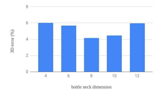
Figure 3: 3D reconstruction accuracy with different bottleneck dimensions on CMU-Mocap subject 64.

Training parameters.

We use Adam optimizer to train. Learning rate = 0.0001 with linear decay rate 0.95 per 50k iterations. The total number of iteration is 400k to 1.2 million depending on the data. Batch size is set to 128. Larger or smaller batch sizes all lead to similar result.

Initial scale for input normalization.

For weak perspective and strong perspective data, we need to estimate the scale so as to properly normalize the size of the 2D input shape. For Pascal3D+ and H3.6M datasets, we use the maximum length of the 2D bounding box edges, i.e. $t_{z}=1/\max(\text{bbox\_height, bbox\_width})$. For Apollo 3D Car dataset, we choose the minimum length of the bounding box, i.e. $t_{z}=1/\min(\text{bbox\_height, bbox\_width})$ by assuming that the height of each car is identical.

III: Additional empirical analysis

H3.6M.

We add the test result using detected 2D keypoint as input in Table 8. Deep NRSfM ++ achieves state-of-the-art result compared to other unsupervised methods.

ApolloCar3D.

Figure 4 shows additional analysis of Deep NRSfM ++ on the training set. Our method achieves $<25$cm error for over 80% testing samples with occlusions, while the compared baseline method, namely Consensus NRSfM [43] fails to produce meaningful reconstruction using perfect point correspondences. Average errors at different distances, rotation angles and occlusion rates are also reported. Overall, our method does not have a strong bias against a particular distance or occlusion rate. It does show larger error at $60^{\circ}$ azimuth, most likely due to the data distribution, where most cars are in either front ($\approx 0^{\circ}$) or back ($\approx 180^{\circ}$) view.

NRSfM Challenge Dataset.

The leading methods on the leaderboard all utilize temporal constraints, while our atemporal approach solves the problem only in the shape space. Therefore it is natural for our method to fall behind those methods, but nonetheless, we achieve reasonable results compared to other approaches also only use shape constraints. In Table 9 and Table 10, we compare to a selection of classical methods in literature. For a complete comparison, please refer to the official leaderboard of the challenge [31].

IV: Additional discussion

One of the benefit of solving NRSfM by training a neural network is that, in addition to 2D reconstruction loss, we can easily employ other loss functions to further constrain the problem. In summary, our preliminary study finds that: (i) adding the canonicalization loss [47] does not noticeably improve result. (ii) adding Lasso regularization on $\boldsymbol{\varphi}_{1}$ gives marginally better result in some datasets. (iii) adding symmetry constraint on the skeleton bone length helps to improve robustness against network initialization, but does not lead to noticeable better accuracy.

dataset	dictionary sizes
CMU-Mocap	512, 256, 128, 64, 32, 16, 8
UP3D	512, 256, 128, 64, 32, 16, 8
Pascal3D+	256, 128, 64, 32, 16, 8, 4, 2
H3.6M	125, 115, 104, 94, 83, 73, 62, 52, 41, 31, 20, 10
NRSfM Challenge	125, 115, 104, 94, 83, 73, 62, 52, 41, 31, 20, 10
Apollo	128, 100, 64, 50, 32, 16, 8, 4

Table 7: Dictionary sizes used in each reported experiment.

Method	MV/T	E3D	MPJPE	PA-MPJPE
Martinez et al. [45]	-	-	62.9	52.1
Zhao et al. [71]	-	-	57.6	-
3DInterpreter [68]		✓	-	98.4
AIGN [18]		✓	-	97.2
Tome et al. [59]	✓	✓	88.4	-
RepNet [63]		✓	89.9	65.1
Drover et al. [17]		✓	-	64.6
Pose-GAN [36]			173.2	-
C3DPO [47]			145.0	-
Wang et al. [65]			83.0	57.5
Chen et al. [10]	✓		-	68
Ours(persp proj)			68.9	59.4
+ scale corr itr1			67.3	59.2
+ scale corr itr2			67.0	58.7

Table 8: Result on H3.6M dataset with detected 2D kepoint input. In our result, we use detected points from cascaded pyramid network (CPN [11]) which is finetuned on H3.6M training set (excluding S9 and S11) by [52].

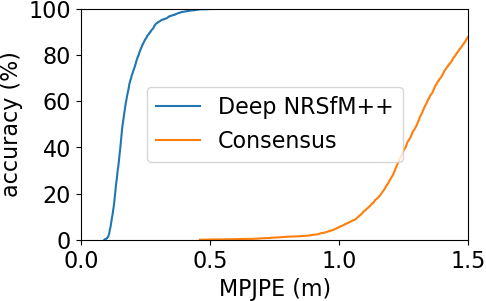
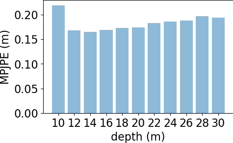
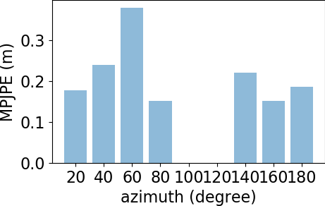
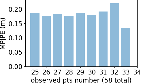
Figure 4: Additional result on Apollo 3D Car dataset. Top-left: percentage of sucess at different error thresholds. Rest: average error at different distances to the camera (top-right), azimuth angles of the car (bottom-left) and number of observed keypoints (bottom-right).

	temporal	Articulated	Balloon	Paper	Stretch	Tearing
CSF2	$\checkmark$	35.51	19.01	33.95	23.22	18.77
KSTA	$\checkmark$	42.11	18.45	32.18	22.88	17.59
PTA	$\checkmark$	36.71	28.88	41.72	30.45	23.14
Bundle	$\checkmark$	64.48	36.40	41.64	36.64	28.73
SoftInext	x	61.43	36.75	47.41	45.56	37.87
Compressible	x	72.77	52.53	62.44	57.45	54.71
MDH	x	88.66	58.27	66.98	66.27	56.67
Ours	x	47.80	30.16	44.33	36.59	30.74

Table 9: Comparison on NRSfM Challenge Dataset with orthogonal projection and no missing data.

	temporal	Articulated	Balloon	Paper	Stretch	Tearing
CSF2	✓	49.75	29.14	38.07	33.07	26.09
KSTA	✓	44.49	27.94	36.06	29.23	23.01
PTA	✓	58.08	37.20	47.42	41.40	30.96
Bundle	✓	58.95	37.07	40.88	38.16	27.40
SoftInext	x	69.11	41.76	53.91	48.98	45.93
Compressible	x	88.00	55.21	67.44	63.11	53.93
MDH	x	91.55	58.00	66.54	62.49	53.93
Ours	x	65.93	31.91	41.03	47.61	38.98

Table 10: Comparison on NRSfM Challenge Dataset with Perspective projection and no missing data.

References

- [1] Cmu motion capture dataset. available at http://mocap.cs.cmu.edu/.
- [2] A. Agudo and F. Moreno-Noguer. Recovering pose and 3d deformable shape from multi-instance image ensembles. In Asian Conference on Computer Vision, pages 291–307. Springer, 2016.
- [3] A. Agudo, M. Pijoan, and F. Moreno-Noguer. Image collection pop-up: 3d reconstruction and clustering of rigid and non-rigid categories. In The IEEE Conference on Computer Vision and Pattern Recognition (CVPR), June 2018.
- [4] I. Akhter, Y. Sheikh, and S. Khan. In defense of orthonormality constraints for nonrigid structure from motion. In 2009 IEEE Conference on Computer Vision and Pattern Recognition, pages 1534–1541. IEEE, 2009.
- [5] I. Akhter, Y. Sheikh, S. Khan, and T. Kanade. Nonrigid structure from motion in trajectory space. In Advances in neural information processing systems, pages 41–48, 2009.
- [6] A. Bartoli, D. Pizarro, and M. Loog. Stratified generalized procrustes analysis. International journal of computer vision, 101(2):227–253, 2013.
- [7] A. Beck and M. Teboulle. A fast iterative shrinkage-thresholding algorithm with application to wavelet-based image deblurring. Citeseer.
- [8] C. Bregler. Recovering non-rigid 3d shape from image streams. Citeseer.
- [9] G. Cha, M. Lee, and S. Oh. Unsupervised 3d reconstruction networks. In Proceedings of the IEEE International Conference on Computer Vision, pages 3849–3858, 2019.
- [10] C.-H. Chen, A. Tyagi, A. Agrawal, D. Drover, R. MV, S. Stojanov, and J. M. Rehg. Unsupervised 3d pose estimation with geometric self-supervision. In The IEEE Conference on Computer Vision and Pattern Recognition (CVPR), June 2019.
- [11] Y. Chen, Z. Wang, Y. Peng, Z. Zhang, G. Yu, and J. Sun. Cascaded pyramid network for multi-person pose estimation. In Proceedings of the IEEE Conference on Computer Vision and Pattern Recognition, pages 7103–7112, 2018.
- [12] A. Chhatkuli, D. Pizarro, T. Collins, and A. Bartoli. Inextensible non-rigid structure-from-motion by second-order cone programming. IEEE transactions on pattern analysis and machine intelligence, 40(10):2428–2441, 2017.
- [13] N. Chodosh, C. Wang, and S. Lucey. Deep convolutional compressed sensing for lidar depth completion. In Asian Conference on Computer Vision, pages 499–513. Springer, 2018.
- [14] S. Christy and R. Horaud. Euclidean shape and motion from multiple perspective views by affine iterations. IEEE Transactions on Pattern Analysis and Machine Intelligence, 18(11):1098–1104, 1996.
- [15] Y. Dai, H. Li, and M. He. A simple prior-free method for non-rigid structure-from-motion factorization. International Journal of Computer Vision, 107(2):101–122, 2014.
- [16] A. Del Bue, F. Smeraldi, and L. Agapito. Non-rigid structure from motion using ranklet-based tracking and non-linear optimization. Image and Vision Computing, 25(3):297–310, 2007.
- [17] D. Drover, R. MV, C.-H. Chen, A. Agrawal, A. Tyagi, and C. Phuoc Huynh. Can 3d pose be learned from 2d projections alone? In The European Conference on Computer Vision (ECCV) Workshops, September 2018.
- [18] H.-Y. Fish Tung, A. W. Harley, W. Seto, and K. Fragkiadaki. Adversarial inverse graphics networks: Learning 2d-to-3d lifting and image-to-image translation from unpaired supervision. In The IEEE International Conference on Computer Vision (ICCV), Oct 2017.
- [19] K. Fragkiadaki, M. Salas, P. Arbelaez, and J. Malik. Grouping-based low-rank trajectory completion and 3d reconstruction. In Advances in Neural Information Processing Systems, pages 55–63, 2014.
- [20] Y. Gao and A. L. Yuille. Symmetric non-rigid structure from motion for category-specific object structure estimation. In European Conference on Computer Vision, pages 408–424. Springer, 2016.
- [21] I. Goodfellow, J. Pouget-Abadie, M. Mirza, B. Xu, D. Warde-Farley, S. Ozair, A. Courville, and Y. Bengio. Generative adversarial nets. In Advances in neural information processing systems, pages 2672–2680, 2014.
- [22] P. F. Gotardo and A. M. Martinez. Kernel non-rigid structure from motion. In 2011 International Conference on Computer Vision, pages 802–809. IEEE, 2011.
- [23] P. F. Gotardo and A. M. Martinez. Non-rigid structure from motion with complementary rank-3 spaces. In CVPR 2011, pages 3065–3072. IEEE, 2011.
- [24] J. C. Gower. Generalized procrustes analysis. Psychometrika, 40(1):33–51, 1975.
- [25] O. C. Hamsici, P. F. Gotardo, and A. M. Martinez. Learning spatially-smooth mappings in non-rigid structure from motion. In European Conference on Computer Vision, pages 260–273. Springer, 2012.
- [26] R. Hartley and R. Vidal. Perspective nonrigid shape and motion recovery. In European Conference on Computer Vision, pages 276–289. Springer, 2008.
- [27] T. Hastie, R. Tibshirani, J. Friedman, and J. Franklin. The elements of statistical learning: data mining, inference and prediction. The Mathematical Intelligencer, 27(2):83–85, 2005.
- [28] A. Heyden, R. Berthilsson, and G. Sparr. An iterative factorization method for projective structure and motion from image sequences. Image and Vision Computing, 17(13):981–991, 1999.
- [29] P. Hu and D. Ramanan. Bottom-up and top-down reasoning with hierarchical rectified gaussians. In Proceedings of the IEEE Conference on Computer Vision and Pattern Recognition (CVPR), June 2016.
- [30] C. Ionescu, D. Papava, V. Olaru, and C. Sminchisescu. Human3. 6m: Large scale datasets and predictive methods for 3d human sensing in natural environments. IEEE transactions on pattern analysis and machine intelligence, 36(7):1325–1339, 2013.
- [31] S. H. N. Jensen, A. Del Bue, M. E. B. Doest, and H. Aanæs. A benchmark and evaluation of non-rigid structure from motion. arXiv preprint arXiv:1801.08388, 2018.
- [32] A. Kanazawa, S. Tulsiani, A. A. Efros, and J. Malik. Learning category-specific mesh reconstruction from image collections. In Proceedings of the European Conference on Computer Vision (ECCV), pages 371–386, 2018.
- [33] C. Kong and S. Lucey. Prior-less compressible structure from motion. In Proceedings of the IEEE Conference on Computer Vision and Pattern Recognition, pages 4123–4131, 2016.
- [34] C. Kong and S. Lucey. Deep non-rigid structure from motion. In The IEEE International Conference on Computer Vision (ICCV), October 2019.
- [35] C. Kong, R. Zhu, H. Kiani, and S. Lucey. Structure from category: A generic and prior-less approach. In 2016 Fourth International Conference on 3D Vision (3DV), pages 296–304. IEEE, 2016.
- [36] Y. Kudo, K. Ogaki, Y. Matsui, and Y. Odagiri. Unsupervised adversarial learning of 3d human pose from 2d joint locations. arXiv preprint arXiv:1803.08244, 2018.
- [37] S. Kumar. Jumping manifolds: Geometry aware dense non-rigid structure from motion. In Proceedings of the IEEE Conference on Computer Vision and Pattern Recognition, pages 5346–5355, 2019.
- [38] S. Kumar. Non-rigid structure from motion: Prior-free factorization method revisited. In Winter Conference on Applications of Computer Vision (WACV 2020), 2020.
- [39] S. Kumar, Y. Dai, and H. Li. Multi-body non-rigid structure-from-motion. In 2016 Fourth International Conference on 3D Vision (3DV), pages 148–156. IEEE, 2016.
- [40] S. Kumar, Y. Dai, and H. Li. Monocular dense 3d reconstruction of a complex dynamic scene from two perspective frames. In Proceedings of the IEEE International Conference on Computer Vision, pages 4649–4657, 2017.
- [41] C. Lassner, J. Romero, M. Kiefel, F. Bogo, M. J. Black, and P. V. Gehler. Unite the people: Closing the loop between 3d and 2d human representations. In IEEE Conf. on Computer Vision and Pattern Recognition (CVPR), July 2017.
- [42] M. Lee, J. Cho, C.-H. Choi, and S. Oh. Procrustean normal distribution for non-rigid structure from motion. In Proceedings of the IEEE Conference on computer vision and pattern recognition, pages 1280–1287, 2013.
- [43] M. Lee, J. Cho, and S. Oh. Consensus of non-rigid reconstructions. In Proceedings of the IEEE Conference on Computer Vision and Pattern Recognition, pages 4670–4678, 2016.
- [44] Z. Liu, X. Li, P. Luo, C. C. Loy, and X. Tang. Deep learning markov random field for semantic segmentation. IEEE transactions on pattern analysis and machine intelligence, 40(8):1814–1828, 2017.
- [45] J. Martinez, R. Hossain, J. Romero, and J. J. Little. A simple yet effective baseline for 3d human pose estimation. In Proceedings of the IEEE International Conference on Computer Vision, pages 2640–2649, 2017.
- [46] C. Murdock, M. Chang, and S. Lucey. Deep component analysis via alternating direction neural networks. In Proceedings of the European Conference on Computer Vision (ECCV), pages 820–836, 2018.
- [47] D. Novotny, N. Ravi, B. Graham, N. Neverova, and A. Vedaldi. C3dpo: Canonical 3d pose networks for non-rigid structure from motion. In The IEEE International Conference on Computer Vision (ICCV), October 2019.
- [48] J. Oliensis and R. Hartley. Iterative extensions of the sturm/triggs algorithm: Convergence and nonconvergence. IEEE Transactions on Pattern Analysis and Machine Intelligence, 29(12):2217–2233, 2007.
- [49] M. Paladini, A. Del Bue, J. Xavier, L. Agapito, M. Stošić, and M. Dodig. Optimal metric projections for deformable and articulated structure-from-motion. International journal of computer vision, 96(2):252–276, 2012.
- [50] V. Papyan, Y. Romano, and M. Elad. Convolutional neural networks analyzed via convolutional sparse coding. The Journal of Machine Learning Research, 18(1):2887–2938, 2017.
- [51] S. Parashar, A. Bartoli, and D. Pizarro. Self-calibrating isometric non-rigid structure-from-motion. In Proceedings of the European Conference on Computer Vision (ECCV), pages 252–267, 2018.
- [52] D. Pavllo, C. Feichtenhofer, D. Grangier, and M. Auli. 3d human pose estimation in video with temporal convolutions and semi-supervised training. In Proceedings of the IEEE Conference on Computer Vision and Pattern Recognition, pages 7753–7762, 2019.
- [53] J. Rick Chang, C.-L. Li, B. Poczos, B. Vijaya Kumar, and A. C. Sankaranarayanan. One network to solve them all–solving linear inverse problems using deep projection models. In Proceedings of the IEEE International Conference on Computer Vision, pages 5888–5897, 2017.
- [54] C. J. Rozell, D. H. Johnson, R. G. Baraniuk, and B. A. Olshausen. Sparse coding via thresholding and local competition in neural circuits. Neural computation, 20(10):2526–2563, 2008.
- [55] X. Song, P. Wang, D. Zhou, R. Zhu, C. Guan, Y. Dai, H. Su, H. Li, and R. Yang. Apollocar3d: A large 3d car instance understanding benchmark for autonomous driving. In Proceedings of the IEEE Conference on Computer Vision and Pattern Recognition, pages 5452–5462, 2019.
- [56] P. Sturm and B. Triggs. A factorization based algorithm for multi-image projective structure and motion. In European conference on computer vision, pages 709–720. Springer, 1996.
- [57] K. Sun, B. Xiao, D. Liu, and J. Wang. Deep high-resolution representation learning for human pose estimation. arXiv preprint arXiv:1902.09212, 2019.
- [58] C. Tang and P. Tan. Ba-net: Dense bundle adjustment network. arXiv preprint arXiv:1806.04807, 2018.
- [59] D. Tome, C. Russell, and L. Agapito. Lifting from the deep: Convolutional 3d pose estimation from a single image. In The IEEE Conference on Computer Vision and Pattern Recognition (CVPR), July 2017.
- [60] L. Torresani, A. Hertzmann, and C. Bregler. Nonrigid structure-from-motion: Estimating shape and motion with hierarchical priors. IEEE transactions on pattern analysis and machine intelligence, 30(5):878–892, 2008.
- [61] T. Ueshiba and F. Tomita. A factorization method for projective and euclidean reconstruction from multiple perspective views via iterative depth estimation. In European conference on computer vision, pages 296–310. Springer, 1998.
- [62] S. Vicente and L. Agapito. Soft inextensibility constraints for template-free non-rigid reconstruction. In European conference on computer vision, pages 426–440. Springer, 2012.
- [63] B. Wandt and B. Rosenhahn. Repnet: Weakly supervised training of an adversarial reprojection network for 3d human pose estimation. In Proceedings of the IEEE Conference on Computer Vision and Pattern Recognition, pages 7782–7791, 2019.
- [64] C. Wang, H. K. Galoogahi, C.-H. Lin, and S. Lucey. Deep-lk for efficient adaptive object tracking. In 2018 IEEE International Conference on Robotics and Automation (ICRA), pages 627–634. IEEE, 2018.
- [65] C. Wang, C. Kong, and S. Lucey. Distill knowledge from nrsfm for weakly supervised 3d pose learning. In The IEEE International Conference on Computer Vision (ICCV), October 2019.
- [66] G. Wang, H.-T. Tsui, and Z. Hu. Structure and motion of nonrigid object under perspective projection. Pattern recognition letters, 28(4):507–515, 2007.
- [67] G. Wang, H.-T. Tsui, and Q. M. J. Wu. Rotation constrained power factorization for structure from motion of nonrigid objects. Pattern Recognition Letters, 29:72–80, 2008.
- [68] J. Wu, T. Xue, J. J. Lim, Y. Tian, J. B. Tenenbaum, A. Torralba, and W. T. Freeman. Single image 3d interpreter network. In European Conference on Computer Vision, pages 365–382. Springer, 2016.
- [69] Y. Xiang, R. Mottaghi, and S. Savarese. Beyond pascal: A benchmark for 3d object detection in the wild. In IEEE Winter Conference on Applications of Computer Vision, pages 75–82. IEEE, 2014.
- [70] J. Xiao and T. Kanade. Uncalibrated perspective reconstruction of deformable structures. In Tenth IEEE International Conference on Computer Vision (ICCV’05) Volume 1, volume 2, pages 1075–1082. IEEE, 2005.
- [71] L. Zhao, X. Peng, Y. Tian, M. Kapadia, and D. N. Metaxas. Semantic graph convolutional networks for 3d human pose regression. In The IEEE Conference on Computer Vision and Pattern Recognition (CVPR), June 2019.
- [72] Y. Zheng, Y. Kuang, S. Sugimoto, K. Astrom, and M. Okutomi. Revisiting the pnp problem: A fast, general and optimal solution. In Proceedings of the IEEE International Conference on Computer Vision, pages 2344–2351, 2013.
- [73] X. Zhou, M. Zhu, S. Leonardos, K. G. Derpanis, and K. Daniilidis. Sparseness meets deepness: 3d human pose estimation from monocular video. In Proceedings of the IEEE conference on computer vision and pattern recognition, pages 4966–4975, 2016.
- [74] Y. Zhu, D. Huang, F. De La Torre, and S. Lucey. Complex non-rigid motion 3d reconstruction by union of subspaces. In Proceedings of the IEEE Conference on Computer Vision and Pattern Recognition, pages 1542–1549, 2014.