THz graphene W-shaped three-port circulator with dynamical control

Abstract

We propose a new graphene-based THz circulator. It consists of a circular graphene resonator and three graphene nanoribbon waveguides of W-geometry placed on a dilectric substrate. Surface plasmon-polariton waves propagate in the waveguides. The nanoribbon excites in the resonator dipole resonance. Nonreciprocity of the device is defined by nonsymmetry of the conductivity tensor of the magnetized graphene. The circulator with the central frequency 7.5 THz has the bandwidth 4.25% for isolation -15 dB, insertion loss -2.5 dB. Applied DC magnetic field is 0.56T and Fermi energy of graphene $\epsilon_{F}=0.15$eV. The Fermi energy allows one to control dynamically the circulator responses.

Keywords Circulator, graphene, surface plasmons, THz.

1 INTRODUCTION

Three-port circulator is one of the most popular nonreciprocal devices in microwave technology due to its excellent electrical characteristics, simple structure and versatility in applications. Typically, such a device has a three-fold rotational symmetry with input port, output port and one decoupled port [1]. The ports are usually microstrip lines or rectangular metal waveguides. The theory of stripline and waveguide microwave circulators is well developed [2]. Circulators of different types for optical systems are also described in literature (see, for example, [3, 4]). The main function of circulators is protection of a source of signal from unwanted reflections in the circuit, directing the reflected signal to the decoupled port where a matched load is connected. They are used also as switches [5, 6], as wavelength multiplexers and demultiplexers [7, 8], in dispersion compensators [9], in sensors [10] and reflectometry [11].

The physical effects utilized to produce the circulation are nonreciprocal phase shift, Faraday effect, nonreciprocal TE - TM mode conversion in waveguides, edge-guided mode regime [12] and resonances of two counterrotating modes with different frequencies in circular resonators [2].

At microwaves, the circulators are usually designed by using ferrites described by nonsymmetrical permeability tensor $[\mu]$. At higher frequencies, the use of ferrites in nonreciprocal devices is limited because of their relatively high losses and limited saturation magnetisation, i.e. weak gyromagnetic effect [13, 14]. For millimeter wave region, the semiconductor and 2D electron gas materials [15] with nonsymmetrical permittivity $[\varepsilon]$ tensor have been suggested to overcome some drawbacks of ferrite materials.

There are several proposals of the circulators for photonic crystal technology which can be used in THz, infrared and optical regions [16, 17, 18]. An idea of nonreciprocal components and, in particular, circulators, where a magnetic system is not required, was suggested recently in [19] and [20]. In such devices the circulation effect is achieved due to spatial-temporal permittivity modulation or staggered commutation. However, from the point of view of working parameters these types of circulators still can not compete with the traditional ones.

Nonreciprocal properties of graphene under DC magnetic field have been demonstrated experimentally in Faraday rotation scheme [21]. Recently, it was shown that magnetized graphene due to nonsymmetry of the conductivity tensor $[\sigma]$ can also be used for circulator design in THz and infrared regions.

In this paper, we suggest a new type of graphene-based circulator for the THz region with W-geometry. This device has a very simple and compact structure with good features. The design of the W-circulator was previously suggested in photonic crystal [22].

The analytical description of the circulator in terms of the scattering matrix based on temporal couple mode theory and magnetic group theory, which is developed in this work, can serve for modelling complex THz circuits and systems as it is made in microwave circuitry. Extensive numerical simulations demonstrate a good correspondence with analytical results.

2 PROBLEM DESCRIPTION

A schematic representation of the three-port W-circulator is shown in Fig. 1. This circulator consists of a circular graphene resonator magnetized by a DC magnetic field normal to graphene layer and three waveguides with angular distance of 60^∘ between them. The graphene elements are placed on a two-layer dielectric substrate. One of the layers is silica $(SiO_{2})$ and the other one is silicon $(Si)$.

In Fig. 2a, 2b and 2c, we demonstrate the physical principle of functioning of circulator considering excitation of different ports. When the signal is injected in port 1, the standing dipole mode has its node in port 2. Therefore, this corresponds to the transmission from port 1 to port 3. The transmission from port 2 to port 1 and from port 3 to port 2 can be explained analogously.

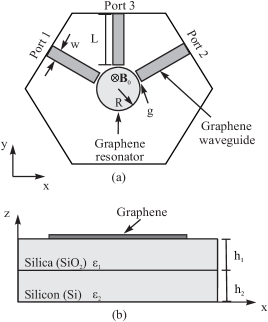
Figure 1: Geometry of W-circulator: a) top view, b) side view, B₀ is bias DC magnetic field.

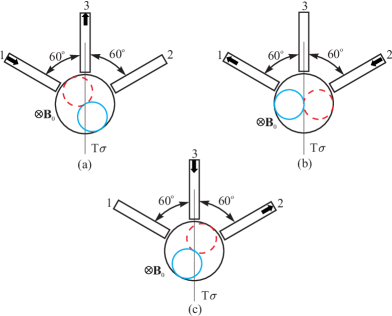
Figure 2: Excitation schemes of W-circulator with dipole mode (dotted and continuous circles) of resonator. Direction of circulation a) $1\rightarrow 3$, b) $2\rightarrow 1$, c) $3\rightarrow 2$ .

Using group theoretical description of the W-circulator [22] and considering the antiplane of symmetry $T\sigma$ (Fig. 2), the scattering matrix can be written in the following form:

$$S=\left(\begin{array}[]{ccc}S_{11}&S_{12}&S_{13}\\ S_{21}&S_{11}&S_{23}\\ S_{23}&S_{13}&S_{33}\end{array}\right)$$ (1)

where $S_{11}=S_{22}$, $S_{13}=S_{32}$ and $S_{23}=S_{31}$ are due to the antiplane of symmetry $T\sigma$. $S_{11}$ is the reflection coefficient at port 1, $S_{21}$ is the transmission coefficient from port 1 to port 2, $S_{31}$ is the transmission coefficient from port 1 to port 3, and so on. The per-cent fractional bandwidth of the device is defined as $BW=(f_{2}-f_{1})/f_{0}\times 100\%$, where $f_{2}$ and $f_{1}$ are the upper and lower frequency defined by the transmission level below -2.5 dB and the isolation level of the isolation port higher than -15 dB, $f_{0}$ is the central frequency of operation.

The device has the following dimensions: the length and width of the waveguides are $L=900$ nm and $w=120$ nm, respectively, the resonator radius $R=320$ nm, the gap between the waveguides and the resonator is $g=5$ nm. The dielectric layers of $SiO_{2}$ and $Si$ have the thicknesses $h_{1}=h_{2}=$ 2500 nm, with relative permittivity $\varepsilon_{1}=$ 2.09 and $\varepsilon_{2}=$ 11.9, respectively.

Our task is to analyze the properties of the circulator using the temporal coupled mode theory and numerical methods.

3 CONDUCTIVITY TENSOR

Surface conductivity of the magnetized graphene depends on radian frequency $\omega$, Fermi energy $\epsilon_{F}$, which is a function of electric biasing $E_{0}$, and also on the phenomenological scattering rate, defined as $\Gamma=1/\tau$, ($\tau$ is the relaxation time of graphene) and the cyclotron frequency $\omega_{B}={eB_{0}v_{F}^{2}}/{\epsilon_{F}}$, where $e$ is the electron charge, $v_{F}$ is the Fermi velocity, $B_{0}$ is DC magnetic field.

The tensor of the graphene conductivity [23] is:

$$[\sigma_{s}(\omega,\epsilon_{F}({E}_{0}),\Gamma,\omega_{B})]=\left[\begin{array}[]{cc}\sigma_{xx}&-\sigma_{xy}\\ \sigma_{xy}&\sigma_{xx}\\ \end{array}\right],$$ (2)

where $\sigma_{xx}=\sigma_{yy}$ and $\sigma_{yx}=-\sigma_{xy}$ are longitudinal (diagonal) and transverse (off-diagonal) parts, respectively. For the regime of intraband transitions in the THz region, they can be defined by the Drude formula [24]:

$$\sigma_{xx}=\frac{2D}{\pi}\frac{1/\tau-i\omega}{\omega_{B}^{2}-(\omega+i/\tau)^{2}},$$ (3)

$$\sigma_{xy}=-\frac{2D}{\pi}\frac{\omega_{B}}{\omega_{B}^{2}-(\omega+i/\tau)^{2}}.$$ (4)

where the Drude weight is given by $D=2\sigma_{0}\epsilon_{F}/\hbar$, $\hbar$ is the reduced Planck’s constant and $\sigma_{0}=e^{2}/(4\hbar)$ is the minimum conductivity of graphene. Fig. 3a and Fig. 3b show the frequency dependence of the real part and of the imaginary one of the tensor components of the graphene electrical conductivity. It can be observed that the cyclotron resonance frequency $\omega_{B}$ of the graphene is around 0.6 THz and that the imaginary part of the conductivity $\sigma_{xx}$ becomes negative above this frequency, which is necessary condition for the graphene device to support transverse magnetic (TM) surface plasmon polariton (SPP) waves. On the other hand, the real part of the conductivity, responsible for the graphene losses, increases rapidly in the vicinity of this frequency. So, to reduce losses in the circulator, the operating frequency of the device must be sufficiently higher than the cyclotron resonant frequency of the graphene.

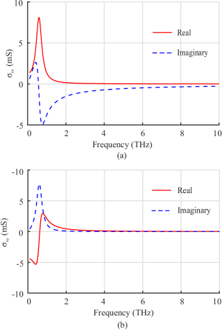
Figure 3: Real and imaginary parts of components $\sigma_{xx}$ ans $\sigma_{xy}$ of conductivity tensor of graphene, $B_{0}=0.56$ T, $\epsilon_{F}=0.15$ eV.

4 GRAPHENE NANORIBBON WAVEGUIDE

The numerical simulations were performed using the commercial software COMSOL Multiphysics version 5.2a [25], which is based on the Finite Element Method. Graphene has a very small thickness which can not be inserted directly in the modelling by the COMSOL software. To overcome this difficulty, we consider a monolayer with a finite thickness $\Delta$ and the conductivity tensor given by $[\sigma_{v}]=[\sigma_{s}]/\Delta$, where $[\sigma_{s}]$ is the tensor surface conductivity of graphene (2) given by components (3) and (4). In our numerical simulations we assume $\Delta=1$ nm. The artificial parameter $\Delta$ is used here only for calculation purposes [26] and numerical calculations were made for the following data: $\epsilon_{F}=0.15$ eV, $B_{0}=0.56$ T and $\tau=0.9$ ps [27].

In literature, the two main types of modes guided in graphene ribbons are discussed. One of them is concentrated around the center of the nanoribbon and other one at nanoribbon edges, both are known as surface plasmon polariton (SPP) modes [28, 29]. For our purposes, we choose the first mode which is shown in the insert of Fig. 4. In this figure, the dependence of the effective refractive index with respect to the width of the geraphene nanoribbon is presented.

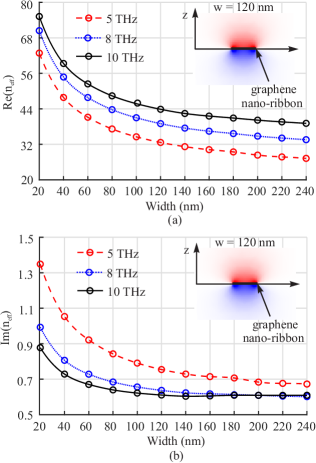
Figure 4: Width dependence mode of effective index for 5 THz, 8 THz, 10 THz. Insert is the $E_{z}$ profile of guided mode in the graphene strip.

5 RESONATOR RADIUS

The radius $R$ of the resonator for the lowest dipole mode can be estimated approximately from the condition $2\pi R=\lambda_{spp}$, where $\lambda_{spp}$ is the wavelength of the TM SPP mode. It is well known that the infinite graphene placed on an air-dielectric interface supports transverse-magnetic TM SPP waves with a dispersion relation given by:

$$\beta_{spp}=\dfrac{(1+\varepsilon_{1})(\omega\hbar)^{2}}{4\alpha\epsilon_{F}\hbar c}\biggl{(}1-\dfrac{\omega_{B}^{2}}{\omega^{2}}\biggr{)},$$ (5)

where $\alpha=e^{2}/(4\pi\varepsilon_{0}\hbar c)\approx 0.007$ is the fine-structure constant [30] and $c\approx 3\times 10^{8}$ m/s is the light velocity. Using the relations $R=\lambda_{spp}/2\pi$ and $\beta_{spp}=2\pi/\lambda_{spp}$, the radius of the resonator can be defined as follows:

$$R\approx A\dfrac{\epsilon_{F}}{(1+\varepsilon_{1})(\omega^{2}-\omega_{B}^{2})},$$ (6)

where $A=8.3\times 10^{40}(kg.m)^{-1}$, $\epsilon_{F}$ is Fermi energy given in $(J)$. As follows from (6), the radius of the resonator $R$ in $(m)$ is defined by the working frequency of the circulator $\omega$, cyclotron frequency of graphene $\omega_{B}$ given in (Hz), $\epsilon_{F}$ and by the permittivity of the substrate $\varepsilon_{1}$.

6 SIMULATION RESULTS

6.1 MAGNETIZED RESONATOR

Plasmonic waves are guided by graphene nanoribbons (see Fig 4). They excite dipole plasmonic resonance in the circular resonant graphene element. The SPP wave of the input waveguide excites in the circular resonator two degenerate clockwise $\omega_{+}$ and anticlockwise $\omega_{-}$ rotating modes. In Fig 5, the DC magnetic field $B_{0}$ dependence of the frequencies of the two rotating modes is shown. For the calculus, we use the model of only one exciting waveguide, one output waveguide and the resonant cavity (see insert in Fig 5). The splitting of the modes $\omega_{+}$ and $\omega_{-}$ increases with enlargement of $B_{0}$ almost linearly. The value of ${B}_{0}$ which provides at the central frequency of the circulator band the maximum of isolation, will be considered in the following discussion as an optimal DC magnetic field.

In Fig. 6 one can observe peaks of the transmission coefficient in 7.1 THz and 7.7 THz, corresponding to the dipole rotating modes with frequencies $\omega_{-}$ and $\omega_{+}$ and the quadrupole rotating modes in the interval from 9.5 THz to 10.2 THz. To calculate the Q-factor for the $\omega_{+}$ mode, we draw a line separating modes $\omega_{+}$ of the dipole and quadrupole resonances, because as can be seen, there is a superposition of these modes in the frequency range between them.

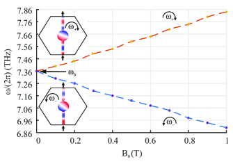
Figure 5: Magnetic DC field dependence of rotating mode resonances, $\epsilon_{F}=0.15$ eV. Insert: resonator feeding scheme for calculus of resonances.

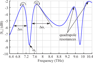
Figure 6: Frequency responses of resonant modes $\omega_{+}$ and $\omega_{-}$ for the feeding scheme shown in insert of Fig. 5. $B_{0}$ = 0.56 T, $\epsilon_{F}=0.15$ eV.

6.2 CIRCULATOR RESPONSES

For the case of the three-port without magnetization shown in Fig 7a, the sum of the counter-rotating modes produces a standing dipole, which leads to a transmission in both output ports. Magnetization by DC magnetic field breaks the degeneracy of the rotating modes and makes the field pattern of the standing wave to rotate by 30^∘ aligning thus the node of the dipole to port 2 and, therefore, isolating this port and transmitting the electromagnetic wave to port 3. Thus, if the signal is injected into port 1, it will be transmitted to port 3 with port 2 isolated. If the signal is injected in port 2, it is transmitted to port 1, isolating port 3. The same is true in the case of incidence in port 3: the signal is transmitted to port 2 and port 1 is isolated, as shown in Fig 7b, 7c, 7d, respectively.

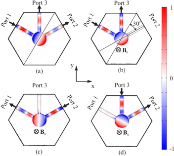
Figure 7: $E_{z}$ field profile for a) nonmagnetized case, and also for magnetized cases b) for transmission (1$\rightarrow$3), c) (2$\rightarrow$1) and d) (3$\rightarrow$2).

The frequency characteristics for the cases presented in Fig. 7b, 7c and 7d are shown in Fig. 8. For the case shown in 7c, the central frequency of operation is 7.5 THz, the device has the transmission coefficient of - 2 dB and isolation of -24.3 dB, presenting the bandwidth of 4.25% at the isolation level of -15 dB.

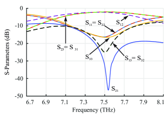
Figure 8: Frequency responses of circulator, $R$ = 320 nm, $g$ = 5 nm, $w$ = 120 nm, $B_{0}=0.56$ T, $\epsilon_{F}=0.15$ eV, excitation at port 1, 2 and 3.

Fig. 8 shows a comparison of the transmission, isolation and reflection curves of circulator, witch are in accordance with the symmetry analysis (see matrix (1)), where the isolations $S_{13}$ and $S_{32}$ are coincident, as well as the transmissions $S_{23}$ and $S_{31}$ and also the reflections $S_{11}$ and $S_{22}$. The peak of $S_{21}$ is higher and the curve $S_{21}$ presents a larger bandwidth with respect to the other two characteristics.

7 TEMPORAL COUPLED MODE THEORY OF CIRCULATOR

The temporal coupled mode theory (TCMT) [31] is based on very general assumptions such as weak coupling of the resonator with waveguides, linearity of the system, Time-reversal symmetry and energy conservation. It has been used in [32] to calculate characteristics of the Y-circulator. In the following, we use the theory developed in [33] for W-circulator.

In the following, we suppose, in the same way as in [32], that for the broken Time reversal symmetry, nonreciprocity of the device is defined only by the effect of the frequency splitting of the counter-rotating $\omega_{+}$ and $\omega_{-}$ of the resonator and the coupling coefficients between the waveguides and the resonator are reciprocal. The scattering matrix elements are defined as follows [33]:

$$S_{11}=S_{22}=S_{33}=-1+\frac{2}{3}\biggl{(}\frac{\gamma_{+w}}{\gamma_{+}+i(\omega-\omega_{+})}+\frac{\gamma_{-w}}{\gamma_{-}+i(\omega-\omega_{-})}\biggr{)},$$ (7)

$$S_{12}=\frac{2}{3}e^{-i2\varphi/3}\biggl{(}\frac{e^{i2\pi/3}\gamma_{+w}}{\gamma_{+}+i(\omega-\omega_{+})}+\frac{e^{-i2\pi/3}\gamma_{-w}}{\gamma_{-}+i(\omega-\omega_{-})}\biggr{)},$$ (8)

$$S_{32}=S_{13}=\frac{2}{3}e^{-i2\varphi/3}\biggl{(}\frac{e^{-i2\pi/3}\gamma_{+w}}{\gamma_{+}+i(\omega-\omega_{+})}+\frac{e^{i2\pi/3}\gamma_{-w}}{\gamma_{-}+i(\omega-\omega_{-})}\biggr{)},$$ (9)

$$S_{21}=\frac{2}{3}e^{i2\varphi/3}\biggl{(}\frac{e^{-i2\pi/3}\gamma_{+w}}{\gamma_{+}+i(\omega-\omega_{+})}+\frac{e^{i2\pi/3}\gamma_{-w}}{\gamma_{-}+i(\omega-\omega_{-})}\biggr{)},$$ (10)

$$S_{31}=S_{23}=\frac{2}{3}e^{i2\varphi/3}\biggl{(}\frac{e^{i2\pi/3}\gamma_{+w}}{\gamma_{+}+i(\omega-\omega_{+})}+\frac{e^{-i2\pi/3}\gamma_{-w}}{\gamma_{-}+i(\omega-\omega_{-})}\biggr{)},$$ (11)

where $\varphi=\varphi_{21}-\varphi_{32}$, $\varphi_{21}$ and $\varphi_{32}$ are phases of the elements $S_{21}$ and $S_{32}$, respectively. $\gamma_{+}=\gamma_{+w}+\gamma_{+i}$ and $\gamma_{-}=\gamma_{-w}+\gamma_{-i}$ are decay rates. Notice that $\gamma_{+w}$ and $\gamma_{-w}$ are decay rates due to coupling of the resonator with waveguides, and $\gamma_{+i}$ and $\gamma_{-i}$ due to internal losses of the resonator.

The resonance frequencies $\omega_{+}$, $\omega_{-}$ and the decay rates $\gamma_{+}$ and $\gamma_{-}$ were obtained from computational simulations for the scheme in the insert of Fig. 5. More specifically, the parameters of the TCMT $\omega_{+}$, $\omega_{-}$, $\gamma_{+}$ and $\gamma_{-}$ were obtained from the Comsol simulations shown in Fig. 6. The decay rate $\gamma_{+(_{-})}$ is related to the quality factor $Q_{+(_{-})}$, as $Q_{+(_{-})}=(3/2)\omega_{+(_{-})}/2\gamma_{+(_{-})}$. To compensate the difference in the number of ports of the devices (the three-port circulator and the two-port of Fig. 5), we multiplied the Q-factor by the constant 3/2. The obtained parameters are $\omega_{+}=48.38\times 10^{12}$ rad/s, $\omega_{-}=45.24\times 10^{12}$ rad/s, $\gamma_{+}\cong 3.4\times 10^{12}$ 1/s, $\gamma_{-}\cong 3.1\times 10^{12}$ 1/s. The parameters corresponding to internal losses of the resonator $\gamma_{+i}\cong 0.9\times 10^{12}$ 1/s and $\gamma_{-i}\cong 0.25\times 10^{12}$ 1/s, were used as fitting parameters to adjust the TCMT and the Comsol curves. The decay rates due to coupling of the resonator with waveguides are $\gamma_{+w}\cong 2.5\times 10^{12}$ 1/s and $\gamma_{-w}\cong 2.75\times 10^{12}$ 1/s.

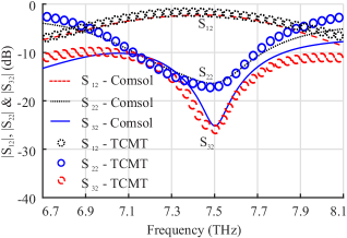
Figure 9: Frequency responses of circulator simulated by Comsol (continuous lines) and by TCMT (circles), $R$ = 320 nm, $g$ = 5 nm, $w$ = 120 nm, $B_{0}=0.56$ T, $\epsilon_{F}=0.15$ eV, excitation at port 2.

The theoretical results obtained by equations (7) - (11) and by software Comsol are shown in Fig. 9. We present only the results for the case of excitation applied at port 2, since similar results can be obtained for the excitation of ports 1 and 3. It can be seen that there is a good accordance between the two methods.

Similar to the photonic crystal W-circulator [33], the ideal circulator response with $S_{12}=1$ and $S_{32}=0$ ($\gamma_{+i}=\gamma_{-i}=0$) can be obtained at the central frequency of operation $\omega_{c}$. Bandwidth $BW$ for ideal circulator at the level of isolation -15 dB can be estimated by (9) and is defined by

$$BW=0.65\dfrac{(\omega_{+}-\omega_{-})}{\omega_{c}}100\%.$$ (12)

8 PARAMETRIC ANALYSIS OF CIRCULATOR

8.1 Varying the Radius of Resonator

The influence of the radius of the resonator on the resonance frequencies was investigated. The radius was changed from 220 nm to 470 nm and the other parameters as Fermi energy, width and gap were fixed at $\epsilon_{F}=0.15$ eV, $w=120$ nm, $g$ = 5 nm, respectively. Fig. 10 shows the frequency responses of the circulator corresponding to the radii of 220 nm, 270 nm, 370 nm and 470 nm. As can be seen from Fig. 11, the central frequency of the circulator is increased with decreasing the radius $R$ of the resonator. One can observe a systematic error of approximately 8% between the simulated results and those obtained by equation (6). This difference can be compensated including the multiplicative factor 1.08 in equation (6). One can also see in Fig. 12, that the optimal DC magnetic field $B_{0}$ decreases with increase of the resonator radius.

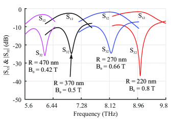
Figure 10: Frequency characteristics of circulator with different radii $R$, $g$ = 5 nm, $w$ = 120 nm, $\epsilon_{F}=0.15$ eV, excitation at port 2.

Figure 11: Central frequency of circulator versus radii $R$, $g$ = 5 nm, $w$ = 120 nm, $\epsilon_{F}=0.15$ eV. Numbers on the curve are DC magnetic field $B_{0}$, excitation at port 2.

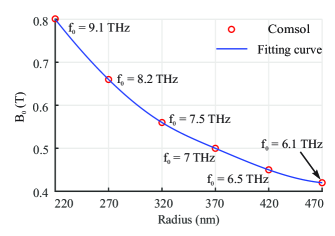
Figure 12: Optimal magnetic field of circulator for different radii $R$, $g$ = 5 nm, $w$ = 120 nm, $\epsilon_{F}=0.15$ eV. Numbers on the curve are central frequency ${f}_{0}$, excitation at port 2.

8.2 Influence of Waveguide Width

The influence of the width $w$ of the graphene waveguide on the resonance frequency and the insertion losses of the device was investigated as well. Varying the width from 120 nm to 240 nm we kept the other parameters fixed, i.e. $\epsilon_{F}=0.15$ eV, $R$ = 320 nm and $g$ = 5 nm. The frequency responses of the circulator are shown in Fig. 13. There is a shift of the resonance frequencies to higher values with increasing the width of the waveguide.

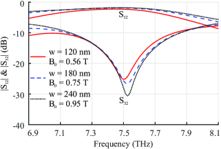
Figure 13: Frequency responses of circulator for different widths $w$, $g$ = 5 nm, $R=320$ nm, $\epsilon_{F}=0.15$ eV, excitation at port 2.

8.3 Gap Dependence of Circulator Characteristics

In this subsection, we show the influence of the gaps between the nanodisk and the waveguides on the central frequency of the circulator. The gaps was varied from 2.5 nm to 10 nm and the other parameters were fixed, i.e. $\epsilon_{F}=0.15$ eV, $R$ = 320 nm and $w$ = 120 nm. The frequency responses are plotted in Fig. 14 where one can see that the central frequency of operation of the device, the magnetic field and the bandwidth decrease with the increase of the gap (see Fig. 15, Fig. 16 and Fig. 17, respectively).

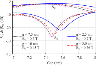
Figure 14: Frequency responses of circulator for different values of gap $g$, $w$ = 120 nm, $R=320$ nm, $\epsilon_{F}=0.15$ eV, excitation at port 2.

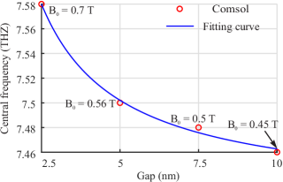
Figure 15: Central frequency of circulator for different values of gap $g$, $w$ = 120 nm, $R=320$ nm, $\epsilon_{F}=0.15$ eV. Numbers on the curve are DC magnetic field $B_{0}$, excitation at port 2.

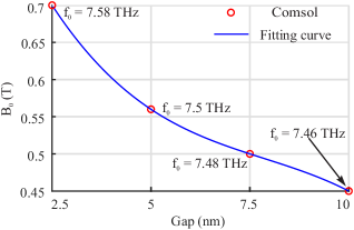
Figure 16: Gap $g$ dependence of optimal magnetic field of circulator, $w$ = 120 nm, $R=320$ nm, $\epsilon_{F}=0.15$ eV. Numbers on the curve are central frequency ${f}_{0}$, excitation at port 2.

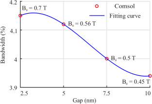
Figure 17: Bandwidth of circulator for different values of gap $g$; $w$ = 120 nm, $R=320$ nm, $\epsilon_{F}=0.15$ eV. Numbers on the curve are DC magnetic field $B_{0}$, excitation at port 2.

8.4 Control by Fermi Energy

To investigate the influence of the Fermi energy on the resonance frequencies, we varied $\epsilon_{F}$ from 0.1 eV to 0.3 eV. The frequency responses of the circulator are plotted in Fig. 18 from which it can be seen that the increase of the Fermi energy shifts the resonance frequency to higher values. Fig. 19 shows increase almost linearly of the optimal magnetic field $B_{0}$ with the increase of the Fermi energy. This is consistent with the formula $\omega_{B}={eB_{0}v_{F}^{2}}/{\epsilon_{F}}$.

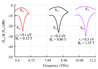
Figure 18: Frequency responses of the circulator, $g$ = 5 nm, $R$ = 320 nm, $w$ = 120 nm for different Fermi energies, excitation at port 2.

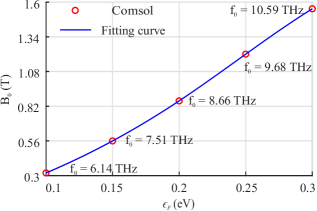
Figure 19: Fermi energy dependence of the optimal magnetic field $B_{0}$ for circulator, $g$ = 5 nm, $R$ = 320 nm, $w$ = 120 nm. Numbers on the curve give central frequency ${f}_{0}$, excitation at port 2.

To show a possibility to control dynamically the central frequency of the device, we keep all the parameters of the circulator fixed and change only the Fermi energy. Fig. 20 shows the shift of the central frequency of operation to the higher frequencies with increase of $\epsilon_{F}$ and this is consistent with (6). With a small change of $\epsilon_{F}$ between 0.12 eV and 0.18 eV, the central frequency varies from 6.8 THz to 8.1 THz ( $\pm 10$%). This leads also to small changes in the insertion losses and in the bandwidth of the device. Notice that in this case the DC magnetic field was fixed at $B_{0}=0.56$ T.

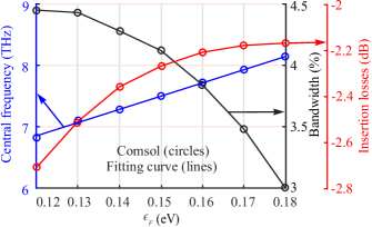
Figure 20: Illustration of dynamical control by Fermi energy: central frequency (blue circle), bandwidth (black circle) and of insertion losses (red circle), $B_{0}=0.56$ T, excitation at port 2.

9 CONCLUSIONS

We have suggested and confirmed by numerical simulations a realizability of controllable three-port graphene-based W-circulator operating in THz region. The temporal coupled mode theory was used for analysis of the circulator. The circulator presents a very simple structure consisting of graphene elements placed on a two-layer dielectric substrate. The central frequency of the circulator is defined mostly by the radius of the disc resonator. This frequency depends also on the graphene waveguide width, the gap between the resonator and the waveguides, the DC magnetic field and on the Fermi energy of graphene. The device simulations demonstrated that at the central frequency of 7.5 THz, its bandwidth is 4.25% with respect to the level of isolation -15 dB, and the insertion losses around -2 dB with the bias DC magnetic field $B_{0}=0.56$T and the Fermi energy of graphene $\epsilon_{F}=0.15$eV. We have shown that the central frequency of the circulator can be dynamically shifted by $\pm 10$% by an external electric field without significant deterioration of the circulator characteristics. The presented results can be useful in the projects of THz graphene circuits.

References

- [1] J. Helszain, “Waveguide Junction Circulators: Theory and Practice”, John Wiley Sons, New York, (1998).
- [2] J. Helszain, “The Stripline Circulators: Theory and Practice”, Wiley-IEEE Press, New Jersey, (2008).
- [3] V. Dmitriev, G. Portela, and L. Martins, “Three-port Circulators with Low Symmetry Based on Photonic Crystals and Magneto-Optical Resonators”, Photonic Network Communications, 31, 56-64, (2016).
- [4] Y. Wang, D. Zhang, S. Xu, B. Xu, Z. Dong, and Q. Xue, “Microwave-Frequency Experiment Validation of a Novel Magneto-Photonic Crystals Circulator”, IEEE Photonics Journal, 10, 1-6, (2018).
- [5] A. M. Kroening, “Advances in Ferrite Redundancy Switching for Ka-Band Receiver Applications”, IEEE Transactions on Microwave Theory and Techniques, 64, 1911-1917, (2016).
- [6] M. M. Biedka, R. Zhu, Q. M. Xu, and Y. E. Wang, “Ultra-Wide Band Non-Reciprocity Through Sequentially-Switched Delay Lines”, Scientific Reports, 7, 40014-40029, (2017).
- [7] J. Kim, and B. Lee, “Bidirectional Wavelength Add-Drop Multiplexer Using Multiport Optical Circulators and Fiber Bragg”, IEEE Photonics Technology Letters, 12, 561-563, (2000).
- [8] N. Reiskarimian, J. Zhou, and H. Krishnaswamy, “A CMOS Passive LPTV Nonmagnetic Circulator and Its Application in a Full-Duplex Receiver”, IEEE Journal of Solid-State circuits, 52, 1358-1372, (2017).
- [9] K. O. Hill, F. Bilodeau, B. Malo, T. Kitagawa, S. Thériault, D. C. Johnson, J. Albert, and K. Takiguchi, “Chirped In-Fiber Bragg gratings for Compensation of optical-fiber dispersion”, Optics Letters, 19, 1314-1316, (1994).
- [10] H. Zhang, J. Jiang, S. Liu, H. Chen, X. Zheng, and Y. Qiu, “Overlap Spectrum Fiber Bragg Grating Sensor Based on Light Power Demodulation”, Sensors, 18, 1597-1607, (2018).
- [11] N. Hayashi, Y. Mizuno, and K. Nakamura, “Alternative Implementation of Simplified Brillouin Optical Correlation-Domain Reflectometry”, IEEE Photonics Journal, 6, 1-8, (2014).
- [12] P. D. Santis, and F. Pucci, “The Edge-Guided-Wave Circulator”, IEEE Transactions on Microwave Theory and Techniques, 23, 516-519, (1975).
- [13] B. Lax, and K. J. Button, “Microwave Ferrites and Ferrimagnetics”, New York, NY, USA: McGraw-Hill, (1962).
- [14] A. Geiler, and V. Harris, “Atom magnetism: Ferrite Circulators-Past, Present, and Future”, IEEE Microwave Magazine, 15, 66-72, (2014).
- [15] A. Gabbay, and I. Brener, “Theory and Modeling of Electrically Tunable Metamaterial Devices Using Inter-Subband Transitions in Semi-conductor Quantum Wells”, Optics Express, 20, 6584-6597, (2012).
- [16] F. Fan, S. J. Chang, C. Niu, Y. Hou, and X. H. Wang, “Magnetically Tunable Silicon-Ferrite Photonic Crystals for Terahertz Circulator, Optics Communications, 285, 3763-3769, (2012).
- [17] W. Śmigaj, J. Romero-Vivas, B. Gralak, L. Magdenko, B. Dagens, and M. Vanwolleghem, “Magneto-Optical Circulator Designed for Operation in a Uniform External Magnetic Field”, Optics Letters, 35, 568-570, (2010).
- [18] K. Yayoi, K. Tobinaga, Y. Kaneko, A. V. Baryshev and M. Inoue, “Optical Waveguide Circulators Based on Two-Dimensional Magneto Photonic Crystal: Numerical Simulation for Structure Simplification and Experimental Verification”, Journal of Applied Physics, 109, 07B750, (2011).
- [19] N. A. Estep, D. L. Sounas, and A. Alu, “Magnetless Microwave Circulators Based on Spatiotemporally Modulated Rings of Coupled Resonators”, IEEE Transactions on Microwave Theory and Techniques, 64, 502-518, (2016).
- [20] N. Reiskarimian, and H. Krishnaswamy, “Magnetic-Free Non-Reciprocity Based on Staggered Commutation”, Nature communications, 7, 11217-11226, (2016)
- [21] A. Ferreira, J. V. Gomes, Y. V. Bludov, V. Pereira, N. M. R. Peres, and A. H. Castro Neto, “Faraday effect in graphene enclosed in an optical cavity and the equation of motion method for the study of magneto-optical transport in solids”, Physical Review B, 84, 235410-235435, (2011).
- [22] V. Dmitriev, M. N. Kawakatsu, and F. J. M. Souza, “Compact Three-Port Optical Two-Dimensional Photonic Crystal-Based Circulator of W-Format”, Optics Letters, 37, 3192-3194, (2012).
- [23] L. Giampiero, H. W. George, A. Rodolfo, and B. Paolo, “Semiclassical Spatially Dispersive Intraband Conductivity Tensor and Quantum Capacitance of Graphene”, Physical Review B, 87, 115429-115440, (2013).
- [24] Y. V. Bludov, A. Ferreira, N. M. R. Peres, and M. I. Vasilevskiy, “A Primer on Surface Plasmon-Polarintons in Graphene”, International Journal of Modern Physics B, 27, 1341001-1341075, (2013).
- [25] http://www.comsol.com.br
- [26] A. Vakil, and N. Engheta, “Transformation Optics Using Graphene”, Science, 332, 1291-1294, (2011).
- [27] A. Principi, and G. Vignale, “Intrinsic Lifetime of Dirac Plasmons in Graphene”, Physics Review B, 88, 195405-195420, (2013).
- [28] A. Y. Nikitin, F. J. Guinea, G. Vidal, and L. M. Moreno, “Edge and Waveguide Terahertz Surface Plasmon Modes in Graphene Microribbons”, Physical Review B, 84, 161-164, (2011).
- [29] S. He, X. Zhang, and Y. He, “Graphene Nano-Ribbon Waveguides of Record-Small Mode Area and Ultra-High Effective Refractive Indices for Future VLSI”, Optics express, 21, 30664-30673, (2013).
- [30] P. A. D. Gonçalves, and N. M. R. Peres, “An Introduction to Graphene Plasmonics”, World Scientific, New Jersey, (2016).
- [31] J. D. Joannopolus, S. G. Johnson, J. N. Winn, and R. D. Meade, “Photonic Crystals”, Princeton University Press, New Jersey, (2007).
- [32] Z. Wang, and S. Fan, “Magneto-Optical Defects in Two-Dimensional Photonic Crystals”, Apllied Physics B, Lasers and Optics, 81, 369-375, (2005).
- [33] V. Dmitriev, G. Portela, and L. Martins, “Temporal Coupled-Mode Theory of Electromagnetic Components Described by Magnetic Groups of Symmetry”, IEEE Transactions on microwave theory and techniques, 66, 1165-1171, (2018).