Hydrodynamic correlations of viscoelastic fluids by multiparticle collision dynamics simulations

Abstract

The emergent fluctuating hydrodynamics of a viscoelastic fluid modeled by the multiparticle collision dynamics (MPC) approach is studied. The fluid is composed of flexible, Gaussian phantom polymers, which interact by local momentum-conserving stochastic MPC collisions. For comparison, the analytical solution of the linearized Navier-Stokes equation is calculated, where viscoelasticity is taken into account by a time-dependent shear relaxation modulus. The fluid properties are characterized by the transverse velocity autocorrelation function in Fourier space as well as in real space. Various polymer lengths are considered—from dumbbells to (near-)continuous polymers. Viscoelasticity affects the fluid properties and leads to strong correlations, which overall decay exponentially in Fourier space. In real space, the center-of-mass velocity autocorrelation function of individual polymers exhibits a long-time tail independent of polymer length, which decays as $t^{-3/2}$, similar to a Newtonian fluid, in the asymptotic limit $t\to\infty$. Moreover, for long polymers an additional power-law decay appears at time scales shorter than the longest polymer relaxation time with the same time dependence, but negative correlations, and the polymer length dependence $L^{-1/2}$. Good agreement is found between the analytical and simulation results.

I Introduction

Soft matter and complex fluids are composed of a broad range of nano- to microscale objects. Such systems are typically easily deformable, with characteristic energies on the order of the thermal energy and correspondingly long relaxation times, and entropic degrees of freedom play an important role. Dhont et al. (2008); Menzel (2015); Nagel (2017) Paradigmatic examples of soft matter are biological cells—containing a wide range of polymeric and colloidal ingredients Ellis (2001); Bucciarelli et al. (2016)—blood, solutions of polymers, emulsions, and suspensions of colloidal particles. Bird, Armstrong, and Hassager (1987); Dhont (1996) The majority of these suspensions are viscoelastic rather than Newtonian, combining the viscous properties of fluids with elastic characteristics of solids. Ferry (1980); Bird et al. (1987); Bird, Armstrong, and Hassager (1987); Doi and Edwards (1986); Larson (1999)

Computer simulations are a valuable tool for gaining insight into the viscoelastic properties of complex fluids. Winkler, Fedosov, and Gompper (2014) Of particular interest are mesoscale simulation techniques, which account for hydrodynamic interactions and are able to bridge the length- and time-scale gap between fluid degrees of freedom and those of the embedded (polymeric) particles. Tao, Götze, and Gompper (2008); Kowalik and Winkler (2013) Established mesoscale techniques are the lattice Boltzmann method (LB), McNamara and Zanetti (1988); Shan and Chen (1993); Succi (2001); Dünweg and Ladd (2009) dissipative particle dynamics (DPD), Hoogerbrugge and Koelman (1992); Español and Warren (1995) and the multiparticle collision dynamics approach (MPC). Malevanets and Kapral (1999); Kapral (2008); Gompper et al. (2009) Viscoelasticity is incorporated in different ways in the various simulation approaches. LB describes a fluid in terms of a spatially discretized probability density, whose dynamics progresses via the Boltzmann equation. Succi (2001); Dünweg and Ladd (2009) Viscoelasticity is incorporated by extending the stress tensor by a viscous-stress contribution, e.g., the Maxwell model, Bird, Armstrong, and Hassager (1987); Ispolatov and Grant (2002); Dellar (2014) and taking this stress into account as a body force in the discretized propagation equation. Ispolatov and Grant (2002); Dellar (2014) In contrast, DPD and MPC are particle-based simulation approaches, where the bare fluid is represented by point particles, and a complex fluid by additional suspended objects such as colloids, polymers, membranes, or cells. In the latter approaches, viscoelasticity emerges as a consequence of the interactions between the embedded objects. Examples for viscoelastic DPD simulations are studies of blood cells Fedosov et al. (2011) and star polymers Fedosov et al. (2012) in flow. For MPC, the rheological properties of linear, branched, and star polymers Huang et al. (2010a); Nikoubashman and Likos (2010a); Singh et al. (2013); Winkler et al. (2013); Fedosov et al. (2012); Toneian (2019); Toneian, Likos, and Kahl (2019) have been investigated, as well as that of cells and vesicles. Noguchi and Gompper (2004)

Alternatively, viscoelastic fluids can be modeled by an ensemble of more complex entities, directly representing a viscoelastic fluid rather than a viscoelastic suspension. DPD and MPC viscoelastic fluids can be modeled by linearly connected DPD or MPC particles, respectively. The simplest viscoelastic unit is a dumbbell. The extension of the original DPD approach to a dumbbell fluid is presented in Ref. Somfai, Morozov, and van Saarloos, 2006 and to even longer polymers in Ref. Fedosov, Karniadakis, and Caswell, 2010. Similarly, the properties of MPC dumbbell fluids of different complexity are studied in Refs. Tao, Götze, and Gompper, 2008; Ji et al., 2011; Kowalik and Winkler, 2013; Toneian, 2015.

This representation of a viscoelastic fluid via an ensemble of linear elastic polymers raises a number of fundamental questions on hydrodynamic interactions in such a solution. Traditionally, it is assumed that hydrodynamic interactions are screened in polymer melts and that the properties of individual polymers in the melt are well described by the Rouse model. de Gennes (1979); Doi and Edwards (1986) Screening is assumed to emerge by the excluded-volume interactions between the polymers. Conversely, analytical considerations show that in melts of phantom polymers, i.e., polymers without excluded-volume interactions, hydrodynamic interactions are unscreened. Freed and Perico (1981)

Recent computer simulations and theoretical studies of unentangled polymer melts including excluded-volume interactions raise considerable doubts on this simple pictures, since the studies show clear evidence of a long-time tail in the polymer velocity correlation function, indicative for unscreened hydrodynamic interactions. Farago, Meyer, and Semenov (2011); Farago et al. (2012)

In this article, we study the properties of a viscoelastic fluid by analytical calculations and simulations. Our goal is to characterize the properties of the viscoelastic fluid, which will ultimately be used to study embedded objects. Analytically, we consider the linearized Navier-Stokes equations with a time-dependent relaxation modulus, i.e., an integro-differential equation for the velocity field. Bird, Armstrong, and Hassager (1987) The relaxation modulus follows from the Rouse model of polymer dynamics, Doi and Edwards (1986) a special case of the generalized Maxwell model. Bird, Armstrong, and Hassager (1987) In simulations, we employ the MPC approach, which has successfully been applied to study structural and dynamical properties of a wide range of polymeric systems. Mussawisade et al. (2005); Ryder and Yeomans (2006); Frank and Winkler (2008); Chelakkot, Winkler, and Gompper (2012); Nikoubashman and Likos (2010b); Huang et al. (2010a); Huang, Gompper, and Winkler (2013); Ripoll, Winkler, and Gompper (2006); Fedosov et al. (2012); Singh et al. (2014); Winkler, Fedosov, and Gompper (2014); Ghavami and Winkler (2017) It correctly captures hydrodynamic interactions Mussawisade et al. (2005); Huang, Gompper, and Winkler (2013) and can efficiently be parallelized on various platforms, especially on graphics processing units (GPUs). Westphal et al. (2014); Howard, Panagiotopoulos, and Nikoubashman (2018)

We analyze the fluid properties in terms of velocity autocorrelation functions. An analytical solution for the transverse velocity autocorrelation function is conveniently obtained in Fourier space, with respect to position, and in Laplace space, with respect to time. Inverse Laplace transformation yields a strongly time-dependent transverse autocorrelation function, which exhibits damped oscillations. Both, the damping and the oscillation frequencies depend on the relaxation times of the polymer and the wave vector. Independent of the polymer length, the (transverse) velocity autocorrelation function $C(t)$ exhibits a long-time tail on large length scales, with the time dependence $t^{-3/2}$ as is well established for Newtonian fluids. Felderhof (2005); Alder and Wainwright (1970); Zwanzig and Bixon (1970); Ernst, Hauge, and van Leeuwen (1971); Hauge and Martin-Löf (1973); Hinch (1975); Farago et al. (2012); Huang, Gompper, and Winkler (2012) Hence, hydrodynamic correlations determine the dynamical properties of a melt of phantom polymers on large length scales. This is reflected in the polymer center-of-mass diffusion coefficient, which exhibits the polymer length dependence according to the hydrodynamic Zimm model. Doi and Edwards (1986)

The article is organized as follows. Section II presents the polymer model and a description of the viscoelastic fluid in terms of a modified Navier-Stokes equation. Velocity autocorrelation functions of the fluid are introduced and their analytical solutions are presented in Sec. IV. The dynamics of the center-of-mass of an individual (tagged) polymer is discussed in Sec. V. Section III describes the MPC implementation, and Sec. VI presents the simulation results and a comparison with theoretical predictions. Finally, the main results and aspects of our study are summarized in Sec. VII. The Appendices A and B describe details of the calculation of inverse Laplace transformations. Appendix C illustrates the derivation of the center-of-mass velocity autocorrelation function of a tagged polymer.

II Model of Viscoelastic Fluid

II.1 Polymer Dynamics

We consider an ensemble of linear phantom polymers, each composed of $N$ monomers. The bonds between subsequent monomers are described by the harmonic Hamiltonian

$$H=\frac{K}{2}\sum_{i=1}^{N-1}\left(\bm{r}_{i+1}-\bm{r}_{i}\right)^{2}.$$ (2)

In the stationary state, this leads to a Gaussian partition function capturing the conformational degrees of freedom of the polymer. Winkler and Reineker (1992) The overdamped equation of motion for the position $\bm{r}_{i}(t)$ of monomer $i$, corresponding to the Rouse description of polymer physics, Doi and Edwards (1986); Harnau, Winkler, and Reineker (1997) is then

$$\dot{\bm{r}_{i}}=-\frac{1}{\gamma}\frac{\partial H}{\partial\bm{r}_{i}}+\frac{1}{\gamma}\bm{\varGamma}_{i}.$$ (3)

Here, $\dot{\bm{r}}_{i}(t)$ is the monomer velocity at time $t$, $k_{B}$ the Boltzmann constant, $T$ the temperature, $\gamma$ the friction coefficient, and the $\bm{\varGamma}_{i}$ represent stationary, Markovian, and Gaussian random processes with zero mean and the second moments ($\alpha,\beta\in\{x,y,z\}$)

$$\left\langle\varGamma_{i\alpha}(t)\varGamma_{j\beta}(t^{\prime})\right\rangle=2k_{B}T\gamma\delta_{ij}\delta_{\alpha\beta}\delta(t-t^{\prime}).$$ (4)

The coefficient $K$ in Eq. (2) is related to the mean square bond length $l^{2}$ via $K=3k_{B}T/l^{2}$.

The solution of Eq. (3) is Verdier (1966); Kopf, Dünweg, and Paul (1997)

$$\bm{r}_{i}(t)=\sum_{n=0}^{N-1}\bm{\chi}_{n}(t)b_{n}^{(i)},$$ (5)

with the eigenfunctions

$$b_{n}^{(i)}=\sqrt{\frac{2}{N}}\operatorname{cos}\left(\frac{n\pi}{N}\left[i-\frac{1}{2}\right]\right)$$ (6)

and

$$\bm{\chi}_{0}(t)=\sqrt{\frac{1}{2N}}\sum_{i=1}^{N}\bm{r}_{i}(t)=\sqrt{\frac{N}{2}}\bm{r}_{cm}.$$ (7)

The correlation functions of the mode amplitudes $\bm{\chi}_{n}$ are obtained as ($n,m\in\left[1,N-1\right]$)

$$\left\langle\bm{\chi}_{n}(t)\cdot\bm{\chi}_{m}(t)\right\rangle=\frac{l^{2}\delta_{nm}}{4\operatorname{sin}^{2}(n\pi/(2N))}e^{-t/\tau_{n}},$$ (8)

with the relaxation times

$$\tau_{n}=\frac{\gamma l^{2}}{12k_{B}T\operatorname{sin}^{2}(n\pi/2N)}.$$ (9)

In the continuum limit $N\to\infty$, $l\to 0$, such that $L=Nl$ remains constant, the well-know expression

$$\tau_{n}=\frac{\gamma L^{2}}{3\pi^{2}k_{B}Tn^{2}}=\frac{\tau_{R}}{n^{2}}$$ (10)

of the continuous Rouse model is obtained, with the Rouse relaxation time $\tau_{R}=\hat{\gamma}lL^{2}/3\pi^{2}k_{B}T$, the friction coefficient $\hat{\gamma}$ per length, and the bond length (Kuhn length) $l=2l_{p}$, where $l_{p}$ is the persistence length. Doi and Edwards (1986); Harnau, Winkler, and Reineker (1997)

The current formulation of the model, with $K=3k_{B}T/l^{2}$, applies to equilibrium systems only, and cannot reproduce some nonequilibrium properties, such as shear thinning. To capture such effects, the stretching of polymer bonds by the external forces needs to be prevented. In case of simple shear, this is easily achieved by a shear-dependent coefficient $\mu(\dot{\gamma})$ and the modified force coefficient $K=3\mu(\dot{\gamma})k_{B}T/l^{2}$, where $\dot{\gamma}$ is the shear rate. The coefficient $\mu$ follows from the inextensibility constraint $\sum_{i=1}^{N-1}\langle(\bm{r}_{i+1}-\bm{r}_{i})^{2}\rangle=(N-1)l^{2}$.Winkler (1999, 2010) More general, the constraint $\langle(\bm{r}_{i+1}-\bm{r}_{i})^{2}\rangle=l^{2}$ for every bond can be applied with a corresponding number of Lagrangian multipliers. Even for dumbbells, shear thinning is obtained with this length constraint. Kowalik and Winkler (2013)

II.2 Modified Navier-Stokes Equation

The viscous properties of Newtonian fluids are described by the Navier-Stokes equations. Landau and Lifshitz (1959) In the absence of external forces, the corresponding linearized equation for the fluid momentum is Landau and Lifshitz (1959)

$$\varrho\frac{\partial\bm{v}(\bm{r},t)}{\partial t}=-\nabla p+\eta\Delta\bm{v}(\bm{r},t),$$ (11)

with the fluid velocity $\bm{v}(\bm{r},t)$ and pressure $p(\bm{r},t)$ fields at the position $\bm{r}$ and time $t$, the fluid mass density $\varrho$, and the shear viscosity $\eta$. We want to consider a viscoelastic fluid composed of the phantom polymers of Sec. II.1. Viscoelasticity is incorporated in the Navier-Stokes equation by the (heuristic) extension Bird, Armstrong, and Hassager (1987); Ferry (1980)

$$\varrho\frac{\partial\bm{v}(\bm{r},t)}{\partial t}=-\nabla p+\int_{0}^{t}G(t-t^{\prime})\Delta\bm{v}(\bm{r},t^{\prime})dt^{\prime}.$$ (12)

Here, $G(t)$ is the shear relaxation modulus, which is independent of spatial coordinates and vanishes in the asymptotic limit $(t-t^{\prime})\to\infty$. Bird, Armstrong, and Hassager (1987)

The relaxation modulus $G^{p}(t)$ for the phantom polymers of Sec. II.1 has been determined in Ref. Doi and Edwards, 1986 as ($t\geq 0$)

$$G^{p}(t)=\varphi k_{B}T\sum_{n=1}^{N-1}e^{-2t/\tau_{n}},$$ (13)

where $\varphi$ is the number of polymers per volume. The latter is related with the mass density $\varrho$ via

$$\varphi=\frac{\varrho}{mN}=\frac{\phi}{N},$$ (14)

where $m$ is the monomer mass, and $\phi$ the overall monomer concentration. The complete fluid relaxation modulus $G(t)$ is, aside from the polymer-bond contribution, determined by the ideal gas contribution of the individual monomers due to their thermal motion. Hence, we use the relaxation modulus

$$G(t)=\eta\delta(t)+\varphi k_{B}T\sum_{n=1}^{N-1}e^{-2t/\tau_{n}}.$$ (15)

Then, the Navier-Stokes equation (12) reduces to that of a Newtonian fluid in case of a monomer solution ($N=1$).

The viscosity $\eta_{f}$ of the viscoelastic fluid follows from $G(t)$ via Doi and Edwards (1986)

$$\eta_{f}=\int_{0}^{\infty}G(t)dt,$$ (16)

which yields, with Eq. (10),Doi and Edwards (1986)

$$\eta_{f}=\eta+\frac{\varphi k_{B}T}{2}\sum_{n=1}^{N-1}\tau_{n}=\eta+\frac{\varphi\gamma l^{2}(N^{2}-1)}{36}.$$ (17)

With the density $\varphi$ of Eq. (14), the fluid viscosity becomes

$$\eta_{f}=\eta+\frac{\phi\gamma l^{2}}{36}\left(N-\frac{1}{N}\right).$$ (18)

For long polymers ($N\gg 1$) and fixed $\phi$, $\eta_{f}$ is dominated by the bond contribution ($G^{P}$) and $\eta$ is negligible. Then, the fluid viscosity increases linearly with the degree of polymerization, $N$.

III Mesoscale Hydrodynamics: Multiparticle Collision Dynamics

The MPC method for the simulation of polymer dynamics proceeds in two steps—streaming and collision. In the streaming step over a time interval $h$, where $h$ is denoted as collision time, Newton’s equations of motion for the monomers,

$$m\ddot{\bm{r}}_{i}=-\frac{\partial H}{\partial\bm{r}_{i}},$$ (19)

are solved by the velocity Verlet algorithm, Frenkel and Smit (2002) with the Hamiltonian of Eq. (2). Since we consider phantom polymers, only bond forces contribute to the monomer dynamics. Other monomer-monomer interactions are implemented via MPC collisions. Here, monomers are sorted into cubic cells of side length $a$, with the cells forming a complete tiling of the simulation volume, defining the collision environment. We apply the Stochastic Rotation Dynamics (SRD) Malevanets and Kapral (1999); Ihle and Kroll (2001); Kapral (2008) version of MPC, Gompper et al. (2009) where the relative monomer velocities, with respect to the center-of-mass velocity of all monomers in a collision cell, are rotated around a randomly oriented axis by a fixed angle $\alpha$. This yields the new monomer velocities

$$\bm{v}_{i}(t+h)=\bar{\bm{v}}_{i}(t+h)+\left(\mathrm{\bf R}(\alpha)-\mathrm{\bf E}\right)\left(\bar{\bm{v}}_{i}-\bar{\bm{v}}_{\textrm{cm}}^{c}\right),$$ (20)

where $\bar{\bm{v}}_{i}(t+h)$ is the monomer velocity after streaming, $\mathrm{\bf R}(\alpha)$ is the rotation matrix, $\mathrm{\bf E}$ the unit matrix, and

$$\bm{v}_{\textrm{cm}}^{c}(t)=\frac{1}{N_{c}}\sum_{j=1}^{N_{c}}\bm{v}_{j}(t)$$ (21)

is the center-of-mass velocity of the monomers in the cell of particle $i$; $N_{c}$ is the total number of monomers in that particular cell. The random orientation of the rotation axis is chosen independently for every collision step and every collision cell. Partitioning of the simulation volume into collision cells implies violation of Galilean invariance. To reestablish Galilean invariance, a random shift of the collision lattice is performed at every collision step.Ihle and Kroll (2001); Gompper et al. (2009) MPC conserves mass, momentum, and energy on the collision-cell level, which leads to correlations Ripoll et al. (2005); Tüzel, Ihle, and Kroll (2006) between the particles and long-range hydrodynamic interactions.Huang, Gompper, and Winkler (2012) To maintain a constant temperature, the Maxwell-Boltzmann-scaling (MBS) thermostat is applied at every collision step and for every collision cell.Huang et al. (2010b)

The simulations are performed with the hybrid program OpenMPCD, Toneian a software suite implementing MPC-SRD Malevanets and Kapral (1999, 2000); Gompper et al. (2009) combined with molecular dynamics simulations (MD) (velocity Verlet algorithm Frenkel and Smit (2002)). Both, the MPC and the MD part of the polymer dynamics—only phantom polymers with intramolecular bond interactions are considered—are executed in a massively parallel manner on a GPU (double precision). The program exhibits excellent performance on graphical processing units (GPUs) Westphal et al. (2014) supporting the CUDACUD (2015) programming framework, such as NVIDIA Tesla accelerators.

Dimensionless units are introduced by scaling length by the cell size $a$, energy by $k_{B}T$, and time by $\sqrt{ma^{2}/k_{B}T}$. This corresponds to the choice $a=k_{B}T=m=1$. We choose the collision time $h=0.1\sqrt{ma^{2}/k_{B}T}$, the rotation angle $\alpha=2.27\mathrm{rad}\approx 130^{\circ}$, and the mean number of monomers in a collision cell $\left\langle N_{c}\right\rangle=10$. The latter is equivalent with the mean fluid density $\varrho=10m/a^{3}$. A MD time step of $\Delta t=0.02\sqrt{ma^{2}/k_{B}T}$, smaller than the collision time step, is used in order to resolve the polymer dynamics adequately. Three-dimensional periodic systems are considered with a cubic simulation box of side length $L_{S}=30a$, if not indicated otherwise, corresponding to a total number of $N_{tot}=2.7\times 10^{5}$ monomers/MPC particles. Simulations of a monomer fluid, i.e., a bare MPC fluid, yield the viscosity $\eta/\sqrt{mk_{B}T/a^{4}}=8.7$. Huang et al. (2015) In the following, the units $a$, $k_{B}T$, and $m$ will be dropped, i.e., are set to unity. For the results presented in Sec. VI, between $2\times 10^{7}$ and $1\times 10^{8}$ MPC steps have been performed, typically approximately $4\times 10^{7}$.

Simulations are initialized by placing the first monomer of every polymer at a random point in the simulation volume sampled from a uniform distribution. Subsequent bound monomers are placed randomly by choosing a randomly oriented unit bond vector. Initial velocities of each monomer are assigned independently with Cartesian components taken from a standard normal distribution.

IV Velocity Correlation Function of Viscoelastic Fluid

The linear equation (12) can be solved using Fourier and Laplace transforms. Spatial Fourier transformation (denoted by a tilde) of the velocity,

$$\tilde{\bm{v}}(\bm{k},t)=\int\bm{v}(\bm{r},t)e^{-i\bm{k}\cdot\bm{r}}d^{3}r,$$ (22)

where $\tilde{\bm{v}}(\bm{k},t)$ denotes the transformed velocity, yields

$$\varrho\frac{\partial\tilde{\bm{v}}(\bm{k},t)}{\partial t}=-i\bm{k}{\tilde{p}}(\bm{k},t)-{\bm{k}}^{2}\int_{0}^{t}G(t-t^{\prime})\tilde{\bm{v}}(\bm{k},t^{\prime})dt^{\prime}.$$ (23)

By multiplying this equation with $\tilde{\bm{v}}(-\bm{k},0)$, we obtain ϱ∂~CT(k,t)∂t = - k^2 ∫_0^t G(t-t’)~C^T(k,t’) dt’ for the transverse velocity autocorrelation function ~C^T(k,t) = ⟨~v^T(k,t) ⋅~v^T(-k,0) ⟩, where the brackets denote statistical averaging. The transverse component $\tilde{\bm{v}}^{T}(\bm{k},t)$ is the component of the Fourier-space velocity $\tilde{\bm{v}}(\bm{k},t)=\tilde{\bm{v}}^{L}(\bm{k},t)+\tilde{\bm{v}}^{T}(\bm{k},t)$ that is perpendicular to the Fourier vector $\bm{k}$, i.e., $\bm{k}\cdot\tilde{\bm{v}}^{T}(\bm{k},t)=0$. Laplace transformation (denoted by a circumflex) with respect to time,

$$\hat{C}^{T}(\bm{k},s)=\int_{0}^{\infty}\tilde{C}^{T}(\bm{k},t)e^{-st}dt,$$ (24)

yields ^C^T(k,s) = ϱ~CT(k,0)ϱs + k2^G(s) . We assume that the system is in thermal equilibrium at $t=0$, hence, Huang, Gompper, and Winkler (2012)

$$\tilde{C}^{T}(\bm{k},0)\equiv\tilde{C}^{T}(0)=\frac{2k_{B}T}{\varrho}.$$ (25)

The Laplace transform of $G(t)$, Eq. (15), is Dyke (2014); Oberhettinger and Badii (2012) ^G(s) = η+ φk_BT ∑_n=1^N-1 1s + 2/τn , and we thus obtain ^C^T(k,s) = ϱ~CT(0)ϱs + k2(η+ φkBT ∑n=1N-11s + 2/τn) . The explicit expression $\tilde{C}^{T}(\bm{k},t)$ for the inverse Laplace transform of this function is presented in Eq. 62 of Appendix A.

The velocity correlation function $C(t)=\langle\bm{v}(\bm{r},t)\cdot\bm{v}(\bm{r},0)\rangle$ follows by inverse Fourier and Laplace transformation. To eliminate the spatial dependence, we average the correlation function with the distribution function for $\bm{r}(t)$. Alder and Wainwright (1970); Ernst, Hauge, and van Leeuwen (1971); Huang, Gompper, and Winkler (2012) Adopting the Lagrangian description of the fluid, where a fluid element is followed as it moves through space and time, we obtain in general

$$C(t) =\frac{1}{(2\pi)^{3}}\int\tilde{C}(\bm{k},t)\left\langle e^{i\bm{k}\cdot(\bm{r}(t)-\bm{r}(0))}\right\rangle\ d^{3}k$$

$$=\frac{1}{(2\pi)^{3}}\int\tilde{C}(\bm{k},t)e^{-\bm{k}^{2}\langle(\bm{r}(t)-\bm{r}(0))^{2}\rangle/6}\ d^{3}k,$$ (26)

due to the Gaussian nature of the displacement distribution function. Doi and Edwards (1986) The mean square displacement (MSD), averaged over all monomers, is Doi and Edwards (1986)

$$\left\langle\Delta\bm{r}(t)^{2}\right\rangle=\left\langle(\bm{r}(t)-\bm{r}(0))^{2}\right\rangle=6D_{\textrm{cm}}t+\left\langle\Delta\bm{r}(t)^{2}_{m}\right\rangle,$$ (27)

where $D_{\textrm{cm}}=k_{B}T/\gamma N$ is the center-of-mass diffusion coefficient, Doi and Edwards (1986) and with the results of Sec. II.1, we obtain the average monomer MSD in the polymer center-of-mass reference frame:

$$\left\langle\Delta\bm{r}(t)^{2}_{m}\right\rangle=\frac{l^{2}}{2N}\sum_{n=1}^{N-1}\frac{1}{\operatorname{sin}^{2}(n\pi/(2N))}\left(1-e^{-t/\tau_{n}}\right).$$ (28)

Examples of the correlation function $G(t)$ for various polymer lengths are discussed in the following.

IV.1 Newtonian Fluid ($N=1$)

A Newtonian fluid is recovered for $N=1$, and correspondingly $G(t)=\eta\delta(t)$. The inverse Laplace transformation of

$$\hat{C}^{T}(\bm{k},s)=\frac{\tilde{C}^{T}(0)}{s+\bm{k}^{2}\nu},$$ (29)

with the kinematic viscosity $\nu=\eta/\varrho$, yields the time-dependent velocity-correlation function in Fourier space, Oberhettinger and Badii (2012)

$$\tilde{C}^{T}(\bm{k},t)=\tilde{C}^{T}(0)e^{-\nu\bm{k}^{2}t},$$ (30)

in agreement with previous studies. Huang, Gompper, and Winkler (2012) With Eq. (25), the correlation function $C(t)=C^{L}(t)+C^{T}(t)$ of Eq. (26) becomes, in the long-time limit, Huang, Gompper, and Winkler (2012); Felderhof (2005); Alder and Wainwright (1970); Zwanzig and Bixon (1970); Ernst, Hauge, and van Leeuwen (1971)

$$C(t)\approx C^{T}(t)=\frac{k_{B}T}{4\varrho}\frac{1}{(\pi[\nu+D_{\textrm{cm}}]t)^{3/2}},$$ (31)

since the contribution of the longitudinal velocity correlation, $C^{L}(t)$, decays exponentially. Huang, Gompper, and Winkler (2012, 2013)

IV.2 Dumbbell fluid ($N=2$)

Polymer-like aspects are already captured by a dumbbell (dimer)—i.e., two bound monomers—at least as long as the longest relaxation time of a polymer dominates its internal dynamics. Here, Eq. 62 assumes the form

$$\tilde{C}^{T}(\bm{k},t)= \ \frac{\tilde{C}^{T}(\bm{k},0)}{\omega}e^{-\zeta t}$$ (32)

$$\times\left(\left[\frac{2}{\tau_{1}}-\zeta\right]\operatorname{sin}(\omega t)+\omega\operatorname{cos}(\omega t)\right),$$

with the abbreviations

$$\zeta= \ \frac{1}{2}\left(\frac{2}{\tau_{1}}+\bm{k}^{2}\nu\right),$$ (33)

$$\omega= \ \frac{1}{\tau_{1}}\sqrt{2\bm{k}^{2}\tau_{1}\left(\nu_{f}-\nu\right)-\frac{1}{8}\left(\bm{k}^{2}\nu\tau_{1}-2\right)^{2}},$$ (34)

and the kinematic viscosity $\nu_{f}=\eta_{f}/\varrho=\nu+\varphi k_{B}T\tau_{1}/(2\varrho)>\nu$. The correlation function (32) exhibits exponentially damped oscillations, where both the frequency, $\omega$, and the damping, $\zeta$, depend on the relaxation time $\tau_{1}$.

Evidently, the radicand in Eq. (34) is always negative for $\nu=\nu_{f}$. More general, in case of a negative radicand, the substitution $\omega=i\lambda$, with

$$\lambda=\frac{1}{\tau_{1}}\sqrt{-2\bm{k}^{2}\tau_{1}\left(\nu_{f}-\nu\right)+\frac{1}{8}\left(\bm{k}^{2}\nu\tau_{1}-2\right)^{2}},$$ (35)

yields the correlation function

$$\tilde{C}^{T}(\bm{k},t)= \ \frac{\tilde{C}^{T}(\bm{k},0)}{\lambda}e^{-\zeta t}$$ (36)

$$\times\left(\left[\frac{2}{\tau_{1}}-\zeta\right]\operatorname{sinh}(\lambda t)+\lambda\operatorname{cosh}(\lambda t)\right).$$

Since $\zeta>\lambda$, we obtain a non-oscillating correlation function. Equation (34), or Eq. (35), clearly reveal a qualitative different dynamical behavior due to polymer elasticity (viscoelasticity). An oscillatory correlation function function appears for $\nu_{f}>\nu$ only. There are two obvious limits with only exponentially decaying correlation functions, namely $|\bm{k}|\to 0$ and $|\bm{k}|\to\infty$, which correspond to large and small scales, respectively.

In the limit $\lambda t\gg 1$, Eq. (36) becomes

$$\tilde{C}^{T}(\bm{k},t)=\tilde{C}^{T}(\bm{k},0)\left(\frac{1}{\lambda\tau_{1}}-\frac{\zeta}{2\lambda}+\frac{1}{2}\right)e^{-(\zeta-\lambda)t}.$$ (37)

For $|\bm{k}|\to 0$, the difference in the exponent reduces to $\zeta-\lambda=\bm{k}^{2}(\nu+\varphi k_{B}T\tau_{1}/2\varrho)+O(\bm{k}^{4})$ (Eq. (17)), and the correlation function decays exponentially with the total kinematic viscosity, $\nu_{f}$,

$$\tilde{C}^{T}(\bm{k},t)=\tilde{C}^{T}(\bm{k},0)e^{-\nu_{f}\bm{k}^{2}t}.$$ (38)

Then, Fourier transformation w.r.t. $\bm{k}$ of Eq. (38) yields a long-time tail $C^{T}(t)\sim(\nu_{f}t)^{-3/2}$ on large length and long time scales. Conversely, on small length scales $|\bm{k}|\to\infty$, the exponent becomes $\zeta-\lambda=2(1+\nu_{f}/\nu)/\tau_{1}+O(1/\bm{k}^{2})$, and the decay of the correlation function depends only weakly on the wave vector. In both cases, the decline of $\tilde{C}^{T}(\bm{k},t)$ is determined by the properties of the dumbbell rather than the individual monomers.

Figure 1 provides examples of the correlation function $\tilde{C}^{T}(\bm{k},t)$ for various wave vectors and a specific set of parameters (see figure caption). Note that the oscillating correlation functions assume positive and negative values. The correlation functions for the smallest ($k=0.09$) and the largest ($k=2$) displayed $\bm{k}$ vectors decay exponentially according to Eq. (37), whereas those for in-between $\bm{k}$ values exhibit exponentially damped oscillations, Eq. (32). In the latter case, the oscillation frequency increases with increasing wave number. The decay rates in the limit $|\bm{k}|\to 0$ and $|\bm{k}|\to\infty$ agree with the values discussed above.

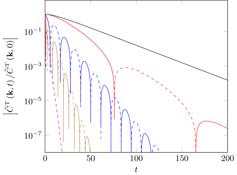
Figure 1: Transverse velocity autocorrelation function $\tilde{C}^{T}(\bm{k},t)/\tilde{C}^{T}(\bm{k},0)$ of dumbbells (Eq. (32) or (36)) as a function of time for the wave vectors $|\bm{k}|=0.09$, $0.11$, $0.4$, $0.8$, and $2$ (top to bottom). The other parameters are $\eta=8.7$, $\varrho=10$, $\varphi k_{B}T=5$, and $\tau_{1}=13.4$. Due to viscoelasticity, the correlation function oscillates for certain wave vectors assuming positive (solid) and negative (dashed) values.

IV.3 Continuous Polymer ($N\to\infty$)

In the case of continuous polymers, $N\to\infty$, the relaxation modulus (15) becomes

$$G(t)=\eta\delta(t)+\varphi k_{B}T\sum_{n=1}^{\infty}e^{-2tn^{2}/\tau_{R}}.$$ (39)

Two limiting case can be distinguished

• $t/\tau_{R}\gg 1$ — The sum in Eq. (39) is dominated by the mode $n=1$, corresponding to the dumbbell considered in Sec. IV.2 with the relaxation time $\tau_{1}=\tau_{R}$. Again, on large length scales, the velocity correlation function decays exponentially with the viscosity $\eta_{f}=\eta+\varphi k_{B}T\tau_{R}/2$, where $\eta$ can be neglected for long polymers due to the large Rouse time.

• $t/\tau_{R}\ll 1$ — The sum of modes in Eq. (39) can be replaced by an integral over $n$, Doi and Edwards (1986); Winkler, Keller, and Rädler (2006) and we straightforwardly obtain

  $$G(t)=\eta\delta(t)+\frac{\varphi k_{B}T}{2}\sqrt{\frac{\pi\tau_{R}}{2t}}.$$ (40)

  Laplace transformation yields

  $$\hat{G}(s)=\eta+\frac{\varphi k_{B}T\pi}{2}\sqrt{\frac{\tau_{R}}{2s}},$$ (41)

  and the velocity correlation function becomes

  $$\hat{C}^{T}(\bm{k},s)=\frac{\displaystyle\varrho\tilde{C}^{T}(\bm{k},0)}{\displaystyle\varrho s+\bm{k}^{2}\left(\eta+\frac{\varphi k_{B}T\pi}{2}\sqrt{\frac{\tau_{R}}{2s}}\right)}.$$ (42)

  Inverse Laplace transformation (cf. Appendix B) yields, neglecting $\eta$,

  $$\tilde{C}^{T}(\bm{k},t)={\tilde{C}}^{T}(0)f([\bm{k}^{2}\varphi k_{B}T\pi\sqrt{\tau_{R}}/(2\sqrt{2}\varrho)]^{2/3}t),$$ (43)

  with the function $f(x)$ specified in Eq. (69). Hence, $\tilde{C}^{T}(\bm{k},t)$ scales with $(k^{4/3}t)$ as already pointed out in Ref. Farago et al., 2012.

  In the asymptotic limit of a large argument of $f$ in Eq. (43), we find

  $$\tilde{C}^{T}(\bm{k},t)=-\frac{\sqrt{2}\varrho\,{\tilde{C}}^{T}(\bm{k},0)}{\varphi k_{B}T\pi\sqrt{\pi\tau_{R}}}\frac{1}{\bm{k}^{2}t^{3/2}}.$$ (44)

  Note that the correlation function is negative. The correlation function exhibits a long-time-tail-type time dependence $t^{-3/2}$, which is very different from the exponential function of Eq. (30) for individual monomers. Polymer elasticity complete changes the time and wave-vector dependence of the correlation function. However, as shown in Sec. V.1.2, this does not affect the long-time-type decay of the correlation function in real space.

  Inserting $\tilde{C}^{T}(\bm{k},0)$ of Eq. (25) and the polymer concentration of Eq. (14) into Eq. (44), we find

  $$\tilde{C}^{T}(\bm{k},t)=-\frac{2\sqrt{2}}{\pi^{3/2}\phi l\sqrt{\tau_{l}}}\frac{1}{\bm{k}^{2}t^{3/2}},$$ (45)

  with the abbreviation $\tau_{l}=\hat{\gamma}l/(3\pi^{2}k_{B}T)$. Thus, the fluid correlation function $\tilde{C}(\bm{k},t)$ is independent of polymer length in the time interval $\tau_{l}\ll t\ll\tau_{R}$ for long polymers ($L/l\gg 1$); it depends on the overall monomer density only.

IV.4 Asymptotic Behavior for $t\to\infty$

The asymptotic time dependence of the correlation function $C^{T}(t)$ for $t\to\infty$ follows from Eq. (IV) in the limit $s\to 0$. Neglecting $s$ in the sum over modes in Eq. (IV), the correlation function reduces to $\hat{C}^{T}(\bm{k},s)=\tilde{C}^{T}(0)/(s+\bm{k}^{2}\nu_{f})$, with the total kinematic viscosity $\nu_{f}=\eta_{f}/\varrho$. Then, Fourier and Laplace transformations yield

$$C^{T}(t)=\frac{\tilde{C}^{T}(0)}{8\left(\pi\nu_{f}t\right)^{3/2}}$$ (46)

independent of polymer length. This result is consistent with the limiting cases discussed in Secs. IV.1, IV.3, and corresponds to the long-time tail of simple fluids.Huang, Gompper, and Winkler (2012); Felderhof (2005); Alder and Wainwright (1970); Zwanzig and Bixon (1970); Ernst, Hauge, and van Leeuwen (1971) Hence, on large length scales and for long times, the polymer melt of phantom chains exhibits fluid-like behavior similar to simple fluids, but with the total viscosity $\eta_{f}$ determined by polymer elasticity.

IV.5 Oseen Tensor-Type Behavior

Integration of the correlation function ${\tilde{C}}^{T}(\bm{k},t)$ over time yields

$$T(k)=\int_{0}^{\infty}{\tilde{C}}^{T}(\bm{k},t)dt={\hat{C}}^{T}(\bm{k},0)=\frac{\varrho\tilde{C}^{T}(0)}{\bm{k}^{2}\eta_{f}},$$ (47)

with the use of the definition of the Laplace transform (24) and Eq. (IV). Hence, $T(k)\sim 1/\bm{k}^{2}$, similar to the Oseen tensor of a Newtonian fluid, Doi and Edwards (1986); Dhont (1996); Huang, Gompper, and Winkler (2012) but with the viscosity of the polymeric fluid. Fourier transformation with respect to $\bm{k}$ leads then to a long-range interaction $\sim 1/|\bm{r}|$ in three-dimensional space. As a consequence, the considered viscoelastic phantom polymer melt exhibits the properties of Newtonian fluids in terms of long-range fluid interactions.

V Center-of-Mass Dynamics of Individual Polymers

The equations of motion (3) describe the dynamics of an isolated polymer exposed to thermal noise. We now consider an individual polymer embedded in other, identical polymers, accounting for the environment by including the convective transport velocity following from Eq. (12). Hence, we set

$$\dot{\bm{r}}_{i}(t)=\bm{v}(\bm{r}_{i},t)-\frac{1}{\gamma}\frac{\partial H}{\partial\bm{r}_{i}}+\frac{1}{\gamma}{\bm{\varGamma}}_{i}(t),$$ (48)

with the fluid velocity $\bm{v}(\bm{r}_{i},t)$ at the location of monomer $i$. Considering the center-of-mass motion only, we find

$$\dot{\bm{r}}_{\textrm{cm}}(t)=\frac{1}{N}\sum_{i=1}^{N}\bm{v}(\bm{r}_{i},t)+\frac{1}{\gamma N}\sum_{i=1}^{N}{\bm{\varGamma}}_{i}(t),$$ (49)

for the position $\bm{r}_{\textrm{cm}}$ and velocity $\dot{\bm{r}}_{\textrm{cm}}$ of the center of mass of a particular polymer.

V.1 Center-of-Mass Velocity Correlation Function

The center-of-mass velocity autocorrelation function is given by ($t>0$)

$$C_{\textrm{cm}}(t) \ =\left\langle\bm{\dot{}}{\bm{r}}_{\textrm{cm}}(t)\cdot\dot{\bm{r}}_{\textrm{cm}}(0)\right\rangle$$

$$\ =\frac{1}{N^{2}}\sum_{i=1}^{N}\sum_{j=1}^{N}\left\langle\bm{v}(\bm{r}_{i},t)\cdot\bm{v}(\bm{r}_{j},0)\right\rangle.$$ (50)

Focusing on the transverse velocity correlation function, in Fourier representation, we obtain Farago et al. (2012); Huang, Gompper, and Winkler (2013) (cf. App. C for details)

$$C_{\textrm{cm}}^{T}(t)=\frac{1}{(2\pi)^{3}N}\int S(\bm{k},t){\tilde{C}}^{T}(\bm{k},t)d^{3}k,$$ (51)

with ${\tilde{C}}^{T}(\bm{k},t)$ presented in Sec. IV and the dynamic structure factor Doi and Edwards (1986); Harnau, Winkler, and Reineker (1996)

$$S(\bm{k},t)= ~{}\frac{1}{N}\sum_{i=1}^{N}\sum_{j=1}^{N}\left\langle e^{i\bm{k}\cdot(\bm{r}_{i}(t)-\bm{r}_{j}(0))}\right\rangle$$

$$= ~{}\frac{1}{N}\sum_{i=1}^{N}\sum_{j=1}^{N}\operatorname{exp}\left(-\bm{k}^{2}\langle(\bm{r}_{i}(t)-\bm{r}_{j}(0))^{2}\rangle/6\right)$$ (52)

of the polymer. Note that the solution of the polymer dynamics of Sec. II.1 yields a Gaussian distribution of the monomer-monomer separation $\bm{r}_{i}-\bm{r}_{j}$, with $\langle(\bm{r}_{i}-\bm{r}_{j})^{2}\rangle=|i-j|l^{2}$, and the mean square displacement Winkler, Harnau, and Reineker (1997)

$$\left\langle(\bm{r}_{i}(t)-\bm{r}_{j}(0))^{2}\right\rangle =|i-j|l^{2}+6D_{cm}t$$ (53)

$$+\frac{6k_{B}T}{\gamma}\sum_{n=1}^{N-1}\tau_{n}b_{n}^{(i)}b_{n}^{(j)}\left(1-e^{-t/\tau_{n}}\right).$$

Strictly speaking, the mean square displacement has to be obtained from the solution of Eq. (48), which includes the convective flow field induced by neighboring polymers. However, on large length scales and for long polymers, the most significant contribution comes from small $\bm{k}$ values. Hence, the time dependence of the dynamic structure factor can be neglected and the static structure factor, $S(\bm{k},0)$, can be used, i.e., the relevant properties of the tracer polymer are captured by its equilibrium structure. In general, the term $D_{cm}t$ can be neglected for long polymers, because the kinematic viscosity is typically much larger than $D_{cm}$ (cf. Eq. (31)). Our calculations confirm that these approximations apply, and that $C_{cm}(t)$ is essentially identical when using either $S(\bm{k},t)$ or $S(\bm{k},0)$, even for dumbbells. Consequently, the time dependence of $C_{cm}(t)$ is completely determined by the correlation function, $\tilde{C}(\bm{k},t)$, of the viscoelastic fluid.

V.1.1 Dumbbell fluid ($N=2$)

For a dumbbell, the dynamics structure factor (V.1) reads

$$S(\bm{k},t)= e^{-D_{cm}\bm{k}^{2}t}\left[\operatorname{exp}\left(-\frac{\bm{k}^{2}l^{2}}{12}\left(1-e^{-t/\tau_{1}}\right)\right)\right.$$

$$+\left.\operatorname{exp}\left(\frac{\bm{k}^{2}l^{2}}{12}\left(1-e^{-t/\tau_{1}}\right)\right)e^{-\bm{k}^{2}l^{2}/6}\right].$$ (54)

The correlation function $C_{\textrm{cm}}^{T}(t)$ is then obtained by evaluation of Eq. (51) with the correlation function ${\tilde{C}}^{T}(\bm{k},t)$ of Sec. IV.2.

For a dumbbell, the contribution of the convective velocity in Eq. (48) to dynamic properties, e.g., an effective relaxation time, is negligible as shown in Ref. Kowalik and Winkler, 2013, and the relaxation time of the Rouse model can be used. As pointed out above, the numerical evaluation of Eq. (51) yields essentially the same correlation function when using either $S(\bm{t},t)$ or $S(\bm{k},0)$.

V.1.2 Continuous Polymer $(N\to\infty)$

In the limit of a continuous polymer, integration of Eq. (51) with the correlation function (45) yields

$$C_{\textrm{cm}}^{T}(t)=-\frac{8}{\sqrt{3l^{3}}\pi^{3}\phi\sqrt{\tau_{l}}}\frac{1}{t^{3/2}\sqrt{L}}$$ (55)

for the time interval $\tau_{l}\ll t\ll\tau_{R}$. We take only the static structure factor into account in deriving Eq. (55), i.e., we set $t=0$ in Eq. (53). As our numerical studies show, a more precise account of $S(\bm{k},t)$ changes the very short-time behavior of the correlation function, but does not affect the longer-time decay, which is of primary interest here.

Evidently, the correlation function (55) exhibits a power-law decay $t^{-3/2}$ reminiscent to the long-time tail of hydrodynamics.Huang, Gompper, and Winkler (2012); Felderhof (2005); Alder and Wainwright (1970); Zwanzig and Bixon (1970); Ernst, Hauge, and van Leeuwen (1971) However, the asymptotic time regime for $t\to\infty$, corresponding to the long-time-tail hydrodynamics of simple fluids, is described by Eq. (46). The correlation function (55) emerges from the polymer character of the fluid, with its nearly continuous mode spectrum. The coupling of internal polymer dynamics leads to fluid-like large-scale and long-time correlations. Similar dependencies on time and polymer length, $1/\sqrt{L}$, have been obtained in Ref. Farago et al., 2012.

V.2 Center-of-Mass Diffusion

The center-of-mass diffusion coefficient follows from the center-of-mass correlation function via the relation

$$D=\frac{1}{3}\int_{0}^{\infty}C_{\textrm{cm}}^{T}(t)dt=\frac{1}{3(2\pi)^{3}N}\int S(\bm{k})\hat{C}^{T}(\bm{k},0)d^{3}k,$$ (56)

because the integral over the longitudinal contribution of the correlation function vanishes. Huang, Gompper, and Winkler (2012, 2013) Evaluation of the integral with Eqs. (25) and (IV) yields

$$D=\frac{8k_{B}T}{3\sqrt{6\pi^{3}}\eta_{f}}\frac{1}{\sqrt{lL}}$$ (57)

for a continuous polymer. This is the diffusion coefficient of a polymer in a solution of viscosity $\eta_{f}$ (Zimm model).Doi and Edwards (1986) Thus, our phantom-polymer melt yields the same polymer length dependence, i.e., $1/\sqrt{lL}$, as a polymer in solution. This emphasizes that hydrodynamic interactions are fully developed and determine the diffusive behavior.

VI Simulation Results, Comparison with Theory

VI.1 Correlation Function $\tilde{C}^{T}(\bm{k},t)$

In simulations, periodic boundary conditions are applied, and the monomer velocities in Fourier space are calculated as

$$\tilde{\bm{v}}(\bm{k},t)=\frac{1}{N_{\textrm{tot}}}\sum_{i=1}^{N_{\textrm{tot}}}\bm{v}_{i}(t)e^{-i\bm{k}\cdot\bm{r}_{i}(t)}.$$ (58)

Due to the periodic boundary conditions, the Cartesian components $k_{\alpha}$ of the wave vector $\bm{k}=(k_{x},k_{y},k_{z})^{T}$ assume the values $k_{\alpha}=2\pi n_{\alpha}/L$, with $n_{\alpha}\in\mathbb{Z}$, $\alpha\in\{x,y,z\}$, and $N_{\textrm{tot}}=NN_{p}$ the total number of monomers. Note that only $k$-values with $|\bm{k}|\neq 0$ are allowed. Here, the Fourier transformation [Eq. (22)] of the viscoelastic continuum is adjusted to periodic boundary conditions as described in Ref. Huang, Gompper, and Winkler, 2012. In agreement with the results of Ref. Huang, Gompper, and Winkler, 2012, the transverse velocity correlation function of the bare MPC fluid (monomers) decays exponentially according to Eq. (30) with the kinematic viscosity $\nu=0.87$.

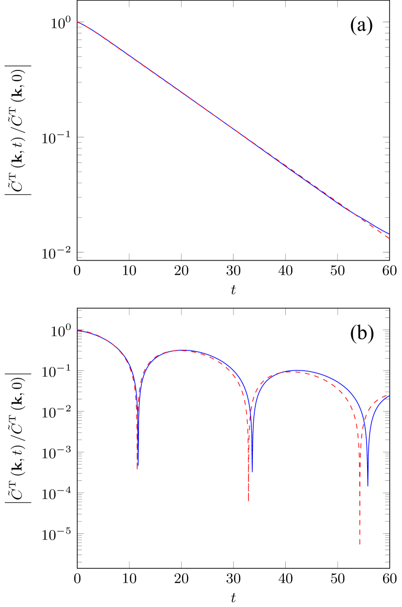
Figure 2: Transverse velocity autocorrelation functions of dumbbells, i.e., $N=2$, from simulations (solid) and analytical theory (dashed), Eqs. (32), (36), as a functions of time $t$ for the bond length (a) $l=1$ ($K=3$) and (b) $l=\sqrt{10}$ ($K=0.3$). The wave vector is in all cases $\bm{k}=(2\pi/30,0,0)^{T}$. As in Fig. 1, the correlation function in (b) assumes negative values (even loops). The theoretical curves are fitted to the simulation data.

VI.1.1 Dumbbell Fluid ($N=2$)

Results for the transverse velocity autocorrelation function of dumbbells of various bond lengths are displayed in Fig. 2. We like to mention that accurate simulation data for long times are rather demanding in terms of simulation time, both for viscous and viscoelastic fluids. The correlation functions typically decay over several orders of magnitude in the considered time range,Huang, Gompper, and Winkler (2012) and the MPC-intrinsic hydrodynamic fluctuations need to be averaged out. Nevertheless, good agreement is obtained between theory and simulations.

The qualitative different behavior in Fig. 2(a) and (b) is in agreement with the theoretical expectations discussed in Sec. IV.2, since the radicand in Eq. (35) is positive for $l=1$ and negative for $l=\sqrt{3}$. Hence, for $l=1$, the correlation function decays exponentially according to Eq. (36), whereas oscillations occur for longer bonds corresponding to Eq. (32). By fitting the theoretical expressions (32) and (36), respectively, we find the relaxation time $\tau_{1}\approx 2.8\,l^{2}$ (see also Ref. Kowalik and Winkler, 2013). This value agrees reasonably well with the theoretical prediction $3.1\,l^{2}$ following from the relaxation time Eq. (9) with the friction coefficient $\gamma=6\pi\eta R_{H}$, where the hydrodynamic radius of a monomer is $R_{H}=0.113$.Kowalik and Winkler (2013)

Evidently, our simulations and the theoretical approach yield long-range hydrodynamic correlations. The emergence of such correlations is not unexpected, since both the MPC simulations and the (generalized) Navier-Stokes equations conserve momentum. For the relatively short polymer chains, Rouse-like relaxation can be expected, because Zimm-type hydrodynamics requires long polymers, while the dumbbell relaxation time is only weakly affected by “fluid” correlations.Kowalik and Winkler (2013)

VI.1.2 Decamer Fluid ($N=10$)

Figure 3 presents simulation and theoretical results of $\tilde{C}^{T}(\bm{k},t)$ for decamers of various bond lengths. Fitting of Eq. (64) to the simulations data yields the relation $\tau_{1}\approx 54\,l^{2}$ for the bond-length dependence of the longest relaxation time. The theoretically predicted value $\tau_{1}\approx 63\,l^{2}$, according to Eq. (9), is somewhat larger, when the hydrodynamic radius $R_{H}=0.113$ is used.Kowalik and Winkler (2013) The relaxation times are, compared to a dumbbell fluid, longer and only damped oscillating correlation functions occur for the considered $\bm{k}$ vectors, as expected theoretically. The comparison of Fig. 3(a) and (b) indicates an increase in the frequency with increasing relaxation time, in agreement with the theoretical expectations. Moreover, the evident different time intervals between zeros of $\tilde{C}^{T}(\bm{k},t)$ in Fig. 3(b) reflect the presence of multiple relaxation times.

As for the dumbbell fluid, we find very good agreement between the simulation data and the theoretical prediction over the presented time window. In general, our results emphasize the strongly correlated polymer dynamics by the momentum-conserving interaction, i.e., long-range hydrodynamics.

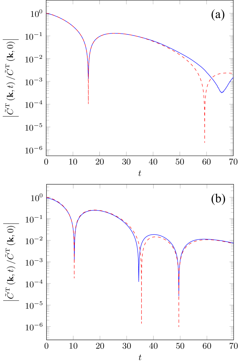
Figure 3: Transverse velocity autocorrelation functions of decameres ($N=10$) as a function of time $t$ from simulations (solid) and analytical theory (dashed) for the bond length (a) $l=1$ ($K=3$) and (b) $l=\sqrt{3}$ ($K=1$). The wave vector is $\bm{k}=(2\pi/30,0,0)^{T}$. As in Fig. 1, the correlation functions assume negative values (even loops). The theoretical curves are fitted to the simulation data.

VI.2 Center-of-Mass Velocity Correlation Function in Real Space

The autocorrelation function of the center-of-mass velocity of a polymer in real space, Eq. (V.1), can directly be calculated. For a compressible fluid, like the MPC fluid, $C_{cm}(t)$ comprises contributions from transverse and longitudinal modes, which cannot simply by extracted from the correlation function (V.1) determined in simulations. However, the longitudinal modes affect the short-time behavior of $C_{cm}(t)$ only, since the longitudinal correlation function decays exponentially,Huang, Gompper, and Winkler (2012, 2013) and the longer-time hydrodynamic properties are determined by the transverse correlation function with its long-time tail. Hence, the correlation function $C_{cm}(t)$ of the MPC fluid exhibits the correct long-time behavior. Moreover, the short-time behavior of the correlation function reflects the partitioning of space into collision cells of the MPC approach. Hydrodynamics appears only on length scales larger than the lattice constant $a$ of the collision-cell lattice.Huang, Gompper, and Winkler (2012) Consequently, at short times, $t\lesssim 5$ (Fig. 4), the simulation results deviate from the solution of the continuum Navier-Stokes equations, independent of polymer length, as is illustrated in Refs. Huang, Gompper, and Winkler, 2012, 2013; Poblete et al., 2014 for various systems. Therefore, agreement between theory and simulations can only be expected at longer times. This does not affect the dynamics of embedded colloids or polymers, because it is determined by the hydrodynamic long-time tail.

The correlation function for polymers of length $N=100$ and bond length $l=1$ is presented in Fig. 4. At $t=0$, $C_{\textrm{cm}}(0)=3k_{B}T/mN$ according to the equipartition theorem. (Note that this value includes transverse and longitudinal contributions.) For short times, i.e., for $t\lesssim 1$, $C_{\textrm{cm}}(t)$ reflects the discrete-time MPC procedure, with the first MPC collision at $t=h=0.1$. For $t\gtrsim 3$, the correlation function becomes negative due to viscoelasticity, as discussed in Sec. V.1.2, Eq. (55). At longer times, the correlation function decays in a power-law manner as $|C_{\textrm{cm}}(t)|\sim t^{-3/2}$, in agreement with the theoretical expectation for the regime $\tau_{l}\approx 1\ll t\ll\tau_{R}\approx 6\times 10^{3}$ (cf. Sec. V.1). In the simulations, we did not reach the asymptotic value for $t\to\infty$ (Eq. (46)), where the correlation function is positive again. The dependence $t^{-3/2}$ of the correlation function emphasizes and reflects the relevance of hydrodynamic interactions in a viscoelastic fluid of phantom polymers.

Figure 4: Time dependence of the velocity autocorrelation function for polymers with $N=100$ monomers and $l=1$ ($K=3$). The size of the simulation box is $L_{S}=100$. The dashed line indicates the power law $t^{-3/2}$.

VII Conclusions

We have presented a polymer-based model for a viscoelastic fluid and its implementation in a multiparticle collision dynamics algorithm. The fluid properties have been characterized by the transverse velocity autocorrelation function. The comparison between analytical predictions, based on the Navier-Stoks equation, and simulation results shows good agreement and, thus, confirms the suitability of applied implementation to describe viscoelastic fluids.

Polymer elasticity strongly affects the velocity correlation function $\tilde{C}^{T}(\bm{k},t)$, and leads to damped oscillations over a certain range of wave vectors. However, for long times and large length scales ($|\bm{k}|\to 0$), we expect and predict an exponential decay of $\tilde{C}^{T}(\bm{k},t)\sim e^{-\nu_{f}\bm{k}^{2}t}$ as function of time, with the kinematic viscosity of the polymeric fluid. This implies a long-time tail for the polymer center-of-mass velocity correlation function $C_{\textrm{cm}}(t)\sim t^{-3/2}$. On these scales, the polymer melt behaves as a fluid in terms of the correlation functions and, hence, exhibits hydrodynamics with the effective viscosity $\eta_{f}$. More interestingly, for very long polymers an additional power-law time regime can be identified. In the range $\tau_{l}<t<\tau_{R}$ between the relaxation time on the scale of a bond and the Rouse time of the whole polymer, with a nearly continuous mode spectrum, $\tilde{C}^{T}(\bm{k},t)$ is negative and exhibits the power-law dependence $t^{-3/2}$ rather than an exponential decay with time. Fourier transformation of the correlation function weighted by static structure factor maintains the time dependence, such that the polymer center-of-mass correlation function in real space shows the same time dependence. This rather distinct behavior is a consequence of the wide spectrum of modes, and thus, is a polymer-specific property. It reflects a strong influence of the polymer internal dynamics on the overall hydrodynamic behavior of the fluid.Huang, Gompper, and Winkler (2013)

Here, we have only considered phantom polymers. Extension to polymers with excluded-volume interactions would be interesting, specifically regarding the impact of excluded-volume interactions on the correlation functions. Yet, the results of Ref. Farago et al., 2012 show that even then the correlation function of a non-entangled polymer melt exhibits a long-time tail with the decay $t^{-3/2}$ in three dimensions.

Our results on the presence of a hydrodynamic long-time tail are consistent with theoretical predictions for phantom polymers. Freed and Perico (1981) However, as pointed out in Ref. Farago et al., 2012, the studies of self-avoiding polymers seem to contradict the widely accepted view that hydrodynamic interactions are screened in polymer melts. Doi and Edwards (1986) To be precise, the statement is typically used in the context of polymer solutions, where polymers are dissolved in a fluid, and momentum conservation is assumed to be violated for the fluid due to the immobile polymer matrix. Studies of the dynamical interplay of polymers and fluid would be desirable for a better understanding of screening. The presented simulation approach of polymers and fluid are very well suited for such an endeavor.

Appendix A General Inverse Laplace Transform of $\hat{C}^{T}(\bm{k},s)$

To calculate the inverse Laplace transform $\tilde{C}^{T}(\bm{k},t)$ of $\hat{C}^{T}(\bm{k},s)$ of Eq. (IV), the denominator of the right-hand side,

$$D(s)=\varrho s+\bm{k}^{2}\left(\eta+\varphi k_{B}T\sum_{p=1}^{N-1}\left(s+2/\tau_{n}\right)^{-1}\right),$$ (59)

is multiplied by $W(s)=\prod_{p=1}^{N-1}(s+2/\tau_{n})$, which yields

$$P(s)= \ D(s)W(s)$$ (60)

$$= \ (\varrho s+\eta\bm{k}^{2})W(s)+\bm{k}^{2}\varphi k_{B}T\sum_{n=1}^{N-1}\prod_{\begin{subarray}{c}p=1\\ p\neq n\end{subarray}}^{N-1}(s+2/\tau_{n}),$$

a polynomial in $s$ of degree $(N-1)$. Let $P_{n}$, $n=1,\ldots,M$, be the $M$ distinct roots of $\varrho^{-1}P\left(s\right)$, each of multiplicity $M_{n}$, so that $\sum_{n=1}^{M}M_{n}=N$, hence, $P(s)=\varrho\prod_{m=1}^{M}\left(s-P_{m}\right)^{M_{m}}$. For $W\!\left(s\right)$, which is also a polynomial in $s$, let $W_{n}$ be the coefficient of $s^{n}$, so that $W(s)=\sum_{m=0}^{N-1}W_{n}s^{n}$. Then, Section IV can be written as

$$\hat{C}^{T}(\bm{k},s) \ =\varrho\tilde{C}^{T}(\bm{k},0)\frac{W(s)}{P(s)}$$

$$\ =\tilde{C}^{T}(\bm{k},0)\sum_{n=0}^{N-1}\frac{W_{n}s^{n}}{\prod_{m=1}^{M}\left(s-P_{m}\right)^{M_{m}}}.$$ (61)

Inverse Laplace transformation of the terms ${s^{n}\prod_{m=1}^{M}(s-P_{m})^{-M_{m}}}$ yields Erdélyi et al. (1954); Prudnikov, Brychkov, and Marichev (1992)

$$\frac{\tilde{C}^{T}(\bm{k},t)}{\tilde{C}^{T}(\bm{k},0)}=\sum_{n=0}^{N-1}W_{n}\sum_{m=1}^{M}e^{P_{m}t}\sum_{l=1}^{M_{m}}\frac{A_{nml}(P_{m})t^{M_{m}-l}}{(M_{m}-l)!(l-1)!},$$ (62)

with

$$A_{nml}(x)=\frac{d^{l-1}}{dx^{l-1}}\left(x^{n}\prod_{\begin{subarray}{c}j=1\\ j\neq m\end{subarray}}^{M}\left(x-P_{j}\right)^{-M_{j}}\right).$$ (63)

Note that the degree of the polynomial of the enumerator is higher than the one of the denominator. If $P\!\left(s\right)$ only has simple roots, i.e., $M_{n}=1$ for all $n$, Eq. (62) simplifies to Oberhettinger and Badii (2012); Erdélyi et al. (1954)

$$\frac{\tilde{C}^{T}(\bm{k},t)}{\tilde{C}^{T}(\bm{k},0)}=\sum_{n=0}^{N-1}W_{n}\sum_{m=1}^{N}P_{m}^{n}e^{P_{m}t}\prod_{\begin{subarray}{c}j=1\\ j\neq m\end{subarray}}^{N}\left(P_{m}-P_{j}\right)^{-1}.$$ (64)

Appendix B Inverse Laplace Transformation for Continuous Polymer

The correlation function (42) is of the form

$$\hat{f}(s)=\frac{1}{s+b/\sqrt{s}}=\frac{\sqrt{s}}{s^{3/2}+b}.$$ (65)

The inverse Laplace-transform $f(t)={\cal{L}}^{-1}[\hat{f}(s);t]$ can be obtained from that of $\hat{H}(\sqrt{s})$, defined as

$$\hat{H}(s)=\frac{s}{s^{3}+b},$$ (66)

according to Oberhettinger and Badii (2012)

$$f(t)= \ {\cal{L}}^{-1}[\hat{f}(s);t]={\cal{L}}^{-1}[\hat{H}(\sqrt{s});t]$$

$$= \ \frac{1}{2\sqrt{\pi t^{3}}}\int_{0}^{\infty}\tau\operatorname{exp}\left(-\frac{\tau^{2}}{4t}\right)H(\tau)d\tau.$$ (67)

Partial fraction decomposition of $s^{3}+b$ in $\hat{H}(\sqrt{s})$ and straightforward inverse Laplace transformation yields

$$H(t)=\frac{1}{3\sqrt[3]{b}}\left(e^{\kappa t}\operatorname{cos}(\omega t)+\sqrt{3}e^{\kappa t}\operatorname{sin}(\omega t)-e^{-2\kappa t}\right),$$ (68)

with the abbreviations $\kappa=\sqrt[3]{b}/2$ and $\omega=\sqrt{3}\sqrt[3]{b}/2$. Evaluation of the integral (67) gives, with (68),

$$f(x)=\frac{1}{3} \left\{\mathrm{erfcx}\left(-\frac{1}{2}[1+i\sqrt{3}]\sqrt{x}\right)\right.$$

$$\left.+\ \mathrm{erfcx}\left(-\frac{1}{2}[1-i\sqrt{3}]\sqrt{x}\right)+\ \mathrm{erfcx}\left(\sqrt{x}\right)\right\},$$ (69)

with $x=b^{2/3}t$. Here, $\mathrm{erfcx}(y)$ is the scaled complementary error function

$$\mathrm{erfcx}(y)=e^{y^{2}}\left(1-\frac{2}{\sqrt{\pi}}\int_{0}^{y}e^{-u^{2}}du\right).$$ (70)

We like to mention that Laplace transformation of Eq. (42) including $\eta$ can be performed in a similar manner.

Appendix C Center-of-Mass Velocity Autocorrelation Function—Connection to Dynamic Structure Factor

The polymer center-of-mass correlation function is given by (cf. Eq. (V.1))

$$C_{\textrm{cm}}(t)=\frac{1}{N^{2}}\sum_{i=1}^{N}\sum_{j=1}^{N}\left\langle\bm{v}(\bm{r}_{i},t)\cdot\bm{v}(\bm{r}_{j},0)\right\rangle.$$ (71)

The Fourier representation

$$\bm{v}(\bm{r}_{i},t)=\frac{1}{(2\pi)^{2}}\int\tilde{\bm{v}}(\bm{k},t)e^{i\bm{k}\cdot\bm{r}_{i}(t)}d^{3}k$$ (72)

yields

$$C_{\textrm{cm}}(t)=\frac{1}{N^{2}(2\pi)^{2}}$$ (73)

$$\times\sum_{i=1}^{N}\sum_{j=1}^{N}\left\langle\tilde{\bm{v}}(\bm{k},t)\cdot\tilde{\bm{v}}(\bm{k}^{\prime},0)\right\rangle e^{i\bm{k}\cdot\bm{r}_{i}(t)}e^{i\bm{k}^{\prime}\cdot\bm{r}_{j}(0)}d^{3}kd^{3}k^{\prime}.$$

With the definition of the fluid correlation function $\langle\tilde{\bm{v}}(\bm{k},t)\cdot\tilde{\bm{v}}(\bm{k}^{\prime},0)\rangle\sim\delta(\bm{k}+\bm{k}^{\prime})\tilde{C}(\bm{k},t)$ (IV), and the dynamic structure factor (V.1)

$$S(\bm{k},t)=\frac{1}{N}\sum_{i=1}^{N}\sum_{j=1}^{N}\langle e^{i\bm{k}\cdot(\bm{r}_{i}(t)-\bm{r}_{j}(0))}\rangle,$$ (74)

Eq. (71) becomes

$$C_{\textrm{cm}}^{T}(t)=\frac{1}{(2\pi)^{3}N}\int S(\bm{k},t){\tilde{C}}^{T}(\bm{k},t)d^{3}k,$$ (75)

which is Eq. (51).

References

- Dhont et al. (2008) J. K. G. Dhont, G. Gompper, G. Nägele, D. Richter, and R. G. Winkler, eds., Soft Matter: From Synthetic to Biological Materials, Lecture notes of the 39th IFF Spring School (Forschungzentrum Jülich, Jülich, 2008).
- Menzel (2015) A. M. Menzel, “Tuned, driven, and active soft matter,” Physics Reports 554, 1 (2015).
- Nagel (2017) S. R. Nagel, “Experimental soft-matter science,” Rev. Mod. Phys. 89, 025002 (2017).
- Ellis (2001) R. J. Ellis, “Macromolecular crowding: an important but neglected aspect of the intracellular environment,” Curr. Opin. Struct. Biol. 11, 114 (2001).
- Bucciarelli et al. (2016) S. Bucciarelli, J. S. Myung, B. Farago, S. Das, G. A. Vliegenthart, O. Holderer, R. G. Winkler, P. Schurtenberger, G. Gompper, and A. Stradner, “Dramatic influence of patchy attractions on short-time protein diffusion under crowded conditions,” Sci. Adv. 2, e1601432 (2016).
- Bird, Armstrong, and Hassager (1987) R. B. Bird, R. C. Armstrong, and O. Hassager, Dynamics of Polymer Liquids, Vol. 1 (John Wiley & Sons, New York, 1987).
- Dhont (1996) J. K. G. Dhont, An Introduction to Dynamics of Colloids (Elsevier, Amsterdam, 1996).
- Ferry (1980) J. D. Ferry, Viscoelastic Properties of Polymers (Wiley, New York, 1980).
- Bird et al. (1987) R. B. Bird, C. F. Curtiss, R. C. Armstrong, and O. Hassager, Dynamics of Polymer Liquids, Vol. 2 (John Wiley & Sons, New York, 1987).
- Doi and Edwards (1986) M. Doi and S. F. Edwards, The Theory of Polymer Dynamics (Clarendon Press, Oxford, 1986).
- Larson (1999) R. G. Larson, The Structure and Rheology of Complex Fluids (Oxford University, New York, 1999).
- Winkler, Fedosov, and Gompper (2014) R. G. Winkler, D. A. Fedosov, and G. Gompper, “Dynamical and rheological properties of soft colloid suspensions,” Curr. Opin. Colloid Interface Sci. 19, 594 (2014).
- Tao, Götze, and Gompper (2008) Y.-G. Tao, I. O. Götze, and G. Gompper, “Multiparticle collision dynamics modeling of viscoelastic fluids,” J. Chem. Phys. 128, 144902 (2008).
- Kowalik and Winkler (2013) B. Kowalik and R. G. Winkler, “Multiparticle collision dynamics simulations of viscoelastic fluids: Shear-thinning Gaussian dumbbells,” J. Chem. Phys. 138, 104903 (2013).
- McNamara and Zanetti (1988) G. R. McNamara and G. Zanetti, “Use of the Boltzmann equation to simulate lattice-gas automata,” Phys. Rev. Lett. 61, 2332 (1988).
- Shan and Chen (1993) X. Shan and H. Chen, “Lattice Boltzmann model for simulating flows with multiple phases and components,” Phys. Rev. E 47, 1815 (1993).
- Succi (2001) S. Succi, The lattice Boltzmann equation: for fluid dynamics and beyond (Oxford University Press, 2001).
- Dünweg and Ladd (2009) B. Dünweg and A. C. Ladd, “Lattice Boltzmann simulations of soft matter systems,” Adv. Polym. Sci. 221, 89 (2009).
- Hoogerbrugge and Koelman (1992) P. J. Hoogerbrugge and J. M. V. A. Koelman, “Simulating microscopic hydrodynamics phenomena with dissipative particle dynamics,” Europhys. Lett. 19, 155 (1992).
- Español and Warren (1995) P. Español and P. B. Warren, “Statistical mechanics of dissipative particle dynamics,” Europhys. Lett. 30, 191 (1995).
- Malevanets and Kapral (1999) A. Malevanets and R. Kapral, “Mesoscopic model for solvent dynamics,” J. Chem. Phys. 110, 8605 (1999).
- Kapral (2008) R. Kapral, “Multiparticle collision dynamics: Simulations of complex systems on mesoscale,” Adv. Chem. Phys. 140, 89 (2008).
- Gompper et al. (2009) G. Gompper, T. Ihle, D. M. Kroll, and R. G. Winkler, “Multi-particle collision dynamics: A particle-based mesoscale simulation approach to the hydrodynamics of complex fluids,” Adv. Polym. Sci. 221, 1 (2009).
- Ispolatov and Grant (2002) I. Ispolatov and M. Grant, “Lattice boltzmann method for viscoelastic fluids,” Phys. Rev. E 65, 056704 (2002).
- Dellar (2014) P. Dellar, “Lattice Boltzmann formulation for linear viscoelastic fluids using an abstract second stress,” SIAM J. Sci. Comput. 36, A2507 (2014).
- Fedosov et al. (2011) D. A. Fedosov, W. Pan, B. Caswell, G. Gompper, and G. E. Karniadakis, “Predicting human blood viscosity in silico,” Proc. Natl. Acad. Sci. USA 108, 11772 (2011).
- Fedosov et al. (2012) D. A. Fedosov, S. P. Singh, A. Chatterji, R. G. Winkler, and G. Gompper, “Semidilute solutions of ultra-soft colloids under shear flow,” Soft Matter 8, 4109 (2012).
- Huang et al. (2010a) C.-C. Huang, R. G. Winkler, G. Sutmann, and G. Gompper, “Semidilute polymer solutions at equilibrium and under shear flow,” Macromolecules 43, 10107 (2010a).
- Nikoubashman and Likos (2010a) A. Nikoubashman and C. N. Likos, “Branched polymers under shear,” Macromolecules 43, 1610 (2010a).
- Singh et al. (2013) S. P. Singh, A. Chatterji, G. Gompper, and R. G. Winkler, “Dynamical and rheological properties of ultrasoft colloids under shear flow,” Macromolecules 46, 8026 (2013).
- Winkler et al. (2013) R. G. Winkler, S. P. Singh, C.-C. Huang, D. A. Fedosov, K. Mussawisade, A. Chatterji, M. Ripoll, and G. Gompper, “Mesoscale hydrodynamics simulations of particle suspensions under shear flow: From hard to ultrasoft colloids,” Eur. Phys. J. Spec. Top. 222, 2773 (2013).
- Toneian (2019) D. Toneian, Magnetically Functionalized Star Polymers and Polymer Melts in MPCD Simulations, Ph.D. thesis, TU Wien (2019).
- Toneian, Likos, and Kahl (2019) D. Toneian, C. N. Likos, and G. Kahl, “Controlled self-aggregation of polymer-based nanoparticles employing shear flow and magnetic fields,” J. Phys: Condens. Matter 31, 24LT02 (2019), arXiv:1904.01535 [cond-mat.soft] .
- Noguchi and Gompper (2004) H. Noguchi and G. Gompper, “Fluid vesicles with viscous membranes in shear flow,” Phys. Rev. Lett. 93, 258102 (2004).
- Somfai, Morozov, and van Saarloos (2006) E. Somfai, A. Morozov, and W. van Saarloos, “Modeling viscoelastic flow with discrete methods,” Physica A 362, 93 (2006).
- Fedosov, Karniadakis, and Caswell (2010) D. A. Fedosov, G. E. Karniadakis, and B. Caswell, “Steady shear rheometry of dissipative particle dynamics models of polymer fluids in reverse Poiseuille flow,” J. Chem. Phys. 132, 144103 (2010).
- Ji et al. (2011) S. Ji, R. Jiang, R. G. Winkler, and G. Gompper, “Mesoscale hydrodynamic modeling of a colloid in shear-thinning viscoelastic fluids under shear flow,” J. Chem. Phys. 135, 134116 (2011).
- Toneian (2015) D. Toneian, Multi-Particle Collision Dynamics Simulation of Viscoelastic Fluids, Master’s thesis, TU Wien (2015).
- de Gennes (1979) P.-G. de Gennes, Scaling Concepts in Polymer Physics (Cornell University, Ithaca, 1979).
- Freed and Perico (1981) K. F. Freed and A. Perico, “Considerations on the multiple scattering representation of the concentration dependence of the viscoelastic properties of polymer systems,” Macromolecules 14, 1290 (1981).
- Farago, Meyer, and Semenov (2011) J. Farago, H. Meyer, and A. N. Semenov, “Anomalous diffusion of a polymer chain in an unentangled melt,” Phys. Rev. Lett. 107, 178301 (2011).
- Farago et al. (2012) J. Farago, H. Meyer, J. Baschnagel, and A. N. Semenov, “Mode-coupling approach to polymer diffusion in an unentangled melt. ii. the effect of viscoelastic hydrodynamic interactions,” Phys. Rev. E 85, 051807 (2012).
- Mussawisade et al. (2005) K. Mussawisade, M. Ripoll, R. G. Winkler, and G. Gompper, “Dynamics of polymers in a particle based mesoscopic solvent,” J. Chem. Phys. 123, 144905 (2005).
- Ryder and Yeomans (2006) J. F. Ryder and J. M. Yeomans, “Shear thinning in dilute polymer solutions,” J. Chem. Phys. 125, 194906 (2006).
- Frank and Winkler (2008) S. Frank and R. G. Winkler, “Polyelectrolyte electrophoresis: Field effects and hydrodynamic interactions,” EPL 83, 38004 (2008).
- Chelakkot, Winkler, and Gompper (2012) R. Chelakkot, R. G. Winkler, and G. Gompper, “Flow-induced helical coiling of semiflexible polymers in structured microchannels,” Phys. Rev. Lett. 109, 178101 (2012).
- Nikoubashman and Likos (2010b) A. Nikoubashman and C. N. Likos, “Flow-induced polymer translocation through narrow and patterned channels,” J. Chem. Phys. 133, 074901 (2010b).
- Huang, Gompper, and Winkler (2013) C. C. Huang, G. Gompper, and R. G. Winkler, “Effect of hydrodynamic correlations on the dynamics of polymers in dilute solution,” J. Chem. Phys. 138, 144902 (2013).
- Ripoll, Winkler, and Gompper (2006) M. Ripoll, R. G. Winkler, and G. Gompper, “Star polymers in shear flow,” Phys. Rev. Lett. 96, 188302 (2006).
- Singh et al. (2014) S. P. Singh, C.-C. Huang, E. Westphal, G. Gompper, and R. G. Winkler, “Hydrodynamic correlations and diffusion coefficient of star polymers in solution,” J. Chem. Phys. 141, 084901 (2014).
- Ghavami and Winkler (2017) A. Ghavami and R. G. Winkler, “Solvent induced inversion of core–shell microgels,” ACS Macro Lett. 6, 721 (2017).
- Westphal et al. (2014) E. Westphal, S. P. Singh, C.-C. Huang, G. Gompper, and R. G. Winkler, “Multiparticle collision dynamics: GPU accelerated particle-based mesoscale hydrodynamic simulations,” Comput. Phys. Comm. 185, 495 (2014).
- Howard, Panagiotopoulos, and Nikoubashman (2018) M. P. Howard, A. Z. Panagiotopoulos, and A. Nikoubashman, “Efficient mesoscale hydrodynamics: Multiparticle collision dynamics with massively parallel GPU acceleration,” Comput. Phys. Commun. 230, 10 (2018).
- Felderhof (2005) B. U. Felderhof, “Backtracking of a sphere slowing down in a viscous compressible fluid,” J. Chem. Phys. 123, 044902 (2005).
- Alder and Wainwright (1970) B. J. Alder and T. E. Wainwright, “Decay of the Velocity Autocorrelation Function,” Phys. Rev. A 1, 18 (1970).
- Zwanzig and Bixon (1970) R. Zwanzig and M. Bixon, “Hydrodynamic theory of the velocity correlation function,” Phys. Rev. A 2, 2005 (1970).
- Ernst, Hauge, and van Leeuwen (1971) M. H. Ernst, E. H. Hauge, and J. M. J. van Leeuwen, “Asymptotic time behavior of correlation functions. i. kinetic terms,” Phys. Rev. A 4, 2055 (1971).
- Hauge and Martin-Löf (1973) E. Hauge and A. Martin-Löf, “Fluctuating hydrodynamics and Brownian motion,” J. Stat. Phys. 7, 259 (1973).
- Hinch (1975) E. J. Hinch, “Application of the langevin equation to fluid suspensions,” J. Fluid Mech. 72, 499 (1975).
- Huang, Gompper, and Winkler (2012) C.-C. Huang, G. Gompper, and R. G. Winkler, “Hydrodynamic correlations in multiparticle collision dynamics fluids,” Phys. Rev. E 86, 056711 (2012).
- Winkler and Reineker (1992) R. G. Winkler and P. Reineker, “Finite size distribution and partition functions of Gaussian chains: Maximum entropy approach,” Macromolecules 25, 6891 (1992).
- Harnau, Winkler, and Reineker (1997) L. Harnau, R. G. Winkler, and P. Reineker, “Influence of stiffness on the dynamics of macromolecules in a melt,” J. Chem. Phys. 106, 2469 (1997).
- Verdier (1966) P. H. Verdier, “Monte Carlo studies of lattice-model polymer chains. I. correlation functions in the statistical-bead model,” J. Chem. Phys. 45, 2118 (1966).
- Kopf, Dünweg, and Paul (1997) A. Kopf, B. Dünweg, and W. Paul, “Dynamics of polymer “isotope” mixtures: Molecular dynamics simulation and Rouse model analysis,” J. Chem. Phys. 107, 6945 (1997).
- Winkler (1999) R. G. Winkler, “Analytical calculation of the relaxation dynamics of partially stretched flexible chain molecules: Necessity of a wormlike chain description,” Phys. Rev. Lett. 82, 1843 (1999).
- Winkler (2010) R. G. Winkler, “Conformational and rheological properties of semiflexible polymers in shear flow,” J. Chem. Phys. 133, 164905 (2010).
- Landau and Lifshitz (1959) L. D. Landau and E. M. Lifshitz, Fluid Mechanics (Pergamon Press, London, 1959).
- Frenkel and Smit (2002) D. Frenkel and B. Smit, Understanding Molecular Simulation, 2nd ed. (Academic Press, 2002).
- Ihle and Kroll (2001) T. Ihle and D. M. Kroll, “Stochastic rotation dynamics: A Galilean-invariant mesoscopic model for fluid flow,” Phys. Rev. E 63, 020201(R) (2001).
- Ripoll et al. (2005) M. Ripoll, K. Mussawisade, R. G. Winkler, and G. Gompper, “Dynamic regimes of fluids simulated by multi-particle-collision dynamics,” Phys. Rev. E 72, 016701 (2005).
- Tüzel, Ihle, and Kroll (2006) E. Tüzel, T. Ihle, and D. M. Kroll, “Dynamic correlations in stochastic rotation dynamics,” Phys. Rev. E 74, 056702 (2006).
- Huang et al. (2010b) C. Huang, A. Chatterji, G. Sutmann, G. Gompper, and R. G. Winkler, “Cell-level canonical sampling by velocity scaling for multiparticle collision dynamics simulations,” J. Comput. Phys. 229, 168–177 (2010b).
- (73) D. Toneian, OpenMPCD.
- Malevanets and Kapral (2000) A. Malevanets and R. Kapral, “Solute molecular dynamics in a mesoscale solvent,” J. Chem. Phys. 112, 7260 (2000).
- CUD (2015) CUDA C Programming Guide, Version 7.5, NVIDIA (2015).
- Huang et al. (2015) C.-C. Huang, A. Varghese, G. Gompper, and R. G. Winkler, “Thermostat for nonequilibrium multiparticle-collision-dynamics simulations,” Phys. Rev. E 91, 013310 (2015).
- Dyke (2014) P. Dyke, An Introduction to Laplace Transforms and Fourier Series, 2nd ed., edited by M. A. J. Chaplain, K. Erdmann, A. MacIntyre, E. Süli, M. R. Tehranchi, and J. F. Toland, Springer Undergraduate Mathematics Series (Springer, 2014).
- Oberhettinger and Badii (2012) F. Oberhettinger and L. Badii, Tables of Laplace transforms (Springer Science & Business Media, 2012).
- Winkler, Keller, and Rädler (2006) R. G. Winkler, S. Keller, and J. O. Rädler, “Intramolecular dynamics of linear macromolecules by fluorescence correlation spectroscopy,” Phys. Rev. E 73, 041919 (2006).
- Harnau, Winkler, and Reineker (1996) L. Harnau, R. G. Winkler, and P. Reineker, “Dynamic structure factor of semiflexible macromolecules in dilute solution,” J. Chem. Phys. 104, 6355 (1996).
- Winkler, Harnau, and Reineker (1997) R. G. Winkler, L. Harnau, and P. Reineker, “Distribution functions and dynamical properties of stiff macromolecules,” Macromol. Theory Simul. 6, 1007 (1997).
- Poblete et al. (2014) S. Poblete, A. Wysocki, G. Gompper, and R. G. Winkler, “Hydrodynamics of discrete-particle models of spherical colloids: A multiparticle collision dynamics simulation study,” Phys. Rev. E 90, 033314 (2014).
- Erdélyi et al. (1954) A. Erdélyi, W. Magnus, F. Oberhettinger, and F. G. Tricomi, Tables of Integral Transforms, Vol. 1 (McGraw-Hill, New York, 1954).
- Prudnikov, Brychkov, and Marichev (1992) A. P. Prudnikov, Y. A. Brychkov, and O. I. Marichev, Integrals and Series, Vol. 5 (Gordon and Breach Science Publishers, 1992).