The gallium anomaly reassessed using a Bayesian approach

Abstract

The solar-neutrino detectors GALLEX Anselmann1995 ; Hampel1998 ; Kaether2010 and SAGE Abdurashitov were calibrated by electron-neutrino flux from the ³⁷Ar and ⁵¹Cr calibration sources. A deficit in the measured neutrino flux was recorded by counting the number of neutrino-induced conversions of the ⁷¹Ga nuclei to ⁷¹Ge nuclei. This deficit was coined “gallium anomaly” and it has lead to speculations about beyond-the-standard-model physics in the form of eV-mass sterile neutrinos. Notably, this anomaly has already defied final solution for more than 20 years. Here we reassess the statistical significance of this anomaly and improve the related statistical approaches by treating the neutrino experiments as repeated Bernoulli trials taking into account the fact that the number of the detected ⁷¹Ge nuclei is quite small, thus calling for a Bayesian statistical approach. In addition, we take into account the systematic errors of the experiments, their correlations, theoretical uncertainties and the number of background solar-neutrino events as a Poisson-distributed random variable. To compare with the previously reported statistical significances of the anomaly we convert the posterior intervals of our Bayesian approach to standard deviations $\sigma$ of the frequentist approach. We find that our approach reduces the statistical significance of the anomaly by $0.8\,\sigma$ for all the adopted theoretical approaches. This renders the gallium anomaly a statistically weakly supported concept. Furthermore, the implications of our approach go far beyond the gallium anomaly since the results of many rare-events experiments should be reassessed for their limited number of recorded events.

Main

The Gallium-based solar-neutrino detectors of the GALLEX Anselmann1995 ; Hampel1998 ; Kaether2010 and SAGE Abdurashitov experiments have been subjected to detection-efficiency testing with strong ³⁷Ar and ⁵¹Cr neutrino sources. The neutrinos emitted by these sources have discrete energies below 1 MeV. The detection is based on the charged-current neutrino-nucleus scattering reaction

$$\nu_{e}+\,^{71}{\rm Ga}(3/2^{-}_{\rm g.s.})\ \rightarrow\,^{71}{\rm Ge}(J^{\pi})+e^{-},$$ (1)

leading to low-lying states of multipolarity $J^{\pi}$ in ${}^{71}\rm Ge$, mainly to the ground state and the excited states at 175 keV and 500 keV.

The neutrino-nucleus scattering cross section for the scattering to the ground state can be deduced from the half-life of ⁷¹Ge and is thus well known Bahcall1997 . However, the total cross section contains also the scatterings to the excited states as well. Being short-lived states, the cross section for these states cannot be determined via $\beta$-decay half-life measurements, and so other methods must be employed. Two ways for dealing with this have been proposed: Use either charge-exchange reactions to probe the Gamow-Teller strength for transitions from the ground state of ${}^{71}\rm Ga$ to the states in ${}^{71}\rm Ge$ Frekers:2011zz or use a microscopic nuclear model, such as the nuclear shell model Haxton:1998uc ; Kostensalo2019 , to directly compute the cross sections for the scattering transitions to the ${}^{71}\rm Ge$ final states. With both of these approaches the theoretical estimates have been systematically larger than the values reported by GALLEX and SAGE, the experimental values being for example 0.87 $\pm$ 0.05 times the cross sections based on the theory estimates by Bahcall Bahcall1997 . The origins of these discrepancies have been previously discussed in Giunti2011 ; Haxton:1998uc ; Giunti:2012tn . The mismatch between the measured and theoretical cross sections constitutes the so-called “gallium anomaly”.

One of the suggested explanations for the anomaly is the oscillation of the electron neutrino to an eV mass-scale sterile neutrino Giunti2011 ; Giunti:2012tn , which could potentially also explain the so-called “reactor-antineutrino anomaly” Mueller2011 ; Mention:2011rk ; Huber:2011wv . However, it should be remarked here that there is no accepted sterile-neutrino model which could explain the experimental anomalies consistently. Less exotic solutions to the reactor-antineutrino anomaly, like the proper inclusion of first-forbidden $\beta$-decay branches in the construction of the cumulative antineutrino spectra, have also been suggested Hayen2019a ; Hayen2019b .

The GALLEX and SAGE experiments (gallium experiments for short) can be thought of as repeated Bernoulli trials with a single ⁷¹Ga atom in a small area (measured in cm²) with a projectile neutrino hitting the square in a uniformly distributed random spot. The result of one of these trials can be either a “success” (i.e. neutrino-nucleus scattering happens) or a “failure” (no scattering). The cross section (in cm²) is the probability of the scattering to occur. The experiments record the number of germanium atoms produced (from which one can deduce the number of events), the neutrino flux, and the number of target atoms to some finite accuracy, reporting the cross section as a (possibly asymmetric) normal distribution. In the papers Anselmann1995 ; Hampel1998 ; Kaether2010 ; Abdurashitov the statistical errors are related to the number of Bernoulli trials (neutrino flux, number of target nuclei) and successes (number of ⁷¹Ge atoms produced). While the normal-distribution approximation is asymptotically valid for large number of trials (and events), this condition is not well satisfied in the gallium experiments (or in any rare-events experiment with a small number of recorded events), since the number of observed events is small.

The small number of events recorded in the gallium experiments produces a major source of uncertainty in their reported results. The number of events in the experiments varied between approximately 360 and 520 Anselmann1995 ; Hampel1998 ; Kaether2010 ; Abdurashitov ; GallexPC . Basic probability theory tells us that given the number of successes $s$ and attempts $n$ in a repeated Bernoulli trial the success probability $p$ has a likelihood function ${\rm Beta}(s,n-s)$. The relative error (the ratio of the standard deviation to the expected value) for small success probabilities follows the law $1/\sqrt{s}$, and is thus valid for the neutrino experiments. This uncertainty is then 4.2–5.2 % in the gallium experiments. Moreover, the cross-section distribution is highly asymmetric for such small success probabilities. Since the relative uncertainty is not proportional to the number of trials but only depends on the number of successes, we can take the small area which the neutron hits to be 1 cm², since then the numerical value of the cross section is the probability of success in a single trial. Note that we could have equivalently picked an area e.g. 0.25 cm² with the number of trials being reduced to fourth and the parameter here being four times the cross section and the results would remain unchanged.

In the analysis of the GALLEX and SAGE experiments the production rate of ⁷¹Ge, that is, how many neutrinos interacted with the detector in a day, was assessed for the individual runs (3–28 days) separately. The analysis was based on a maximum likelihood fit with constant solar neutrino background. The final result was derived by taking an average weighted by the inverse variances of the individual runs. However, there is a much more simple way to deal with the solar-neutrino background and to combine the individual runs. Since we assume that the neutrino interactions are independent we can see that the events are exchangeable gelman_bda . This means that we do not get any more information by knowing the number of events in the individual runs. The total number of events is a sufficient statistic (see e.g. davison ) meaning that all the relevant information regarding the probability of success (cross section) is included in this number. Thus a more straight-forward way would be to measure the total number of events (including the background) and subtract the number of background events as a Poisson distributed variable. The resulting distribution can then by calculated by simulation.

In this paper we revisit the statistical significance of the gallium anomaly by reassessing the ratio $R$ between the cross sections of the GALLEX and SAGE experiments and those of the theory using a Bayesian approach. In this spirit we construct posterior distributions for $R$ and our simulation-based approach allows us to take into account properly such details as the correlations between the systematic errors of the two GALLEX experiments as well as between the two SAGE experiments.

Figure 1: Posterior distributions for the experiment-to-theory ratio $R$. The normal distributions are those used in the previous analyses of the gallium experiments.

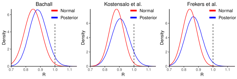
The difference between the simple normal distributions used in the recent survey Kostensalo2019 and the properly constructed posterior distributions for the ratio $R$ are shown in Fig. 1 for the estimates of Bahcall Bahcall1997 , the shell-model results of Kostensalo et al. Kostensalo2019 and the charge-exchange results of Frekers et al. Frekers:2011zz . As clearly visible from the figures, the posterior distributions are wider than the previously adopted normal distributions and they are shifted slightly to the right. In addition, the skewness of these distributions shifts probability to the right of $R=1$ relative to the normal distributions. Since the uncertainty related to estimating the success probability $p$ of a binomial distribution is proportional to the inverse square root of the number of successes, this error is larger in the experiments with lower number of successes. This means that for the normal distributions the experiments with a low number of events are overweighted relative to the rest of the experiments, making the anomaly appear larger than it actually is.

Theory	Posterior ETI	Significance ($\sigma$)	Normal Kostensalo2019 ($\sigma$)
Bachall	0.936	1.85	2.6
Bachall corr.	0.894	1.62
Kostensalo et al.	0.873	1.52	2.3
Frekers et al.	0.974	2.22	3.0
Frekers et al. corr.	0.942	1.90
Combined theory	0.915	1.72

Table 1: Magnitude of the gallium anomaly in different theoretical frameworks. The column “Posterior ETI” gives the width of the smallest equivalently-tailed posterior interval in which the experiment to theory ratio 1 is included. Column “Significance” gives the corresponding significance for a normal distribution in standard deviations $\sigma$. The last column gives the previously reported standard deviations, all distributions being assumed to be normal and the systematic errors independent, even for the same detectors. The second and fifth rows include a 30% tensor correction for the excited states. The “Combined theory” in the last row includes the tensor-corrected Bachall, Kostensalo et al., and the tensor-corrected Frekers el al. results weighted by their inverse variances.

The statistical significances of the results are given in Table 1. The results are reported as equivalent-tailed posterior intervals (ETI), that is, the null-hypothesis (no anomaly) is included, for example, in the 93.6% posterior interval of the uncorrected Bahcall results. To allow a simple comparison with the previously reported results, this is also expressed in a frequentistic way as sigmas of a normal-distribution (the column “Significance”). The drop in the corresponding frequentistic significance is about 0.8 $\sigma$ for all the theoretical models. The most recent theoretical estimate by Kostensalo et al. gives no evidence in favor of the gallium anomaly. Furthermore, the combined theoretical results also includes $R=1$ in the 95% ETI. Without any tensor corrections the Frekers et al. results still noticeably deviate from the GALLEX and SAGE results but only at 2.22 $\sigma$ instead of the previously reported 3.0 $\sigma$. Tensor contributions of the magnitude proposed in Kostensalo2019 seem to be able to explain away most of the remaining discrepancies.

In this Letter the statistical significance of the so-called “gallium anomaly” was reassessed using a Bayesian approach, in which we constructed posterior probability distributions for the ratio $R$ of the experimental and theoretical cross sections. It was pointed out that a neutrino-detection experiment can be formulated as a repeated Bernoulli trial with the reported cross section being the probability of “success” i.e. a detected event. This means, that even with perfect knowledge of the number of detected events, neutrinos hitting the target, and number of target nuclei, one would end up with a beta distribution for the cross section. This conclusion goes even beyond the present context and embraces all rear-events experiments with a limited number of detected events.

The size of the gallium anomaly was assessed by a simulation taking into account the systematic and statistical errors in the GALLEX and SAGE experiments, theoretical uncertainties, correlations in systematic errors, the number of the background solar-neutrino events as a Poisson distributed random variable, as well as the relatively small number of neutrinos observed. The recent shell-model results of Kostensalo et al. were shown to agree with the GALLEX and SAGE results within the 95 % posterior interval. In a previous frequentistic analysis Giunti2011 , this significance was reported as 2.3 $\sigma$. Taking into account all the theoretical estimates with proper corrections for tensor contributions, the theoretical and experimental results are shown to agree within the 95 % posterior interval. This means that there is little evidence of the gallium anomaly relating to new physics.

Methods

We adopt a Bayesian approach gelman_bda to reassess the significance of the discrepancies between the theoretical cross sections and the results from GALLEX and SAGE gallium experiments. We construct posterior distributions for the ⁵¹Cr and ³⁷Ar cross sections from which we obtain a posterior distribution for the theory-to-experiment ratio $R$. The approach is motivated by a multitude of reasons: First, we can easily incorporate various heterogeneous sources of uncertainty in the statistical model, including the correlated systematic errors of the two GALLEX experiments, without having to resort to approximations. Second, while the models for the true number of unobserved events, the total number of neutrinos and the cross sections are fairly simple, the hierarchical structure quickly becomes more complicated when we connect the actual measured quantities to the true underlying latent variables, making a graphical model suitable for the task. Third, powerful computational methods are readily available for Markov chain Monte Carlo (MCMC) simulations.

Table 2: The number of events (neutrino-nucleus interactions) and the number of Bernoulli trials in each gallium experiment based on all the available information. A single trial consists of one neutrino hitting a 1 cm² square with a single gallium atom in a uniformly distributed random spot. To avoid underestimating the thickness of the tails we avoid approximating e.g. the product of normal distributions as a normal distribution. The reports of SAGE included more details in regard to the experimental set-up, which is why the expression for the number of trials differs from GALLEX. While the normal approximation would work fine here we want to stress that this is not true in general.

	Method	Trials ($10^{44}$)	Events
GALLEX 1	51Cr	$703.9^{+12.21}_{-17.76}$(stat.) ${}^{+3.520}_{-3.942}$(syst.)	$389.76\pm 38.28$
GALLEX 2	51Cr	$775.6^{+37.04}_{-17.76}$(stat.) ${}^{+3.878}_{-4.343}$(syst.)	$365.93\pm 41.82$
SAGE 1	51Cr	$6.766\times(72.6\pm 0.2)\times(1.9114\pm 0.022)^{+5.7\%}_{-5.6\%}$(syst.)	$518.21\pm 62.93$
SAGE 2	37Ar	$6.603\times(72.6\pm 0.2)\times(1.513\pm 0.007)^{+5.4\%}_{-5.2\%}$(syst.)	$401.58^{+36.51}_{-32.86}$

Let index $i\in\{G_{1},G_{2},S_{1},S_{2}\}$ denote the experiment. The neutrino source used in each experiment is indexed by $j(i)$ such that $j(G_{1})=j(G_{2})=j(S_{1})={}^{51}\textrm{Cr}$ and $j(S_{2})={}^{37}\textrm{Ar}$. The unobserved theoretical cross sections to be estimated are $\sigma_{j(i)}$, which are then compared to the theoretical cross sections $\sigma_{\textrm{th},j(i)}$ in order to access the experiment-to-theory ratio $R$. The true number of observed events in the experiments is $y_{i}$ and the true total number of trials is $n_{i}$. The numbers used in this work are given in Table 2. The number of trials includes a small correction, between 0.3 and 1.7 %, in order to reproduce the best estimate for the experimental rates. This is due to round-off errors and the limited accuracy of the reported run times.

We construct a hierarchical model for the experiments as follows. The repeated independent Bernoulli trials result in a binomial likelihood

$$y_{i}|n_{i},\sigma_{j(i)}\sim\textrm{Bin}(n_{i},\sigma_{j(i)})$$

for all $i\in\{G_{1},G_{2},S_{1},S_{2}\}$. We select highly uninformative prior distributions for the unobserved cross sections $\sigma_{j(i)}$ by taking

$$\sigma_{{}^{51}\textrm{Cr}} \sim\textrm{Beta}(1/2,1)$$

$$\sigma_{{}^{37}\textrm{Ar}} \sim\textrm{Beta}(1/2,1).$$

The distribution $\textrm{Beta}(1/2,1)$ has most of its probability mass centered near $0$, reflecting our a priori understanding that the unknown cross sections are more likely to be small than large while residing somewhere on the interval $(0,1)$. In essence, we do not make any strong subjective claims about the cross sections and choose to rely on the information obtained from the experiments.

Due to the conjugacy of the beta and binomial distributions, we obtain the posteriors directly as beta distributions with updated parameters

$$\sigma_{{}^{51}\textrm{Cr}}|y_{G_{1}},y_{G_{2}},y_{S_{1}},n_{G_{1}},n_{G_{2}},n_{S_{1}} \sim\textrm{Beta}\left(\frac{1}{2}+\sum_{i\neq S_{2}}y_{i},1+\sum_{i\neq S_{2}}(n_{i}-y_{i})\right)$$

$$\sigma_{{}^{37}\textrm{Ar}}|y_{S_{2}},n_{S_{2}} \sim\textrm{Beta}\left(\frac{1}{2}+y_{S_{2}},1+n_{S_{2}}-y_{S_{2}}\right).$$

The experiment-to-theory ratio can now be expressed as a weighted average

$$R=\widetilde{w}_{{}^{51}\textrm{Cr}}\frac{\sigma_{{}^{51}\textrm{Cr}}}{\sigma_{\textrm{th},{}^{51}\textrm{Cr}}}+\widetilde{w}_{{}^{37}\textrm{Ar}}\frac{\sigma_{{}^{37}\textrm{Cr}}}{\sigma_{\textrm{th},{}^{37}\textrm{Ar}}},$$

where the weights $\widetilde{w}_{j(i)}$ are the normalized inverse posterior variances

$$\widetilde{w}_{j(i)} =\frac{w_{j(i)}}{w_{{}^{51}\textrm{Cr}}+w_{{}^{37}\textrm{Ar}}},$$

$$w_{{}^{51}\textrm{Cr}} =\frac{1}{\textrm{Var}(\sigma_{{}^{51}\textrm{Cr}}|y_{G_{1}},y_{G_{2}},y_{S_{1}},n_{G_{1}},n_{G_{2}},n_{S_{1}})},$$

$$w_{{}^{37}\textrm{Ar}} =\frac{1}{\textrm{Var}(\sigma_{{}^{37}\textrm{Ar}}|y_{S_{2}},n_{S_{2}})}.$$

If the required quantities $n_{i}$ and $y_{i}$ were known exactly, we could simply generate values from the posterior distributions of the cross sections $\sigma_{j(i)}$ and from the reported distributions for the theoretical cross sections $\sigma_{\textrm{th},j(i)}$ to obtain a posterior distribution for $R$. However, there is additional uncertainty associated with the measurements in each experiment which we take into account in our model.

We simulate the posterior distributions of the cross sections via MCMC using JAGS (Just Another Gibbs Sampler, plummer_jags ) in the statistical software R Rsoft . In order to estimate the experiment-to-theory ratio $R$, we also simulate values for the theoretical cross sections $\sigma_{\textrm{th},j(i)}$ from distributions given in the literature. For every theory of table 1, the simulation is carried out using 10 chains with different initial values. One million samples are drawn from each chain with a warm-up period of 100 000 samples, while only including every 10th draw in the final posterior sample, totaling one million draws from the posterior for each theoretical estimate. Convergence of the MCMC chains was monitored using the adjusted potential scale reduction factor gelman_rubin1992 ; brooks_gelman1998 , which is a suitable criterion in this case since the posterior of $R$ is approximately Gaussian. This particular simulation is not very computationally demanding and can be easily performed with a modern laptop.

References

- (1) P. Anselmann et al. (GALLEX Collaboration). First results from the 51Cr neutrino source experiment with the GALLEX detector. Phys. Lett. B 342, 440–450 (1995).
- (2) W. Hampel et al. (GALLEX Collaboration). Final results of the 51Cr neutrino source experiments in GALLEX Phys. Lett. B 420, 114–126 (1998).
- (3) F. Kaether, W. Hampel, G. Heusser, J. Kiko and T. Kirsten. Reanalysis of the GALLEX solar neutrino flux and source experiments. Phys. Lett. B 685, 47–54 (2010).
- (4) J. N. Abdurashitov et al. (SAGE Collaboration). The Russian-American Gallium Experiment (SAGE) Cr neutrino source measurement. Phys. Rev. Lett. 77, 4708–4711 (1996); Measurement of the response of a gallium metal solar neutrino experiment to neutrinos from a 51Cr source. Phys. Rev. C 59, 2246–2263 (1999); Measurement of the response of a Ga solar neutrino experiment to neutrinos from a 37Ar source. Phys. Rev. C 73, 045805 (2006); Measurement of the solar neutrino capture rate with gallium metal. III. Results for the 2002-2007 data-taking period. Phys. Rev. C 80, 015807 (2009).
- (5) J. N. Bahcall. Gallium solar neutrinoexperiments: Absorption cross sections, neutrino spectra, and predicted event rates. Phys. Rev C 56, 3391–3409 (1997).
- (6) D. Frekers et al. The 71Ga(3He,) reaction and the low-energy neutrino response. Phys. Lett. B 706, 134–138 (2011).
- (7) W. C. Haxton. Cross section uncertainties in the gallium neutrino source experiments. Phys. Lett. B 431, 110 (1998), nucl-th/9804011.
- (8) J. Kostensalo, J. Suhonen, C. Giunti and P. C. Srivastava. The gallium anomaly revisited. Phys. Lett. B 795, 542–547 (2019).
- (9) C. Giunti, M. Laveder. Statistical significance of the gallium anomaly. Phys. Rev. C 83, 065504 (2011).
- (10) C. Giunti, M. Laveder, Y. F. Li, Q. Y. Liu and H. W. Long. Update of short-baseline electron neutrino and antineutrino disappearance. Phys. Rev. D 86, 113014 (2012), arXiv:1210.5715.
- (11) T. A. Mueller et al. Improved predictions of reactor antineutrino spectra. Phys. Rev. C 83, 054615 (2011), arXiv:1101.2663.
- (12) G. Mention et al. Reactor antineutrino anomaly. Phys. Rev. D 83, 073006 (2011), arXiv:1101.2755.
- (13) P. Huber. Determination of antineutrino spectra from nuclear reactors. Phys. Rev. C 84, 024617 (2011), arXiv:1106.0687.
- (14) L. Hayen, J. Kostensalo, N. Severijns and J. Suhonen. First-forbidden transitions in reactor antineutrino spectra. Phys. Rev. C 99, 031301(R) (2019).
- (15) L. Hayen, J. Kostensalo, N. Severijns and J. Suhonen. First-forbidden transitions in the reactor anomaly. Phys. Rev. C 100, 054323 (2019).
- (16) GALLEX (private communication).
- (17) A. Gelman, J. B. Carlin, H. S. Stern, D. B. Dunson, A. Vehtari and D. B. Rubin. Bayesian Data Analysis (Chapman and Hall/CRC, 3rd ed, 2013).
- (18) A.C. Davison, Statistical Models (Cambridge Series in Statistical and Probabilistic Mathematics). Cambridge: Cambridge University Press (2003).
- (19) M. Plummer. JAGS: A program for analysis of Bayesian graphical models using Gibbs sampling. In Proceedings of the 3rd International Workshop on Distributed Statistical Computing, Vienna, Austria (2003).
- (20) R Core Team. R: A Language and Environment for Statistical Computing. R Foundation for Statistical Computing, Vienna, Austria (2019). https://www.R-project.org/.
- (21) S. P. Brooks and A. Gelman. General methods for monitoring convergence of iterative simulations. J. Comput. Graph. Stat., 7, 434–455 (1998).
- (22) A. Gelman and D. D. Rubin. Inference from iterative simulation using multiple sequences. Stat. Sci., 7, 457–511 (1992).