Planet formation around M dwarfs via disc instability

Abstract

Context. Around 30 per cent of the observed exoplanets that orbit M dwarf stars are gas giants that are more massive than Jupiter. These planets are prime candidates for formation by disc instability.

Aims. We want to determine the conditions for disc fragmentation around M dwarfs and the properties of the planets that are formed by disc instability.

Methods. We performed hydrodynamic simulations of M dwarf protostellar discs in order to determine the minimum disc mass required for gravitational fragmentation to occur. Different stellar masses, disc radii, and metallicities were considered. The mass of each protostellar disc was steadily increased until the disc fragmented and a protoplanet was formed.

Results. We find that a disc-to-star mass ratio between $\sim 0.3$ and $\sim 0.6$ is required for fragmentation to happen. The minimum mass at which a disc fragments increases with the stellar mass and the disc size. Metallicity does not significantly affect the minimum disc fragmentation mass but high metallicity may suppress fragmentation. Protoplanets form quickly (within a few thousand years) at distances around $\sim 50$ AU from the host star, and they are initially very hot; their centres have temperatures similar to the ones expected at the accretion shocks around planets formed by core accretion (up to 12,000 K). The final properties of these planets (e.g. mass and orbital radius) are determined through long-term disc-planet or planet-planet interactions.

Conclusions. Disc instability is a plausible way to form gas giant planets around M dwarfs provided that discs have at least 30% the mass of their host stars during the initial stages of their formation. Future observations of massive M dwarf discs or planets around very young M dwarfs are required to establish the importance of disc instability for planet formation around low-mass stars.

1 Introduction

M dwarfs are the most common stars in the Galaxy (Kroupa, 2001; Chabrier, 2003) and so their study is important, especially in the context of planet formation. Among the few thousand planets that have been observed since the discovery of 51 Pegasi b, the first exoplanet around a main-sequence star (Mayor & Queloz, 1995), many planets have been observed orbiting around M dwarfs. These planets have been discovered either indirectly with the radial velocity and transit methods (e.g Bonfils et al., 2013; Reiners et al., 2018) or directly by imaging (e.g. Marois et al., 2008; Bowler et al., 2015, see Bowler 2016 for a review).

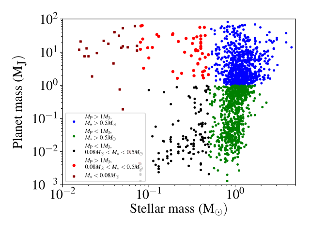
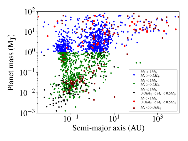
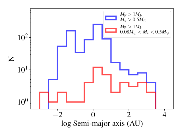
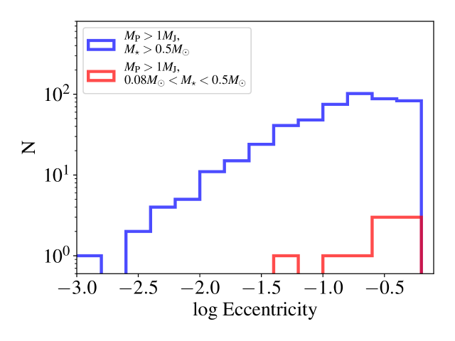
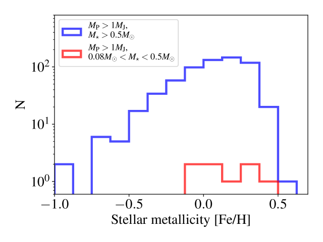
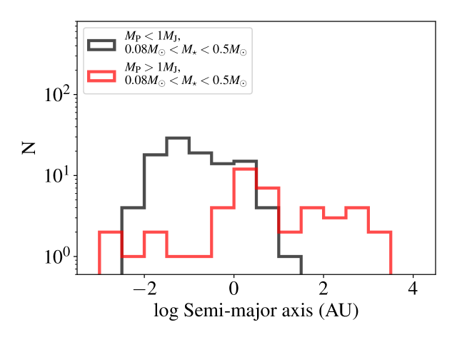
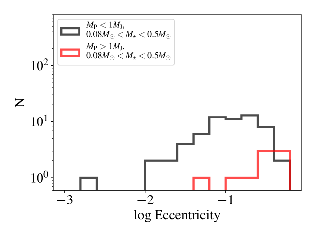
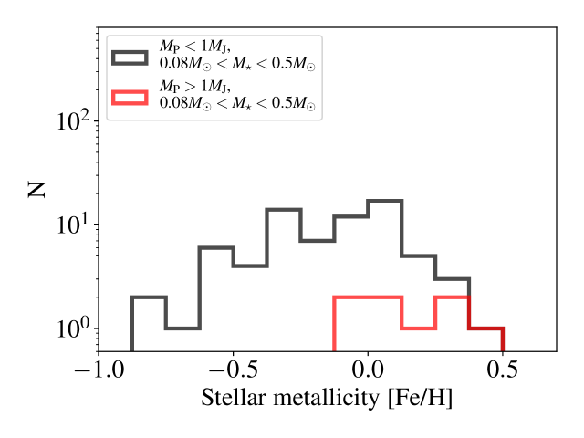
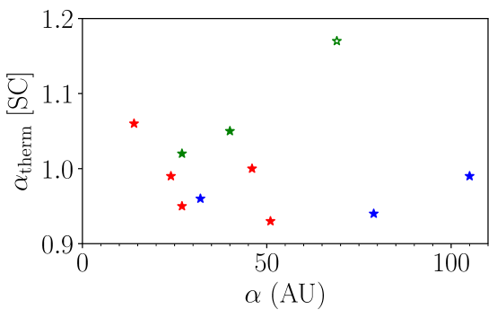
The planets around M dwarfs are diverse (see Figures 3-3). They have small to high masses (from Earth-mass planets to 13$\textup{ M}_{\textsc{j}}$-mass planets) and narrow to wide separations from their host stars ($10^{-3}$ to $10^{4}$ AU) (see Figure 3). A fraction of those planets ($\sim 30$%) are gas giants with a mass larger than 1$\textup{ M}_{\textsc{j}}$. Such massive planets are observed both near and far from their host star (Figure 3), whereas their eccentricities and metallicities seem to be rather high when they are compared with low-mass planets around M dwarfs and also when they are compared with high-mass planets around more massive stars (see Figures 3-3). It is therefore of interest to investigate how these giant planets around M dwarfs form.

(a)

(b)

Figure 1: Properties of the observed exoplanets around M dwarfs compared with the properties of all observed exoplanets. Red: companions (exoplanets and brown dwarfs up to $60\textup{ M}_{\textsc{j}}$) with $M_{\rm P}>1\textup{ M}_{\textsc{j}}$ around M dwarfs ($M_{\star}<0.5\textup{ M}_{\odot}$). Black: exoplanets with $M_{\rm P}<1\textup{ M}_{\textsc{j}}$ around M dwarfs. Blue: companions with $M_{\rm P}>1\textup{ M}_{\textsc{j}}$ around higher mass stars ($M_{\star}>0.5\textup{ M}_{\odot}$). Green: exoplanets with $M_{\rm P}<1\textup{ M}_{\textsc{j}}$ around higher mass stars ($M_{\star}>0.5\textup{ M}_{\odot}$). Brown: companions around brown dwarfs ($M_{\star}<0.08\textup{ M}_{\odot}$). Data taken from https://exoplanet.eu/(Schneider et al., 2011). This database uses the Hatzes & Rauer (2015) definition for planets (based on the mass-density relationship) and so it includes objects with masses $13-60\textup{ M}_{\textsc{j}}$, which would be classified as brown dwarfs according to their mass. The inclusion of these objects does not affect the discussion presented in this paper.

(a)

(b)

(c)

Figure 2: Comparison of the properties (semi-major axis, eccentricity and stellar metallicity) of high-mass exoplanets around M dwarfs with the properties of high-mass exoplanets around higher-masss stars (colours as in Figure 3). Exoplanets around M dwarfs (red histograms) tend to have high eccentricities and high metallicities.

(a)

(b)

(c)

Figure 3: Comparison between the properties (semi-major axis, eccentricity and stellar metallicity) of high-mass and low-mass exoplanets around M dwarfs (colours as in Figure 3). High-mass exoplanets (red histograms) tend to have high eccentricities and high metallicities when compared to their lower-mass counterparts.

Planets are believed to form by the core accretion scenario in which dust particles coagulate into progressively larger aggregates until a solid core forms, which can then promote the accretion of a gaseous envelope (Safronov & Zvjagina, 1969; Goldreich & Ward, 1973; Greenberg et al., 1978; Hayashi et al., 1985; Lissauer, 1993). In this scenario, the formation of giant planets needs a few Myr, a timescale that may exceed the lifetime of the disc (Haisch et al., 2001; Cieza et al., 2007), although the process of pebble accretion may accelerate the process (Lambrechts & Johansen, 2012).

An alternative theory of planet formation is disc instability, that is, planet formation by the gravitational fragmentation of young protostellar discs (Kuiper, 1951; Cameron, 1978; Boss, 1997). Fragmentation happens provided that the Toomre criterion (Toomre, 1964) is satisfied,

$$Q\equiv\frac{c_{s}(R)\kappa(R)}{\pi G\Sigma(R)}\stackrel{{\scriptstyle<}}{{{}_{\sim}}}1,\,$$ (1)

where $c_{\rm s}(R)$ is the sound speed, $\kappa(R)$ is the epicyclic frequency, and $\Sigma(R)$ is the surface density of the disc at a given orbital radius $R$. The gravitational instability leads to the formation of spiral arms that transfer angular momentum radially outwards. A spiral arm can evolve non-linearly and collapse if the cooling rate is sufficiently short: typically $t_{\textup{cool}}<(0.5-2)t_{\textup{orb}}$, that is, of the order of a few orbital periods (Gammie, 2001; Johnson & Gammie, 2003; Rice et al., 2003, 2005). In this scenario protoplanets form on a dynamical timescale (a few thousand years) and have initial masses of a few $\textup{M}_{\textsc{j}}$ (set by the opacity limit for fragmentation). However, these planets can rapidly accrete gas, growing in mass to become brown-dwarfs or low-mass hydrogen-burning stars (Stamatellos & Whitworth, 2009b; Kratter et al., 2010; Vorobyov, 2013; Kratter & Lodato, 2016). Those objects that do end up as planets are typically the ones that are ejected from the disc through gravitational interactions (Li et al., 2015, 2016; Mercer & Stamatellos, 2017).

Observations of young discs have revealed the presence of multiple gaps and bright rings at mm wavelengths (e.g. HL Tau, ALMA Partnership et al., 2015). Such gaps may be due to young planets (Dipierro et al., 2015), which opens up the possibility that planets may form on a short timescale. This idea is also corroborated by observations of later phase (T Tauri) discs, which show that at their present age (a few Myr) they do not have enough mass to form the observed population of exoplanets (Greaves & Rice, 2010; Manara et al., 2018). Rapid planet formation due to disc instability has been boosted by ALMA observations of massive extended discs in the Class 0 phase (Tobin et al., 2016) and of discs with spiral arms indicative of gravitational instabilities (Pérez et al., 2016; Tobin et al., 2016).

The existence of massive planets on wide orbits around M dwarfs poses challenges to both planet formation theories. M dwarf discs have lower masses than the discs around solar-type stars ($M_{\rm d}\approx M_{*}^{-2.4}$, e.g. Andrews et al., 2013; Mohanty et al., 2013; Ansdell et al., 2017; Stamatellos & Herczeg, 2015); disc masses are typically below a few $\textup{ M}_{\textsc{j}}$ (Ansdell et al., 2017; Manara et al., 2018), with evidence of quicker disc dissipation (Ansdell et al., 2017). Such low mass discs are not susceptible to disc fragmentation nor do they provide a good environment for pebble accretion (Liu et al., 2019).

It is possible though that these discs were more massive during their early phases, maybe massive enough for disc instability to operate and form giant planets fast. There are observations of planetary systems with a massive exoplanet with massx M$\sim\textup{ M}_{\textsc{j}}$ around a $\sim 100\textup{ M}_{\textsc{j}}$ star (see Figure 3). This means that the initial disc mass was at least 10% of the mass of the host star. However, this fraction could be much higher if one considers that (i) there may be other planets in the system that have not been detected, (ii) the stellar mass increases with time as it accretes gas from the disc, and (iii) a significant fraction of the disc mass may be lost due to accretion onto the host star, photoevaporation or disc winds. Therefore, disc instability may be a good candidate for explaining the formation of massive planets around M dwarfs, like for example, the planet around star GJ 3512 (Morales et al., 2019).

Massive planets on wide orbits around M dwarfs are ideal candidates for formation by disc instability as the conditions for the instability to happen are met in the outer disc regions (e.g. Stamatellos et al., 2007a; Stamatellos & Whitworth, 2009b; Stamatellos et al., 2011). Observational surveys indicate that only a small fraction of M dwarfs (less than $\sim 10\%$) host wide orbit planets and this also holds for higher-mass stars (Brandt et al., 2014; Bowler et al., 2015; Lannier et al., 2016; Reggiani et al., 2016; Galicher et al., 2016; Bowler, 2016; Vigan et al., 2017; Baron et al., 2018; Stone et al., 2018; Wagner et al., 2019; Nielsen et al., 2019) (see review by Bowler & Nielsen, 2018). These surveys typically explore a region out to a few hundred AU from the central star (or even a few thousand AU, Durkan et al., 2016; Naud et al., 2017) and they are sensitive down to Jupiter-mass planets. The occurrence rates of giant planets on wide orbits are uncertain as they depend upon the sensitivity limits derived from models of planet evolution and the assumptions made about the planet mass-period distribution (see Bowler & Nielsen, 2018). Nevertheless, it seems unlikely that giant planets on wide orbits are common. This implies a formation process that operates only in a small subset of disc initial conditions. Alternatively, the low-fraction of wide-orbit planets may be due to subsequent dynamical evolution, either migration towards the star due to disc-planet interactions (e.g. Stamatellos & Inutsuka, 2018), scattering farther away from the central star and/or ejection due to 3-body interactions (e.g. Mercer & Stamatellos, 2017) or disruption and ejection due to interactions within a cluster (Hao et al., 2013; Cai et al., 2017).

Disc instability in M dwarf discs has not been extensively studied. Boss (2006) suggests that the formation of Jupiter mass planets is possible via fragmentation of discs around stars with masses $0.1$ and $0.5\textup{ M}_{\odot}$. The discs that this author studies are small in extent ($4<R<20$ AU), so it is uncertain how the fast cooling needed for disc fragmentation is achieved. Backus & Quinn (2016) perform simulations of discs around a $0.33\textup{ M}_{\odot}$ star. They find that only the discs which exhibit $Q_{\textup{crit}}\lesssim 0.9$, fragment. The radii of the discs studied are between 0.3 and 30 AU, with masses between 0.01 and 0.08$\textup{ M}_{\odot}$. This study focuses on locally isothermal discs, which are more prone to fragmentation even at small radii given the fact that fragments can cool to the background temperature instantaneously, therefore artificially satisfying the cooling criterion for fragmentation.

In this paper, we improve upon previous studies by investigating the fragmentation of discs around M dwarfs using radiative hydrodynamic simulations with appropriate cooling. Our aim is two-fold: (i) to find the minimum disc mass required for fragmentation to happen, and (ii) to determine the properties of the planets that form and provisionally compare them with the observed properties of exoplanets around M dwarfs.

The paper is laid out as follows. In Section 2, we describe the numerical methods employed within the paper. Section 3 outlines the initial conditions of each simulation and Section 4 presents the tests performed to check the validity of our method. In Section 5 we discuss how different parameters affect the disc fragmentation mass. We investigate the properties of the formed planets in Section 6, and in Section 7 we compare these properties with exoplanet observations. Finally, the work is summarised in Section 8.

2 Numerical methods

We study the dynamics of fragmentation of protostellar discs around M dwarfs by performing hydrodynamic simulations of initially gravitationally stable discs that progressively increase in mass and fragment. In the following subsections we describe in detail the methods that we used.

2.1 Hydrodynamics

We utilized the code GANDALF (Hubber et al., 2018) to perform smoothed particle hydrodynamical simulations. The code uses the conservative grad-h SPH scheme (Springel & Hernquist, 2002). The Cullen & Dehnen (2010) implementation of time-dependent viscosity was utilised in order to reduce artificial viscosity away from shocks. An M4 cubic spline kernel (Schoenberg, 1946; Monaghan & Lattanzio, 1985) was used as the smoothing function.

The radiative transfer processes that regulate cooling and heating in the disc were treated with the method of Lombardi et al. (2015), which is based on the method of Stamatellos et al. (2007b) (see also Forgan et al., 2009). This method uses the gas pressure scale-height of a particle $i$, $H_{\textup{P},i}$ to obtain the column density, through which heating and cooling happens. The pressure scale-height is calculated using

$$H_{\textup{P},i}=\frac{P_{i}}{\rho_{i}\left|\boldsymbol{a}_{h,i}\right|},$$ (2)

where $P_{i}$ and $\rho_{i}$ are the pressure and density of the gas respectively. $\boldsymbol{a}_{h,i}$ is the hydrodynamical acceleration of the gas (i.e. the gravitational or viscous accelerations are not included). The column density of particle $i$ is then set to

$$\bar{\Sigma}_{i}=\zeta^{\prime}\rho_{i}H_{\textup{P},i},$$ (3)

where $\zeta^{\prime}=1.014$ is a dimensionless coefficient with a weak dependence on the polytropic index. This formulation has been shown to yield a more accurate estimate of the particle column density in the context of protostellar discs when compared to the method that uses the gravitational potential (Mercer et al., 2018).

Once the column density is calculated the heating/cooling rate of a particle $i$ is set to

$$\frac{\mathrm{d}u_{i}}{\mathrm{d}t}=\frac{4\sigma_{\textsc{sb}}\left(T^{4}_{\textsc{bgr}}-T^{4}_{i}\right)}{\bar{\Sigma}^{2}_{i}\kappa_{\textsc{r}}(\rho_{i},T_{i})+\kappa_{\textsc{p}}^{-1}(\rho_{i},T_{i})}.$$ (4)

$\sigma_{\textsc{sb}}$ is the Stefan-Boltzmann constant and $T_{\textsc{bgr}}$ is a background temperature that particles cannot radiatively cool below. $\kappa_{\textsc{r}}$ and $\kappa_{\textsc{p}}$ are the pseudo-mean Rosseland- and Planck opacities (see Lombardi et al., 2015, for details), respectively, and are assumed to be the same. Equation (4) allows the calculation of the cooling rate smoothly between the optically thin and thick regimes, whereas at the optically thick regime it reduces to the diffusion approximation (Mihalas, 1970).

We used the Bell & Lin (1994) opacities such that $\kappa(\rho,T)=\kappa_{0}\rho^{a}T^{b}$, where $\kappa_{0}$, $a$ and $b$ are constants set depending on the chemical species contributing to the opacity at a given density and temperature. Ice melting, dust sublimation, bound-free, free-free and electron scattering interactions are taken into account. We also used a detailed equation of state for the gas that considers the rotational and vibrational degrees of freedom of $\textup{H}_{2}$, the dissociation of $\textup{H}_{2}$,  and the ionisation of hydrogen and helium (see Stamatellos et al., 2007b, for details).

2.2 Mass loading

In order to find the minimum fragmentation mass of an M dwarf disc, we started with a graviationally stable disc and slowly increased its mass at a constant rate, employing a low mass accretion rate (see Zhu et al., 2012). The method can be conceptually thought as accretion onto the disc from an infalling envelope, where material is distributed across the whole disc. We set the disc mass accretion rate to

$$\dot{M}_{\textup{disc}}=\frac{\chi M_{\textup{disc,0}}}{t_{\textup{orb}}},$$ (5)

where $M_{\textup{disc, 0}}$ is the initial disc mass and $\chi$ is a factor which regulates the magnitude of accretion. $t_{\textup{orb}}$ is the orbital period of the disc at a radius $R=100$ AU, where

$$t_{\textup{orb}}=2\pi\sqrt{\frac{R^{3}}{GM_{\star}}}.$$ (6)

Therefore, $\chi$ represents the fraction of the increase of the disc mass during approximately one rotation at its initial outer edge. The mass accretion is simply performed by increasing the mass of every particle equally every timestep. We refer to this method as mass loading. The discs were evolved until they fragmented, which we define as when a density of $\rho>10^{-9}\textup{ g cm}^{-3}$ is attained. This value is around the density where the first hydrostatic core forms during the collapse (Larson, 1969; Stamatellos et al., 2007b). By chosing a relatively high density threshold like this, we ensured that bound objects formed (i.e. the disc fragments) rather than just transient over-densities. The density of the first core (when it forms) does not vary significantly with the core mass (Stamatellos & Whitworth, 2009a), therefore the same value can be used for all fragments forming in the disc, irrespective of their mass. From a practical point of view, the highest density SPH particle wass identified at each timestep and its density was compared with the threshold density (the SPH particle density is calculated using $\sim 50$ neighbourghing particles). The centre of the clump was found by the position of the highest density particle within it (usually there were $\sim 10^{5}$ particles within each clump, see Section 6).

One caveat of the mass loading method is that higher density regions of the disc (i.e. where there are more particles) are preferentially mass-loaded. For example, spiral arms may receive a higher proportion of the accreted mass and the collapse of a dense region may be driven artificially, if the accretion rate is set too high . We therefore used a relatively low disc accretion rate (see tests below) so that accretion is not the key driver of the gravitational instability (e.g. Hennebelle et al., 2016).

Table 1: Initial conditions of the disc simulations: initial stellar mass ($M_{\star,0}$), disc radius ($R_{\textup{init}}$), metallicity ($z$), disc mass ($M_{\textup{disc, 0}}$), and mass loading rate ($\dot{M}_{\textup{disc}}$). Disc masses were set such that the Toomre parameter at the outer disc radius is $Q=10$ (i.e. the discs are initially gravitationally stable). The constant mass loading rate onto the disc was set from Equation 5, where $\chi=0.1$. The disc metallicity was varied by modifying the opacities by a factor $z$.

Run	$M_{\star,0}$ ($\textup{M}_{\odot}$)	$R_{\textup{init}}$ (AU)	$z$	$M_{\textup{disc, 0}}$ ($\textup{M}_{\odot}$)	$\dot{M}_{\textup{disc}}\leavevmode\nobreak\ (10^{-6}\textup{ M}_{\odot}\textup{ yr}^{-1}$)
01	0.2	60	1	0.040	1.80
02	0.2	60	0.1	0.040	1.80
03	0.2	60	10	0.040	1.80
04	0.2	90	1	0.050	2.25
05	0.2	90	0.1	0.050	2.25
06	0.2	90	10	0.050	2.25
07	0.2	120	1	0.059	2.63
08	0.2	120	0.1	0.059	2.63
09	0.2	120	10	0.059	2.63
10	0.3	60	1	0.049	2.70
11	0.3	60	0.1	0.049	2.70
12	0.3	60	10	0.049	2.70
13	0.3	90	1	0.062	3.38
14	0.3	90	0.1	0.062	3.38
15	0.3	90	10	0.062	3.38
16	0.3	120	1	0.072	3.95
17	0.3	120	0.1	0.072	3.95
18	0.3	120	10	0.072	3.95
19	0.4	60	1	0.057	3.60
20	0.4	60	0.1	0.057	3.60
21	0.4	60	10	0.057	3.60
22	0.4	90	1	0.071	4.50
23	0.4	90	0.1	0.071	4.50
24	0.4	90	10	0.071	4.50
25	0.4	120	1	0.083	5.26
26	0.4	120	0.1	0.083	5.26
27	0.4	120	10	0.083	5.26

3 Initial conditions

Figure 4: Toomre parameter, $Q$ as a function of the radius for discs with outer extents $R_{\textup{init}}=[60,\leavevmode\nobreak\ 90,\leavevmode\nobreak\ 120]$ AU. The dashed black line represents a value of $Q=10$, the Toomre parameter value at the disc outer edge. Each disc is initially stable at all radii.

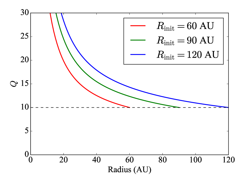
We constructed protostellar systems consisting of M dwarfs attended by discs with different stellar mass, disc radial extent and metallicity (see Table 1). The stellar masses were set to $M_{\star}=[0.2,\leavevmode\nobreak\ 0.3,\leavevmode\nobreak\ 0.4]\textup{ M}_{\odot}$ exploring a range of masses for M dwarfs. The initial disc radii were set to $R_{\textup{init}}=[60,\leavevmode\nobreak\ 90,\leavevmode\nobreak\ 120]$ AU, whereas the discs’ inner edge was set to $5$ AU. The metallicity was varied by modifying the opacities by factors of $z=[0.1,1,10]$. The initial disc mass was chosen such that the Toomre parameter has a fixed value at the outer radius of the disc ($Q_{\textup{out}}=10$). This ensures that the discs are initially gravitationally stable (see Figure 4). Each disc was comprised of $N\approx 2\times 10^{6}$ SPH particles, so that both the Jeans mass and the Toomre mass were well resolved (Bate & Burkert, 1997; Nelson, 2006; Stamatellos & Whitworth, 2009a). Similarly, the disc vertical structure was adequately resolved; for the number of SPH particles that we used the disc scale height is generally at least $\sim 10$ smoothing lengths (see Stamatellos & Whitworth, 2009a).

The surface density and temperature profiles of the disc were set to $\Sigma\propto R^{-p}$ and $T\propto R^{-q}$, respectively. The surface density power index $p$ is thought to lie between 1 and $3/2$ from semi-analytical studies of cloud collapse and disc creation (Lin & Pringle, 1990; Tsukamoto et al., 2015; MacFarlane & Stamatellos, 2017). The temperature power index $q$ ranges from $0.35$ to $0.8$ as derived from observations of pre-main sequence stars (Andrews et al., 2009). Here, we adopted $p=1$ and $q=0.7$. The exact initial surface density profile that we used is

$$\Sigma(R)=\Sigma_{0}\left(\frac{R_{0}^{2}}{R^{2}+R_{0}^{2}}\right)^{1/2},$$ (7)

where $\Sigma_{0}$ is the surface density 1 AU away from the star and $R_{0}=0.01$ AU is a smoothing radius to prevent unphysically high values close to the star. The disc initial temperature profile was set to

$$T(R)=\left[T^{2}_{0}\left(\frac{R^{2}+R^{2}_{0}}{\textup{AU}^{2}}\right)^{-0.7}+T_{\infty}^{2}\right]^{1/2}.$$ (8)

Here, $T_{0}=100$ K is the temperature at 1 AU from the star and $T_{\infty}=10$ K is the temperature far away from the star. This profile were also used to provide a minimum temperature below which SPH particles cannot radiatively cool, that is, $T_{\textsc{bgr}}$ in Equation 4.

Figure 5: Convergence test for the mass loading method described in Section 2. We performed SPH simulations with an increasing number of particles and compared the disc mass at the point of fragmentation. We see that for $>128\times 10^{3}$ particles, there is little difference in the fragmentation mass of the disc. We therefore conclude that the method is well converged for $N\approx 2\times 10^{6}$, the number of particles used for the simulations presented in this work.

4 Method tests

4.1 Test 1: Disc fragmentation mass

To check the validity of the mass loading method as a good way to estimate the fragmentation minimum disc mass, we performed a simulation of a disc around an M dwarf of mass $0.2\textup{ M}_{\odot}$, where the initial disc mass was set to $0.12\textup{ M}_{\odot}$ and the disc accretion rate to $3\times 10^{-5}\textup{ M}_{\odot}\textup{ yr}^{-1}$ that is, $\chi=0.5$ (see Equation 5). We also performed a set of simulations where the disc masses are fixed (i.e. without any mass loading), but in each simulation the disc had mass from $0.15$ to $0.2\textup{ M}_{\odot}$, in $0.01\textup{ M}_{\odot}$ intervals. Each disc had surface density and temperature profiles of $\Sigma\propto R^{-1}$ and $T\propto R^{-0.7}$ respectively, extends from 5 to 90 AU, and were comprised of $N\approx 2\times 10^{6}$ particles. We found that the disc with a fixed mass of $0.17\textup{ M}_{\odot}$ does not undergo fragmentation whereas the disc with a fixed mass of $0.18\textup{ M}_{\odot}$ did. The disc in the simulation that included mass loading fragmented at a mass of $0.176\textup{ M}_{\odot}$, consistent with fixed-mass disc simulations.

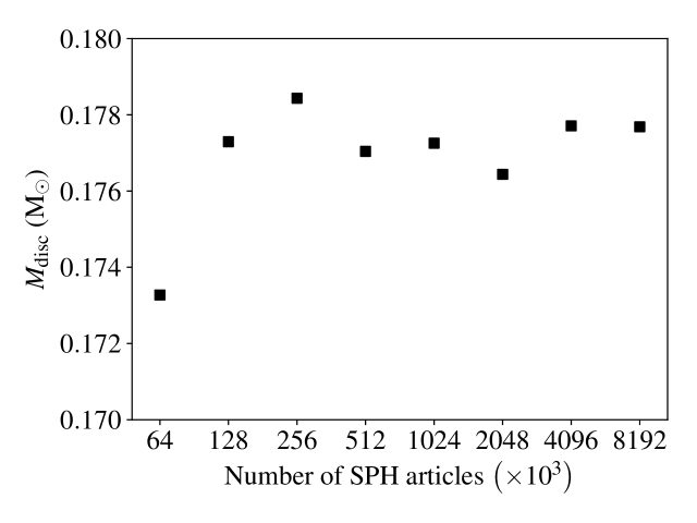
4.2 Test 2: Mass loading convergence

We performed a set of simulations with the same parameters as the simulation with mass loading described above, but with an increasing number of SPH particles in order to check for convergence. Figure 5 shows the mass at which a disc fragmented under mass loading with an increasing number of particles. Even for a relatively small number of particles $\left(N=128,000\right)$ we achieved convergence. Only negligible differences were seen when the particle number is consequently doubled, up to a maximum of $N\approx 8\times 10^{6}$.

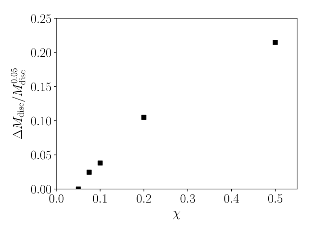
4.3 Test 3: Mass loading and choice of accretion rate

We investigated the effect of the factor which regulates the amount of mass loading, $\chi$ (see Equation 5). We chose a disc with properties (mass, radius, metallicity) the same as the disc of Rxun 4 in Table 1, and we performed simulations with different accretion rates. Figure 6 shows the fractional difference in the disc fragmentation masses for $\chi=[0.05,0.075,0.1,0.2,0.5]$. The corresponding mass accretion rates are $\dot{M}_{\textup{disc}}=[1.25,1.88,2.5,5,12.5]\times 10^{-6}\textup{ M}_{\odot}\textup{ yr}^{-1}$. We need to use a low accretion rate onto the disc so that its evolution is not affected by the mass loading, whereas for computational purposes we need to have a high accretion rate so that the fragmentation mass is achieved quickly. There is little difference ($\leq 5\%$) in the computed fragmentation mass for $\chi\leq 0.1$ and so this is the value we adopted for the rest of the work presented in this paper. It is important to note that the difference in the disc fragmentation mass between $\chi=0.05$ and $\chi=0.5$ is relatively small ($\sim 20\%$ ).

Figure 6: Fractional difference in the disc fragmentation mass for different values of the parameter $\chi$, which regulates the disc accretion rate (see Equation 5). The reference value is the disc fragmentation mass for $\chi=0.05$ (denoted as $M_{\mathrm{disc}}^{0.05}$). The corresponding mass accretion rates for $\chi=[0.05,0.075,0.1,0.2,0.5]$ are $\dot{M}_{\textup{disc}}=[1.25,1.88,2.5,5,12.5]\times 10^{-6}\textup{ M}_{\odot}\textup{ yr}^{-1}$, respectively. We show that for values of $\chi\leq 0.1$, there is only a small difference ($\leq 5\%$) in the disc fragmentation mass. As such, a value of $\chi=0.1$ is adopted for the work presented here. The difference in the disc fragmentation mass between $\chi=0.05$ and $\chi=0.5$ is relatively small ($\sim 20\%$ ).

5 Fragmentation of M dwarf discs

We performed a set of 27 simulations, varying the initial disc mass, disc radius, metallicity, and the mass of the host star. Each disc was initially gravitationally stable, but its mass increased over time through mass loading (see Section 2). As such, each disc eventually became unstable and spiral arms developed. In the majority of cases, continued mass loading caused the spiral arms to evolve non-linearly, and to ultimately form gravitationally bound fragments.

The results of the disc simulations are presented in Table 2. When a disc fragments, its mass yields the minimum disc mass for fragmentation, which we denote as $M_{\textup{disc}}$. We also calculated the time of fragmentation $t$, the disc-to-star mass ratio when fragmentation happens $q$, and the radius of the disc $R_{\textup{disc}}$, which encompasses $95\%$ of the disc mass. The distance between the central star and the formed fragment is denoted as $a_{\textup{frag}}$. In the table we also state the stellar mass and and the disc-to-star mass ratio when fragmentation happens.

Table 2: Results for the disc simulations with the initial conditions listed in Table 1 after 30 kyr of evolution. $M_{\star}$ and $M_{\textup{disc}}$ are respectively the masses of the star and disc when the disc fragments. $t$ is the time at which fragmentation occurs, $q$ is the disc-to-star mass ratio at fragmentation and $R_{\textup{disc}}$ is the radius of the disc. $a_{\textup{frag}}$ is the distance of the fragment from the host star. Some discs did not fragment as noted by dashes in the corresponding rows.

Run	$M_{\star}$ ($\textup{M}_{\odot}$)	$M_{\textup{disc}}$ ($\textup{M}_{\odot}$)	$\Delta M_{\textup{disc}}$ ($\textup{M}_{\textsc{j}}$)	$t$ (kyr)	$q$	$R_{\textup{disc}}$ (AU)	$a_{\textup{frag}}$ (AU)
01	0.205	0.075	36.6	22.1	0.37	75	49
02	0.205	0.077	38.9	23.3	0.38	72	35
03	-	-	-	-	-	-	-
04	0.205	0.104	56.2	25.9	0.51	92	54
05	0.206	0.105	57.2	27.6	0.51	137	55
06	0.207	0.106	58.1	28.0	0.51	169	32
07	0.204	0.124	68.7	26.7	0.61	144	46
08	0.205	0.126	70.8	27.6	0.62	128	30
09	0.207	0.128	72.2	28.8	0.62	190	54
10	0.305	0.094	46.9	18.5	0.31	96	40
11	0.305	0.097	50.2	19.6	0.32	68	32
12	-	-	-	-	-	-	-
13	0.305	0.122	63.0	19.2	0.40	89	59
14	0.305	0.125	66.3	20.2	0.41	89	28
15	-	-	-	-	-	-	-
16	0.304	0.146	77.8	20.0	0.48	131	55
17	0.305	0.150	81.7	21.0	0.49	126	60
18	0.307	0.155	86.7	22.7	0.50	159	84
19	-	-	-	-	-	-	-
20	-	-	-	-	-	-	-
21	-	-	-	-	-	-	-
22	0.405	0.144	76.2	17.3	0.36	105	57
23	0.405	0.140	72.1	16.4	0.35	91	37
24	-	-	-	-	-	-	-
25	0.405	0.165	86.1	16.5	0.41	123	47
26	0.405	0.171	91.6	17.6	0.42	130	43
27	0.407	0.176	97.4	19.0	0.43	164	116

Fragmentation happens quite fast, within a few tens of kyr ($\sim 16-28$ kyr; see Table 2). The discs generally fragment at distances $>30$ AU from the host star; the most likely distance for fragmentation to happen is $50-60$ AU (see Figure 7). This is closer to the central star than for fragmentation of discs around more massive stars; Stamatellos & Whitworth (2009b) find a most likely distance of $100-150$ AU, for massive discs around 0.7-$\textup{M}_{\odot}$ stars. This is consistent with the expectation that discs around less massive stars fragment closer to the central star, $a_{\rm fragm}\propto\left({M_{\star}}/{\textup{M}_{\odot}}\right)^{1/3}$ (Whitworth & Stamatellos, 2006). According to this relation one would expect the optimal region for fragmentation around M dwarfs to be around 75-100 AU, which is larger than what we find here. However, this is expected as in the simulations of Stamatellos & Whitworth (2009b) a slightly different radiative transfer method is used (utilizing the gravitational potential of the particle to calculate the column density) which results in less efficient cooling, making fragmentation at a specific distance from the host star less likely than the method used here (utilizing the pressure scale height; see Mercer et al., 2018).

Figure 7: Probability distribution of the orbital radius of the first fragment that forms in each simulation. M dwarf discs are most likely to fragment at distances $50-60$ AU from the host star. The error bars correspond to the Poisson (statistical) error. Only 20 fragments formed in the simulations, therefore the uncentainties are rather large.

Figure 8: Surface density plots for a selection of discs at the time of fragmentation (i.e. when a density of $10^{-9}\textup{ g cm}^{-3}$ is reached). The fragments are shown by the white points. The initial conditions for each run can be found in Table 1 and the results in Table 2.

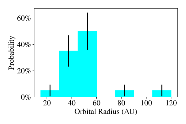
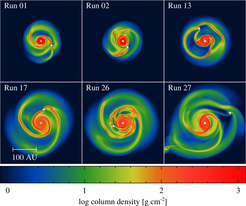
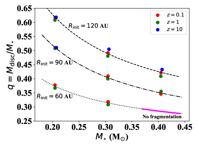
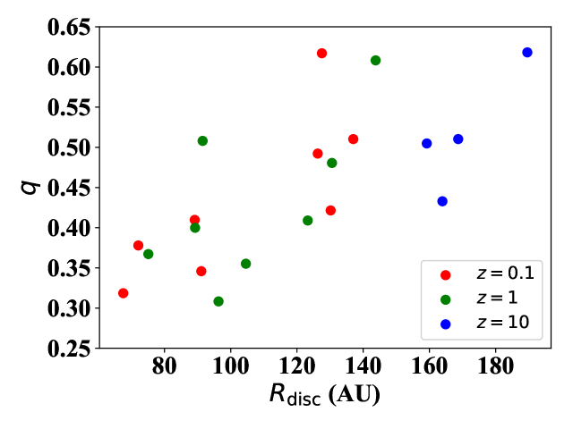
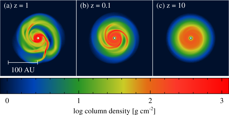
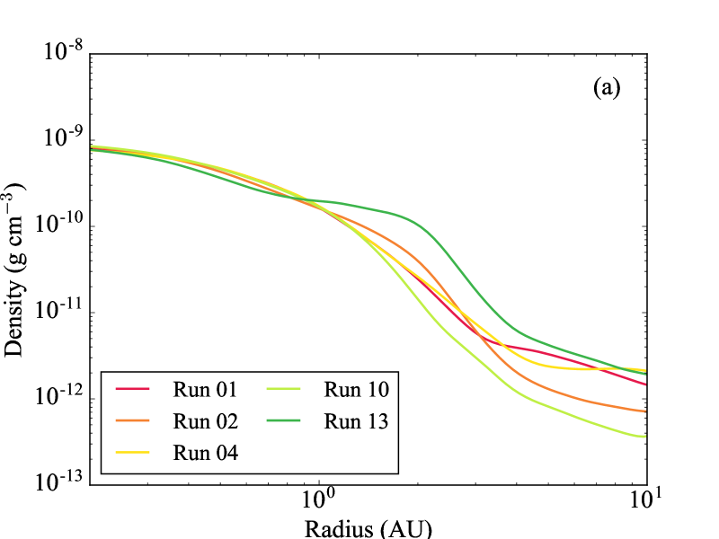
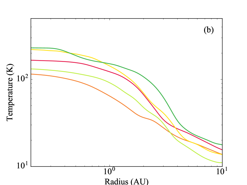
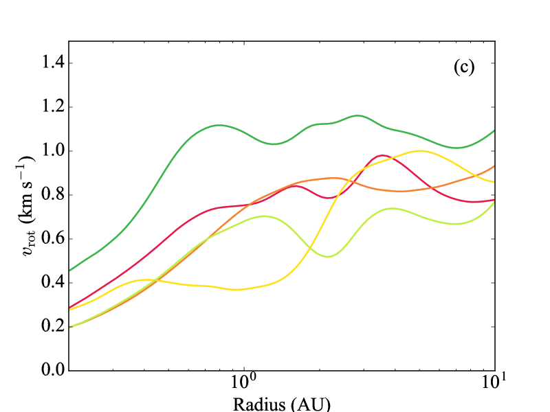
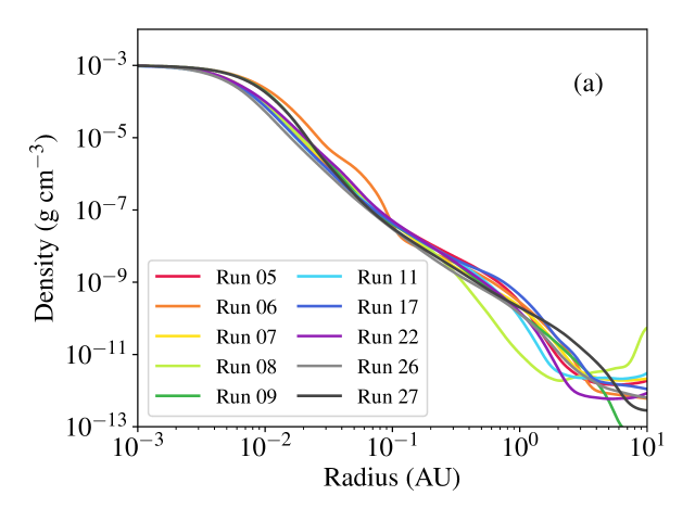
Figure 8 shows the surface density snapshots of six representative simulations at the time when the density at the center of the fragment is $10^{-9}\textup{ g cm}^{-3}$ (i.e. when, by definition, fragmentation has happened). In Figures 10-12, we present the relations between the different parameters that we investigated in this study (stellar mass, disc mass, disc radius, metallicity). In the following subsections we discuss these relations in detail.

5.1 The effect of the stellar mass and the disc radius

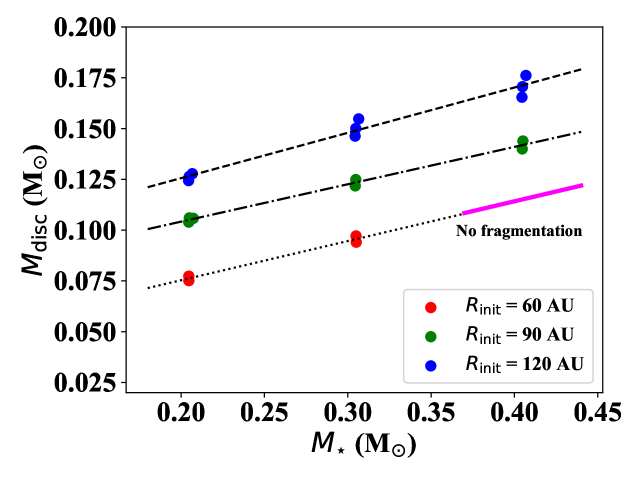
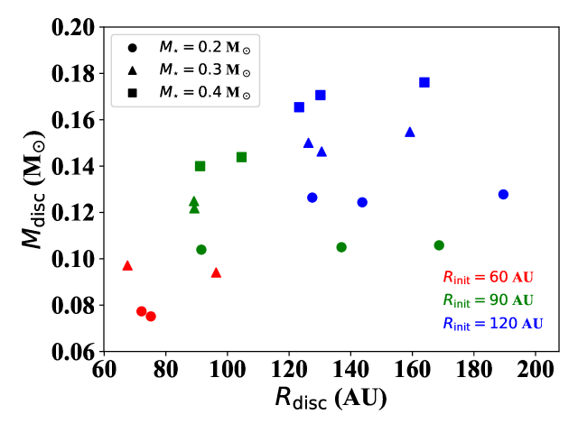
The disc fragmentation mass is shown as a function of the stellar mass in Figure 10, which demonstrates that for a given initial disc radius (60, 90, 120 AU), the disc fragmentation mass increases linearly with the stellar mass: $M^{\rm 60AU}_{\rm disc}=0.04+0.19M_{\star}$, $M^{\rm 90AU}_{\rm disc}=0.07+0.18M_{\star}$, $M^{\rm 120AU}_{\rm disc}=0.08+0.22M_{\star}$. A more massive central star results in a more stable disc as $Q\propto\Omega$ and $\Omega\propto M_{\star}^{1/2}$. The disc fragmentation mass also increases with the initial disc radius as the average surface density of smaller discs is larger for the same disc mass. Hence, smaller discs (but still discs with size $>70$ AU) fragment at a lower mass, as $\Sigma\propto R^{-1}$ and $Q\propto\Sigma^{-1}$ (see also Figure 10).

The disc-to-star mass ratio needed for fragmentation varies from $\sim 0.3$ (for small discs) to $\sim 0.6$ (for more extended discs) (see Figures 12-12). Therefore relatively large disc masses are needed for fragmentation to happen around M dwarfs. Such high disc masses have not been observed (Andrews et al., 2013; Mohanty et al., 2013; Ansdell et al., 2017), but it may be possible that M dwarf discs are more massive at their younger phase, as for example, the discs around solar-mass Class 0 objects (Dunham et al., 2014; Tobin et al., 2016). We also find that discs (with the same initial size) around more massive stars fragment at a lower disc-to-star mass ratio as the disc fragmentation mass increases slower than the stellar mass (see Figure 12).

Figure 9: Disc mass as a function of stellar mass when the disc fragments. Different colours correspond to different initial disc radii (as marked on the graph). The relationship between the two quantities is linear for a given initial disc radius. Smaller discs fragment at a lower mass, as the average disc surface density is larger. The different lines correspond to the linear relations derived for simulations with the same initial disc radius (see text). The purple line corresponds to the area in the parameter space where no fragmentation occurs (small discs around more massive M dwarfs).

(a)

Figure 10: Disc mass and as a function of disc radius at the time when the disc fragments. The disc radius is the radius which encompasses 95% of the disc mass. Generally speaking, a higher disc mass is required for fragmentation of more extended discs. Initial disc radii of $R_{\textup{init}}=[60,90,120]$ AU are shown by the red, green and blue points, respectively. The initial stellar masses of $M_{\star}=[0.2,0.3,0.4]\textup{ M}_{\odot}$ are denoted by the circles, triangles and squares, respectively. We note the difference between initial $R_{\textup{init}}$ and final disc radius $R_{\textup{disc}}$ (i.e. the disc radius when it fragments).

(a)

Figure 11: Disc-to-star mass ratio, $q$, at the time of disc fragmentation as a function of stellar mass for metallicities $z=[0.1,1,10]$ marked by the red, green and blue points, respectively. Each group of points (3 or 2 points) correspond to simulations of different metallicity discs (that have the same initial radius) around the stars with the same mass. We note that discs (with the same initial extent) around more massive stars fragment at a lower disc-to-star mass ratio. The disc-to-star mass ratio required for fragmentation varies from $\sim 0.3$ (for small discs) to $\sim 0.6$ (for more extended discs). The different lines correspond to the hyperbolic relations derived for simulations with the same initial disc radius. The purple line corresponds to the area in the parameter space where no fragmentation occurs (small discs around more massive M dwarfs).

(a)

Figure 12: Disc-to-star mass ratio, $q$, at the time of disc fragmentation as a function of the disc radius, for metallicities $z=[0.1,1,10]$ marked by the red, green and blue points, respectively. Discs with higher metallicity are larger when they fragment, suggesting a period of expansion. The required disc-to-mass ratio for fragmentation increases with disc size.

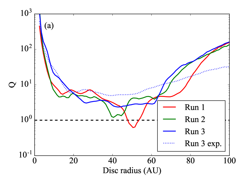
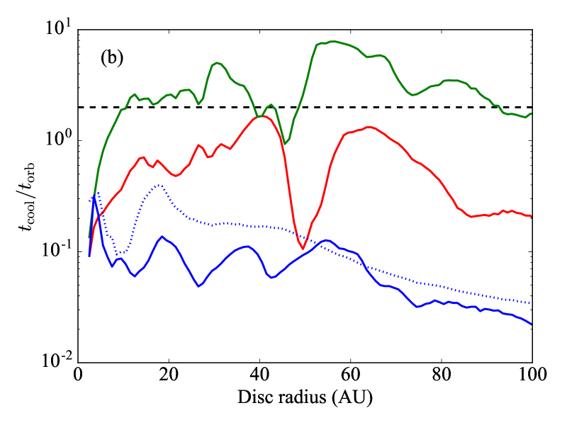
The discs in runs 19 - 21, which correspond to small discs ($R=60$ AU) around more massive M dwarfs ($M_{\star}=0.4\textup{ M}_{\odot}$) do not fragment. This also true for runs 3, 12, 15, and 24, which correspond to discs with high metallicity. We attribute this behaviour to a period of rapid disc expansion, a result of strong spiral arm formation and efficient outward transport of angular momentum which reduces the surface density and stabilises the discs. To demonstrate the effect of disc expansion, we compare runs 1 - 3; the disc in runs 1 and 2 undergo fragmentation, whereas the disc in run 3 exhibits rapid expansion. Figure 14 shows azimuthally-averaged Toomre parameter (a) and the cooling time in units of the local orbital period (b). Although in each case the cooling time is short enough to allow for a fragment to condense out, the disc in run 3 does not fragment due to rapid expansion (the spiral arms efficiently distribute angular momentum outwards).

5.2 The effect of metallicity

We examined three different values of the metallicity by modifying the opacities used in Equation 4 by factors of $z=[0.1,1,10]$. We find that changing the metallicity has little effect on the disc fragmentation mass for the disc with the same extent (see Figure 12) (although in some cases the disc does not fragment, see discussion below).

On the other hand, the disc evolution is affected by metallicity; from the onset of the gravitational instability, to the collapse of dense fragments (see Figures 14-14). In Figure 14, we present surface density snapshots of runs 1 - 3 (panels a, b and c respectively) at a time of 22 kyr. Figure 14a shows the disc shortly before fragmentation (for run 1, i.e. disc with solar metallicity, $z=1$). When the disc metallicity is lower ($z=0.1$; Figure 14b), the disc exhibits weaker, but well defined spiral features. Given that the optical depth $\tau=\Sigma\kappa$, and the metallicity has been reduced, more gas is required for the spiral arms to attain $\tau\sim 1$, where cooling is most efficient. As such, the spirals in this case take longer to fragment (see Table 2). However, once a sufficient surface density is reached, fragmentation occurs as cooling is efficient. When the disc metallicity is higher ($z=10$; Figure 14c), the disc does not fragment as it cannot cool fast enough; instead it expands and becomes gravitationally stable ($Q>1$), although it can then cool fast enough, as the surface density has decreased (see Figure 14).

In Figure 12, we present the relationship between the stellar mass and the disc-to-star mass ratio, and in Figure 12 the relationship between the disc fragmentation mass and the disc-to-star mass ratio, for different disc metallicities. In general, we find that metal rich discs fragment at a slightly higher disc-to-star mass ratio (Figure 12) and their corresponding discs are more extended when they fragment (Figure 12). We also find that the smaller ($R=[60,90]$ AU) discs with metallicity $z=10$ do not fragment (apart from run 6). This is due to period of fast disc expansion, when the spiral features become strong, combined with inefficient cooling (during the expansion phase). Runs 3, 12 and 15 are examples of this. This is the reason why the discs in the runs 19 - 21 as well as 24 do not fragment (see discussion in Section 5.1).

(a)

(b)

Figure 13: Azimuthally-averaged Toomre parameter (a) and the cooling time in units of the local orbital period (b) for runs 1 - 3 (red, green and blue, respectively). The time at which these quantities are shown are just prior to fragmentation (runs 1 and 2), and just prior to a period of disc expansion (run 3). The dashed blue line shows run 3 after the expansion. Each disc is gravitationally unstable such that spiral arms form, but only in runs 1 and 2 does the Toomre parameter fall below unity so that bound fragments form. In all cases, the cooling time is sufficiently short for a condensed fragment to collapse. The expansion of the disc in run 3 (and characteristic of most runs with an increased metallicity) acts to stabilise it.

Figure 14: Surface density of the discs in runs 1, 2, and 3, at 22 kyr (see Table 2). The disc in panel (a) has $z=1$ (solar metallicity), and is shown just prior to the formation of a bound fragment. The disc in panel (b) has a metallicity reduced by an order of magnitude ($z=0.1$). The disc is unstable but the spiral arms are not as strong as in disc in run 1. The disc in panel (c) has a metallicity increased by an order of magnitude ($z=10$). No strong spirals have formed yet. Spirals do eventually form, but the disc does not fragment due to a period of rapid expansion.

5.3 Accretion onto the central star

Figure 15: Relationship between the accretion rate onto the disc (Equation 5) and the accretion rate onto the central star. The black points show the average accretion for the entire simulation, whereas the red and blue points the average stellar rate during the first and last $10\%$ of the simulated time, respectively.

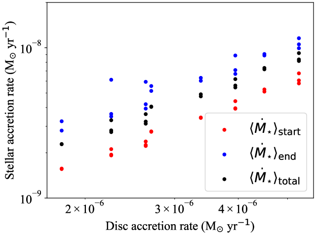
Typically, the mass accretion rate of the central star scales with the disc accretion rate, albeit $\sim 3$ orders of magnitude smaller. Figure 15 shows this relation. The disc accretion rate for each disc is set by Equation 5 and listed in Table 1. We show the average stellar accretion rate throughout the whole simulation, as well as the beginning and end of each simulation. We find that the stellar accretion rate is smaller at the start of each simulation and larger at the end, as compared to the total average accretion rate. Towards the end of the simulations, the discs are gravitationally unstable and accretion is enabled by outward angular momentum transfer due to gravitational torques. Prior to the onset of the instability, angular momentum transport outwards is inefficient, and material only moves inwards slowly.

6 The properties of protoplanets formed around M dwarfs by disc instability

Table 3: Properties of Type I and Type II protoplanets (see discussion in text). We list the Run ID, the type of protoplanet, the density at the centre of the protoplanet $\rho_{c}$, the time $\Delta t_{c}$ it took the protoplanet to collapse from density $10^{-9}{\rm g\ cm}^{-3}$ to its final central density, the distance of the protoplanet from the star, $a$, the first and second hydrostatic core radii ($R_{\textup{fc}}$ and $R_{\textup{sc}}$, respectively), the first and second hydrostatic core masses ($M_{\textup{fc}}$ and $M_{\textup{sc}}$, respectively), the number of SPH particles of the first core, which is indicative of how well the first core and its collapse are resolved, the ratios of rotational-to-gravitational $\beta_{\rm rot}$ and thermal-to-gravitational energies $\alpha_{\rm therm}$, for the first and second cores, and finally the specific angular momenta of the first and second cores.

Run	Type	$\rho_{c}$	$\Delta t_{c}$	$a$	$R_{\textup{fc}}$	$R_{\textup{sc}}$	$M_{\textup{fc}}$	$N_{\textup{fc}}$	$M_{\textup{sc}}$	$\beta_{\rm rot}^{\textup{fc}}$	$\alpha_{\rm therm}^{\textup{fc}}$	$\beta_{\rm rot}^{\textup{sc}}$	$\alpha_{\rm therm}^{\textup{sc}}$	$J_{\textup{fc}}$	$J_{\textup{sc}}$
		(${\rm g\ cm}^{-3}$)	(kyr)	(AU)	(AU)	($\textup{R}_{\odot}$)	($\textup{M}_{\textsc{j}}$)	($10^{5}$)	($\textup{M}_{\textsc{j}}$)					(cm2 s-1	$\times 10^{18}$)
01	IIb	$8.5\times 10^{-9}$	0.4	49	6.6	-	9.5	2.3	-	0.22	0.46	-	-	59	-
02	IIb	$1.8\times 10^{-7}$	0.3	24	2.3	-	6.5	1.6	-	0.21	0.48	-	-	18	-
04	IIb	$6.0\times 10^{-8}$	0.8	104	14	-	9.0	1.6	-	0.12	0.60	-	-	32	-
05	Ia	$10^{-3}$	1.0	27	3.2	7.3	9.2	1.6	2.6	0.12	0.80	0.07	0.95	21	0.3
06	Ia	$10^{-3}$	0.3	32	4.5	28	21	3.6	11	0.06	0.92	0.05	0.96	25	2.6
07	Ia	$10^{-3}$	0.7	27	3.7	5.8	10	1.5	2.8	0.08	0.86	0.05	1.02	18	0.2
08	Ia	$10^{-3}$	0.1	14	3.2	5.5	6.0	0.9	2.9	0.05	0.90	0.04	1.06	4.1	0.2
09	Ia	$10^{-3}$	1.1	105	7.1	6.1	13	1.8	5.0	0.08	0.88	0.06	0.99	24	0.5
10	IIb	$7.1\times 10^{-7}$	0.6	38	4.2	-	9.5	1.8	-	0.10	0.67	-	-	25	-
11	Ia	$10^{-3}$	0.3	24	2.3	5.9	6.9	1.3	2.4	0.10	0.84	0.06	0.99	10	0.2
13	IIa	$3.1\times 10^{-6}$	0.3	69	2.7	29	14	2.2	5.3	0.08	0.79	0.04	1.17	20	1.4
14	Ib	$10^{-3}$	0.2	18	2.8	-	6.1	0.9	-	0.10	0.86	-	-	4.3	-
16	Ib	$10^{-3}$	0.4	63	6.5	-	21	2.8	-	0.11	0.82	-	-	60	-
17	Ia	$10^{-3}$	0.5	51	4.5	8.8	11	1.4	2.6	0.13	0.78	0.08	0.93	26	0.2
18	Ib	$10^{-3}$	1.0	72	1.0	-	15	1.8	-	0.09	0.90	-	-	16	-
22	Ia	$10^{-3}$	0.6	40	3.1	6.4	9.7	1.3	3.5	0.07	0.87	0.04	1.05	10	0.2
23	Ib	$10^{-3}$	0.3	33	3.2	-	8.9	1.2	-	0.11	0.82	-	-	12	-
25	Ib	$10^{-3}$	0.6	49	6.2	-	16	1.8	-	0.11	0.83	-	-	46	-
26	Ia	$10^{-3}$	0.3	46	5.1	5.5	5.6	0.6	1.9	0.07	0.86	0.04	1.00	7.7	0.1
27	Ia	$10^{-3}$	1.7	79	8.9	7.6	17	1.7	4.9	0.10	0.86	0.09	0.94	49	0.5

The evolution of the discs that fragment was followed until the first fragment formed in each simulation collapsed further to densities higher than $10^{-9}\textup{ g cm}^{-3}$ (i.e. the limit we set for fragmentation in the previous section). These fragments are collectively referred to as protoplanets. It is expected that some of them evolve to become planets, whereas others get tidally disrupted and disperse or accumulate too much gas and become brown dwarfs (Stamatellos & Whitworth, 2009b; Kratter et al., 2010; Zhu et al., 2012).

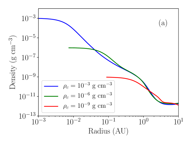
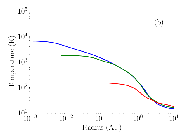
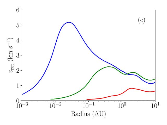
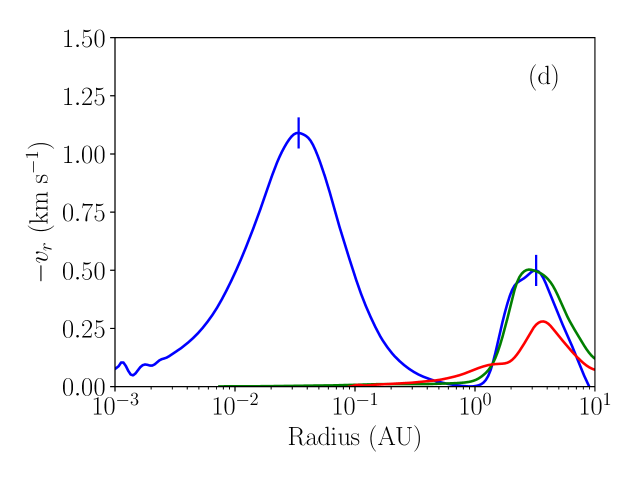
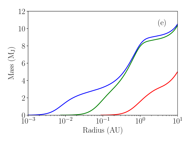
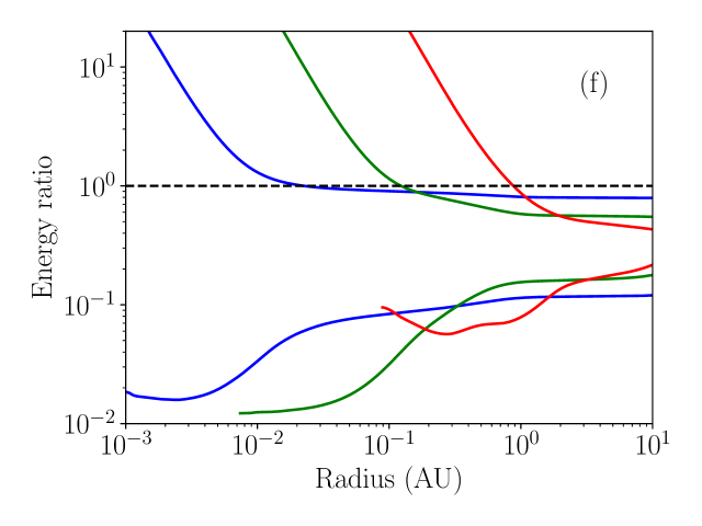
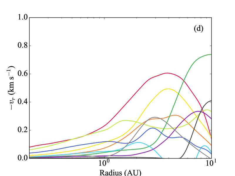
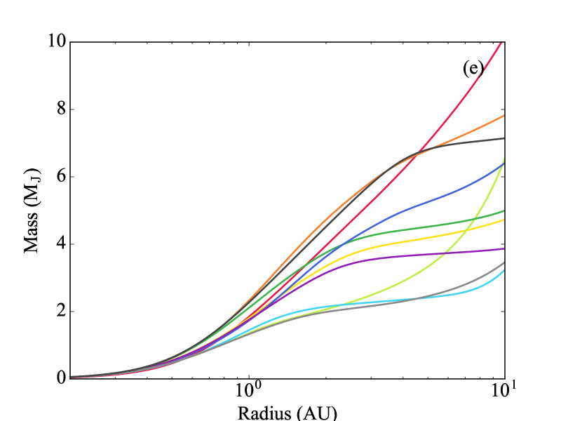
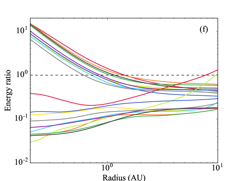
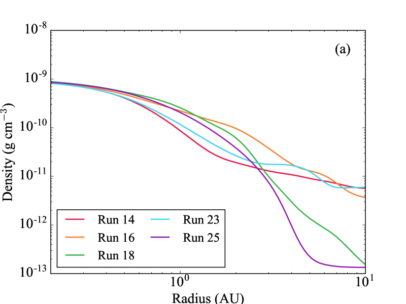
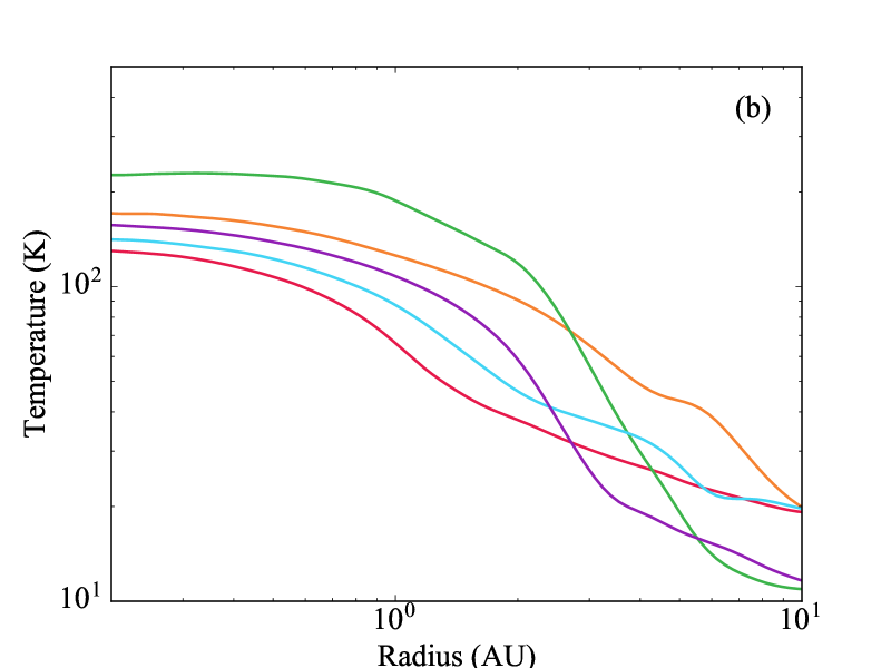
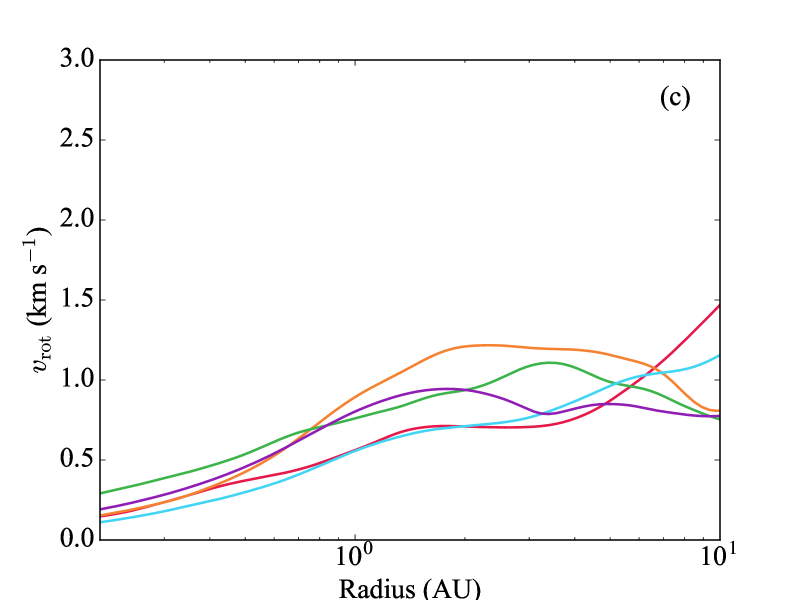
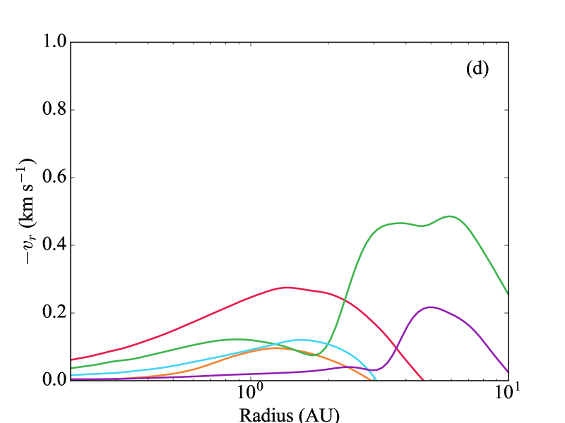
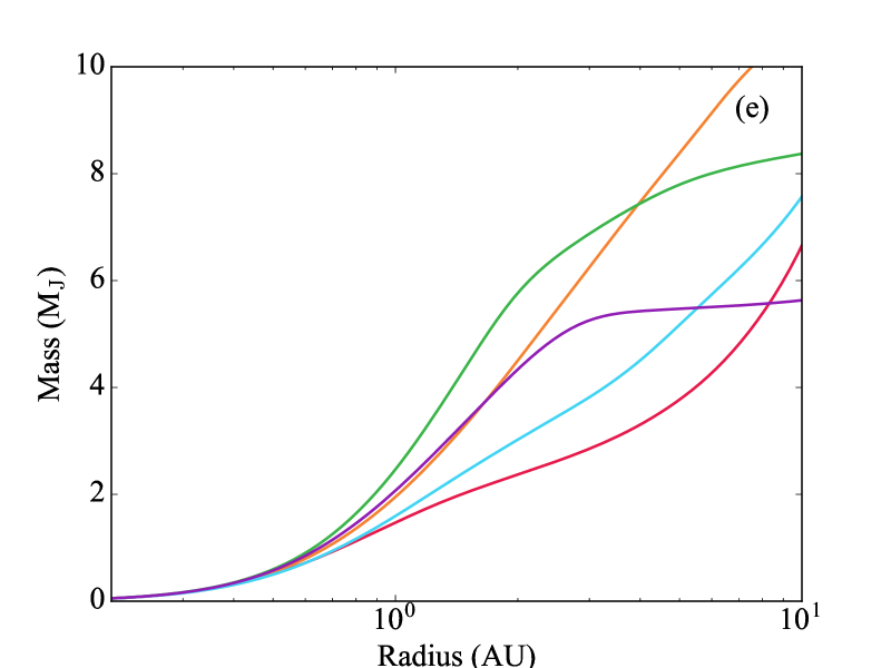
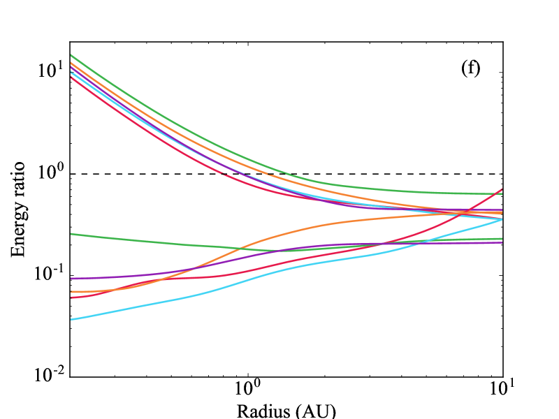
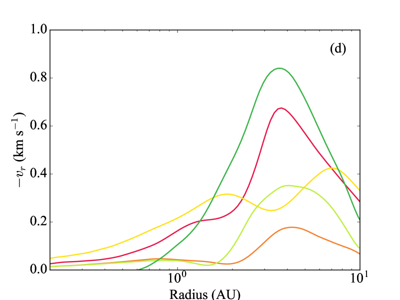
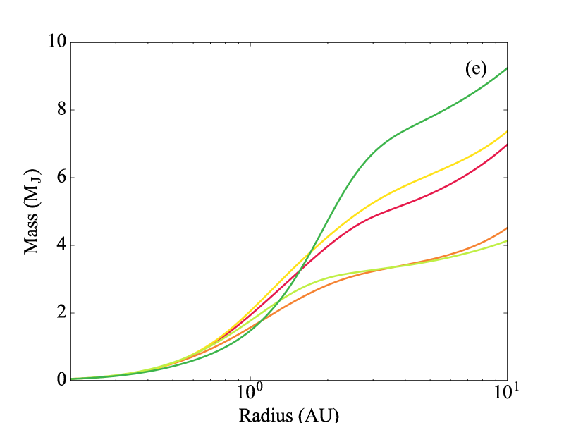
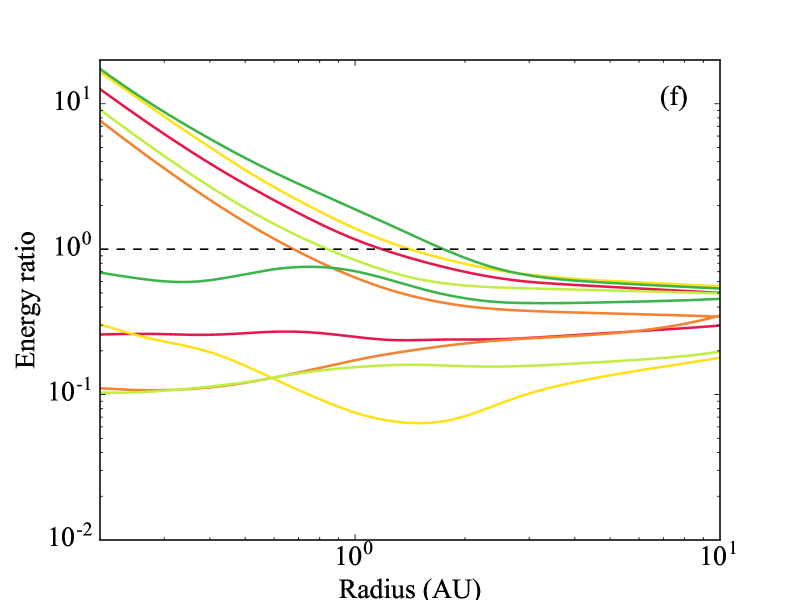
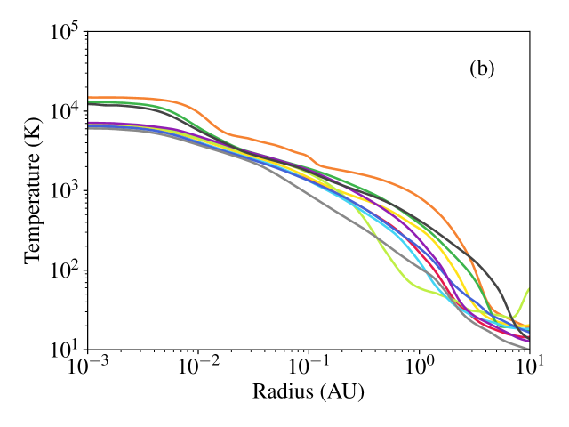
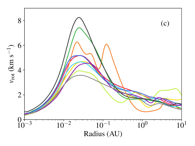
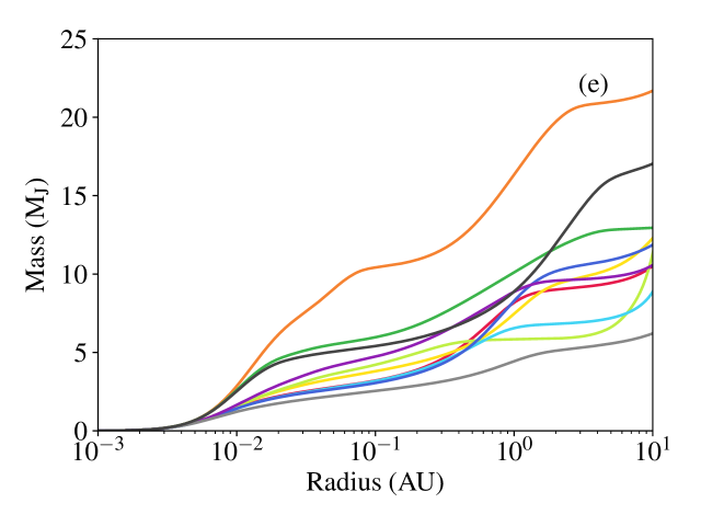
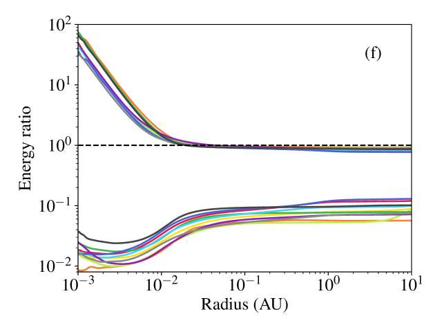
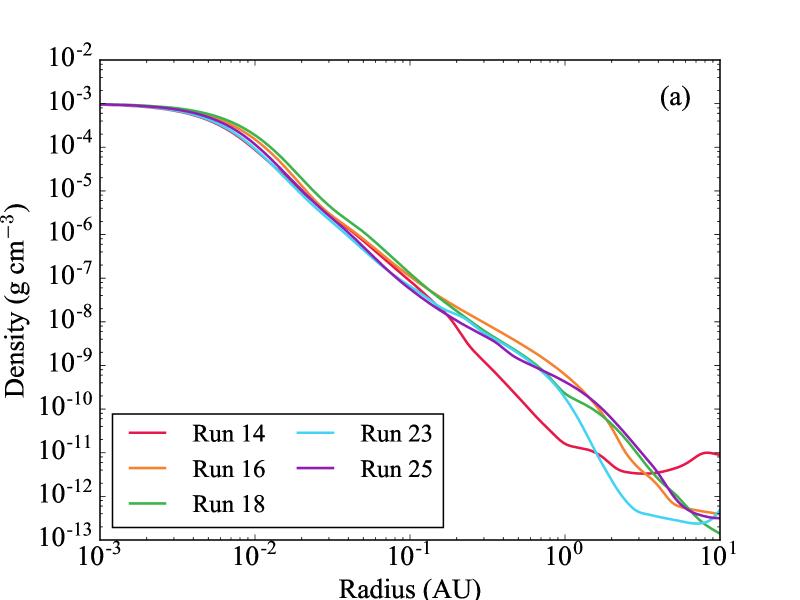
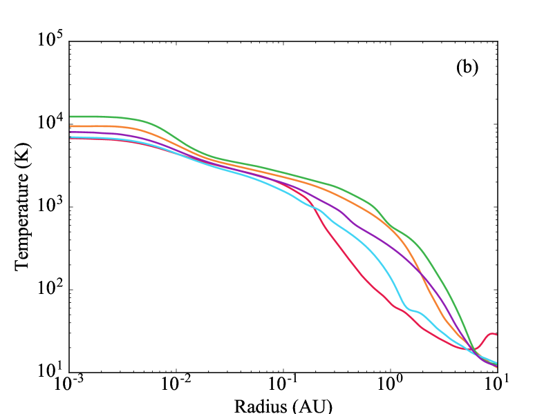
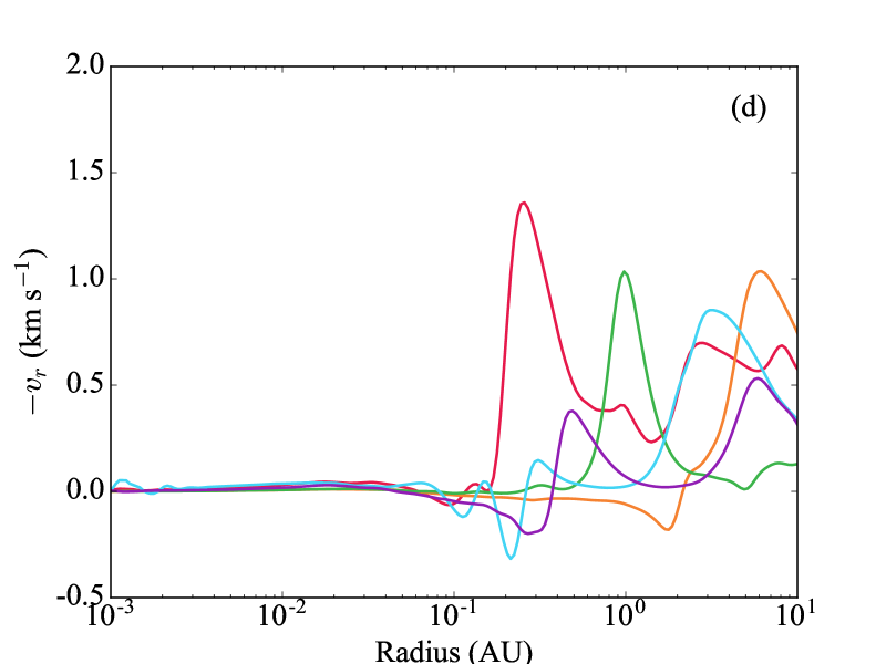
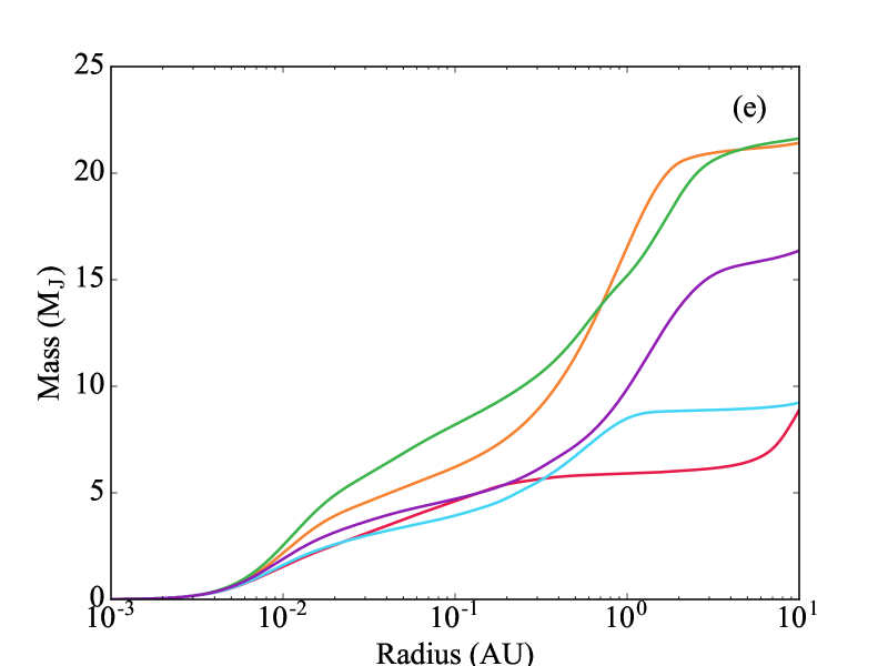
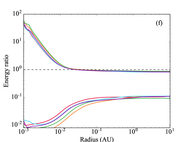
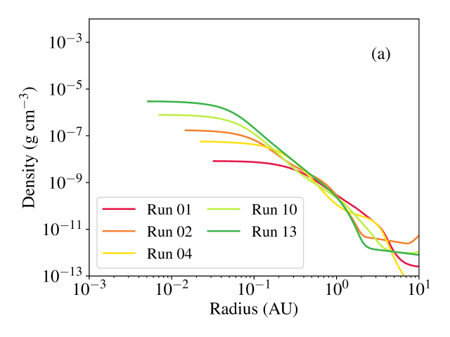
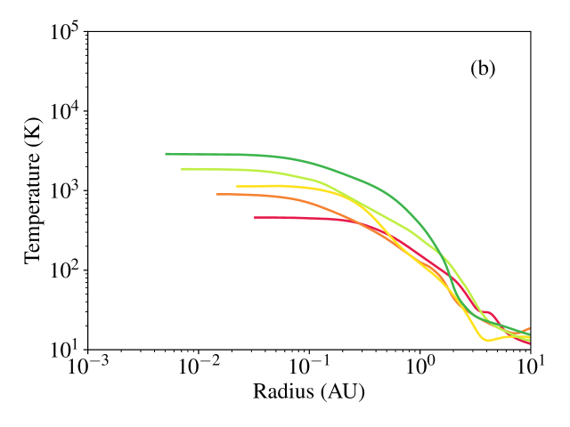
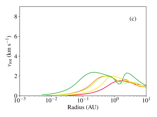
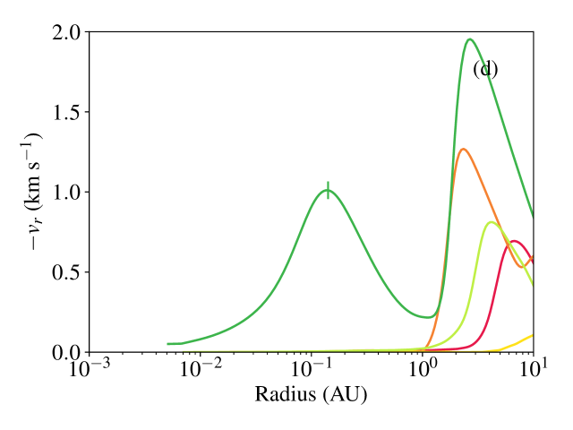
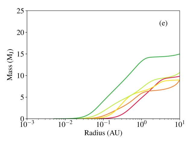
The evolution of the density, temperature, rotational velocity, infall velocity, mass, and ratios of the thermal-to-gravitational and rotational-to-gravitational energy as a typical fragment collapses (in Run 5) are shown in Figure 16. The fragment generally goes through the phase of first collapse, first core formation, second collapse, and second core formation (Stamatellos & Whitworth, 2009a), just like a solar-mass collapsing core (Larson, 1969; Masunaga et al., 1998; Masunaga & Inutsuka, 2000; Stamatellos et al., 2007b; Vaytet & Haugbølle, 2017; Bhandare et al., 2018). Initially, during the first collapse, the temperature increases slowly as the fragment is optically thin, but when it becomes optically thick the first hydrostatic core forms (as evidenced by the fragment infall velocity profile showing the accretion shock on the boundary of the first core) and the collapse slows down, proceeding quasi-statically and almost adiabatically. The temperature at the centre of the fragment eventually gets high enough ($\sim 2,000$ K) for molecular hydrogen to start dissociating, a process that acts as an energy sink. Then, the second collapse is initiated and the second core forms (as evidenced again by the accretion shock in the infall velocity profile).

(a)

(b)

(c)

(d)

(e)

(f)

Figure 16: Evolution of a representative protoplanet (Run 5). Panels (a) and (b) show the spherically-averaged density and temperature, respectively. Panels (c) and (d) show rotational (azimuthally-averaged) and radial infall velocity (spherically-averaged). The first and second hydrostatic cores boundaries are identified by the peaks in the infall velocity profiles (the positions of the boundaries are marked with the short vertical lines). Panel (e) shows the mass within a given radius within each fragment. Panel (f) shows the ratio of total energies interior to a given radius: $\alpha_{\rm therm}=E_{\textup{ther}}/E_{\textup{grav}}$ (top set of lines) and $\beta_{\rm rot}=E_{\textup{rot}}/E_{\textup{grav}}$ (bottom set of lines). The rotational energy is significant only in the outer parts of the fragment.

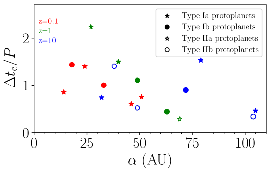
The simulations terminated once the density at the centre of the fragments reached $10^{-3}\textup{ g cm}^{-3}$ (although for a few of the simulations this density was not reached). We note however, that due to the rotation of the fragments and interactions with the disc and other fragments there were deviations from this general behaviour. We have therefore grouped the protoplanets that were formed in these simulations into 2 types (each with 2 sub-types).

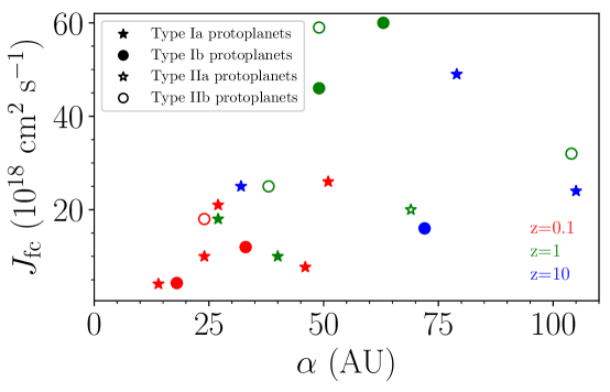
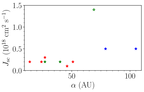
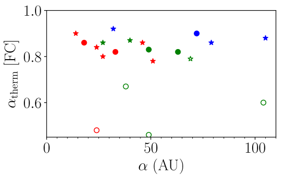
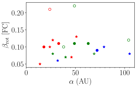
”Type I protoplanets” are defined as those protoplanets that undergo a second collapse (the temperature at their centre rises above $2,000$ K) reaching densities $10^{-3}\textup{ g cm}^{-3}$ at their centres. Most of these protoplanets (Type Ia protoplanets) have a second core as it evidenced by an accretion shock (seen in the infall velocity profile, Figure 16d). These protoplanets are depicted by filled stars in Figures 20-23. The radial profiles of their properties are shown in Figure 29. A few of these protoplanets (Type Ib protoplanets) show no signature of a second core in the infall velocity profiles. These are depicted by filled circles in Figures 20-23 and the radial profiles of their properties are shown in Figure 30.

”Type II protoplanets” are defined as those protoplanets that do not reach density $10^{-3}\textup{ g cm}^{-3}$ at their centres (at least for the time we follow their evolution). One of these protoplanets (Type IIa protoplanets; Run 13) undergoes a second collapse and shows evidence of a second core in the radial infall profile. This is depicted by an open star in Figures 20-23. However, the rest of these protoplanets do not undergo second collapse (Type IIb protoplanets). These are depicted by open circles in Figures 20-23. The radial profiles of the properties of Type II protoplanets are shown in Figure 31. It is expected that Type II protoplanets eventually evolve to Type I as more gas is accreted from the disc initiating the second collapse.

The properties of the protoplanets formed in the simulations are presented in Table 3. We define the boundaries of the first and second cores as the maxima in the infall velocity profiles. It is important to note that a few of the protoplanets (generally the ones that rotate faster) do not show clear velocity signatures of a second core (Type Ib; see discussion in Appendix A, Figure 32). In the table we also list the number of SPH particles within the first core, which is indicative of how well the first core is resolved. Generally, each first core is represented by more than $\sim 10^{5}$ SPH particles, which ensures that its collapse is well-resolved up to densities of $10^{-3}\textup{ g cm}^{-3}$ (see Stamatellos et al., 2007b). Due to computational constraints (the timestep becomes too short) we are unable to follow the evolution of the protoplanets after the second collapse. Previous studies (e.g. Stamatellos & Whitworth, 2009b) typically introduce sink particles to represent the protoplanets once they form. However, a more detailed treatment is required to accurately capture the internal evolution of these protoplanets as they interact with their parent disc in order to determine their final properties. Therefore, here we discuss only the initial properties of the protoplanets (i.e. when they form in the disc) and leave their subsequent evolution for a follow-up study.

Most of the protoplanets that form in the simulations presented here are Type I, that is, they have undergone second collapse and have reached central densities of $10^{-3}\textup{ g cm}^{-3}$. These protoplanets have reached high temperatures ($\sim 6,000-12,000\leavevmode\nobreak\$K; also seen in the lower-resolution simulations of Stamatellos & Whitworth (2009a)), and therefore correspond to the hot-start model of planet formation (e.g. Marley et al., 2007; Mordasini et al., 2012; Mordasini, 2013; Baruteau et al., 2016). The estimated temperatures are similar to the temperatures of the accretion shock around planets formed by core accretion (Marleau et al., 2017; Szulágyi, 2017; Szulágyi et al., 2018; Szulágyi & Mordasini, 2017; Marleau et al., 2019) and therefore their circumplanetary discs are also expected to be relatively hot. These high temperatures contradict the results of the disc instability model presented in Szulágyi et al. (2017), as in the simulations presented here we were able to follow the collapse of a fragment at much higher densities and capture the formation of the first and second core.

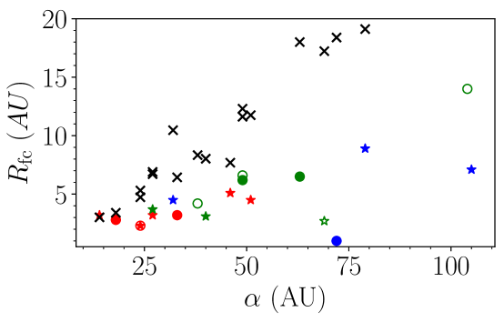
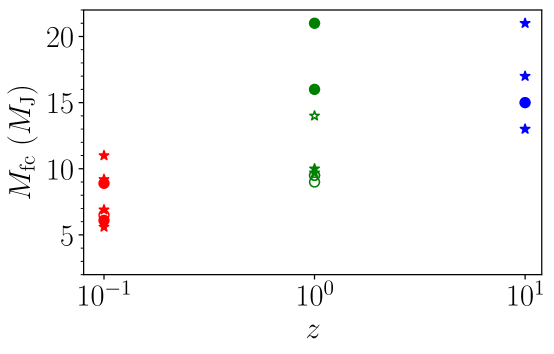
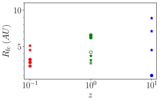
The first core masses are super-Jovian ($\stackrel{{\scriptstyle>}}{{{}_{\sim}}}5\textup{ M}_{\textsc{j}}$; see Figure 20), and in some cases, are higher (up to $20\textup{ M}_{\textsc{j}}$) than the deuterium burning mass limit of $\sim 13\textup{ M}_{\textsc{j}}$, that is, they are in the brown dwarf mass regime. They have radii between 1 and 10 AU, and in all cases their sizes are smaller than their corresponding Hill radii as expected (see Figure 20, black crosses on the left graph). The first cores form at distances from 15 to 100 AU, that is on relatively wide orbits. The masses and radii of the first cores tend to increase with metallicity (see Figure 20), although there is a rather considerable spread for each metallicity. This dependence is expected as at the high optical depth regime the cooling rate of the protoplanet decreases with increasing opacity and therefore the first core mass and radius increase (e.g. Masunaga et al., 1998; Masunaga & Inutsuka, 1999, 2000).

(a)

(b)

Figure 17: Mass (left) and radius (right) of the first cores formed in the simulations in Table 3. Different symbols correspond to different type of protoplanets (see discussion in text). Colours correspond to different opacities (red: $z=0.1$, green: $z=1$, blue: $z=10$). Black crosses correspond to the Hill radius of each fragment.

(a)

(b)

Figure 18: Mass (left) and radius (right) of the first cores versus metallicity $z$. Symbols are the same as in Figure 20.

(a)

(b)

Figure 19: Mass (left) and radius (right) of the second cores. Symbols and colours are the same as in Figure 20.

(a)

(b)

Figure 20: Mass (left) and radius (right) of the second cores versus metallicity $z$. Symbols and colours are the same as in Figure 20.

(a)

(b)

Figure 21: Specific angular momenta of the first (left) and second (right) cores of protoplanets formed by disc instability. Fragments that do not undergo a second collapse (open circles) tend to have higher specific angular momentum. Symbols are the same as in Figure 20.

(a)

(b)

(c)

(d)

Figure 22: Ratios of thermal-to-gravitational $\alpha_{\rm therm}={E_{\textup{ther}}}/{E_{\textup{grav}}}$ (left) and rotational-to-gravitational $\beta_{\rm rot}={E_{\textup{rot}}}/{E_{\textup{grav}}}$ (right), for the first (top) and second (bottom) cores. Fragments that do not undergo a second collapse (open circles) tend to have high fractions of rotational energy. Symbols are the same as in Figure 20.

Figure 23: Time (in units of the local orbital period, P) it takes for a protoplanet to collapse from $10^{-9}{\rm g\ cm}^{-3}$ to its final central density ($10^{-3}{\rm g\ cm}^{-3}$ for Type I protoplanets). Symbols are the same as in Figure 20.

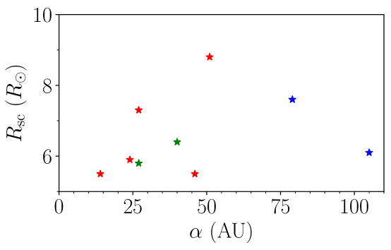
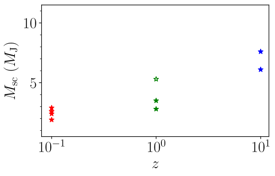
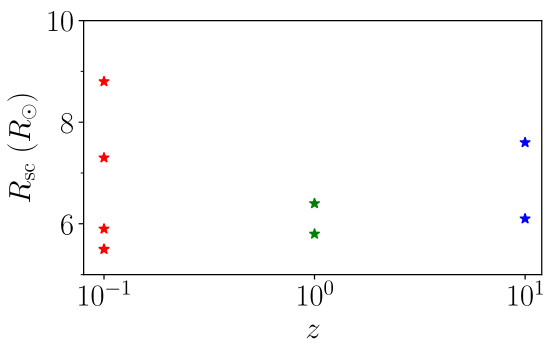
The second cores have masses of the order of a few Jupiter masses ($\sim 2-6\textup{ M}_{\textsc{j}}$; Figure 20, left) and radii of the order of a few solar radii ($\sim 5-9\;\textup{R}_{\odot}$; Figure 20, right). These masses and radii are similar to the ones of second cores formed in solar-mass collapsing cores (Larson, 1969; Masunaga & Inutsuka, 2000; Stamatellos et al., 2007b; Tomida et al., 2013; Vaytet et al., 2013; Bate, 2014; Tsukamoto et al., 2015; Bhandare et al., 2018). As with the first cores, the second core mass tends to be higher for higher metallicity, but there is no apparent relation between metallicity and the size of the second core (Figure 20).

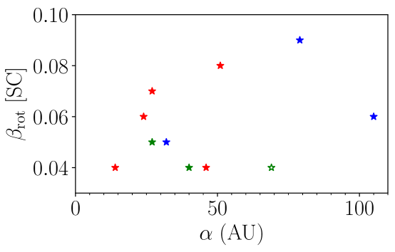
In Figure 23 we plot the specific angular momenta of the first and second cores, and in Figure 23 we plot the ratios of thermal-to-gravitational $\alpha_{\rm therm}={E_{\textup{ther}}}/{E_{\textup{grav}}}$ (left) and rotational-to-gravitational $\beta_{\rm rot}={E_{\textup{rot}}}/{E_{\textup{grav}}}$ (right), for the first (top) and second (bottom) cores. Fragments that do not undergo a second collapse (Type IIb protoplanets, open circles) or undergo a second collapse but without forming an accretion shock around the second core (Type Ia protoplanets, filled circles) tend to have high specific angular momentum and high rotational energy. This is similar to the behaviour of first and second cores forming in higher-mass (i.e. solar-mass) rotating cores (Saigo & Tomisaka, 2006; Saigo et al., 2008). However, we note that these graphs depict these properties at the final stage of the collapse. To determine the relation between fragment rotation and the presence or not of a second core, the pre-collapse properties of each fragment need to be examined and put in context with the movement of the fragment within the disc. We will investigate this issue in a subsequent paper.

The time it takes a protoplanet to collapse from a central density of $10^{-9}{\rm g\ cm}^{-3}$ to its final central density ($10^{-3}{\rm g\ cm}^{-3}$ for Type I protoplanets) is shown in Figure 23. It varies from 0.3 to 1.5 times the local orbital period which allows for possible interactions (and maybe disruption) before a bound second core forms.

7 Comparison with the observed properties of exoplanets around M dwarfs

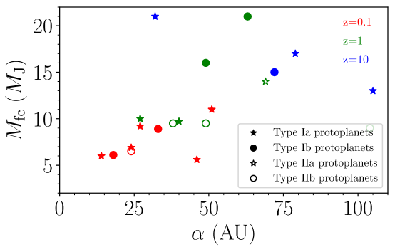
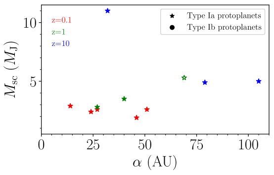
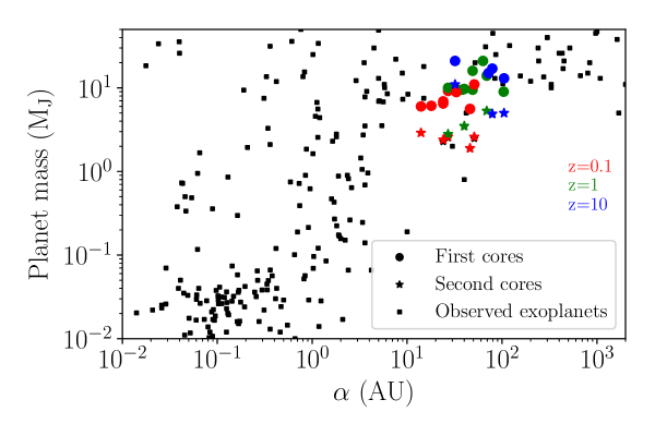
The initial masses of the protoplanets formed in our simulations by disc instability and their distances from their host star are shown in Figure 24, where they are compared against the properties of the observed exoplanets around M dwarfs. We plot the properties of both first and second cores. The disc instability exoplanets occupy the high-mass, wide-orbit region of the graph. Protoplanets formed through disc instability have super-Jovian masses ($2-5\textup{ M}_{\textsc{j}}$) and orbit at distances $10-100$ AU.

These protoplanet properties are expected to change due to interactions with the disc and with other protoplanets (Forgan & Rice, 2013; Nayakshin, 2017a, b; Hall et al., 2017; Forgan et al., 2018; Stamatellos & Inutsuka, 2018; Fletcher et al., 2019). Protoplanets may migrate inwards rapidly until they open up a gap (Stamatellos, 2015; Stamatellos & Inutsuka, 2018). Thereafter they may continue to migrate inwards slowly or start migrating outward s, if the edges of the gap within which the planet resides are gravitationally unstable. Additionally, stochastic migration of young protoplanets may happen due to gravitational interactions with other protoplanets in the disc (e.g. Veras & Raymond, 2012). The protoplanet mass may also increase significantly as they can accrete gas from the relatively massive disc (Stamatellos & Inutsuka, 2018). This could increase the protoplanet’s mass so that it may become a brown dwarf ($M>13\textup{ M}_{\textsc{j}}$) or a hydrogen-burning star ($M>80\textup{ M}_{\textsc{j}}$) (Stamatellos & Whitworth, 2009b; Kratter et al., 2010; Zhu et al., 2012). The gas accretion rate onto the protoplanet can be reduced if the planet is hot enough to heat the neighbouring disc (e.g. Stamatellos & Inutsuka, 2018; Mercer & Stamatellos, 2017). Alternatively, a protoplanet may undergo tidal downsizing, that is, tidal stripping via disruption from another protoplanet or during migration, reducing its mass even potentially in the terrestrial mass regime (Nayakshin, 2010, 2011; Humphries et al., 2019; Humphries & Nayakshin, 2019). More studies are needed to determine the final properties of protoplanets formed by disc instability (Müller et al., 2018), taking into account computational issues (Fletcher et al., 2019).

Figure 24: Masses ($M_{p}\sin(i)$, where $i$ is the planet orbit orientation) of planets around M dwarfs ($M_{\star}<0.5\textup{ M}_{\odot}$) as a function of their semi-major axis. Black points correspond to the observed exoplanets. The coloured symbols correspond to the protoplanets formed in the simulations presented here. Circles correspond to first cores, whereas stars to the second cores. Colours correspond to different opacities (red: $z=0.1$, green: $z=1$, blue: $z=10$). As these protoplanets are still embedded within their protostellar discs, they may migrate inwards or outwards, changing their final semi-major axis. Similarly, they may undergo gas accretion or tidal stripping, changing their final mass.

8 Conclusions

We have performed a set of hydrodynamic simulations of protostellar discs around M dwarf stars. We varied the initial stellar mass such that $M_{\star}=[0.2,0.3,0.4]\textup{ M}_{\odot}$, as well as the initial disc radius, $R_{\textup{out}}=[60,90,120]$ AU. Additionally, we investigated the effect of metallicity, $z=[0.1,1,10]$. The discs that we studied were initially stable, but their masses were steadily increased through the method of mass loading, which can be notionally thought as accretion from an envelope during the early stage of star and disc formation. Most of the discs eventually became gravitationally unstable, spiral arms developed, and in the majority of cases, a protoplanet formed via fragmentation. The formation of protoplanets happens fast on a dynamical timescale (within 30 kyr). The density requirement for fragment formation was chosen to be $\rho>10^{-9}\textup{ g cm}^{-3}$ that is, a threshold typically reached during gravitational collapse after the formation of the first hydrostatic core (Larson, 1969). From the simulations of discs that do fragment, we determined the minimum disc mass necessary for fragmentation to occur and the properties of the resulting protoplanets.

The fragmentation of protostellar discs around M dwarfs requires a disc-to-star mass ratio of at least $q\sim 0.3$ for smaller discs, increasing to $q\sim 0.6$ for larger discs. These mass ratios are relatively high. However, there are observed systems with planet-to-star mass ratio of $\sim 0.2$ (see the exoplanet.eu database at https://exoplanet.eu), which confirms that the discs in which they have formed must have had at least 20% the mass of their host stars. In fact this fraction could have been much higher, considering that there may be other planets in the system not yet detected and that a significant fraction of the disc mass is lost due to accretion onto the central star and due to disc winds.

The mass at which a disc fragments increases with the size of the disc and the mass of the central star. However, no fragmentation occurs for small discs (initial radius $R_{\textup{init}}=60$ AU) around more massive M dwarfs (mass $0.4\textup{ M}_{\odot}$). This is likely due to rapid disc expansion because of the formation of strong spiral features, combined with stronger rotational support to the smaller disc and inefficient cooling closer to the central star. This is in agreement with previous analytical (Whitworth & Stamatellos, 2006) and numerical (e.g. Stamatellos & Whitworth, 2009b; Mercer et al., 2018) studies that show that fragmentation can happen only in the outer regions of extended discs. We find that the optimal region for fragmentation around M dwarfs is around 50 AU, that is, closer to the host star than what expected for higher mass (e.g. solar-type) stars (e.g. Stamatellos & Whitworth, 2009b). We find that the small discs (but still with size $>75$ AU) around lower mass M dwarfs are most susceptible to gravitational fragmentation.

The disc metallicity does not significantly affect the mass at which a disc fragments, but in some cases fragmentation may be suppressed. In the cases where the metallicity is an order of magnitude smaller, spiral arms take more time to fragment. When the metallicity is increased by an order of magnitude, spiral arms take longer to develop, and the disc may not undergo gravitational fragmentation at all due to a period of rapid expansion combined with inefficient cooling.

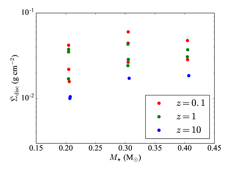
To facilitate comparisons with disc observations, we have calculated the average surface density $\bar{\Sigma}_{\textup{disc}}$ for the discs that fragment for a variety of stellar masses, shown in Figure 25. We find that disc fragmentation requires an average surface density $\bar{\Sigma}_{\textup{disc}}>0.01\textup{ g cm}^{-2}$ and that higher metallicity discs can fragment at a lower average density (although small-sized, high-metallicity discs may not fragment due to a period of rapid expansion). We note however that the minimum surface density needed for fragmentation does not increase monotonically with the metallicity (at least for the parameter space investigated in this paper).

Figure 25: Average surface density of the discs at the time they fragment where, $\bar{\Sigma}_{\textup{disc}}=M_{\textup{disc}}/\pi R_{\textup{disc}}^{2}$. We find that a lower average surface density is required for fragmentation when the disc metallicity is higher.

Protoplanets due to disc instability around M dwarfs form very fast, on a dynamical timescale (within a few thousand years). Initially they are massive ($2-6\textup{ M}_{\textsc{j}}$) and on wide orbits ($15-105$ AU). Those that form in high metallicity discs are more massive and form on initially wider orbits. However, both masses and orbital radii are expected to evolve as the protoplanets interact with their discs; therefore, their long term evolution must be studied in order to compare these with the corresponding properties of the observed exoplanets around M dwarfs. All protoplanets formed in the simulations presented in this paper have similar density and temperature profiles, and possess significant rotational energy, which in some cases may delay or even suppress the second collapse of the protoplanet. Nevertheless, most of the exoplanets undergo the second collapse phase and therefore attain high central temperatures (6,000-12,000 K). These temperatures are similar to the temperatures at the accretion shocks around planets formed by core accretion (Szulágyi et al., 2017; Marleau et al., 2019), therefore the temperature alone cannot provide a way to distinguish between these two formation scenarios.

We conclude that disc instability may be a viable way to quickly form gas giant planets on wide orbits around M dwarfs that are difficult to form by core accretion, provided that discs around M dwarfs have significant mass when compared to the mass of their host star. Future observations of massive young discs embedded in their parental clouds or of planets that have formed fast around very young proto- M dwarfs could provide evidence that disc instability occurs. Wide orbit planets formed in this way may migrate inwards or outwards, contributing to the observed population of planets around M dwarfs at various orbital radii.

Appendix A Fragment and protoplanet properties

We present plots of the properties of all fragments and protoplanets formed in the simulations we have performed, as these correspond to the initial stages of disc instability planets and therefore need to be further investigated.

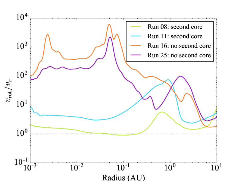
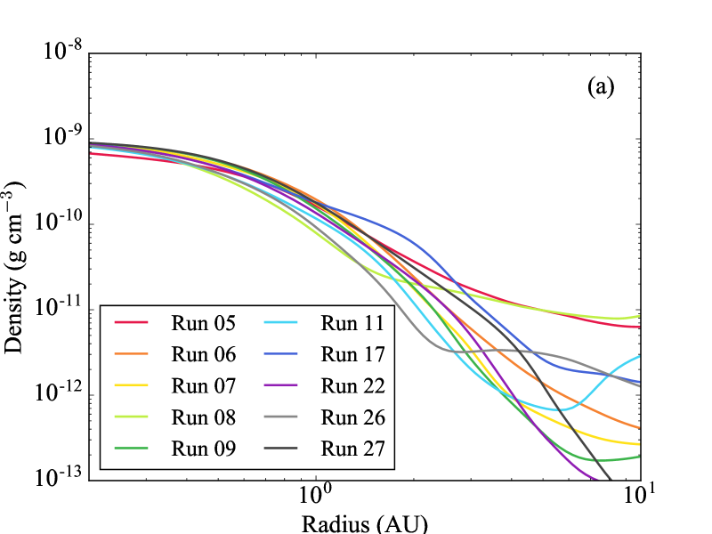
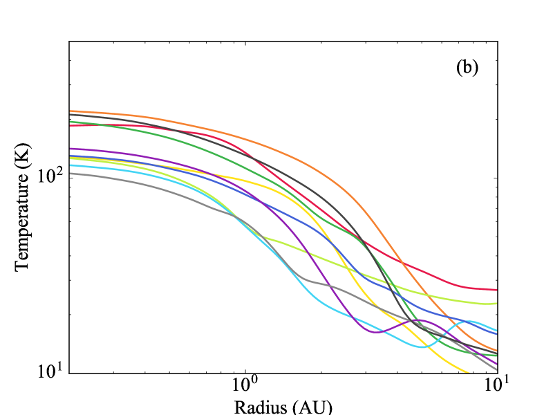
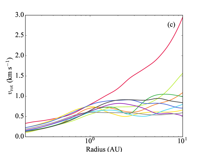
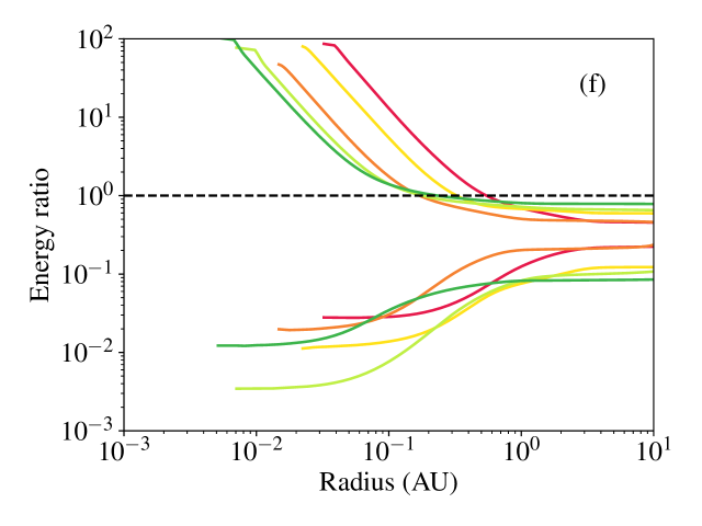
Plots of the radial profiles of various properties for all fragments at central density $10^{-9}{\rm g\ cm}^{-3}$ (Figures 26-28), and protoplanets (Type I and II, see discussion in Section 6) (Figures 29-31) are presented. Structurally, protoplanets are similar to one another, differing only in mass. The temperature is generally higher within the more massive protoplanets. The rotational velocity is comparable to the infall velocity but despite this, the ratio between rotational energy and gravitational energy is generally small throughout, between 0.01 and 0.1. The thermal energy is comparable to the gravitational energy.

(a)

(b)

(c)

(d)

(e)

(f)

Figure 26: Properties of a set of fragments when they have attained a central density of $10^{-9}\textup{ g cm}^{-3}$. Panels are the same as in Figure 16. The thermal-to-gravitational energy ratios are comparable for different fragments. Rotational energy is significant only in the outer parts of each fragment.

(a)

(b)

(c)

(d)

(e)

(f)

Figure 27: Properties of a set of fragments formed in the simulations (same as in Figure 26, but for a different set of fragments).

(a)

(b)

(c)

(d)

(e)

(f)

Figure 28: Properties of a set of fragments formed in the simulations (same as in Figure 26, but for a different set of fragments).

(a)

(b)

(c)

(d)

(e)

(f)

Figure 29: Properties of Type Ia protoplanets, that is, fragments which have undergone second collapse and attained a central density of $10^{-3}\textup{ g cm}^{-3}$. Panels (a) and (b) show the spherically-averaged density and temperature, respectively. They do not vary significantly from protoplanet to protoplanet, though the protoplanets in runs 6, 9 and 27 posses denser and hotter central regions due to their higher mass. Panels (c) and (d) show rotational (azimuthally-averaged) and infall velocity (spherically-averaged), the former of which is significant as the protoplanets reside in a rotating disc. The peaks in infall velocity are indicative boundaries where gas begins to decelerate. The second core boundaries are at $R=10^{-2}-10^{-1}$ AU and the first core boundaries at $R=1-10$ AU. Panel (e) shows the mass of the protoplanet within a given radius, demonstrating that even in low mass discs, the mass of formed objects is of the order of a few $\textup{M}_{\textsc{j}}$ or higher. Panel (f) shows the ratio of energies interior to a given radius: $E_{\textup{ther}}/E_{\textup{grav}}$ (top set of lines) and $E_{\textup{rot}}/E_{\textup{grav}}$ (bottom set of lines). Rotational energy is generally much lower than the gravitational energy. The short vertical lines in (d) indicate the positions of the second cores.

(a)

(b)

(c)

(d)

(e)

(f)

Figure 30: Properties of Type Ib protoplanets formed in the simulations (same as in Figure 29). The protoplanets presented here are the fragments that have undergone second collapse but do not show any infall velocity signatures indicative of a second core. They are structurally similar to the Type Ia protoplanets in Figure 29, however the infall velocities here are almost zero or slightly negative, that is, indicative of a slowly-expanding protoplanet core.

(a)

(b)

(c)

(d)

(e)

(f)

Figure 31: Properties of Type II protoplanets formed in the simulations (same as in Figure 29, that is, fragments that do not reach a density of $10^{-3}\textup{ g cm}^{-3}$ at their centres). One of these protoplanets (Type IIa; Run 13) undergoes a second collapse and shows evidence of a second core in the radial infall profile. This is depicted by open stars in Figures. However, most of these protoplanets do not undergo second collapse (Type IIb). The short vertical line in (d) indicates the position of the second core for Run 13.

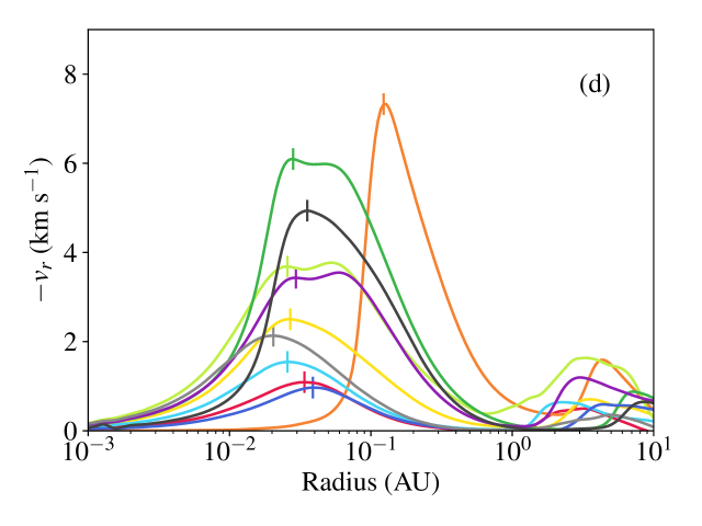
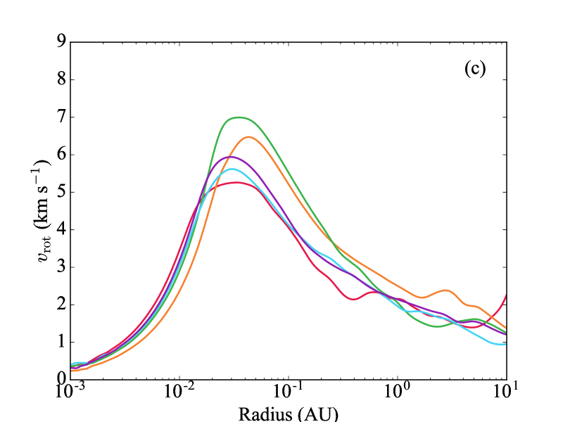
A few of the protoplanets formed in the simulations do not show clear signs of a second core (Type Ib protoplanets), despite having undergone a second collapse (see Figure 30 and Figure 31). These protoplanets have almost zero infall velocities (or slightly negative in some cases, indicative of a slow expansion) and they seem to be fast rotating. Figure 32 shows azimuthally-averaged radial profiles of the ratio between rotational to infall velocity. We compare protoplanets which show a clear sign of second core formation with those that do not. The protoplanets with a second core (Type Ia, IIa; runs 8 and 11, green and blue lines, respectively) have $v_{\textup{rot}}/v_{r}<10$ in their inner regions, which is relatively low compared to the protoplanets without second cores (Type Ib, IIb; $v_{\textup{rot}}/v_{r}>10^{2}$). In these latter cases (runs 16 and 25, orange and purple lines, respectively), the rotational velocity is a factor of 2 - 4 magnitudes higher than the infall velocity.

Figure 32: Ratio of the azimuthally-averaged rotational-to-infall velocity for a set of protoplanets with and without any second core signatures as determined from infall velocity peaks. The protoplanets in Runs 8 and 11 (Type Ia protoplanets) show signs of second cores in their infall velocities and exhibit values of $v_{\textup{rot}}/v_{r}<10$ in their inner regions. The protoplanets in Runs 16 and 25 (Type Ib protoplanets) do not show second core signatures, and their rotational velocity is of the order of 3 magnitudes higher than the infall velocity in their inner regions. The significant amount of rotation inhibits the formation of an accretion shock around the second core.