Adaptive Teaching of Temporal Logic Formulas to Learners with Preferences

Zhe Xu, Yuxin Chen, and Ufuk Topcu Zhe Xu is with the Oden Institute for Computational Engineering and Sciences, University of Texas, Austin, Austin, TX 78712, Yuxin Chen is with the Department of Computer Science, University of Chicago, Chicago, IL 60637, Ufuk Topcu is with the Department of Aerospace Engineering and Engineering Mechanics, and the Oden Institute for Computational Engineering and Sciences, University of Texas, Austin, Austin, TX 78712, e-mail: zhexu@utexas.edu, chenyuxin@uchicago.edu, utopcu@utexas.edu.
Abstract

Machine teaching is an algorithmic framework for teaching a target hypothesis via a sequence of examples or demonstrations. We investigate machine teaching for temporal logic formulas—a novel and expressive hypothesis class amenable to time-related task specifications. In the context of teaching temporal logic formulas, an exhaustive search even for a myopic solution takes exponential time (with respect to the time span of the task). We propose an efficient approach for teaching parametric linear temporal logic formulas. Concretely, we derive a necessary condition for the minimal time length of a demonstration to eliminate a set of hypotheses. Utilizing this condition, we propose a myopic teaching algorithm by solving a sequence of integer programming problems. We further show that, under two notions of teaching complexity, the proposed algorithm has near-optimal performance. The results strictly generalize the previous results on teaching preference-based version space learners. We evaluate our algorithm extensively under a variety of learner types (i.e., learners with different preference models) and interactive protocols (e.g., batched and adaptive). The results show that the proposed algorithms can efficiently teach a given target temporal logic formula under various settings, and that there are significant gains of teaching efficacy when the teacher adapts to the learner’s current hypotheses or uses oracles.

1 Introduction

Machine teaching, also known as algorithmic teaching, is an algorithmic framework for teaching a target hypothesis via a sequence of examples or demonstrations [1]. Due to limited availability of data or high cost of data collection in real-world learning scenarios, machine teaching provides a viable solution to optimize the training data for a learner to efficiently learn a target hypothesis.

Recently, there has been an increasing interest in designing learning algorithms for inferring task specifications from data (e.g., in robotics) [2, 3]. Machine teaching can be used to optimize the training data for various learning algorithms [4], hence it can be potentially used for task specification inference algorithms. Machine teaching can be also used in adversarial settings [5] where an attacker (machine teaching algorithm) manipulates specification inference by modifying the training data. Unfortunately, finding the optimal teaching sequence with minimal teaching cost is notoriously hard [6]. As task specifications are often time-related and the demonstration data are trajectories with a time evolution, an exhaustive search even for the myopic solution has exponential time complexity with the time span of the task, making it prohibitive to run existing myopic teaching algorithms in practice.

In this paper, we investigate machine teaching of target hypothesis represented in temporal logic [7], which has been used to express task specifications in many applications in robotics and artificial intelligence [8, 9]. Specifically, we use a fragment of parametric linear temporal logic (pLTL) [10, 11]. We derive a necessary condition for the minimal time length of a demonstration so that a set of pLTL formulas can be eliminated by this demonstration. Utilizing this necessary condition, we provide a myopic teaching approach by solving a sequence of integer programming problems which, under certain conditions, guarantees a logarithmic factor of the optimal teaching cost.

We evaluate the proposed algorithm extensively under a variety of learner types (i.e., learner with different preference models) and interactive protocols (i.e., batched and adaptive). The results show that the proposed algorithm can efficiently teach a given target hypothesis under various settings, and that there are significant gains of teaching efficacy when the teacher adapts to the learner’s current hypotheses (up to 31.15% reduction in teaching cost compared to the non-adaptive setting) or with oracles (up to 75% reduction in teaching cost compared to the myopic setting).

Related Work

There has been a surge of interest in machine teaching in several different application domains, including personalized educational systems [1], citizen sciences [12], adversarial attacks [5] and imitation learning [13]. Most theoretical work in algorithmic machine teaching assumes the version space model [6, 14, 15, 16]. Recently, some teaching complexity results have been extended beyond version space learners, such as Bayesian learners [17] and gradient learners [18] (e.g., learners implementing a gradient-based optimization algorithm). However, most algorithms are restricted to simple concept classes. In this work, we aim to understand the complexity of teaching the class of pLTL formulas. There has been extensive study in modeling a learner for temporal logic formulas, for example, see [19, 2, 20, 21, 3, 22, 23, 24, 25, 26, 27, 28], while it is much less understood in the context of machine teaching. In this paper, we abstract these learner models as preference-based version space learners, and focus on developing efficient algorithms for teaching such learners.

2 Parametric Linear Temporal Logic

In this section, we present an overview of parametric linear temporal logic (pLTL) [10, 11]. We start with the syntax and semantics of pLTL. The domain 𝔹={,}𝔹topbottom\mathbb{B}=\{\top,\bot\} (top\top and bottom\bot represents True and False respectively) is the Boolean domain and the time index set 𝕋={0,1,}𝕋01\mathbb{T}=\{0,1,\dots\} is a discrete set of natural numbers. We assume that there is an underlying system \mathcal{H}. The state s𝑠s of the system \mathcal{H} belongs to a finite set S𝑆S of states. A trajectory ρL=s0s1sL1subscript𝜌𝐿subscript𝑠0subscript𝑠1subscript𝑠𝐿1\rho_{L}=s_{0}s_{1}\cdots s_{L-1} of length L>0𝐿subscriptabsent0L\in\mathbb{Z}_{>0} describing an evolution of the system \mathcal{H} is a function from 𝕋𝕋\mathbb{T} to S𝑆S. A set 𝒜𝒫={π1,π2,,πn}𝒜𝒫subscript𝜋1subscript𝜋2subscript𝜋𝑛\mathcal{AP}=\{\pi_{1},\pi_{2},\dots,\pi_{n}\} is a set of atomic predicates. :S2𝒜𝒫:𝑆superscript2𝒜𝒫\mathcal{L}:S\rightarrow 2^{\mathcal{AP}} is a labeling function assigning a subset of atomic predicates in 𝒜𝒫𝒜𝒫\mathcal{AP} to each state sS𝑠𝑆s\in S. The syntax of the (F,G)-fragment bounded pLTL is defined recursively as111Although other temporal operators such as “Until ”(𝒰𝒰\mathcal{U}) may also appear in the full syntax of pLTL, they are omitted from the syntax of (F,G)-fragment bounded pLTL as they can be hard to interpret and are not often used for the inference of pLTL formulas.

ϕ:=π¬ϕϕ1ϕ2GτϕFτϕ,assignitalic-ϕtopconditionaldelimited-∣∣𝜋italic-ϕdelimited-∣∣subscriptitalic-ϕ1subscriptitalic-ϕ2subscript𝐺absent𝜏italic-ϕsubscript𝐹absent𝜏italic-ϕ\begin{split}\phi:=&\top\mid\pi\mid\lnot\phi\mid\phi_{1}\wedge\phi_{2}\mid G_{\leq\tau}\phi\mid F_{\leq\tau}\phi,\end{split}

where π𝜋\pi is an atomic predicate; ¬\lnot and \wedge stand for negation and conjunction, respectively; Gτsubscript𝐺absent𝜏G_{\leq\tau} and Fτsubscript𝐹absent𝜏F_{\leq\tau} are temporal operators representing “parameterized always” and “parameterized eventually”, respectively (τ𝕋𝜏𝕋\tau\in\mathbb{T} is a temporal parameter). From the above-mentioned operators, we can also derive other operators such as \vee (disjunction) and \Rightarrow (implication). In the following content of the paper, we refer to (F,G)-fragment bounded pLTL as pLTLf for brevity.

Next, we introduce the Boolean semantics of a pLTLf formula in the strong and the weak view [29, 30, 31]. In the following, (ρL,t)SϕsubscriptmodelsSsubscript𝜌𝐿𝑡italic-ϕ(\rho_{L},t)\models_{\rm{S}}\phi (resp. (ρL,t)WϕsubscriptmodelsWsubscript𝜌𝐿𝑡italic-ϕ(\rho_{L},t)\models_{\rm{W}}\phi) means the trajectory ρLsubscript𝜌𝐿\rho_{L} strongly (resp. weakly) satisfies ϕitalic-ϕ\phi at time t𝑡t, and (ρL,t)⊧̸Sϕsubscriptnot-modelsSsubscript𝜌𝐿𝑡italic-ϕ(\rho_{L},t)\not\models_{\rm{S}}\phi (resp. (ρL,t)⊧̸Wϕsubscriptnot-modelsWsubscript𝜌𝐿𝑡italic-ϕ(\rho_{L},t)\not\models_{\rm{W}}\phi) means the trajectory ρLsubscript𝜌𝐿\rho_{L} fails to strongly (resp. weakly) satisfy ϕitalic-ϕ\phi at time t𝑡t.

Definition 1.

The Boolean semantics of the pLTLf in the strong view is defined recursively as

(ρL,t)SπifftL1andf(ρL(t))>0,(ρL,t)S¬ϕiff(ρL,t)⊧̸Wϕ,(ρL,t)Sϕ1ϕ2iff(ρL,t)Sϕ1and(ρL,t)Sϕ2,(ρL,t)SFτϕifft[t,t+τ],s.t.(ρL,t)Sϕ,(ρL,t)SGτϕiff(ρL,t)Sϕ,t[t,t+τ].formulae-sequenceformulae-sequencesubscriptmodelsSsubscript𝜌𝐿𝑡𝜋iff𝑡𝐿1and𝑓subscript𝜌𝐿𝑡0formulae-sequencesubscriptmodelsSsubscript𝜌𝐿𝑡italic-ϕformulae-sequencesubscriptnot-modelsWiffsubscript𝜌𝐿𝑡italic-ϕformulae-sequencesubscriptmodelsSsubscript𝜌𝐿𝑡subscriptitalic-ϕ1subscriptitalic-ϕ2subscriptmodelsSiffsubscript𝜌𝐿𝑡subscriptitalic-ϕ1andsubscript𝜌𝐿𝑡subscriptmodelsSsubscriptitalic-ϕ2formulae-sequencesubscriptmodelsSsubscript𝜌𝐿𝑡subscript𝐹absent𝜏italic-ϕiffsuperscript𝑡𝑡𝑡𝜏𝑠𝑡formulae-sequencesubscriptmodelsSsubscript𝜌𝐿superscript𝑡italic-ϕformulae-sequencesubscriptmodelsSsubscript𝜌𝐿𝑡subscript𝐺absent𝜏italic-ϕformulae-sequencesubscriptmodelsSiffsubscript𝜌𝐿superscript𝑡italic-ϕfor-allsuperscript𝑡𝑡𝑡𝜏\begin{split}(\rho_{L},t)\models_{\rm{S}}\pi\quad\mbox{iff}\quad&t\leq L-1~{}\mbox{and}~{}f(\rho_{L}(t))>0,\\ (\rho_{L},t)\models_{\rm{S}}\lnot\phi\quad\mbox{iff}\quad&(\rho_{L},t)\not\models_{\rm{W}}\phi,\\ (\rho_{L},t)\models_{\rm{S}}\phi_{1}\wedge\phi_{2}\quad\mbox{iff}\quad&(\rho_{L},t)\models_{\rm{S}}\phi_{1}~{}\mbox{and}~{}(\rho_{L},t)\models_{\rm{S}}\phi_{2},\\ (\rho_{L},t)\models_{\rm{S}}F_{\leq\tau}\phi\quad\mbox{iff}\quad&\exists t^{\prime}\in[t,t+\tau],s.t.~{}(\rho_{L},t^{\prime})\models_{\rm{S}}\phi,\\ (\rho_{L},t)\models_{\rm{S}}G_{\leq\tau}\phi\quad\mbox{iff}\quad&(\rho_{L},t^{\prime})\models_{\rm{S}}\phi,\forall t^{\prime}\in[t,t+\tau].\end{split}
Definition 2.

The Boolean semantics of the pLTLf in the weak view is defined recursively as
(ρL,t)Wπiffeithert>L1,or(tL1andf(ρL(t))>0),(ρL,t)W¬ϕiff(ρL,t)⊧̸Sϕ,(ρL,t)Wϕ1ϕ2iff(ρL,t)Wϕ1and(ρL,t)Wϕ2,(ρL,t)WFτϕifft[t,t+τ],s.t.(ρL,t)Wϕ,(ρL,t)WGτϕiff(ρL,t)Wϕ,t[t,t+τ].formulae-sequenceformulae-sequencesubscriptmodelsWsubscript𝜌𝐿𝑡𝜋formulae-sequenceiffeither𝑡𝐿1or𝑡𝐿1and𝑓subscript𝜌𝐿𝑡0formulae-sequencesubscriptmodelsWsubscript𝜌𝐿𝑡italic-ϕformulae-sequencesubscriptnot-modelsSiffsubscript𝜌𝐿𝑡italic-ϕformulae-sequencesubscriptmodelsWsubscript𝜌𝐿𝑡subscriptitalic-ϕ1subscriptitalic-ϕ2subscriptmodelsWiffsubscript𝜌𝐿𝑡subscriptitalic-ϕ1andsubscript𝜌𝐿𝑡subscriptmodelsWsubscriptitalic-ϕ2formulae-sequencesubscriptmodelsWsubscript𝜌𝐿𝑡subscript𝐹absent𝜏italic-ϕiffsuperscript𝑡𝑡𝑡𝜏𝑠𝑡formulae-sequencesubscriptmodelsWsubscript𝜌𝐿superscript𝑡italic-ϕformulae-sequencesubscriptmodelsWsubscript𝜌𝐿𝑡subscript𝐺absent𝜏italic-ϕformulae-sequencesubscriptmodelsWiffsubscript𝜌𝐿superscript𝑡italic-ϕfor-allsuperscript𝑡𝑡𝑡𝜏\begin{split}(\rho_{L},t)\models_{\rm{W}}\pi\quad\mbox{iff}\quad&\textrm{either}~{}t>L-1,\\ &\mbox{or}~{}\big{(}t\leq L-1~{}\mbox{and}~{}f(\rho_{L}(t))>0\big{)},\\ (\rho_{L},t)\models_{\rm{W}}\lnot\phi\quad\mbox{iff}\quad&(\rho_{L},t)\not\models_{\rm{S}}\phi,\\ (\rho_{L},t)\models_{\rm{W}}\phi_{1}\wedge\phi_{2}\quad\mbox{iff}\quad&(\rho_{L},t)\models_{\rm{W}}\phi_{1}~{}\mbox{and}~{}(\rho_{L},t)\models_{\rm{W}}\phi_{2},\\ (\rho_{L},t)\models_{\rm{W}}F_{\leq\tau}\phi\quad\mbox{iff}\quad&\exists t^{\prime}\in[t,t+\tau],s.t.~{}(\rho_{L},t^{\prime})\models_{\rm{W}}\phi,\\ (\rho_{L},t)\models_{\rm{W}}G_{\leq\tau}\phi\quad\mbox{iff}\quad&(\rho_{L},t^{\prime})\models_{\rm{W}}\phi,\forall t^{\prime}\in[t,t+\tau].\end{split}
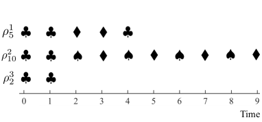
Refer to caption
Figure 1: Three trajectories of different lengths.

Intuitively, if a trajectory of finite length can be extended to infinite length, then the strong view indicates that the truth value of the formula on the infinite-length trajectory is already “determined” on the trajectory of finite length, while the weak view indicates that it may not be “determined” yet. As shown in the simple example in Fig. 1, with the set S={,,}𝑆S=\{\clubsuit,\spadesuit,\blacklozenge\} of states and three trajectories ρ51subscriptsuperscript𝜌15\rho^{1}_{5}, ρ102subscriptsuperscript𝜌210\rho^{2}_{10} and ρ23subscriptsuperscript𝜌32\rho^{3}_{2}, F4subscript𝐹absent4F_{\leq 4}\clubsuit is strongly satisfied by all three trajectories, while F4subscript𝐹absent4F_{\leq 4}\spadesuit is strongly violated by ρ51subscriptsuperscript𝜌15\rho^{1}_{5}, strongly satisfied by ρ102subscriptsuperscript𝜌210\rho^{2}_{10}, and weakly satisfied (and also weakly violated) by ρ23subscriptsuperscript𝜌32\rho^{3}_{2}.

3 Teaching pLTLf Formulas with Demonstrations of Varying Lengths

We now provide the framework for teaching pLTLf formulas with demonstrations (trajectories) of varying lengths.

3.1 Teaching Model

Let 𝒵:=S+×{1,1}assign𝒵superscript𝑆11\mathcal{Z}:=S^{+}\times\{-1,1\} be the ground set of (labeled) demonstrations (trajectories), where S+superscript𝑆S^{+} denotes the Kleene plus of S𝑆S, and {1,1}11\{-1,1\} is the set of labels. There is a hypothesis set Φ={ϕ1,,ϕn}Φsubscriptitalic-ϕ1subscriptitalic-ϕ𝑛\Phi=\{\phi_{1},\dots,\phi_{n}\} consisting of n>0𝑛subscriptabsent0n\in\mathbb{Z}_{>0} hypothesis pLTLf formulas. The teacher knows a target hypothesis ϕΦsuperscriptitalic-ϕΦ\phi^{\ast}\in\Phi and intends to teach ϕsuperscriptitalic-ϕ\phi^{\ast} to a learner.

We define the preference function σ:Φ×Φ>0:𝜎ΦΦsubscriptabsent0\sigma:\Phi\times\Phi\rightarrow\mathbb{R}_{>0} as a function that encodes the learner’s transition preferences. Specifically, given the current hypothesis ϕitalic-ϕ\phi and any two hypotheses ϕsuperscriptitalic-ϕ\phi^{\prime} and ϕ′′superscriptitalic-ϕ′′\phi^{\prime\prime}, ϕsuperscriptitalic-ϕ\phi^{\prime} is preferred to ϕ′′superscriptitalic-ϕ′′\phi^{\prime\prime} from ϕitalic-ϕ\phi if and only if σ(ϕ;ϕ)<σ(ϕ′′;ϕ)𝜎superscriptitalic-ϕitalic-ϕ𝜎superscriptitalic-ϕ′′italic-ϕ\sigma(\phi^{\prime};\phi)<\sigma(\phi^{\prime\prime};\phi). If for any ϕsuperscriptitalic-ϕ\phi^{\prime}, σ(ϕ;ϕ)𝜎superscriptitalic-ϕitalic-ϕ\sigma(\phi^{\prime};\phi) does not depend on ϕitalic-ϕ\phi, then σ𝜎\sigma is a global preference function; otherwise, σ𝜎\sigma is a local preference function. If σ(ϕ;ϕ)𝜎superscriptitalic-ϕitalic-ϕ\sigma(\phi^{\prime};\phi) is a constant for any ϕitalic-ϕ\phi and ϕsuperscriptitalic-ϕ\phi^{\prime}, then σ𝜎\sigma is a uniform preference function.

Definition 3.

Given a target hypothesis ϕsuperscriptitalic-ϕ\phi^{\ast} and a demonstration (ρL,l)subscript𝜌𝐿𝑙(\rho_{L},l), where l=1𝑙1l=1 represents positive demonstration and l=1𝑙1l=-1 represents negative demonstration, (ρL,l)subscript𝜌𝐿𝑙(\rho_{L},l) is strongly inconsistent with a pLTLf formula ϕΦitalic-ϕΦ\phi\in\Phi, if and only if the following condition is satisfied:

{(ρL,0)Sϕ,(ρL,0)S¬ϕ,if l=1;(ρL,0)S¬ϕ,(ρL,0)Sϕ,if l=1.casesformulae-sequencesubscriptmodelsSsubscript𝜌𝐿0superscriptitalic-ϕsubscriptmodelsSsubscript𝜌𝐿0italic-ϕif l=1otherwiseformulae-sequencesubscriptmodelsSsubscript𝜌𝐿0superscriptitalic-ϕsubscriptmodelsSsubscript𝜌𝐿0italic-ϕif l=1otherwise\begin{split}\begin{cases}(\rho_{L},0)\models_{\rm{S}}\phi^{\ast},~{}~{}(\rho_{L},0)\models_{\rm{S}}\lnot\phi,~{}~{}~{}~{}~{}~{}~{}~{}\mbox{if $l=1$};\\ (\rho_{L},0)\models_{\rm{S}}\lnot\phi^{\ast},~{}~{}(\rho_{L},0)\models_{\rm{S}}\phi,~{}~{}~{}~{}~{}~{}~{}~{}\mbox{if $l=-1$}.\end{cases}\\ \end{split}

Starting from the teacher’s first demonstration, the teaching stops as soon as the learner’s current hypothesis reaches the target hypothesis, and we call it a teaching session. For a sequence D𝐷D of demonstrations, we define the version space induced by D𝐷D, denoted as Φ(D)Φ𝐷\Phi(D), as the subset of pLTLf formulas in ΦΦ\Phi that are not strongly inconsistent with any demonstration in D𝐷D. We use ΘΘ\Theta to denote the random variable representing the randomness of the environment (e.g., learner’s random choice of next hypothesis in the presence of ties) and θ𝜃\theta to denote the realization of ΘΘ\Theta in each teaching session.

Definition 4.

We define a teaching setting as a 4-tuple 𝒮=(ϕ,ϕ0,Φ,dom(Θ))𝒮superscriptitalic-ϕsuperscriptitalic-ϕ0ΦdomΘ\mathcal{S}=(\phi^{\ast},\phi^{0},\Phi,\operatorname*{dom}(\Theta)), where ϕsuperscriptitalic-ϕ\phi^{\ast} is the target hypothesis, ϕ0ϕsuperscriptitalic-ϕ0superscriptitalic-ϕ\phi^{0}\neq\phi^{\ast} is the learner’s initial hypothesis, ΦΦ\Phi is the hypothesis set and dom(Θ)domΘ\operatorname*{dom}(\Theta) is the domain of the random variable ΘΘ\Theta.

Let 𝒯𝒯\mathcal{T} be a teacher that outputs a sequence of demonstrations based on the target hypothesis, the version space, and either the learner’s initial hypothesis (non-adaptive teacher) or the learner’s current hypothesis (adaptive teacher). For a learner with preference function σ𝜎\sigma, let σ:Φ×2Φ×𝒵×dom(Θ)Φ:subscript𝜎Φsuperscript2Φ𝒵domΘΦ\mathcal{L}_{\sigma}:\Phi\times 2^{\Phi}\times\mathcal{Z}\times\operatorname*{dom}(\Theta)\rightarrow\Phi be the learner’s mapping that maps the learner’s current hypothesis, the current version space, the current demonstration and the randomness of the environment to the learner’s next updated hypothesis. Given a teacher 𝒯𝒯\mathcal{T}, a learner σsubscript𝜎\mathcal{L}_{\sigma} and the randomness θ𝜃\theta in the teaching setting 𝒮=(ϕ,ϕ0,Φ,dom(Θ))𝒮superscriptitalic-ϕsuperscriptitalic-ϕ0ΦdomΘ\mathcal{S}=(\phi^{\ast},\phi^{0},\Phi,\operatorname*{dom}(\Theta)), we use D𝒮(𝒯,σ,θ)subscript𝐷𝒮𝒯subscript𝜎𝜃D_{\mathcal{S}}(\mathcal{T},\mathcal{L}_{\sigma},\theta) to denote the sequence of demonstrations provided by the teacher 𝒯𝒯\mathcal{T} before the learner’s hypothesis reaches ϕsuperscriptitalic-ϕ\phi^{*}.

Definition 5.

The accumulated-number (AN) teaching cost and accumulated-length (AL) teaching cost are defined as

AN-Cost𝒮(𝒯,σ,θ):=|D𝒮(𝒯,σ,θ)|,AL-Cost𝒮(𝒯,σ,θ):=(ρLkk,lk)D𝒮(𝒯,σ,θ)Lk.formulae-sequenceassignsubscriptAN-Cost𝒮𝒯subscript𝜎𝜃subscript𝐷𝒮𝒯subscript𝜎𝜃assignsubscriptAL-Cost𝒮𝒯subscript𝜎𝜃subscriptsubscriptsuperscript𝜌𝑘subscript𝐿𝑘subscript𝑙𝑘subscript𝐷𝒮𝒯subscript𝜎𝜃subscript𝐿𝑘\begin{split}\textrm{AN-Cost}_{\mathcal{S}}(\mathcal{T},\mathcal{L}_{\sigma},\theta):=&|D_{\mathcal{S}}(\mathcal{T},\mathcal{L}_{\sigma},\theta)|,\\ \textrm{AL-Cost}_{\mathcal{S}}(\mathcal{T},\mathcal{L}_{\sigma},\theta):=&\sum\limits_{(\rho^{k}_{L_{k}},l_{k})\in D_{\mathcal{S}}(\mathcal{T},\mathcal{L}_{\sigma},\theta)}L_{k}.\end{split}

Intuitively, the AN teaching cost and the AL teaching cost are the number of demonstrations and the accumulated time lengths of the demonstrations for the learner’s hypothesis to reach ϕsuperscriptitalic-ϕ\phi^{\ast} in a specific teaching session, respectively.

Definition 6.

Given a teacher 𝒯𝒯\mathcal{T} and a learner σsubscript𝜎\mathcal{L}_{\sigma} in the teaching setting 𝒮=(ϕ,ϕ0,Φ,dom(Θ))𝒮superscriptitalic-ϕsuperscriptitalic-ϕ0ΦdomΘ\mathcal{S}=(\phi^{\ast},\phi^{0},\Phi,\operatorname*{dom}(\Theta)), we define the worst-case AN teaching cost and AL teaching cost as

AN-Cost𝒮WC(𝒯,σ):=maxθdom(Θ)AN-Cost𝒮(𝒯,σ,θ),AL-Cost𝒮WC(𝒯,σ):=maxθdom(Θ)AL-Cost𝒮(𝒯,σ.θ).\begin{split}\textrm{AN-Cost}^{\textrm{WC}}_{\mathcal{S}}(\mathcal{T},\mathcal{L}_{\sigma}):=&\max\limits_{\theta\in\operatorname*{dom}(\Theta)}\textrm{AN-Cost}_{\mathcal{S}}(\mathcal{T},\mathcal{L}_{\sigma},\theta),\\ \textrm{AL-Cost}^{\textrm{WC}}_{\mathcal{S}}(\mathcal{T},\mathcal{L}_{\sigma}):=&\max\limits_{\theta\in\operatorname*{dom}(\Theta)}\textrm{AL-Cost}_{\mathcal{S}}(\mathcal{T},\mathcal{L}_{\sigma}.\theta).\end{split}
Definition 7.

Given a learner σsubscript𝜎\mathcal{L}_{\sigma} in the teaching setting 𝒮=(ϕ,ϕ0,Φ,dom(Θ))𝒮superscriptitalic-ϕsuperscriptitalic-ϕ0ΦdomΘ\mathcal{S}=(\phi^{\ast},\phi^{0},\Phi,\operatorname*{dom}(\Theta)), we define the AN teaching complexity and AL teaching complexity respectively as

AN-Complexity𝒮(σ):=min𝒯AN-Cost𝒮WC(𝒯,σ),AL-Complexity𝒮(σ):=min𝒯AL-Cost𝒮WC(𝒯,σ).formulae-sequenceassignsubscriptAN-Complexity𝒮subscript𝜎subscript𝒯subscriptsuperscriptAN-CostWC𝒮𝒯subscript𝜎assignsubscriptAL-Complexity𝒮subscript𝜎subscript𝒯subscriptsuperscriptAL-CostWC𝒮𝒯subscript𝜎\begin{split}\textrm{AN-Complexity}_{\mathcal{S}}(\mathcal{L}_{\sigma}):=&\min\limits_{\mathcal{T}}\textrm{AN-Cost}^{\textrm{WC}}_{\mathcal{S}}(\mathcal{T},\mathcal{L}_{\sigma}),\\ \textrm{AL-Complexity}_{\mathcal{S}}(\mathcal{L}_{\sigma}):=&\min\limits_{\mathcal{T}}\textrm{AL-Cost}^{\textrm{WC}}_{\mathcal{S}}(\mathcal{T},\mathcal{L}_{\sigma}).\end{split}

Intuitively, the AN teaching complexity and the AL teaching complexity are the minimal number of demonstrations and the minimal accumulated time lengths of the demonstrations needed for the learner’s hypothesis to reach ϕsuperscriptitalic-ϕ\phi^{\ast} despite the randomness of the environment, respectively.

For example, we consider the hypothesis set Φ={Fis}Φsubscript𝐹absent𝑖𝑠\Phi=\{F_{\leq i}s\}, where i{0,,4}𝑖04i\in\{0,\dots,4\}, and sS={,,}𝑠𝑆s\in S=\{\clubsuit,\spadesuit,\blacklozenge\}. If ϕsuperscriptitalic-ϕ\phi^{\ast} is F2subscript𝐹absent2F_{\leq 2}\clubsuit, and the learner has uniform preference, then for any ϕ0superscriptitalic-ϕ0\phi^{0}, one sequence of demonstrations which can minimize both the (worst-case) AN and AL teaching costs222Note that there does not always exist a sequence of demonstrations that minimizes both the AN and AL teaching costs. are firstly a negative demonstration of ,,,,\spadesuit,\blacklozenge,\spadesuit,\clubsuit,\clubsuit, and then a positive demonstration of ,,\spadesuit,\blacklozenge,\clubsuit. In this teaching setting, the AN and AL teaching complexities are 2 and 8, respectively.

3.2 TLIP: Teaching pLTLf Formulas with Integer Programming

Finding the optimal sequence of demonstrations with minimal AN or AL teaching cost has time complexity in the order of 2|DLmax|superscript2subscript𝐷subscript𝐿max2^{|D_{L_{\textrm{max}}}|}, where DLmaxsubscript𝐷subscript𝐿maxD_{L_{\textrm{max}}} is the set of all possible demonstrations with length at most Lmaxsubscript𝐿maxL_{\textrm{max}}. As |DLmax|=i=1Lmax|S|Lmaxsubscript𝐷subscript𝐿maxsuperscriptsubscript𝑖1subscript𝐿maxsuperscript𝑆subscript𝐿max|D_{L_{\textrm{max}}}|=\sum_{i=1}^{L_{\textrm{max}}}|S|^{L_{\textrm{max}}}, 2|DLmax|superscript2subscript𝐷subscript𝐿max2^{|D_{L_{\textrm{max}}}|} is doubly exponential with the maximal length of the demonstrations.

We resort to greedy methods for myopic teaching with near-optimal performance. To compute the greedy solution, we first derive a necessary condition through Definition 8 and Theorem 1 for the minimal time length of a demonstration so that a set of pLTLf formulas are strongly inconsistent with (thus can be eliminated by) this demonstration.

Definition 8.

We define the minimal time length ζ(ϕ,l)𝜁italic-ϕ𝑙\zeta(\phi,l) of a pLTLf formula ϕitalic-ϕ\phi with respect to a label l𝑙l recursively as

ζ(π,l)=0,ζ(¬ϕ,l)=ζ(ϕ,l),ζ(ϕ1ϕ2,l)={max{ζ(ϕ1,l),ζ(ϕ2,l)},if l=1;min{ζ(ϕ1,l),ζ(ϕ2,l)},if l=1,ζ(Fτϕ,l)={ζ(ϕ,l),if l=1;ζ(ϕ,l)+τ,if l=1,ζ(Gτϕ,l)={ζ(ϕ,l)+τ,if l=1;ζ(ϕ,l),if l=1.\begin{split}\zeta(\pi,l)=&0,~{}~{}~{}~{}~{}~{}\zeta(\lnot\phi,l)=\zeta(\phi,-l),\\ \zeta(\phi_{1}\wedge\phi_{2},l)=&\begin{cases}\max\{\zeta(\phi_{1},l),\zeta(\phi_{2},l)\},&\mbox{if $l=1$};\\ \min\{\zeta(\phi_{1},l),\zeta(\phi_{2},l)\},&\mbox{if $l=-1$},\end{cases}\\ \zeta(F_{\leq\tau}\phi,l)=&\begin{cases}\zeta(\phi,l),~{}~{}~{}~{}~{}~{}~{}~{}~{}~{}~{}~{}~{}~{}~{}~{}~{}~{}~{}~{}~{}~{}\mbox{if $l=1$};\\ \zeta(\phi,l)+\tau,~{}~{}~{}~{}~{}~{}~{}~{}~{}~{}~{}~{}~{}~{}~{}\mbox{if $l=-1$},\end{cases}\\ \zeta(G_{\leq\tau}\phi,l)=&\begin{cases}\zeta(\phi,l)+\tau,~{}~{}~{}~{}~{}~{}~{}~{}~{}~{}~{}~{}~{}~{}~{}~{}\mbox{if $l=1$};\\ \zeta(\phi,l),~{}~{}~{}~{}~{}~{}~{}~{}~{}~{}~{}~{}~{}~{}~{}~{}~{}~{}~{}~{}~{}~{}~{}\mbox{if $l=-1$}.\end{cases}\end{split}
Theorem 1.

Given a target hypothesis ϕsuperscriptitalic-ϕ\phi^{\ast} and the hypothesis set ΦΦ\Phi, if a demonstration (ρL,l)subscript𝜌𝐿𝑙(\rho_{L},l) is strongly inconsistent with a subset Φ^={ϕi}i=1N^Φ^Φsubscriptsuperscriptsubscriptitalic-ϕ𝑖^𝑁𝑖1Φ\hat{\Phi}=\{\phi_{i}\}^{\hat{N}}_{i=1}\subset\Phi of pLTLf formulas, then

Lmax{ζ(ϕ,l),max1iN^ζ(ϕi,l)}.𝐿𝜁superscriptitalic-ϕ𝑙subscript1𝑖^𝑁𝜁subscriptitalic-ϕ𝑖𝑙L\geq\max\{\zeta(\phi^{\ast},l),\max\limits_{1\leq i\leq\hat{N}}\zeta(\phi_{i},-l)\}.
1 Input: hypothesis set ΦΦ\Phi, initial hypothesis ϕ0superscriptitalic-ϕ0\phi^{0}
2 Initialize k0𝑘0k\leftarrow 0, Φ~~Φ\tilde{\Phi}\leftarrow\emptyset, Φ0ΦsuperscriptΦ0Φ\Phi^{0}\leftarrow\Phi
3 while ϕkϕsuperscriptitalic-ϕ𝑘superscriptitalic-ϕ\phi^{k}\neq\phi^{\ast} do
4       if MyopicTeacher=1MyopicTeacher1\text{MyopicTeacher}=1 then  ϕk=ϕsuperscriptitalic-ϕ𝑘superscriptitalic-ϕ\phi^{k\ast}=\phi^{\ast}
5       else  Compute ϕkOracle(ϕk,Φk,ϕ)superscriptitalic-ϕ𝑘Oraclesuperscriptitalic-ϕ𝑘superscriptΦ𝑘superscriptitalic-ϕ\phi^{k\ast}\leftarrow\text{Oracle}(\phi^{k},\Phi^{k},\phi^{\ast})
6       if σ𝜎\sigma is global then
7             Φ~{ϕΦk:σ(ϕ;)σ(ϕk;)}~Φconditional-setitalic-ϕsuperscriptΦ𝑘𝜎italic-ϕ𝜎superscriptitalic-ϕ𝑘\tilde{\Phi}\leftarrow\{\phi\in\Phi^{k}:\sigma(\phi;\cdot)\leq\sigma(\phi^{k\ast};\cdot)\}
8      else
9             Φ~{ϕΦk:σ(ϕ;ϕ)σ(ϕk;ϕ)\tilde{\Phi}\leftarrow\{\phi\in\Phi^{k}:\sigma(\phi;\phi^{\prime})\leq\sigma(\phi^{k\ast};\phi^{\prime}) for some ϕΦk}\phi^{\prime}\in\Phi^{k}\}
10       (ρk,k),Φ^superscript𝜌𝑘superscript𝑘^Φabsent(\rho^{k},\ell^{k}),\hat{\Phi}\leftarrowComputeDemonstration(ΦksuperscriptΦ𝑘\Phi^{k}, Φ~~Φ\tilde{\Phi}, ϕksuperscriptitalic-ϕ𝑘\phi^{k\ast})
11       Φk+1ΦkΦ^superscriptΦ𝑘1superscriptΦ𝑘^Φ\Phi^{k+1}\leftarrow\Phi^{k}\setminus\hat{\Phi}, Φ~Φ~Φ^~Φ~Φ^Φ\tilde{\Phi}\leftarrow\tilde{\Phi}\setminus\hat{\Phi}, kk+1𝑘𝑘1k\leftarrow k+1
12       if AdaptiveTeacher=0AdaptiveTeacher0\text{AdaptiveTeacher}=0 then
13             if Φ~={ϕ}~Φsuperscriptitalic-ϕ\tilde{\Phi}=\{\phi^{\ast}\} then ϕkϕsuperscriptitalic-ϕ𝑘superscriptitalic-ϕ\phi^{k}\leftarrow\phi^{\ast}
14             else  Randomly select ϕkϕsuperscriptitalic-ϕ𝑘superscriptitalic-ϕ\phi^{k}\neq\phi^{\ast} from Φ~~Φ\tilde{\Phi}
15            
16      else  Observe the learner’s next hypothesis ϕksuperscriptitalic-ϕ𝑘\phi^{k}
17      
18Kk1𝐾𝑘1K\leftarrow k-1
return {(ρ0,0),(ρ1,1),,(ρK,K)}superscript𝜌0superscript0superscript𝜌1superscript1superscript𝜌𝐾superscript𝐾\{(\rho^{0},\ell^{0}),(\rho^{1},\ell^{1}),\dots,(\rho^{K},\ell^{K})\}
Algorithm 1 Teaching of pLTLf Formulas with Integer Programming (TLIP)
1 Input:Φ,Φ~:InputΦ~Φ\textbf{Input}:\Phi,\tilde{\Phi}, ϕsuperscriptitalic-ϕ\phi^{\ast}
2 Compute ρpossubscriptsuperscript𝜌pos\rho^{\ast}_{\textrm{pos}} and κ(ρpos)𝜅subscriptsuperscript𝜌pos\kappa(\rho^{\ast}_{\textrm{pos}}) for IPpos(Φ~,ϕ)subscriptIPpos~Φsuperscriptitalic-ϕ\textrm{IP}_{\textrm{pos}}(\tilde{\Phi},\phi^{\ast})
3 Compute ρnegsubscriptsuperscript𝜌neg\rho^{\ast}_{\textrm{neg}} and κ(ρneg)𝜅subscriptsuperscript𝜌neg\kappa(\rho^{\ast}_{\textrm{neg}}) for IPneg(Φ~,ϕ)subscriptIPneg~Φsuperscriptitalic-ϕ\textrm{IP}_{\textrm{neg}}(\tilde{\Phi},\phi^{\ast})
4 if κ(ρpos)κ(ρneg)𝜅subscriptsuperscript𝜌pos𝜅subscriptsuperscript𝜌neg\kappa(\rho^{\ast}_{\textrm{pos}})\geq\kappa(\rho^{\ast}_{\textrm{neg}}) then
5       (ρ,)(ρpos,1)𝜌subscriptsuperscript𝜌pos1(\rho,\ell)\leftarrow(\rho^{\ast}_{\textrm{pos}},1), Φ^{ϕΦ:c(ϕ,ρ)=1}^Φconditional-setitalic-ϕΦ𝑐italic-ϕ𝜌1\hat{\Phi}\leftarrow\{\phi\in\Phi:c(\phi,\rho)=-1\}
6else
7       (ρ,)(ρneg,1)𝜌subscriptsuperscript𝜌neg1(\rho,\ell)\leftarrow(\rho^{\ast}_{\textrm{neg}},-1), Φ^{ϕΦ:c(ϕ,ρ)=1}^Φconditional-setitalic-ϕΦ𝑐italic-ϕ𝜌1\hat{\Phi}\leftarrow\{\phi\in\Phi:c(\phi,\rho)=1\}
return (ρ,)𝜌(\rho,\ell), Φ^^Φ\hat{\Phi}
Algorithm 2 ComputeDemonstration

Algorithm 1 shows the proposed TLIP approach for teaching pLTLf formulas to learners with preferences. Here we focus on the myopic solution (MyopicTeacher=1MyopicTeacher1\textit{MyopicTeacher}=1) under the non-adaptive setting (AdaptiveTeacher=0AdaptiveTeacher0\textit{AdaptiveTeacher}=0) where the teacher does not observe the learner’s current hypothesis and provides the sequence of demonstrations based on the learner’s initial hypothesis. We compute Φ~~Φ\tilde{\Phi} as either (i) the set of hypotheses that are preferred over the target hypothesis in the current version space if the learner has global preferences (Line 1), or (ii) the union of the sets of hypotheses that are preferred over target hypothesis based on each hypothesis in the current version space if the learner has local preferences (Line 1). Then we call Algorithm 2 to compute the demonstrations that achieve the greedy myopic solution (Line 1).

Note that finding the greedy myopic solution via exhaustive search amounts to traversing the space of demonstrations, which is exponential with the maximal length of the demonstrations. We propose to find the greedy solution via a novel integer programming (IP) formulation. For a trajectory ρLsubscript𝜌𝐿\rho_{L} and a pLTLf formula ϕitalic-ϕ\phi, we denote c(ϕ,ρL)=1𝑐italic-ϕsubscript𝜌𝐿1c(\phi,\rho_{L})=1 if (ρL,0)SϕsubscriptmodelsSsubscript𝜌𝐿0italic-ϕ(\rho_{L},0)\models_{\rm{S}}\phi; c(ϕ,ρL)=1𝑐italic-ϕsubscript𝜌𝐿1c(\phi,\rho_{L})=-1 if (ρL,0)S¬ϕsubscriptmodelsSsubscript𝜌𝐿0italic-ϕ(\rho_{L},0)\models_{\rm{S}}\lnot\phi; and c(ϕ,ρL)=0𝑐italic-ϕsubscript𝜌𝐿0c(\phi,\rho_{L})=0 if (ρL,0)⊧̸Sϕsubscriptnot-modelsSsubscript𝜌𝐿0italic-ϕ(\rho_{L},0)\not\models_{\rm{S}}\phi and (ρL,0)⊧̸S¬ϕsubscriptnot-modelsSsubscript𝜌𝐿0italic-ϕ(\rho_{L},0)\not\models_{\rm{S}}\lnot\phi. For positive demonstrations, we compute the following integer programming problem IPpos(Φ~,ϕ)subscriptIPpos~Φsuperscriptitalic-ϕ\textrm{IP}_{\textrm{pos}}(\tilde{\Phi},\phi^{\ast}).

maxρLκ(ρL)subject to:bj{0,1},j,s.t.ϕjΦ~,c(ϕ,ρL)=1,c(ϕj,ρL)=12bj,j,s.t.ϕjΦ~,Lζ(ϕ,1),Lbjζ(ϕj,1),j,s.t.ϕjΦ~,formulae-sequencesubscriptsubscript𝜌𝐿𝜅subscript𝜌𝐿subject to:subscript𝑏𝑗01for-all𝑗formulae-sequences.t.subscriptitalic-ϕ𝑗~Φformulae-sequence𝑐superscriptitalic-ϕsubscript𝜌𝐿1formulae-sequence𝑐subscriptitalic-ϕ𝑗subscript𝜌𝐿12subscript𝑏𝑗for-all𝑗formulae-sequences.t.subscriptitalic-ϕ𝑗~Φformulae-sequence𝐿𝜁superscriptitalic-ϕ1formulae-sequence𝐿subscript𝑏𝑗𝜁subscriptitalic-ϕ𝑗1for-all𝑗s.t.subscriptitalic-ϕ𝑗~Φ\begin{split}\max_{\rho_{L}}~{}&\kappa(\rho_{L})\\ \text{subject to:}~{}&b_{j}\in\{0,1\},\forall j,~{}\mbox{s.t.}~{}\phi_{j}\in\tilde{\Phi},~{}~{}c(\phi^{\ast},\rho_{L})=1,\\ &c(\phi_{j},\rho_{L})=1-2b_{j},\forall j,~{}\mbox{s.t.}~{}\phi_{j}\in\tilde{\Phi},\\ &L\geq\zeta(\phi^{\ast},1),L\geq b_{j}\zeta(\phi_{j},-1),\forall j,~{}\mbox{s.t.}~{}\phi_{j}\in\tilde{\Phi},\end{split}

where κ(ρL)=(ϕjΦ~bj)𝜅subscript𝜌𝐿subscriptsubscriptitalic-ϕ𝑗~Φsubscript𝑏𝑗\kappa(\rho_{L})=\big{(}\sum_{\phi_{j}\in\tilde{\Phi}}b_{j}\big{)} when optimizing for the AN teaching cost and κ(ρL)=(ϕjΦ~bj)/L𝜅subscript𝜌𝐿subscriptsubscriptitalic-ϕ𝑗~Φsubscript𝑏𝑗𝐿\kappa(\rho_{L})=\big{(}\sum_{\phi_{j}\in\tilde{\Phi}}b_{j}\big{)}/L when optimizing for the AL teaching cost, the strong satisfaction or strong violation of a pLTLf formula ϕitalic-ϕ\phi by ρLsubscript𝜌𝐿\rho_{L} can be encoded as integer linear constraints of ρLsubscript𝜌𝐿\rho_{L}, and the constraints for L𝐿L are obtained from Theorem 1. In practice, the problem IPpos(Φ~,ϕ)subscriptIPpos~Φsuperscriptitalic-ϕ\textrm{IP}_{\textrm{pos}}(\tilde{\Phi},\phi^{\ast}) can be efficiently solved by highly-optimized IP solvers [32], which, as demonstrated in §5, is significantly more efficient than the exhaustive search method.

For negative demonstrations, the integer programming problem IPneg(Φ~,ϕ)subscriptIPneg~Φsuperscriptitalic-ϕ\textrm{IP}_{\textrm{neg}}(\tilde{\Phi},\phi^{\ast}) can be similarly formulated with the constraints c(ϕ,ρL)=1𝑐superscriptitalic-ϕsubscript𝜌𝐿1c(\phi^{\ast},\rho_{L})=-1 and c(ϕj,ρL)=1+2bj,j,s.t.ϕjΦ~formulae-sequence𝑐subscriptitalic-ϕ𝑗subscript𝜌𝐿12subscript𝑏𝑗for-all𝑗s.t.subscriptitalic-ϕ𝑗~Φc(\phi_{j},\rho_{L})=-1+2b_{j},\forall j,~{}\mbox{s.t.}~{}\phi_{j}\in\tilde{\Phi}. We use ρpossubscriptsuperscript𝜌pos\rho^{\ast}_{\textrm{pos}} and ρnegsubscriptsuperscript𝜌neg\rho^{\ast}_{\textrm{neg}} to denote the optimal positive and negative demonstration computed from IPpos(Φ~,ϕ)subscriptIPpos~Φsuperscriptitalic-ϕ\textrm{IP}_{\textrm{pos}}(\tilde{\Phi},\phi^{\ast}) and IPneg(Φ~,ϕ)subscriptIPneg~Φsuperscriptitalic-ϕ\textrm{IP}_{\textrm{neg}}(\tilde{\Phi},\phi^{\ast}), respectively. We select ρpossubscriptsuperscript𝜌pos\rho^{\ast}_{\textrm{pos}} or ρnegsubscriptsuperscript𝜌neg\rho^{\ast}_{\textrm{neg}} depending on whether κ(ρpos)𝜅subscriptsuperscript𝜌pos\kappa(\rho^{\ast}_{\textrm{pos}}) is no less than κ(ρneg)𝜅subscriptsuperscript𝜌neg\kappa(\rho^{\ast}_{\textrm{neg}}) or not. Then, we eliminate the hypothesis pLTLf formulas that are strongly inconsistent with the selected demonstration (Line 1). For non-adaptive teaching, we randomly select a pLTLf formula different from the target hypothesis (Line 1, as we consider the worst case) and perform another round of computation for the demonstration until the current hypothesis reaches the target hypothesis.

3.3 Teaching with Positive Demonstrations Only

Learning temporal logic formulas from positive demonstrations is a typical problem in temporal logic inference [22, 3, 28].

The algorithm for teaching pLTLf formulas with positive demonstrations only can be modified from Algorithms 1 and 2, by deleting Lines 3-7 of Algorithm 2 and obtaining (ρ,l)𝜌𝑙(\rho,l) as (ρpos,1)subscriptsuperscript𝜌pos1(\rho^{\ast}_{\textrm{pos}},1). The following theorem provides a necessary condition for successfully teaching a pLTLf formula with positive demonstrations to a learner with global preferences.

Theorem 2.

Given a hypothesis set ΦΦ\Phi and a sequence of positive demonstrations Dpsubscript𝐷pD_{\textrm{p}}, if a target hypothesis ϕΦsuperscriptitalic-ϕΦ\phi^{\ast}\in\Phi is teachable from Dpsubscript𝐷pD_{\textrm{p}} to a learner with global preference function σ𝜎\sigma, i.e., ϕΦ(D){ϕ},σ(ϕ;)>σ(ϕ;)formulae-sequencefor-allitalic-ϕΦ𝐷superscriptitalic-ϕ𝜎italic-ϕ𝜎superscriptitalic-ϕ\forall\phi\in\Phi(D)\setminus\{\phi^{\ast}\},\sigma(\phi;\cdot)>\sigma(\phi^{\ast};\cdot), then it holds that max1k|Dp|LkmaxϕiΦ~{ϕ}ζ(ϕi,1)subscript1𝑘subscript𝐷psubscript𝐿𝑘subscriptsubscriptitalic-ϕ𝑖~Φsuperscriptitalic-ϕ𝜁subscriptitalic-ϕ𝑖1\max\limits_{1\leq k\leq|D_{\textrm{p}}|}L_{k}\geq\max\limits_{\phi_{i}\in\tilde{\Phi}\setminus\{\phi^{\ast}\}}\zeta(\phi_{i},-1), and that there does not exist a pLTLf formula ϕsuperscriptitalic-ϕ\phi^{\prime} with σ(ϕ;)σ(ϕ;)𝜎superscriptitalic-ϕ𝜎superscriptitalic-ϕ\sigma(\phi^{\prime};\cdot)\leq\sigma(\phi^{\ast};\cdot) such that ϕϕsuperscriptitalic-ϕsuperscriptitalic-ϕ\phi^{\ast}\Rightarrow\phi^{\prime}. Here, Φ~:={ϕΦ:σ(ϕ;)σ(ϕ;)}assign~Φconditional-setitalic-ϕΦ𝜎italic-ϕ𝜎superscriptitalic-ϕ\tilde{\Phi}:=\{\phi\in\Phi:\sigma(\phi;\cdot)\leq\sigma(\phi^{\ast};\cdot)\}, Lksubscript𝐿𝑘L_{k} is the time length of the k𝑘k-th demonstration in Dpsubscript𝐷pD_{\textrm{p}}, and ζ(ϕi,1)𝜁subscriptitalic-ϕ𝑖1\zeta(\phi_{i},-1) is as defined in Definition 8.

4 Adaptive Teaching of pLTLf Formulas

We now explore the theoretical aspects of machine teaching for pLTLf formulas under the adaptive setting.

4.1 Teaching Complexity

Different from non-adaptive teaching, an adaptive teacher observes the learner’s current hypothesis and provides the next demonstration according to the target hypothesis, the current version space and the learner’s current hypothesis. Algorithm 1 with AdaptiveTeacher=1AdaptiveTeacher1\textit{AdaptiveTeacher}=1 shows the procedure for adaptive teaching using TLIP.

The following theorem provides near-optimality guarantees under the adaptive myopic setting [15].

Theorem 3.

We denote the myopic adaptive teacher in TLIP as 𝒯msuperscript𝒯m\mathcal{T}^{\textrm{m}}. Given a target hypothesis ϕsuperscriptitalic-ϕ\phi^{\ast} and the hypothesis set ΦΦ\Phi, then

AN-Cost𝒮WC(𝒯m,σ)λ(log|Φ~𝒮|+1)AN-Complexity𝒮(σ),AL-Cost𝒮WC(𝒯m,σ)λ(log|Φ~𝒮|+1)AL-Complexity𝒮(σ),formulae-sequencesubscriptsuperscriptAN-CostWC𝒮superscript𝒯msubscript𝜎𝜆subscript~Φ𝒮1subscriptAN-Complexity𝒮subscript𝜎subscriptsuperscriptAL-CostWC𝒮superscript𝒯msubscript𝜎𝜆subscript~Φ𝒮1subscriptAL-Complexity𝒮subscript𝜎\begin{split}\textrm{AN-Cost}^{\textrm{WC}}_{\mathcal{S}}(\mathcal{T}^{\textrm{m}},\mathcal{L}_{\sigma})\leq\lambda(\log|\tilde{\Phi}_{\mathcal{S}}|+1)\textrm{AN-Complexity}_{\mathcal{S}}(\mathcal{L}_{\sigma}),\\ \textrm{AL-Cost}^{\textrm{WC}}_{\mathcal{S}}(\mathcal{T}^{\textrm{m}},\mathcal{L}_{\sigma})\leq\lambda(\log|\tilde{\Phi}_{\mathcal{S}}|+1)\textrm{AL-Complexity}_{\mathcal{S}}(\mathcal{L}_{\sigma}),\end{split}

where Φ~𝒮:={ϕΦ:σ(ϕ;ϕ0)σ(ϕ;ϕ0)}assignsubscript~Φ𝒮conditional-setitalic-ϕΦ𝜎italic-ϕsuperscriptitalic-ϕ0𝜎superscriptitalic-ϕsuperscriptitalic-ϕ0\tilde{\Phi}_{\mathcal{S}}:=\{\phi\in\Phi:\sigma(\phi;\phi^{0})\leq\sigma(\phi^{\ast};\phi^{0})\}, λ=1𝜆1\lambda=1 if σ𝜎\sigma is global, and λ=2𝜆2\lambda=2 if σ𝜎\sigma is local and the following two conditions are satisfied for both σ𝜎\sigma and the sequence D𝐷D of demonstrations.

{1.ϕ,ϕ′′Φ,σ(ϕ;ϕ)σ(ϕ′′;ϕ)σ(ϕ;ϕ)σ(ϕ′′;ϕ)σ(ϕ;ϕ);2.ΦΦ¯({(ρ,l)}),(ρ,l)D,s.t.,Φ¯({(ρ,l)})=Φ.\begin{split}\begin{cases}1.\forall\phi^{\prime},\phi^{\prime\prime}\in\Phi,\sigma(\phi^{\prime};\phi)\leq\sigma(\phi^{\prime\prime};\phi)\leq\sigma(\phi^{\ast};\phi)\\ ~{}~{}~{}~{}~{}~{}~{}~{}~{}~{}~{}~{}~{}~{}~{}~{}~{}~{}\Rightarrow\sigma(\phi^{\prime\prime};\phi^{\prime})\leq\sigma(\phi^{\ast};\phi^{\prime});\\ 2.\forall\Phi^{\prime}\subset\bar{\Phi}(\{(\rho,l)\}),\exists(\rho^{\prime},l^{\prime})\in D,s.t.,\bar{\Phi}(\{(\rho^{\prime},l^{\prime})\})=\Phi^{\prime}.\end{cases}\\ \end{split}

In Condition 2, Φ¯({(ρ,l)})¯Φ𝜌𝑙\bar{\Phi}(\{(\rho,l)\}) denotes the set of hypotheses in ΦΦ\Phi which are strongly inconsistent with demonstration (ρ,l)𝜌𝑙(\rho,l).

Theorem 3 shows that, under the adaptive myopic setting, TLIP can achieve near-optimal performance for global preferences and certain local preferences that satisfy Conditions 1 and 2. This motivates us to design intermediate target hypotheses as shown in §4.2.

4.2 Teaching with Oracles

For learners with local preferences, we can design intermediate target hypotheses so that Condition 1 of Theorem 3 can be satisfied for learning each target hypothesis. In Algorithm 1, we assume that we have access to an oracle, i.e., Oracle(ϕk,Φk,ϕ)Oraclesuperscriptitalic-ϕ𝑘superscriptΦ𝑘superscriptitalic-ϕ\text{Oracle}(\phi^{k},\Phi^{k},\phi^{\ast}), which outputs an intermediate target hypothesis ϕksuperscriptitalic-ϕ𝑘\phi^{k\ast} at each step.

For example, if the learner’s current hypothesis ϕcsuperscriptitalic-ϕc\phi^{\textrm{c}} does not contain \clubsuit, then the learner prefers formulas with the same temporal operator as that in ϕcsuperscriptitalic-ϕc\phi^{\textrm{c}}; and if ϕcsuperscriptitalic-ϕc\phi^{\textrm{c}} contains \clubsuit, then the learner prefers G-formulas than F-formulas. With the same temporal operator, the learner prefers formulas with \spadesuit than formulas with \clubsuit, and prefers formulas with \blacklozenge the least. Then, for ϕ=G2superscriptitalic-ϕsubscript𝐺absent2\phi^{\ast}=G_{\leq 2}\clubsuit, ϕ1=F3superscriptitalic-ϕ1subscript𝐹absent3\phi^{1}=F_{\leq 3}\spadesuit, ϕ2=F5superscriptitalic-ϕ2subscript𝐹absent5\phi^{2}=F_{\leq 5}\clubsuit, ϕ3=F3superscriptitalic-ϕ3subscript𝐹absent3\phi^{3}=F_{\leq 3}\blacklozenge, we have σ(ϕ2;ϕ1)<σ(ϕ3;ϕ1)<σ(ϕ;ϕ1)𝜎superscriptitalic-ϕ2superscriptitalic-ϕ1𝜎superscriptitalic-ϕ3superscriptitalic-ϕ1𝜎superscriptitalic-ϕsuperscriptitalic-ϕ1\sigma(\phi^{2};\phi^{1})<\sigma(\phi^{3};\phi^{1})<\sigma(\phi^{\ast};\phi^{1}), but σ(ϕ;ϕ2)<σ(ϕ3;ϕ2)𝜎superscriptitalic-ϕsuperscriptitalic-ϕ2𝜎superscriptitalic-ϕ3superscriptitalic-ϕ2\sigma(\phi^{\ast};\phi^{2})<\sigma(\phi^{3};\phi^{2}). Therefore, Condition 1 of Theorem 3 does not hold. If the oracle outputs ϕ2superscriptitalic-ϕ2\phi^{2} as an intermediate target hypothesis before the learner’s hypothesis reaches ϕ2superscriptitalic-ϕ2\phi^{2}, then the teaching problem is decomposed into two subproblems, i.e., teaching before ϕ2superscriptitalic-ϕ2\phi^{2} and after ϕ2superscriptitalic-ϕ2\phi^{2}, and both subproblems satisfy Condition 1 of Theorem 3.

5 Experiments

In this section, we evaluate the proposed approach under different teaching settings. The hypothesis set of pLTLf formulas are listed in Table 1. The set S𝑆S of states is {0,1,,10}0110\{0,1,\dots,10\}. In each teaching session, we randomly select both the initial hypothesis and the target hypothesis from the hypothesis set. All results are averaged over 10 teaching sessions.

Table 1: Hypothesis set of pLTLf formulas (a=5,10,15𝑎51015a=5,10,15 correspond to hypothesis sets of sizes 90, 180 and 270, respectively).
Category Hypothesis pLTLf Formulas
F-formulas F1(x1)subscript𝐹absent1𝑥1F_{\leq 1}(x\leq 1), …,F1(x9)subscript𝐹absent1𝑥9F_{\leq 1}(x\leq 9),

Fa(x1)subscript𝐹absent𝑎𝑥1F_{\leq a}(x\leq 1), …,Fa(x9)subscript𝐹absent𝑎𝑥9F_{\leq a}(x\leq 9)
G-formulas G1(x1)subscript𝐺absent1𝑥1G_{\leq 1}(x\leq 1), …, G1(x9)subscript𝐺absent1𝑥9G_{\leq 1}(x\leq 9),

Ga(x1)subscript𝐺absent𝑎𝑥1G_{\leq a}(x\leq 1), …, Ga(x9)subscript𝐺absent𝑎𝑥9G_{\leq a}(x\leq 9)

5.1 Teaching pLTLf Formulas under Global Preferences

We first compare TLIP with the exhaustive search method for myopic teaching (ESMT). Table 2 shows the computation time for TLIP using myopic teaching and ESMT (minimizing the AL teaching costs) for learners with uniform preferences, where timeout (TO) is 300 minutes. ESMT becomes intractable when the maximal length Lmaxsubscript𝐿maxL_{\textrm{max}} of the demonstrations reaches 10 or above, while TLIP maintains relatively short computation time with increasing Lmaxsubscript𝐿maxL_{\textrm{max}}.

Table 2: Computation time for computing the myopic solution.
Lmax=5subscript𝐿max5L_{\textrm{max}}=5 Lmax=10subscript𝐿max10L_{\textrm{max}}=10 Lmax=15subscript𝐿max15L_{\textrm{max}}=15
TLIP 3.67 s 5.29 s 7.65 s
ESMT 4.57 s TO TO

As ESMT is not scalable, we implement the following four methods for comparison for myopic teaching performances.

  • AN-TLIP: TLIP for minimizing AN teaching cost.

  • AL-TLIP: TLIP for minimizing AL teaching cost.

  • AN-RG: randomized greedy algorithm for minimizing AN teaching cost. At each iteration, we greedily pick the demonstration with minimal AN teaching cost among a randomly selected subset of demonstrations.

  • AL-RG: same with AN-RG except that here we minimize the AL teaching cost.
Refer to caption
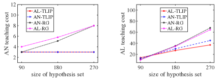
Figure 2: AN and AL teaching costs under global (uniform) preference with increasing sizes of the hypothesis set.

Fig. 2 shows that AN-TLIP (resp. AL-TLIP) outperforms the other three methods when minimizing the AN teaching costs (resp. the AL teaching costs). Specifically, the AN teaching costs using AN-TLIP are 50%, 78.26% and 80.39% less than those using AL-TLIP, AN-RG and AL-RG, respectively. The AL teaching costs using AL-TLIP are 52.63%, 91.37% and 90.23% less than those using AN-TLIP, AN-RG and AL-RG, respectively. Fig. 2 also shows that the growth of the AL teaching cost is more significant with the increasing size of the hypothesis set than that of the AN teaching costs.

Teaching with Positive Demonstrations Only

We test the machine teaching algorithm with positive demonstrations only. We consider global preferences, where the learner prefers F-formulas than G-formulas, and with the same temporal operator the learner prefers formula ϕ1subscriptitalic-ϕ1\phi_{1} than ϕ2subscriptitalic-ϕ2\phi_{2} if and only if ϕ1subscriptitalic-ϕ1\phi_{1} implies ϕ2subscriptitalic-ϕ2\phi_{2}. It can be shown that this preference function satisfies the condition of Theorem 2.
Refer to caption
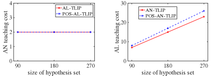
Figure 3: AN and AL teaching costs with positive demonstrations only and with both positive and negative demonstrations with increasing sizes of the hypothesis set.

The corresponding algorithms for AN-TLIP and AL-TLIP with positive demonstrations only are referred to as POS-AN-TLIP and POS-AL-TLIP, respectively. Fig. 3 shows that POS-AN-TLIP and POS-AL-TLIP do not incur much additional teaching cost (up to 20% more) when restricted to only positive demonstrations.

5.2 Teaching pLTLf Formulas under Local Preferences
Refer to caption
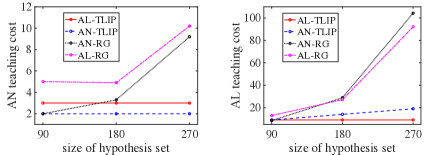
Figure 4: AN and AL teaching costs for adaptive and non-adaptive teaching with increasing sizes of the hypothesis set.

Local preferences

For two pLTLf formulas ϕ1=Fi1(xv1)subscriptitalic-ϕ1subscript𝐹absentsubscript𝑖1𝑥subscript𝑣1\phi_{1}=F_{\leq i_{1}}(x\leq v_{1}) and ϕ2=Fi2(xv2)subscriptitalic-ϕ2subscript𝐹absentsubscript𝑖2𝑥subscript𝑣2\phi_{2}=F_{\leq i_{2}}(x\leq v_{2}), we define the Manhattan distance between ϕ1subscriptitalic-ϕ1\phi_{1} and ϕ2subscriptitalic-ϕ2\phi_{2} as |i1i2|+|v1v2|subscript𝑖1subscript𝑖2subscript𝑣1subscript𝑣2|i_{1}-i_{2}|+|v_{1}-v_{2}|. We consider the following local preference:
(1) The learner prefers formulas with the same temporal operator as that in the learner’s previous hypothesis;
(2) With the same temporal operator the learner prefers formulas that are “closer” to the learner’s previous hypothesis in terms of the Manhattan distance;
(3) The learner prefers G-formulas than F-formulas if the learner’s current hypothesis are in the form of Fi(x0)subscript𝐹absent𝑖𝑥0F_{\leq i}(x\leq 0) or Fi(x10)subscript𝐹absent𝑖𝑥10F_{\leq i}(x\leq 10) (i=1,,a𝑖1𝑎i=1,\dots,a). This is intuitively consistent with human’s preferences to switch categories when the values reach certain boundary values.

Adaptive Teaching

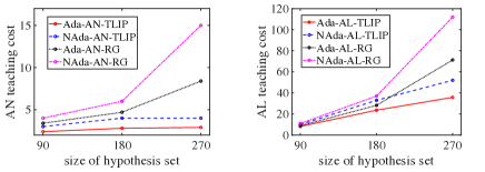
To test the advantage of adaptive teaching, we compare it with non-adaptive teaching in the presence of uncertainties. We consider local preferences with added uncertainty noises. Specifically, the learner has equal preference of selecting the formulas in the version space that have the least Manhattan distance from the current hypothesis and also any formula that can be perturbed from these formulas in the version space (here “perturb” means adding or subtracting the parameters i𝑖i or v𝑣v by 1, e.g., as in Fi(xv)subscript𝐹absent𝑖𝑥𝑣F_{\leq i}(x\leq v)).

Fig. 8 shows that Ada-AN-TLIP (i.e., adaptive AN-TLIP) can reduce the AN teaching costs by up to 27.5% compared with NAda-AN-TLIP (i.e., non-adaptive AN-TLIP), Ada-AN-RG (i.e., adaptive AN-RG) can reduce the AN teaching costs by up to 44% compared with NAda-AN-RG (i.e., non-adaptive AN-RG), Ada-AL-TLIP (i.e., adaptive AL-TLIP) can reduce the AN teaching costs by up to 31.15% compared with NAda-AL-TLIP (i.e., non-adaptive AL-TLIP), and Ada-AL-RG (i.e., adaptive AL-RG) can reduce the AN teaching costs by up to 36.34% compared with NAda-AL-RG (i.e., non-adaptive AL-RG).

Adaptive Teaching with Oracles
Refer to caption
Figure 5: AN and AL teaching costs for adaptive teaching with oracles and without oracles with increasing sizes of the hypothesis set.

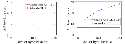
To decompose the teaching problem into subproblems that satisfy Condition 1 of Theorem 3, we design the oracle which outputs an intermediate target hypothesis F1(x10)subscript𝐹absent1𝑥10F_{\leq 1}(x\leq 10)333Theoretically, the oracle can be designed to output any formula of the form Fi(x0)subscript𝐹absent𝑖𝑥0F_{\leq i}(x\leq 0) or Fi(x10)subscript𝐹absent𝑖𝑥10F_{\leq i}(x\leq 10) (i=1,,a𝑖1𝑎i=1,\dots,a).. Fig. 5 shows that Oracle-Ada-AN-TLIP (adaptive AN-TLIP with oracles) can reduce the AN teaching costs by 25% compared with Ada-AN-TLIP and Oracle-Ada-AL-TLIP (adaptive AL-TLIP with oracles) can reduce the AL teaching costs by up to 75% compared with Ada-AL-TLIP.

6 Conclusion

We presented the first attempt for teaching parametric linear temporal logic formulas to a learner with preferences. We also explored how to more efficiently teach the learner utilizing adaptivity and oracles. The results show the effectiveness of the proposed approach. We believe this is an important step towards practical algorithms for teaching more complex concept classes in the real-world scenarios. For future work, we will explore teaching methods for more general forms of temporal logic formulas, with more specific learning algorithms for inferring temporal logic formulas.

References

  • [1] X. Zhu, “Machine teaching: An inverse problem to machine learning and an approach toward optimal education,” ser. AAAI, 2015, pp. 4083–4087. [Online]. Available: http://dl.acm.org/citation.cfm?id=2888116.2888288
  • [2] Z. Kong, A. Jones, and C. Belta, “Temporal logics for learning and detection of anomalous behavior,” IEEE TAC, vol. 62, no. 3, pp. 1210–1222, Mar. 2017.
  • [3] M. Vazquez-Chanlatte, S. Jha, A. Tiwari, M. K. Ho, and S. A. Seshia, “Learning task specifications from demonstrations,” in NeurIPS, 2018, pp. 5372–5382.
  • [4] S. Dasgupta, D. Hsu, S. Poulis, and X. Zhu, “Teaching a black-box learner,” in International Conference on Machine Learning, 2019, pp. 1547–1555.
  • [5] Y. Ma, X. Zhang, W. Sun, and J. Zhu, “Policy poisoning in batch reinforcement learning and control,” in Advances in Neural Information Processing Systems, 2019, pp. 14 543–14 553.
  • [6] S. A. Goldman and M. J. Kearns, “On the complexity of teaching,” Journal of Computer and System Sciences, vol. 50, no. 1, pp. 20–31, 1995.
  • [7] A. Pnueli, “The temporal logic of programs,” in Proc. 18th Annu. Symp. Found. Computer Sci., Washington, D.C., USA, 1977, pp. 46–57.
  • [8] H. Kress-Gazit, T. Wongpiromsarn, and U. Topcu, “Correct, reactive, high-level robot control,” IEEE Robotics Automation Magazine, vol. 18, no. 3, pp. 65–74, Sept 2011.
  • [9] S. T. To, M. Roberts, homas Apker, B. Johnson, and D. W. Aha, “Mixed propositional metric temporal logic: A new formalism for temporal planning.” in AAAI Workshop on Planning for Hybrid Systems.   Phoenix, AZ: AAAI Press, 2015. [Online]. Available: http://www.knexusresearch.com/wp-content/uploads/2016/03/AAAI16.pdf
  • [10] S. Chakraborty and J.-P. Katoen, “Parametric LTL on Markov chains,” in Theoretical Computer Science.   Berlin, Heidelberg: Springer Berlin Heidelberg, 2014, pp. 207–221.
  • [11] R. Alur, K. Etessami, S. La Torre, and D. Peled, “Parametric temporal logic for “Model Measuring”,” ACM Trans. Comput. Logic, vol. 2, no. 3, pp. 388–407, Jul. 2001.
  • [12] O. Mac Aodha, S. Su, Y. Chen, P. Perona, and Y. Yue, “Teaching categories to human learners with visual explanations,” in CVPR, 2018, pp. 3820–3828.
  • [13] D. S. Brown and S. Niekum, “Machine teaching for inverse reinforcement learning: Algorithms and applications,” in Proceedings of the AAAI Conference on Artificial Intelligence, vol. 33, 2019, pp. 7749–7758.
  • [14] Z. Gao, C. Ries, H. U. Simon, and S. Zilles, “Preference-based teaching,” The Journal of Machine Learning Research, vol. 18, no. 1, pp. 1012–1043, 2017.
  • [15] Y. Chen, A. Singla, O. M. Aodha, P. Perona, and Y. Yue, “Understanding the role of adaptivity in machine teaching: The case of version space learners,” in Proc. Conference on Neural Information Processing Systems (NIPS), December 2018.
  • [16] F. Mansouri, Y. Chen, A. Vartanian, J. Zhu, and A. Singla, “Preference-based batch and sequential teaching: Towards a unified view of models,” in Advances in Neural Information Processing Systems, 2019, pp. 9195–9205.
  • [17] J. Zhu, “Machine teaching for bayesian learners in the exponential family,” in Advances in Neural Information Processing Systems, 2013, pp. 1905–1913.
  • [18] W. Liu, B. Dai, A. Humayun, C. Tay, C. Yu, L. B. Smith, J. M. Rehg, and L. Song, “Iterative machine teaching,” in Proceedings of the 34th International Conference on Machine Learning-Volume 70.   JMLR. org, 2017, pp. 2149–2158.
  • [19] B. Hoxha, A. Dokhanchi, and G. Fainekos, “Mining parametric temporal logic properties in model-based design for cyber-physical systems,” International Journal on Software Tools for Technology Transfer, pp. 79–93, Feb 2017. [Online]. Available: http://dx.doi.org/10.1007/s10009-017-0447-4
  • [20] G. Bombara, C.-I. Vasile, F. Penedo, H. Yasuoka, and C. Belta, “A decision tree approach to data classification using signal temporal logic,” in Proc. HSCC’16, 2016, pp. 1–10.
  • [21] D. Neider and I. Gavran, “Learning linear temporal properties,” in Formal Methods in Computer Aided Design (FMCAD), 2018, pp. 1–10.
  • [22] Z. Xu, M. Ornik, A. Julius, and U. Topcu, “Information-guided temporal logic inference with prior knowledge,” in ACC, 2019. [Online]. Available: https://arxiv.org/abs/1811.08846
  • [23] Z. Xu and U. Topcu, “Transfer of temporal logic formulas in reinforcement learning,” in Proc. IJCAI’2019, 7 2019, pp. 4010–4018. [Online]. Available: https://doi.org/10.24963/ijcai.2019/557
  • [24] Z. Xu, M. Birtwistle, C. Belta, and A. Julius, “A temporal logic inference approach for model discrimination,” IEEE Life Sciences Letters, vol. 2, no. 3, pp. 19–22, Sept 2016.
  • [25] Z. Xu, S. Saha, B. Hu, S. Mishra, and A. Julius, “Advisory temporal logic inference and controller design for semi-autonomous robots,” IEEE Trans. Autom. Sci. and Eng., may 2018, in press.
  • [26] Z. Xu and A. Julius, “Census signal temporal logic inference for multiagent group behavior analysis,” IEEE Trans. Autom. Sci. Eng., vol. 15, no. 1, pp. 264–277, Jan. 2018.
  • [27] A. J. Zhe Xu, Calin Belta, “Temporal logic inference with prior information: An application to robot arm movements,” in 5th IFAC Conference on Analysis and Design of Hybrid Systems (ADHS), 2015.
  • [28] A. Shah, P. Kamath, J. A. Shah, and S. Li, “Bayesian inference of temporal task specifications from demonstrations,” in NeurIPS.   Curran Associates, Inc., 2018, pp. 3808–3817. [Online]. Available: http://papers.nips.cc/paper/7637-bayesian-inference-of-temporal-task-specifications-from-demonstrations.pdf
  • [29] C. Eisner, D. Fisman, J. Havlicek, Y. Lustig, A. McIsaac, and D. Van Campenhout, Reasoning with Temporal Logic on Truncated Paths.   Berlin, Heidelberg: Springer Berlin Heidelberg, 2003, pp. 27–39.
  • [30] O. Kupferman and M. Y. Vardi, “Model checking of safety properties,” Form. Methods Syst. Des., vol. 19, no. 3, pp. 291–314, Oct. 2001.
  • [31] H.-M. Ho, J. Ouaknine, and J. Worrell, Online Monitoring of Metric Temporal Logic.   Cham: Springer International Publishing, 2014, pp. 178–192.
  • [32] L. Gurobi Optimization, “Gurobi optimizer reference manual,” 2019. [Online]. Available: http://www.gurobi.com
  • [33] L. A. Wolsey, “An analysis of the greedy algorithm for the submodular set covering problem,” Combinatorica, vol. 2, no. 4, pp. 385–393, 1982.

APPENDIX

7 Teaching pLTLf Formulas to Learners with Global Preferences

7.1 Formulation of Optimal Teaching

We formulate an integer programming problem for optimally teaching a pLTLf formula to a learner with global preferences. We define the preferred hypothesis set as Φ~:={ϕΦ:σ(ϕ;)σ(ϕ;)}assign~Φconditional-setitalic-ϕΦ𝜎italic-ϕ𝜎superscriptitalic-ϕ\tilde{\Phi}:=\{\phi\in\Phi:\sigma(\phi;\cdot)\leq\sigma(\phi^{\ast};\cdot)\}, i.e., the set of hypotheses that are more preferred by the learner than the target hypothesis. For a trajectory ρLsubscript𝜌𝐿\rho_{L} and a pLTLf formula ϕitalic-ϕ\phi, we denote c(ϕ,ρL)=1𝑐italic-ϕsubscript𝜌𝐿1c(\phi,\rho_{L})=1 if (ρL,0)SϕsubscriptmodelsSsubscript𝜌𝐿0italic-ϕ(\rho_{L},0)\models_{\rm{S}}\phi; c(ϕ,ρL)=1𝑐italic-ϕsubscript𝜌𝐿1c(\phi,\rho_{L})=-1 if (ρL,0)S¬ϕsubscriptmodelsSsubscript𝜌𝐿0italic-ϕ(\rho_{L},0)\models_{\rm{S}}\lnot\phi; and c(ϕ,ρL)=0𝑐italic-ϕsubscript𝜌𝐿0c(\phi,\rho_{L})=0 if (ρL,0)⊧̸Sϕsubscriptnot-modelsSsubscript𝜌𝐿0italic-ϕ(\rho_{L},0)\not\models_{\rm{S}}\phi and (ρL,0)⊧̸S¬ϕsubscriptnot-modelsSsubscript𝜌𝐿0italic-ϕ(\rho_{L},0)\not\models_{\rm{S}}\lnot\phi. We denote the set of possible demonstrations with length at most Lmaxsubscript𝐿maxL_{\textrm{max}} as DLmax={ρL11,ρL22,,ρL|DLmax||DLmax|}subscript𝐷subscript𝐿maxsuperscriptsubscript𝜌subscript𝐿11superscriptsubscript𝜌subscript𝐿22superscriptsubscript𝜌subscript𝐿subscript𝐷subscript𝐿maxsubscript𝐷subscript𝐿maxD_{L_{\textrm{max}}}=\{\rho_{L_{1}}^{1},\rho_{L_{2}}^{2},\dots,\rho_{L_{|D_{L_{\textrm{max}}}|}}^{|D_{L_{\textrm{max}}}|}\}. One way to optimally solve the machine teaching problem is to enumerate all possible demonstrations in DLmaxsubscript𝐷subscript𝐿maxD_{L_{\textrm{max}}} and solve the following integer programming problem.

minξi1i|DLmax|χsubject to:ξi{0,1},i{1,2,,|DLmax|},k=1|DLmax|bj,kγjξk1,j,s.t.,ϕjΦ~,formulae-sequencesubscriptsubscript𝜉𝑖subscript1𝑖subscript𝐷subscript𝐿max𝜒subject to:subscript𝜉𝑖01formulae-sequencefor-all𝑖12subscript𝐷subscript𝐿maxformulae-sequencesuperscriptsubscript𝑘1subscript𝐷subscript𝐿maxsubscript𝑏𝑗𝑘subscript𝛾𝑗superscript𝜉𝑘1for-all𝑗s.t.subscriptitalic-ϕ𝑗~Φ\displaystyle\begin{split}\min\limits_{\xi_{i}}~{}&\sum\limits_{1\leq i\leq|D_{L_{\textrm{max}}}|}\chi\\ \text{subject to:}~{}&\xi_{i}\in\{0,1\},\forall i\in\{1,2,\dots,|D_{L_{\textrm{max}}}|\},\\ &\sum_{k=1}^{|D_{L_{\textrm{max}}}|}b_{j,k}\gamma_{j}\xi^{k}\geq 1,\forall j,\textrm{s.t.},\phi_{j}\in\tilde{\Phi},\end{split} (7.1)

where χ=ξi𝜒subscript𝜉𝑖\chi=\xi_{i} for AN teaching costs and χ=ξiLi𝜒subscript𝜉𝑖subscript𝐿𝑖\chi=\xi_{i}L_{i} (where Lisubscript𝐿𝑖L_{i} is the length of the i𝑖i-th demonstration in DLmaxsubscript𝐷subscript𝐿maxD_{L_{\textrm{max}}}) for AL teaching costs, bj,k=1subscript𝑏𝑗𝑘1b_{j,k}=1 if either c(ϕ,ρLkk)=1𝑐superscriptitalic-ϕsuperscriptsubscript𝜌subscript𝐿𝑘𝑘1c(\phi^{\ast},\rho_{L_{k}}^{k})=1 and c(ϕj,ρLkk)=1𝑐superscriptitalic-ϕ𝑗superscriptsubscript𝜌subscript𝐿𝑘𝑘1c(\phi^{j},\rho_{L_{k}}^{k})=-1, or c(ϕ,ρLkk)=1𝑐superscriptitalic-ϕsuperscriptsubscript𝜌subscript𝐿𝑘𝑘1c(\phi^{\ast},\rho_{L_{k}}^{k})=-1 and c(ϕj,ρLkk)=1𝑐superscriptitalic-ϕ𝑗superscriptsubscript𝜌subscript𝐿𝑘𝑘1c(\phi^{j},\rho_{L_{k}}^{k})=1, and bj,k=0subscript𝑏𝑗𝑘0b_{j,k}=0 otherwise. As c(ϕj,ρLkk)𝑐superscriptitalic-ϕ𝑗superscriptsubscript𝜌subscript𝐿𝑘𝑘c(\phi^{j},\rho_{L_{k}}^{k}) is known by evaluating the satisfaction of ρLkksuperscriptsubscript𝜌subscript𝐿𝑘𝑘\rho_{L_{k}}^{k} with respect to ϕjsuperscriptitalic-ϕ𝑗\phi^{j}, bj,ksubscript𝑏𝑗𝑘b_{j,k} is also a known variable. Therefore, problem (7.1) is an integer programming problem with the worst-case time complexity in the order of 2|DLmax|superscript2subscript𝐷subscript𝐿max2^{|D_{L_{\textrm{max}}}|}. As |DLmax|=i=1Lmax|S|Lmaxsubscript𝐷subscript𝐿maxsuperscriptsubscript𝑖1subscript𝐿maxsuperscript𝑆subscript𝐿max|D_{L_{\textrm{max}}}|=\sum_{i=1}^{L_{\textrm{max}}}|S|^{L_{\textrm{max}}}, 2|DLmax|superscript2subscript𝐷subscript𝐿max2^{|D_{L_{\textrm{max}}}|} is doubly exponential with respect to the maximal length of the demonstrations; hence the optimization is intractable to solve. Therefore, we resort to greedy methods for myopic teaching with near-optimal performance in §3.2.

7.2 Teachable Hypotheses

For a global preference function σ𝜎\sigma, we say ϕsuperscriptitalic-ϕ\phi^{\ast} is teachable from a sequence D𝐷D of demonstrations if and only if ϕΦ(D){ϕ},σ(ϕ;)>σ(ϕ;)formulae-sequencefor-allitalic-ϕΦ𝐷superscriptitalic-ϕ𝜎italic-ϕ𝜎superscriptitalic-ϕ\forall\phi\in\Phi(D)\setminus\{\phi^{\ast}\},\sigma(\phi;\cdot)>\sigma(\phi^{\ast};\cdot).

Corollary 1.

Given a target pLTLf formula ϕsuperscriptitalic-ϕ\phi^{\ast}, the hypothesis set Φ={ϕ1,ϕ2,,ϕn}Φsubscriptitalic-ϕ1subscriptitalic-ϕ2subscriptitalic-ϕ𝑛\Phi=\{\phi_{1},\phi_{2},\dots,\phi_{n}\} and global preference function σ𝜎\sigma, if ϕΦsuperscriptitalic-ϕΦ\phi^{\ast}\in\Phi is teachable from a sequence of demonstrations D={(ρL11,l1),(ρL22,l2),,(ρLNDND,lLNDND)}𝐷subscriptsuperscript𝜌1subscript𝐿1subscript𝑙1subscriptsuperscript𝜌2subscript𝐿2subscript𝑙2subscriptsuperscript𝜌subscript𝑁𝐷subscript𝐿subscript𝑁𝐷subscriptsuperscript𝑙subscript𝑁𝐷subscript𝐿subscript𝑁𝐷D=\{(\rho^{1}_{L_{1}},l_{1}),(\rho^{2}_{L_{2}},l_{2}),\dots,(\rho^{N_{D}}_{L_{N_{D}}},l^{N_{D}}_{L_{N_{D}}})\}, then max1kNDLkmaxϕiΦ~min{ζ(ϕi,1),ζ(ϕi,1)}subscript1𝑘subscript𝑁𝐷subscript𝐿𝑘subscriptsubscriptitalic-ϕ𝑖~Φ𝜁subscriptitalic-ϕ𝑖1𝜁subscriptitalic-ϕ𝑖1\max\limits_{1\leq k\leq N_{D}}L_{k}\geq\max\limits_{\phi_{i}\in\tilde{\Phi}}\min\{\zeta(\phi_{i},1),\zeta(\phi_{i},-1)\}, where Φ~:={ϕΦ|σ(ϕ;)σ(ϕ;)}assign~Φconditional-setitalic-ϕΦ𝜎italic-ϕ𝜎superscriptitalic-ϕ\tilde{\Phi}:=\{\phi\in\Phi~{}|~{}\sigma(\phi;\cdot)\leq\sigma(\phi^{\ast};\cdot)\} is the preferred hypothesis set.

Proof of Corollary 1:
Each demonstration ρLkksubscriptsuperscript𝜌𝑘subscript𝐿𝑘\rho^{k}_{L_{k}} is strongly inconsistent with a subset Φ^ksubscript^Φ𝑘\hat{\Phi}_{k} of pLTLf formulas in ΦΦ\Phi (Φ^ksubscript^Φ𝑘\hat{\Phi}_{k} may be empty). If ϕΦsuperscriptitalic-ϕΦ\phi^{\ast}\in\Phi is teachable from a sequence of demonstrations D={(ρL11,l1),(ρL22,l2),,(ρLNDND,lLNDND)}𝐷subscriptsuperscript𝜌1subscript𝐿1subscript𝑙1subscriptsuperscript𝜌2subscript𝐿2subscript𝑙2subscriptsuperscript𝜌subscript𝑁𝐷subscript𝐿subscript𝑁𝐷subscriptsuperscript𝑙subscript𝑁𝐷subscript𝐿subscript𝑁𝐷D=\{(\rho^{1}_{L_{1}},l_{1}),(\rho^{2}_{L_{2}},l_{2}),\dots,(\rho^{N_{D}}_{L_{N_{D}}},l^{N_{D}}_{L_{N_{D}}})\}, then it holds that Φ~{ϕ}kΦ^k~Φsuperscriptitalic-ϕsubscript𝑘subscript^Φ𝑘\tilde{\Phi}\setminus\{\phi^{\ast}\}\subset\bigcup\limits_{k}\hat{\Phi}_{k}. From Theorem 1, for each k𝑘k, we have Lkmax{ζ(ϕ,l),max1i|Φ^k|ζ(ϕi,l)}subscript𝐿𝑘𝜁superscriptitalic-ϕ𝑙subscript1𝑖subscript^Φ𝑘𝜁subscriptitalic-ϕ𝑖𝑙L_{k}\geq\max\{\zeta(\phi^{\ast},l),\max\limits_{1\leq i\leq|\hat{\Phi}_{k}|}\zeta(\phi_{i},-l)\}. Therefore, we have

max1kNDLkmax1kNDmax{ζ(ϕ,l),max1i|Φ^k|ζ(ϕi,l)}maxϕiΦ~min{ζ(ϕi,1),ζ(ϕi,1)}.subscript1𝑘subscript𝑁𝐷subscript𝐿𝑘subscript1𝑘subscript𝑁𝐷𝜁superscriptitalic-ϕ𝑙subscript1𝑖subscript^Φ𝑘𝜁subscriptitalic-ϕ𝑖𝑙subscriptsubscriptitalic-ϕ𝑖~Φ𝜁subscriptitalic-ϕ𝑖1𝜁subscriptitalic-ϕ𝑖1\displaystyle\begin{split}\max\limits_{1\leq k\leq N_{D}}L_{k}&\geq\max\limits_{1\leq k\leq N_{D}}\max\{\zeta(\phi^{\ast},l),\max\limits_{1\leq i\leq|\hat{\Phi}_{k}|}\zeta(\phi_{i},-l)\}\\ &\geq\max\limits_{\phi_{i}\in\tilde{\Phi}}\min\{\zeta(\phi_{i},1),\zeta(\phi_{i},-1)\}.\end{split}

8 Theoretical Proofs

Proof of Theorem 1:
To prove Theorem 1, we first prove the following lemma.

Lemma 1.

For a demonstration (ρL,l)subscript𝜌𝐿𝑙(\rho_{L},l) and the minimal time length ζ(ϕ,l)𝜁italic-ϕ𝑙\zeta(\phi,l), if L<t+ζ(ϕ,l)𝐿𝑡𝜁italic-ϕ𝑙L<t+\zeta(\phi,l), then if l=1𝑙1l=1, (ρL,t)W¬ϕsubscriptmodelsWsubscript𝜌𝐿𝑡italic-ϕ(\rho_{L},t)\models_{\rm{W}}\lnot\phi; and if l=1𝑙1l=-1, (ρL,t)WϕsubscriptmodelsWsubscript𝜌𝐿𝑡italic-ϕ(\rho_{L},t)\models_{\rm{W}}\phi.

Proof.

We use induction to prove Lemma 1.
(i) We first prove that Lemma 1 holds for atomic predicate π𝜋\pi. As ζ(π,l)=0𝜁𝜋𝑙0\zeta(\pi,l)=0, if L<t+ζ(ϕ,l)𝐿𝑡𝜁italic-ϕ𝑙L<t+\zeta(\phi,l), then L<t𝐿𝑡L<t, so according to Definition 2, for l=1𝑙1l=1 and l=1𝑙1l=-1, (ρL,t)WπsubscriptmodelsWsubscript𝜌𝐿𝑡𝜋(\rho_{L},t)\models_{\rm{W}}\pi and (ρL,t)W¬πsubscriptmodelsWsubscript𝜌𝐿𝑡𝜋(\rho_{L},t)\models_{\rm{W}}\lnot\pi, Lemma 1 trivially holds.

(ii) We assume that Lemma 1 holds for ϕitalic-ϕ\phi and prove Lemma 1 holds for ¬ϕitalic-ϕ\lnot\phi. If Lemma 1 holds for ϕitalic-ϕ\phi, then if L<t+ζ(ϕ,l)𝐿𝑡𝜁italic-ϕ𝑙L<t+\zeta(\phi,l), we have for l=1𝑙1l=1, (ρL,t)W¬ϕsubscriptmodelsWsubscript𝜌𝐿𝑡italic-ϕ(\rho_{L},t)\models_{\rm{W}}\lnot\phi; for l=1𝑙1l=-1, (ρL,t)WϕsubscriptmodelsWsubscript𝜌𝐿𝑡italic-ϕ(\rho_{L},t)\models_{\rm{W}}\phi. Thus if L<t+ζ(ϕ,l)𝐿𝑡𝜁italic-ϕ𝑙L<t+\zeta(\phi,-l), we have for l=1𝑙1l=-1, (ρL,t)W¬ϕsubscriptmodelsWsubscript𝜌𝐿𝑡italic-ϕ(\rho_{L},t)\models_{\rm{W}}\lnot\phi; for l=1𝑙1l=1, (ρL,t)WϕsubscriptmodelsWsubscript𝜌𝐿𝑡italic-ϕ(\rho_{L},t)\models_{\rm{W}}\phi. Therefore, if

L<t+ζ(¬ϕ,l)=t+ζ(ϕ,l),𝐿𝑡𝜁italic-ϕ𝑙𝑡𝜁italic-ϕ𝑙L<t+\zeta(\lnot\phi,l)=t+\zeta(\phi,-l),

we have for l=1𝑙1l=1, (ρL,t)WϕsubscriptmodelsWsubscript𝜌𝐿𝑡italic-ϕ(\rho_{L},t)\models_{\rm{W}}\phi, i.e. (ρL,t)W¬(¬ϕ)subscriptmodelsWsubscript𝜌𝐿𝑡italic-ϕ(\rho_{L},t)\models_{\rm{W}}\lnot(\lnot\phi); for l=1𝑙1l=-1, (ρL,t)W¬ϕsubscriptmodelsWsubscript𝜌𝐿𝑡italic-ϕ(\rho_{L},t)\models_{\rm{W}}\lnot\phi. Therefore, Lemma 1 holds for ¬ϕitalic-ϕ\lnot\phi.

(iii) We assume that Lemma 1 holds for ϕ1,ϕ2subscriptitalic-ϕ1subscriptitalic-ϕ2\phi_{1},\phi_{2} and prove Lemma 1 holds for ϕ1ϕ2subscriptitalic-ϕ1subscriptitalic-ϕ2\phi_{1}\wedge\phi_{2} and ϕ1ϕ2subscriptitalic-ϕ1subscriptitalic-ϕ2\phi_{1}\vee\phi_{2}.

For l=1𝑙1l=1, if Lemma 1 holds for ϕ1subscriptitalic-ϕ1\phi_{1} and ϕ2subscriptitalic-ϕ2\phi_{2}, then if L<t+ζ(ϕ1,l)𝐿𝑡𝜁subscriptitalic-ϕ1𝑙L<t+\zeta(\phi_{1},l), we have (ρL,t)W¬ϕ1subscriptmodelsWsubscript𝜌𝐿𝑡subscriptitalic-ϕ1(\rho_{L},t)\models_{\rm{W}}\lnot\phi_{1}; if L<ζ(ϕ2,l)𝐿𝜁subscriptitalic-ϕ2𝑙L<\zeta(\phi_{2},l), we have (ρL,t)W¬ϕ2subscriptmodelsWsubscript𝜌𝐿𝑡subscriptitalic-ϕ2(\rho_{L},t)\models_{\rm{W}}\lnot\phi_{2}.

If

L<t+max{ζ(ϕ1,l),ζ(ϕ2,l)},𝐿𝑡𝜁subscriptitalic-ϕ1𝑙𝜁subscriptitalic-ϕ2𝑙L<t+\max\{\zeta(\phi_{1},l),\zeta(\phi_{2},l)\},

then L<t+ζ(ϕ1,l)𝐿𝑡𝜁subscriptitalic-ϕ1𝑙L<t+\zeta(\phi_{1},l) or L<t+ζ(ϕ2,l)𝐿𝑡𝜁subscriptitalic-ϕ2𝑙L<t+\zeta(\phi_{2},l), thus (ρL,t)W¬ϕ1subscriptmodelsWsubscript𝜌𝐿𝑡subscriptitalic-ϕ1(\rho_{L},t)\models_{\rm{W}}\lnot\phi_{1} or (ρL,t)W¬ϕ2subscriptmodelsWsubscript𝜌𝐿𝑡subscriptitalic-ϕ2(\rho_{L},t)\models_{\rm{W}}\lnot\phi_{2}. So we have

(ρL,t)W¬ϕ1¬ϕ2,subscriptmodelsWsubscript𝜌𝐿𝑡subscriptitalic-ϕ1subscriptitalic-ϕ2(\rho_{L},t)\models_{\rm{W}}\lnot\phi_{1}\vee\lnot\phi_{2},

hence we have (ρL,t)W¬(ϕ1ϕ2)subscriptmodelsWsubscript𝜌𝐿𝑡subscriptitalic-ϕ1subscriptitalic-ϕ2(\rho_{L},t)\models_{\rm{W}}\lnot(\phi_{1}\wedge\phi_{2}).

For l=1𝑙1l=-1, if Lemma 1 holds for ϕ1subscriptitalic-ϕ1\phi_{1} and ϕ2subscriptitalic-ϕ2\phi_{2}, then if L<t+ζ(ϕ1,l)𝐿𝑡𝜁subscriptitalic-ϕ1𝑙L<t+\zeta(\phi_{1},l), we have (ρL,t)Wϕ1subscriptmodelsWsubscript𝜌𝐿𝑡subscriptitalic-ϕ1(\rho_{L},t)\models_{\rm{W}}\phi_{1}; if L<t+ζ(ϕ2,l)𝐿𝑡𝜁subscriptitalic-ϕ2𝑙L<t+\zeta(\phi_{2},l), we have (ρL,t)Wϕ2subscriptmodelsWsubscript𝜌𝐿𝑡subscriptitalic-ϕ2(\rho_{L},t)\models_{\rm{W}}\phi_{2}. If L<t+min{ζ(ϕ1,l),ζ(ϕ2,l)}𝐿𝑡𝜁subscriptitalic-ϕ1𝑙𝜁subscriptitalic-ϕ2𝑙L<t+\min\{\zeta(\phi_{1},l),\zeta(\phi_{2},l)\}, then L<t+ζ(ϕ1,l)𝐿𝑡𝜁subscriptitalic-ϕ1𝑙L<t+\zeta(\phi_{1},l) and L<t+ζ(ϕ2,l)𝐿𝑡𝜁subscriptitalic-ϕ2𝑙L<t+\zeta(\phi_{2},l), thus (ρL,t)Wϕ1subscriptmodelsWsubscript𝜌𝐿𝑡subscriptitalic-ϕ1(\rho_{L},t)\models_{\rm{W}}\phi_{1} and (ρL,t)Wϕ2subscriptmodelsWsubscript𝜌𝐿𝑡subscriptitalic-ϕ2(\rho_{L},t)\models_{\rm{W}}\phi_{2}. Therefore, we have

(ρL,t)Wϕ1ϕ2.subscriptmodelsWsubscript𝜌𝐿𝑡subscriptitalic-ϕ1subscriptitalic-ϕ2(\rho_{L},t)\models_{\rm{W}}\phi_{1}\wedge\phi_{2}.

Therefore, Lemma 1 holds for ϕ1ϕ2subscriptitalic-ϕ1subscriptitalic-ϕ2\phi_{1}\wedge\phi_{2}.

Similarly, it can be proved by induction that Lemma 1 holds for ϕ1ϕ2subscriptitalic-ϕ1subscriptitalic-ϕ2\phi_{1}\vee\phi_{2}.

(iv) We assume that Lemma 1 holds for ϕitalic-ϕ\phi and prove Lemma 1 holds for Fτϕsubscript𝐹absent𝜏italic-ϕF_{\leq\tau}\phi and Gτϕsubscript𝐺absent𝜏italic-ϕG_{\leq\tau}\phi.

For l=1𝑙1l=1, if L<t+ζ(ϕ,l)+t1𝐿𝑡𝜁italic-ϕ𝑙subscript𝑡1L<t+\zeta(\phi,l)+t_{1}, then for any t[t,t+τ]superscript𝑡𝑡𝑡𝜏t^{\prime}\in[t,t+\tau], we have L<ζ(ϕ,l)+t𝐿𝜁italic-ϕ𝑙superscript𝑡L<\zeta(\phi,l)+t^{\prime}, so if Lemma 1 holds for ϕitalic-ϕ\phi, then for any t[t,t+τ]superscript𝑡𝑡𝑡𝜏t^{\prime}\in[t,t+\tau], we have (ρL,t)W¬ϕsubscriptmodelsWsubscript𝜌𝐿superscript𝑡italic-ϕ(\rho_{L},t^{\prime})\models_{\rm{W}}\lnot\phi, thus

(ρL,t)WGτ¬ϕ,subscriptmodelsWsubscript𝜌𝐿𝑡subscript𝐺absent𝜏italic-ϕ(\rho_{L},t)\models_{\rm{W}}G_{\leq\tau}\lnot\phi,

hence we have (ρL,t)W¬FτϕsubscriptmodelsWsubscript𝜌𝐿𝑡subscript𝐹absent𝜏italic-ϕ(\rho_{L},t)\models_{\rm{W}}\lnot F_{\leq\tau}\phi.

For l=1𝑙1l=-1, if L<t+ζ(ϕ,l)+τ𝐿𝑡𝜁italic-ϕ𝑙𝜏L<t+\zeta(\phi,l)+\tau, then there exists t[t,t+τ]superscript𝑡𝑡𝑡𝜏t^{\prime}\in[t,t+\tau] such that L<ζ(ϕ,l)+t𝐿𝜁italic-ϕ𝑙superscript𝑡L<\zeta(\phi,l)+t^{\prime}, so if Lemma 1 holds for ϕitalic-ϕ\phi, we have (ρL,t)WϕsubscriptmodelsWsubscript𝜌𝐿superscript𝑡italic-ϕ(\rho_{L},t^{\prime})\models_{\rm{W}}\phi, thus

(ρL,t)WFτϕ.subscriptmodelsWsubscript𝜌𝐿𝑡subscript𝐹absent𝜏italic-ϕ(\rho_{L},t)\models_{\rm{W}}F_{\leq\tau}\phi.

Therefore, Lemma 1 holds for Fτϕsubscript𝐹absent𝜏italic-ϕF_{\leq\tau}\phi.

Similarly, it can be proved by induction that Lemma 1 holds for Gτϕsubscript𝐺absent𝜏italic-ϕG_{\leq\tau}\phi.

Therefore, it is proved by induction that Lemma 1 holds for any pLTLf formula ϕitalic-ϕ\phi. ∎

Now we proceed to prove Theorem 1. According to Definition 3, if a demonstration (ρL,l)subscript𝜌𝐿𝑙(\rho_{L},l) is strongly inconsistent with a subset Φ^={ϕi}i=1N^Φ^Φsubscriptsuperscriptsubscriptitalic-ϕ𝑖^𝑁𝑖1Φ\hat{\Phi}=\{\phi_{i}\}^{\hat{N}}_{i=1}\subset\Phi of pLTLf formulas, then either l=1𝑙1l=1, (ρL,0)SϕsubscriptmodelsSsubscript𝜌𝐿0superscriptitalic-ϕ(\rho_{L},0)\models_{\rm{S}}\phi^{\ast}, (ρL,0)S¬ϕisubscriptmodelsSsubscript𝜌𝐿0subscriptitalic-ϕ𝑖(\rho_{L},0)\models_{\rm{S}}\lnot\phi_{i} for any ϕiΦ^subscriptitalic-ϕ𝑖^Φ\phi_{i}\in\hat{\Phi}, or l=1𝑙1l=-1, (ρL,0)S¬ϕsubscriptmodelsSsubscript𝜌𝐿0superscriptitalic-ϕ(\rho_{L},0)\models_{\rm{S}}\lnot\phi^{\ast}, (ρL,0)SϕisubscriptmodelsSsubscript𝜌𝐿0subscriptitalic-ϕ𝑖(\rho_{L},0)\models_{\rm{S}}\phi_{i} for any ϕiΦ^subscriptitalic-ϕ𝑖^Φ\phi_{i}\in\hat{\Phi}.

From Lemma 1, if L<ζ(ϕ,l)𝐿𝜁superscriptitalic-ϕ𝑙L<\zeta(\phi^{\ast},l), then either l=1𝑙1l=1, (ρL,0)W¬ϕsubscriptmodelsWsubscript𝜌𝐿0superscriptitalic-ϕ(\rho_{L},0)\models_{\rm{W}}\lnot\phi^{\ast} holds, i.e., (ρL,0)SϕsubscriptmodelsSsubscript𝜌𝐿0superscriptitalic-ϕ(\rho_{L},0)\models_{\rm{S}}\phi^{\ast} does not hold, or l=1𝑙1l=-1, (ρL,0)WϕsubscriptmodelsWsubscript𝜌𝐿0superscriptitalic-ϕ(\rho_{L},0)\models_{\rm{W}}\phi^{\ast} holds, i.e., (ρL,0)S¬ϕsubscriptmodelsSsubscript𝜌𝐿0superscriptitalic-ϕ(\rho_{L},0)\models_{\rm{S}}\lnot\phi^{\ast} does not hold. Therefore, the demonstration (ρL,l)subscript𝜌𝐿𝑙(\rho_{L},l) is not strongly inconsistent with a subset Φ^={ϕi}i=1N^Φ^Φsubscriptsuperscriptsubscriptitalic-ϕ𝑖^𝑁𝑖1Φ\hat{\Phi}=\{\phi_{i}\}^{\hat{N}}_{i=1}\subset\Phi of pLTLf formulas. Contradiction! Hence we have Lζ(ϕ,l)𝐿𝜁superscriptitalic-ϕ𝑙L\geq\zeta(\phi^{\ast},l).

Similarly, from Lemma 1, for any ϕiΦ^subscriptitalic-ϕ𝑖^Φ\phi_{i}\in\hat{\Phi}, if L<ζ(ϕi,l)𝐿𝜁subscriptitalic-ϕ𝑖𝑙L<\zeta(\phi_{i},-l), then either l=1𝑙1l=1, (ρL,0)WϕisubscriptmodelsWsubscript𝜌𝐿0subscriptitalic-ϕ𝑖(\rho_{L},0)\models_{\rm{W}}\phi_{i} holds, i.e., (ρL,0)S¬ϕisubscriptmodelsSsubscript𝜌𝐿0subscriptitalic-ϕ𝑖(\rho_{L},0)\models_{\rm{S}}\lnot\phi_{i} does not hold, or l=1𝑙1l=-1, (ρL,0)W¬ϕisubscriptmodelsWsubscript𝜌𝐿0subscriptitalic-ϕ𝑖(\rho_{L},0)\models_{\rm{W}}\lnot\phi_{i} holds, i.e., (ρL,0)SϕisubscriptmodelsSsubscript𝜌𝐿0subscriptitalic-ϕ𝑖(\rho_{L},0)\models_{\rm{S}}\phi_{i} does not hold. Therefore, the demonstration (ρL,l)subscript𝜌𝐿𝑙(\rho_{L},l) is not strongly inconsistent with a subset Φ^={ϕi}i=1N^Φ^Φsubscriptsuperscriptsubscriptitalic-ϕ𝑖^𝑁𝑖1Φ\hat{\Phi}=\{\phi_{i}\}^{\hat{N}}_{i=1}\subset\Phi of pLTLf formulas. Contradiction! Hence we have Lζ(ϕi,l)𝐿𝜁subscriptitalic-ϕ𝑖𝑙L\geq\zeta(\phi_{i},l) for any ϕiΦ^subscriptitalic-ϕ𝑖^Φ\phi_{i}\in\hat{\Phi}.

Therefore, we have Lζ(ϕ,l)𝐿𝜁superscriptitalic-ϕ𝑙L\geq\zeta(\phi^{\ast},l), and Lζ(ϕi,l)𝐿𝜁subscriptitalic-ϕ𝑖𝑙L\geq\zeta(\phi_{i},l) for any ϕiΦ^subscriptitalic-ϕ𝑖^Φ\phi_{i}\in\hat{\Phi}, hence Lmax{ζ(ϕ,l),max1iN^ζ(ϕi,l)}𝐿𝜁superscriptitalic-ϕ𝑙subscript1𝑖^𝑁𝜁subscriptitalic-ϕ𝑖𝑙L\geq\max\{\zeta(\phi^{\ast},l),\max\limits_{1\leq i\leq\hat{N}}\zeta(\phi_{i},-l)\}.

Proof of Theorem 2:
If there exists a pLTLf formula ϕitalic-ϕ\phi such that ϕϕsuperscriptitalic-ϕsuperscriptitalic-ϕ\phi^{\ast}\Rightarrow\phi^{\prime} and σ(,ϕ)<σ(,ϕ)𝜎superscriptitalic-ϕ𝜎superscriptitalic-ϕ\sigma(\cdot,\phi^{\prime})<\sigma(\cdot,\phi^{\ast}), then for any demonstration (ρL,1)subscript𝜌𝐿1(\rho_{L},1), if (ρL,0)SϕsubscriptmodelsSsubscript𝜌𝐿0superscriptitalic-ϕ(\rho_{L},0)\models_{\rm{S}}\phi^{\ast}, then (ρL,0)SϕsubscriptmodelsSsubscript𝜌𝐿0superscriptitalic-ϕ(\rho_{L},0)\models_{\rm{S}}\phi^{\prime}. However, in order to teach ϕsuperscriptitalic-ϕ\phi^{\ast} using a sequence Dpsubscript𝐷pD_{\textrm{p}} of positive demonstrations, there should be one demonstration (ρL,1)subscriptsuperscript𝜌𝐿1(\rho^{\prime}_{L},1) that is strongly inconsistent with ϕsuperscriptitalic-ϕ\phi^{\prime}, as σ(,ϕ)<σ(,ϕ)𝜎superscriptitalic-ϕ𝜎superscriptitalic-ϕ\sigma(\cdot,\phi^{\prime})<\sigma(\cdot,\phi^{\ast}). Therefore, (ρL,0)S¬ϕsubscriptmodelsSsubscriptsuperscript𝜌𝐿0superscriptitalic-ϕ(\rho^{\prime}_{L},0)\models_{\rm{S}}\lnot\phi^{\prime}. Contradiction!

For a sequence of demonstrations Dp={(ρL11,1),(ρL22,1),,(ρLNDND,1)}subscript𝐷psubscriptsuperscript𝜌1subscript𝐿11subscriptsuperscript𝜌2subscript𝐿21subscriptsuperscript𝜌subscript𝑁𝐷subscript𝐿subscript𝑁𝐷1D_{\textrm{p}}=\{(\rho^{1}_{L_{1}},1),(\rho^{2}_{L_{2}},1),\dots,(\rho^{N_{D}}_{L_{N_{D}}},1)\}, each demonstration ρLkksubscriptsuperscript𝜌𝑘subscript𝐿𝑘\rho^{k}_{L_{k}} is strongly inconsistent with a subset Φ^ksubscript^Φ𝑘\hat{\Phi}_{k} of pLTLf formulas in ΦΦ\Phi (Φ^ksubscript^Φ𝑘\hat{\Phi}_{k} may be empty). If ϕΦsuperscriptitalic-ϕΦ\phi^{\ast}\in\Phi is teachable from Dpsubscript𝐷pD_{\textrm{p}}, then it holds that Φ~{ϕ}kΦ^k~Φsuperscriptitalic-ϕsubscript𝑘subscript^Φ𝑘\tilde{\Phi}\setminus\{\phi^{\ast}\}\subset\bigcup\limits_{k}\hat{\Phi}_{k}. From Theorem 1, for each k𝑘k, we have Lkmax{ζ(ϕ,1),max1i|Φ^k|ζ(ϕi,1)}subscript𝐿𝑘𝜁superscriptitalic-ϕ1subscript1𝑖subscript^Φ𝑘𝜁subscriptitalic-ϕ𝑖1L_{k}\geq\max\{\zeta(\phi^{\ast},1),\max\limits_{1\leq i\leq|\hat{\Phi}_{k}|}\zeta(\phi_{i},-1)\}. Therefore, we have

max1k|Dp|Lkmax1k|Dp|max{ζ(ϕ,1),max1i|Φ^k|ζ(ϕi,1)}max{ζ(ϕ,1),maxϕiΦ~{ϕ}ζ(ϕi,1)}maxϕiΦ~{ϕ}ζ(ϕi,1).subscript1𝑘subscript𝐷psubscript𝐿𝑘subscript1𝑘subscript𝐷p𝜁superscriptitalic-ϕ1subscript1𝑖subscript^Φ𝑘𝜁subscriptitalic-ϕ𝑖1𝜁superscriptitalic-ϕ1subscriptsubscriptitalic-ϕ𝑖~Φsuperscriptitalic-ϕ𝜁subscriptitalic-ϕ𝑖1subscriptsubscriptitalic-ϕ𝑖~Φsuperscriptitalic-ϕ𝜁subscriptitalic-ϕ𝑖1\displaystyle\begin{split}\max\limits_{1\leq k\leq|D_{\textrm{p}}|}L_{k}&\geq\max\limits_{1\leq k\leq|D_{\textrm{p}}|}\max\{\zeta(\phi^{\ast},1),\max\limits_{1\leq i\leq|\hat{\Phi}_{k}|}\zeta(\phi_{i},-1)\}\\ &\geq\max\{\zeta(\phi^{\ast},1),\max\limits_{\phi_{i}\in\tilde{\Phi}\setminus\{\phi^{\ast}\}}\zeta(\phi_{i},-1)\}\\ &\geq\max\limits_{\phi_{i}\in\tilde{\Phi}\setminus\{\phi^{\ast}\}}\zeta(\phi_{i},-1).\end{split}

Proof of Theorem 3:

Global preferences

When the preference function is global, the myopic adaptive TLIP algorithm reduces to a greedy set cover algorithm for minimizing the AN teaching cost. Therefore, we have

AN-Cost𝒮WC(𝒯m,σ)(log|Φ~𝒮|+1)AN-Complexity𝒮(σ).subscriptsuperscriptAN-CostWC𝒮superscript𝒯msubscript𝜎subscript~Φ𝒮1subscriptAN-Complexity𝒮subscript𝜎\begin{split}\textrm{AN-Cost}^{\textrm{WC}}_{\mathcal{S}}(\mathcal{T}^{\textrm{m}},~{}&\mathcal{L}_{\sigma})\leq\\ &(\log|\tilde{\Phi}_{\mathcal{S}}|+1)\textrm{AN-Complexity}_{\mathcal{S}}(\mathcal{L}_{\sigma}).\end{split}

For minimizing the AL teaching cost, the myopic adaptive TLIP algorithm reduces to a greedy weighted set cover algorithm with the weights being the lengths of the demonstrations. Therefore, we have

AL-Cost𝒮WC(𝒯m,σ)(log|Φ~𝒮|+1)AL-Complexity𝒮(σ).subscriptsuperscriptAL-CostWC𝒮superscript𝒯msubscript𝜎subscript~Φ𝒮1subscriptAL-Complexity𝒮subscript𝜎\begin{split}\textrm{AL-Cost}^{\textrm{WC}}_{\mathcal{S}}(\mathcal{T}^{\textrm{m}},~{}&\mathcal{L}_{\sigma})\leq\\ &(\log|\tilde{\Phi}_{\mathcal{S}}|+1)\textrm{AL-Complexity}_{\mathcal{S}}(\mathcal{L}_{\sigma}).\end{split}

Local preferences

To be consistent with the notations used in the main paper, for any integer k[1,K]𝑘1𝐾k\in[1,K], we use ϕksuperscriptitalic-ϕ𝑘\phi^{k} to denote the learner’s hypothesis formula after k𝑘k demonstrations, and ΦksuperscriptΦ𝑘\Phi^{k} to denote the version space after k𝑘k demonstrations.

After k𝑘k demonstrations, we define the preferred version space

𝒫σ,ϕ(ϕk,Φk):={ϕΦk:σ(ϕ;ϕk)σ(ϕ;ϕk)}assignsubscript𝒫𝜎superscriptitalic-ϕsuperscriptitalic-ϕ𝑘superscriptΦ𝑘conditional-setsuperscriptitalic-ϕsuperscriptΦ𝑘𝜎superscriptitalic-ϕsuperscriptitalic-ϕ𝑘𝜎superscriptitalic-ϕsuperscriptitalic-ϕ𝑘\displaystyle\mathcal{P}_{\sigma,\phi^{*}}(\phi^{k},\Phi^{k}):=\{\phi^{\prime}\in\Phi^{k}:\sigma({\phi^{\prime}};{\phi^{k}})\leq\sigma({\phi^{*}};{\phi^{k}})\} (8.1)

to be the set of hypotheses in the current version space ΦksuperscriptΦ𝑘\Phi^{k} that are preferred over ϕsuperscriptitalic-ϕ\phi^{*} (according to σ𝜎\sigma) from ϕksuperscriptitalic-ϕ𝑘\phi^{k}.

Assume that the preference function σ𝜎\sigma and the structure of tests satisfy Condition 1 and 2 from Theorem 3. Suppose we have run the myopic adaptive TLIP algorithm for m𝑚m demonstrations. Let zk=(ρLkk,lk)superscript𝑧𝑘subscriptsuperscript𝜌𝑘subscript𝐿𝑘superscript𝑙𝑘{z}^{k}=(\rho^{k}_{L_{k}},l^{k}) be the current demonstration, Dk={z0,,zk1}superscript𝐷𝑘superscript𝑧0superscript𝑧𝑘1D^{k}=\{{z}^{0},\dots,{z}^{k-1}\} be the sequence of demonstrations chosen by the greedy teacher up to k𝑘k, and ϕksuperscriptitalic-ϕ𝑘\phi^{k} be the learner’s current hypothesis. For any given demonstration z𝑧{z}, let ϕzsubscriptitalic-ϕ𝑧\phi_{z} be the learner’s next hypothesis assuming the teacher provides z𝑧{z}. Then, we will prove the following inequality:

|𝒫σ,ϕ(ϕk,Φ(Dk))||𝒫σ,ϕ(ϕk+1,Φ(Dk{zk}))|subscript𝒫𝜎superscriptitalic-ϕsuperscriptitalic-ϕ𝑘Φsuperscript𝐷𝑘subscript𝒫𝜎superscriptitalic-ϕsuperscriptitalic-ϕ𝑘1Φsuperscript𝐷𝑘superscript𝑧𝑘\displaystyle|\mathcal{P}_{\sigma,\phi^{*}}(\phi^{k},\Phi(D^{k}))|-|\mathcal{P}_{\sigma,\phi^{*}}(\phi^{k+1},\Phi(D^{k}\cup\{{z}^{k}\}))|
\displaystyle\geq~{} 12maxz(|𝒫σ,ϕ(ϕ0,Φ(Dk))||𝒫σ,ϕ(ϕ0,Φ(Dk{z}))|).12subscript𝑧subscript𝒫𝜎superscriptitalic-ϕsuperscriptitalic-ϕ0Φsuperscript𝐷𝑘subscript𝒫𝜎superscriptitalic-ϕsuperscriptitalic-ϕ0Φsuperscript𝐷𝑘𝑧\displaystyle\frac{1}{2}\max_{z}\left(|\mathcal{P}_{\sigma,\phi^{*}}({\phi^{0}},\Phi(D^{k}))|-|\mathcal{P}_{\sigma,\phi^{*}}({\phi^{0}},\Phi(D^{k}\cup\{{z}\}))|\right). (8.2)

The myopic adaptive TLIP algorithm picks the demonstration which leads to the smallest preferred version space. That is,

zk=argminz|𝒫σ,ϕ(ϕz,Φ(Dk{z}))|.superscript𝑧𝑘subscriptargmin𝑧subscript𝒫𝜎superscriptitalic-ϕsubscriptitalic-ϕ𝑧Φsuperscript𝐷𝑘𝑧\displaystyle{z}^{k}=\mathop{\rm arg\,min}_{z}|\mathcal{P}_{\sigma,\phi^{*}}(\phi_{z},\Phi(D^{k}\cup\{{z}\}))|.

Here, ϕzsubscriptitalic-ϕ𝑧\phi_{z} denotes the hypothesis that the learner takes if the learner observes demonstration z𝑧z after k𝑘k demonstrations. If z𝑧{z} is inconsistent with ϕksuperscriptitalic-ϕ𝑘\phi^{k}, then by Condition 2 of Theorem 3, there exists a demonstration zsuperscript𝑧{z}^{\prime} which is consistent with ϕksuperscriptitalic-ϕ𝑘\phi^{k} and only differs from z𝑧{z} at ϕksuperscriptitalic-ϕ𝑘\phi^{k}, i.e., Φ({z})Φ({z})={ϕk}Φsuperscript𝑧Φ𝑧superscriptitalic-ϕ𝑘\Phi(\{{z}^{\prime}\})\setminus\Phi(\{{z}\})=\{\phi^{k}\}. Then we have

𝒫σ,ϕ(ϕk,Φ(Dk{z}))subscript𝒫𝜎superscriptitalic-ϕsuperscriptitalic-ϕ𝑘Φsuperscript𝐷𝑘𝑧\displaystyle\mathcal{P}_{\sigma,\phi^{*}}(\phi^{k},\Phi(D^{k}\cup\{{z}\}))
=superscriptabsent\displaystyle\stackrel{{\scriptstyle}}{{=}}~{} {ϕΦ(Dk{z}):σ(ϕ;ϕk)σ(ϕ;ϕk)}conditional-setsuperscriptitalic-ϕΦsuperscript𝐷𝑘𝑧𝜎superscriptitalic-ϕsuperscriptitalic-ϕ𝑘𝜎superscriptitalic-ϕsuperscriptitalic-ϕ𝑘\displaystyle\{\phi^{\prime}\in\Phi(D^{k}\cup\{{z}\}):\sigma({\phi^{\prime}};{\phi^{k}})\leq\sigma({\phi^{*}};{\phi^{k}})\}
=(a)superscript𝑎\displaystyle\stackrel{{\scriptstyle(a)}}{{=}}~{} {ϕΦ(Dk{z}):σ(ϕz;ϕk)σ(ϕ;ϕk)σ(ϕ;ϕk)}conditional-setsuperscriptitalic-ϕΦsuperscript𝐷𝑘𝑧𝜎subscriptitalic-ϕ𝑧superscriptitalic-ϕ𝑘𝜎superscriptitalic-ϕsuperscriptitalic-ϕ𝑘𝜎superscriptitalic-ϕsuperscriptitalic-ϕ𝑘\displaystyle\{\phi^{\prime}\in\Phi(D^{k}\cup\{{z}\}):\sigma({\phi_{z}};{\phi^{k}})\leq\sigma({\phi^{\prime}};{\phi^{k}})\leq\sigma({\phi^{*}};{\phi^{k}})\}
(b)superscript𝑏\displaystyle\stackrel{{\scriptstyle(b)}}{{\subseteq}}~{} {ϕΦ(Dk{z}):σ(ϕ;ϕz)σ(ϕ;ϕz)}conditional-setsuperscriptitalic-ϕΦsuperscript𝐷𝑘𝑧𝜎superscriptitalic-ϕsubscriptitalic-ϕ𝑧𝜎superscriptitalic-ϕsubscriptitalic-ϕ𝑧\displaystyle\{\phi^{\prime}\in\Phi(D^{k}\cup\{{z}\}):\sigma({\phi^{\prime}};{\phi_{z}})\leq\sigma({\phi^{*}};{\phi_{z}})\}
=superscriptabsent\displaystyle\stackrel{{\scriptstyle}}{{=}}~{} 𝒫σ,ϕ(ϕz,Φ(Dk{z})),subscript𝒫𝜎superscriptitalic-ϕsubscriptitalic-ϕ𝑧Φsuperscript𝐷𝑘𝑧\displaystyle\mathcal{P}_{\sigma,\phi^{*}}(\phi_{z},\Phi(D^{k}\cup\{{z}\})), (8.3)

where step (a) follows from the fact that Φ(Dk{z})𝒫σ,ϕz(ϕk,Φ(Dk))=ϕzΦsuperscript𝐷𝑘𝑧subscript𝒫𝜎subscriptitalic-ϕ𝑧superscriptitalic-ϕ𝑘Φsuperscript𝐷𝑘subscriptitalic-ϕ𝑧\Phi(D^{k}\cup\{{z}\})\cap\mathcal{P}_{\sigma,\phi_{z}}(\phi^{k},\Phi(D^{k}))=\phi_{z}, and step (b) follows from Condition 2 of Theorem 3. From (8.3) we know 𝒫σ,ϕ(ϕk,Φ(Dk{z}))𝒫σ,ϕ(ϕz,Φ(Dk{z}))subscript𝒫𝜎superscriptitalic-ϕsuperscriptitalic-ϕ𝑘Φsuperscript𝐷𝑘𝑧subscript𝒫𝜎superscriptitalic-ϕsubscriptitalic-ϕ𝑧Φsuperscript𝐷𝑘𝑧\mathcal{P}_{\sigma,\phi^{*}}(\phi^{k},\Phi(D^{k}\cup\{{z}\}))\subseteq\mathcal{P}_{\sigma,\phi^{*}}(\phi_{z},\Phi(D^{k}\cup\{{z}\})). Therefore,

|𝒫σ,ϕ(ϕk,Φ(Dk{z}))|1subscript𝒫𝜎superscriptitalic-ϕsuperscriptitalic-ϕ𝑘Φsuperscript𝐷𝑘superscript𝑧1\displaystyle|\mathcal{P}_{\sigma,\phi^{*}}(\phi^{k},\Phi(D^{k}\cup\{{z}^{\prime}\}))|-1 =|𝒫σ,ϕ(ϕk,Φ(Dk{z}))|absentsubscript𝒫𝜎superscriptitalic-ϕsuperscriptitalic-ϕ𝑘Φsuperscript𝐷𝑘𝑧\displaystyle=|\mathcal{P}_{\sigma,\phi^{*}}(\phi^{k},\Phi(D^{k}\cup\{{z}\}))|
|𝒫σ,ϕ(ϕz,Φ(Dk{z}))|,absentsubscript𝒫𝜎superscriptitalic-ϕsubscriptitalic-ϕ𝑧Φsuperscript𝐷𝑘𝑧\displaystyle\leq|\mathcal{P}_{\sigma,\phi^{*}}(\phi_{z},\Phi(D^{k}\cup\{{z}\}))|, (8.4)

which gives us |𝒫σ,ϕ(ϕk,Φ(Dk{z}))|𝒫σ,ϕ(ϕz,Φ(Dk{z}))|+1subscript𝒫𝜎superscriptitalic-ϕsuperscriptitalic-ϕ𝑘Φsuperscript𝐷𝑘superscript𝑧conditionalsubscript𝒫𝜎superscriptitalic-ϕsubscriptitalic-ϕ𝑧Φsuperscript𝐷𝑘𝑧1|\mathcal{P}_{\sigma,\phi^{*}}(\phi^{k},\Phi(D^{k}\cup\{{z}^{\prime}\}))|\leq\mathcal{P}_{\sigma,\phi^{*}}(\phi_{z},\Phi(D^{k}\cup\{{z}\}))|+1.

We consider the following three cases.

  1. I.

    |𝒫σ,ϕ(ϕk,Φ(Dk{z}))|=|𝒫σ,ϕ(ϕz,Φ(Dk{z}))|+1subscript𝒫𝜎superscriptitalic-ϕsuperscriptitalic-ϕ𝑘Φsuperscript𝐷𝑘superscript𝑧subscript𝒫𝜎superscriptitalic-ϕsubscriptitalic-ϕ𝑧Φsuperscript𝐷𝑘𝑧1|\mathcal{P}_{\sigma,\phi^{*}}(\phi^{k},\Phi(D^{k}\cup\{{z}^{\prime}\}))|=|\mathcal{P}_{\sigma,\phi^{*}}(\phi_{z},\Phi(D^{k}\cup\{{z}\}))|+1. Then, by Eq. (8.4), we have

    𝒫σ,ϕ(ϕk,Φ(Dk{z}))=𝒫σ,ϕ(ϕz,Φ(Dk{z})).subscript𝒫𝜎superscriptitalic-ϕsuperscriptitalic-ϕ𝑘Φsuperscript𝐷𝑘𝑧subscript𝒫𝜎superscriptitalic-ϕsubscriptitalic-ϕ𝑧Φsuperscript𝐷𝑘𝑧\mathcal{P}_{\sigma,\phi^{*}}(\phi^{k},\Phi(D^{k}\cup\{{z}\}))=\mathcal{P}_{\sigma,\phi^{*}}(\phi_{z},\Phi(D^{k}\cup\{{z}\})).

    That is, even the demonstration z𝑧{z} can bring the learner to a new hypothesis ϕzsubscriptitalic-ϕ𝑧\phi_{z}, it does not introduce new hypotheses into the preferred version space.

  2. II.

    |𝒫σ,ϕ(ϕk,Φ(Dk{z}))|<𝒫σ,ϕ(ϕz,Φ(Dk{z}))|+1subscript𝒫𝜎superscriptitalic-ϕsuperscriptitalic-ϕ𝑘Φsuperscript𝐷𝑘superscript𝑧brasubscript𝒫𝜎superscriptitalic-ϕsubscriptitalic-ϕ𝑧Φsuperscript𝐷𝑘𝑧1|\mathcal{P}_{\sigma,\phi^{*}}(\phi^{k},\Phi(D^{k}\cup\{{z}^{\prime}\}))|<\mathcal{P}_{\sigma,\phi^{*}}(\phi_{z},\Phi(D^{k}\cup\{{z}\}))|+1. In this case, the greedy teacher will not pick z𝑧{z}, because the gain of demonstration zsuperscript𝑧{z}^{\prime} is no less than the gain of z𝑧{z} in terms of the greedy heuristic. In the special case where |𝒫σ,ϕ(ϕk,Φ(Dk{z}))|=𝒫σ,ϕ(ϕz,Φ(Dk{z}))||\mathcal{P}_{\sigma,\phi^{*}}(\phi^{k},\Phi(D^{k}\cup\{{z}^{\prime}\}))|=\mathcal{P}_{\sigma,\phi^{*}}(\phi_{z},\Phi(D^{k}\cup\{{z}\}))|, the teacher does not pick z𝑧{z}, because it makes the learner move away from its current hypothesis and hence is less preferred.

For completeness, we also consider the case when the demonstration z𝑧{z} is consistent with ϕksuperscriptitalic-ϕ𝑘\phi^{k}:

  1. III.

    If the teacher picks a consistent demonstration z𝑧{z}, then the learner does not move away from her current hypothesis ϕksuperscriptitalic-ϕ𝑘\phi^{k}. As a result, the preference ordering among set 𝒫σ,ϕ(ϕk,Φ(Dk{z}))subscript𝒫𝜎superscriptitalic-ϕsuperscriptitalic-ϕ𝑘Φsuperscript𝐷𝑘superscript𝑧\mathcal{P}_{\sigma,\phi^{*}}(\phi^{k},\Phi(D^{k}\cup\{{z}^{\prime}\})) remains the same.

With the above three cases set up, we now reason about the gain of the myopic algorithm. An important observation is that, the greedy teaching demonstrations never add any hypotheses into the preferred version space. Therefore, after k𝑘k demonstrations, for any demonstration z𝑧{z}, we have

𝒫σ,ϕ(ϕk,Φ(Dk{z}))subscript𝒫𝜎superscriptitalic-ϕsuperscriptitalic-ϕ𝑘Φsuperscript𝐷𝑘𝑧\displaystyle\mathcal{P}_{\sigma,\phi^{*}}(\phi^{k},\Phi(D^{k}\cup\{{z}\})) =𝒫σ,ϕ(ϕt1,Φ(Dk{z}))absentsubscript𝒫𝜎superscriptitalic-ϕsubscriptitalic-ϕ𝑡1Φsuperscript𝐷𝑘𝑧\displaystyle=\mathcal{P}_{\sigma,\phi^{*}}(\phi_{t-1},\Phi(D^{k}\cup\{{z}\}))
=absent\displaystyle=\dots
=𝒫σ,ϕ(ϕ0,Φ(Dk{z})).absentsubscript𝒫𝜎superscriptitalic-ϕsubscriptitalic-ϕ0Φsuperscript𝐷𝑘𝑧\displaystyle=\mathcal{P}_{\sigma,\phi^{*}}(\phi_{0},\Phi(D^{k}\cup\{{z}\})). (8.5)

Next, we look into the gain for each of the three cases above.

  1. I.

    Adding zksuperscript𝑧𝑘{z}^{k} changes the learner’s hypothesis, i.e., ϕk+1ϕksuperscriptitalic-ϕ𝑘1superscriptitalic-ϕ𝑘\phi^{k+1}\neq\phi^{k}, but the resulting preferred version space induced by ϕk+1superscriptitalic-ϕ𝑘1\phi^{k+1} is the same with that of ϕksuperscriptitalic-ϕ𝑘\phi^{k}. In this case,

    |𝒫σ,ϕ(ϕk,Φ(Dk))||𝒫σ,ϕ(ϕk+1,Φ(Dk{zk}))|subscript𝒫𝜎superscriptitalic-ϕsuperscriptitalic-ϕ𝑘Φsuperscript𝐷𝑘subscript𝒫𝜎superscriptitalic-ϕsuperscriptitalic-ϕ𝑘1Φsuperscript𝐷𝑘superscript𝑧𝑘\displaystyle|\mathcal{P}_{\sigma,\phi^{*}}(\phi^{k},\Phi(D^{k}))|-|\mathcal{P}_{\sigma,\phi^{*}}(\phi^{k+1},\Phi(D^{k}\cup\{{z}^{k}\}))|
    =\displaystyle=~{} |𝒫σ,ϕ(ϕ0,Φ(Dk))|subscript𝒫𝜎superscriptitalic-ϕsuperscriptitalic-ϕ0Φsuperscript𝐷𝑘\displaystyle|\mathcal{P}_{\sigma,\phi^{*}}({\phi^{0}},\Phi(D^{k}))|
    minz|𝒫σ,ϕ(ϕk+1,Φ(Dk{z}))|subscript𝑧subscript𝒫𝜎superscriptitalic-ϕsuperscriptitalic-ϕ𝑘1Φsuperscript𝐷𝑘𝑧\displaystyle~{}~{}~{}~{}~{}-\min_{z}|\mathcal{P}_{\sigma,\phi^{*}}(\phi^{k+1},\Phi(D^{k}\cup\{{z}\}))|
    =\displaystyle=~{} |𝒫σ,ϕ(ϕ0,Φ(Dk))|subscript𝒫𝜎superscriptitalic-ϕsuperscriptitalic-ϕ0Φsuperscript𝐷𝑘\displaystyle|\mathcal{P}_{\sigma,\phi^{*}}({\phi^{0}},\Phi(D^{k}))|
    minz|𝒫σ,ϕ(ϕ0,Φ(Dk{z}))|subscript𝑧subscript𝒫𝜎superscriptitalic-ϕsuperscriptitalic-ϕ0Φsuperscript𝐷𝑘𝑧\displaystyle~{}~{}~{}~{}~{}-\min_{z}|\mathcal{P}_{\sigma,\phi^{*}}({\phi^{0}},\Phi(D^{k}\cup\{{z}\}))|
    =\displaystyle=~{} maxz(|𝒫σ,ϕ(ϕ0,Φ(Dk))|\displaystyle\max_{z}(|\mathcal{P}_{\sigma,\phi^{*}}({\phi^{0}},\Phi(D^{k}))|
    |𝒫σ,ϕ(ϕ0,Φ(Dk{z}))|).\displaystyle~{}~{}~{}~{}~{}-|\mathcal{P}_{\sigma,\phi^{*}}({\phi^{0}},\Phi(D^{k}\cup\{{z}\}))|). (8.6)
  2. II.

    In this case, we have

    |𝒫σ,ϕ(ϕk+1,Φ(Dk{zk}))|subscript𝒫𝜎superscriptitalic-ϕsuperscriptitalic-ϕ𝑘1Φsuperscript𝐷𝑘superscript𝑧𝑘\displaystyle|\mathcal{P}_{\sigma,\phi^{*}}(\phi^{k+1},\Phi(D^{k}\cup\{{z}^{k}\}))|
    =|𝒫σ,ϕ(ϕz,Φ(Dk{z}))|absentsubscript𝒫𝜎superscriptitalic-ϕsubscriptitalic-ϕ𝑧Φsuperscript𝐷𝑘𝑧\displaystyle=|\mathcal{P}_{\sigma,\phi^{*}}(\phi_{z},\Phi(D^{k}\cup\{{z}\}))|
    =|𝒫σ,ϕ(ϕk,Φ(Dk{z}))|absentsubscript𝒫𝜎superscriptitalic-ϕsuperscriptitalic-ϕ𝑘Φsuperscript𝐷𝑘superscript𝑧\displaystyle=|\mathcal{P}_{\sigma,\phi^{*}}(\phi^{k},\Phi(D^{k}\cup\{{z}^{\prime}\}))|

    and the myopic algorithm picks zk=zsuperscript𝑧𝑘superscript𝑧{z}^{k}={z}^{\prime}. The learner does not move away from her current hypothesis: ϕk+1=ϕksuperscriptitalic-ϕ𝑘1superscriptitalic-ϕ𝑘\phi^{k+1}=\phi^{k}. However, since Φ({z})Φ({z})={ϕk}Φsuperscript𝑧Φ𝑧superscriptitalic-ϕ𝑘\Phi(\{{z}^{\prime}\})\setminus\Phi(\{{z}\})=\{\phi^{k}\}, we get

    |𝒫σ,ϕ(ϕk+1,Φ(Dk{zk}))|subscript𝒫𝜎superscriptitalic-ϕsuperscriptitalic-ϕ𝑘1Φsuperscript𝐷𝑘superscript𝑧𝑘\displaystyle|\mathcal{P}_{\sigma,\phi^{*}}(\phi^{k+1},\Phi(D^{k}\cup\{{z}^{k}\}))| (8.7)
    =|𝒫σ,ϕ(ϕk,Φ(Dk{z}))|absentsubscript𝒫𝜎superscriptitalic-ϕsuperscriptitalic-ϕ𝑘Φsuperscript𝐷𝑘superscript𝑧\displaystyle=|\mathcal{P}_{\sigma,\phi^{*}}(\phi^{k},\Phi(D^{k}\cup\{{z}^{\prime}\}))|
    =|𝒫σ,ϕ(ϕk,Φ(Dk{z}))|+1absentsubscript𝒫𝜎superscriptitalic-ϕsuperscriptitalic-ϕ𝑘Φsuperscript𝐷𝑘𝑧1\displaystyle=|\mathcal{P}_{\sigma,\phi^{*}}(\phi^{k},\Phi(D^{k}\cup\{{z}\}))|+1
    =(a)minz′′|𝒫σ,ϕ(ϕk,Φ(Dk{z′′}))|+1superscript𝑎absentsubscriptsuperscript𝑧′′subscript𝒫𝜎superscriptitalic-ϕsuperscriptitalic-ϕ𝑘Φsuperscript𝐷𝑘superscript𝑧′′1\displaystyle\stackrel{{\scriptstyle(a)}}{{=}}\min_{{z}^{\prime\prime}}|\mathcal{P}_{\sigma,\phi^{*}}(\phi^{k},\Phi(D^{k}\cup\{{z}^{\prime\prime}\}))|+1
    =(8)minz′′|𝒫σ,ϕ(ϕ0,Φ(Dk{z′′}))|+1,superscriptitalic-(8italic-)absentsubscriptsuperscript𝑧′′subscript𝒫𝜎superscriptitalic-ϕsuperscriptitalic-ϕ0Φsuperscript𝐷𝑘superscript𝑧′′1\displaystyle\stackrel{{\scriptstyle\eqref{eq:prefvschange}}}{{=}}\min_{{z}^{\prime\prime}}|\mathcal{P}_{\sigma,\phi^{*}}({\phi^{0}},\Phi(D^{k}\cup\{{z}^{\prime\prime}\}))|+1,

    where step (a) is due to the greedy choice of the myopic algorithm. Further note that before reaching ϕsuperscriptitalic-ϕ\phi^{*}, the gain of a greedy demonstration is positive. Therefore,

    |𝒫σ,ϕ(ϕk,Φ(Dk))||𝒫σ,ϕ(ϕk+1,Φ(Dk{zk}))|subscript𝒫𝜎superscriptitalic-ϕsuperscriptitalic-ϕ𝑘Φsuperscript𝐷𝑘subscript𝒫𝜎superscriptitalic-ϕsuperscriptitalic-ϕ𝑘1Φsuperscript𝐷𝑘superscript𝑧𝑘\displaystyle|\mathcal{P}_{\sigma,\phi^{*}}(\phi^{k},\Phi(D^{k}))|-|\mathcal{P}_{\sigma,\phi^{*}}(\phi^{k+1},\Phi(D^{k}\cup\{{z}^{k}\}))|
    \displaystyle\geq~{} 12(1+|𝒫σ,ϕ(ϕk,Φ(Dk))|\displaystyle\frac{1}{2}(1+|\mathcal{P}_{\sigma,\phi^{*}}(\phi^{k},\Phi(D^{k}))|-
    |𝒫σ,ϕ(ϕk+1,Φ(Dk{zk}))|)\displaystyle~{}~{}~{}~{}~{}~{}~{}~{}~{}~{}~{}~{}~{}~{}|\mathcal{P}_{\sigma,\phi^{*}}(\phi^{k+1},\Phi(D^{k}\cup\{{z}^{k}\}))|)
    =\displaystyle=~{} 12maxz(|𝒫σ,ϕ(ϕ0,Φ(Dk))|\displaystyle\frac{1}{2}\max_{z}(|\mathcal{P}_{\sigma,\phi^{*}}({\phi^{0}},\Phi(D^{k}))|-
    |𝒫σ,ϕ(ϕ0,Φ(Dk{z}))|).\displaystyle~{}~{}~{}~{}~{}~{}~{}~{}~{}~{}~{}~{}~{}~{}|\mathcal{P}_{\sigma,\phi^{*}}({\phi^{0}},\Phi(D^{k}\cup\{{z}\}))|). (8.8)
  3. III.

    In this case, zksuperscript𝑧𝑘{z}^{k} is consistent with ϕksuperscriptitalic-ϕ𝑘\phi^{k}, the greedy gain amounts to the maximal number of hypotheses removed from the preferred version space. Thus we have

    |𝒫σ,ϕ(ϕk,Φ(Dk))||𝒫σ,ϕ(ϕk+1,Φ(Dk{zk}))|subscript𝒫𝜎superscriptitalic-ϕsuperscriptitalic-ϕ𝑘Φsuperscript𝐷𝑘subscript𝒫𝜎superscriptitalic-ϕsuperscriptitalic-ϕ𝑘1Φsuperscript𝐷𝑘superscript𝑧𝑘\displaystyle|\mathcal{P}_{\sigma,\phi^{*}}(\phi^{k},\Phi(D^{k}))|-|\mathcal{P}_{\sigma,\phi^{*}}(\phi^{k+1},\Phi(D^{k}\cup\{{z}^{k}\}))|
    =\displaystyle=~{} maxz(|𝒫σ,ϕ(ϕ0,Φ(Dk))|\displaystyle\max_{z}(|\mathcal{P}_{\sigma,\phi^{*}}({\phi^{0}},\Phi(D^{k}))|-
    |𝒫σ,ϕ(ϕ0,Φ(Dk{z}))|).\displaystyle~{}~{}~{}~{}~{}~{}~{}~{}~{}~{}~{}~{}~{}~{}|\mathcal{P}_{\sigma,\phi^{*}}({\phi^{0}},\Phi(D^{k}\cup\{{z}\}))|). (8.9)

Combining Eq. (I), (II), (III), we have proven the inequality (8.2).

Based on the above discussions, we know that the teaching sequence provided by the myopic adaptive TLIP algorithm never adds new hypotheses into the initial preferred version space 𝒫σ,ϕ(ϕ0,Φ(Dk))subscript𝒫𝜎superscriptitalic-ϕsuperscriptitalic-ϕ0Φsuperscript𝐷𝑘\mathcal{P}_{\sigma,\phi^{*}}({\phi^{0}},\Phi(D^{k})), and neither does it move consistent hypotheses out of 𝒫σ,ϕ(ϕ0,Φ(Dk))subscript𝒫𝜎superscriptitalic-ϕsuperscriptitalic-ϕ0Φsuperscript𝐷𝑘\mathcal{P}_{\sigma,\phi^{*}}({\phi^{0}},\Phi(D^{k})). The teaching objective thus reduces to a set cover objective, and the teaching finishes once all hypotheses, except ϕsuperscriptitalic-ϕ\phi^{*}, in the initial preferred version space are covered.

From inequality (8.2), we show that with each demonstration, the gain of the myopic adaptive TLIP algorithm is at least 1212\frac{1}{2} the gain of the greedy set cover algorithm. Therefore, when the preference function is local but satisfies Conditions 1 and 2 of Theorem 3, the myopic adaptive TLIP algorithm reduces to a 2-approximate greedy set cover algorithm for minimizing the AN teaching cost [33]. So we have the logarithmic approximation results as follows.

AN-Cost𝒮WC(𝒯m,σ)2(log|Φ~𝒮|+1)AN-Complexity𝒮(σ).subscriptsuperscriptAN-CostWC𝒮superscript𝒯msubscript𝜎2subscript~Φ𝒮1subscriptAN-Complexity𝒮subscript𝜎\begin{split}\textrm{AN-Cost}^{\textrm{WC}}_{\mathcal{S}}(\mathcal{T}^{\textrm{m}},&\mathcal{L}_{\sigma})\leq\\ &2(\log|\tilde{\Phi}_{\mathcal{S}}|+1)\textrm{AN-Complexity}_{\mathcal{S}}(\mathcal{L}_{\sigma}).\end{split}

For minimizing the AL teaching cost, the myopic adaptive TLIP algorithm reduces to a 2-approximate greedy weighted set cover algorithm with the weights being the lengths of the demonstrations. So we have the logarithmic approximation results as follows.

AL-Cost𝒮WC(𝒯m,σ)2(log|Φ~𝒮|+1)AL-Complexity𝒮(σ).subscriptsuperscriptAL-CostWC𝒮superscript𝒯msubscript𝜎2subscript~Φ𝒮1subscriptAL-Complexity𝒮subscript𝜎\begin{split}\textrm{AL-Cost}^{\textrm{WC}}_{\mathcal{S}}(\mathcal{T}^{\textrm{m}},&\mathcal{L}_{\sigma})\leq\\ &2(\log|\tilde{\Phi}_{\mathcal{S}}|+1)\textrm{AL-Complexity}_{\mathcal{S}}(\mathcal{L}_{\sigma}).\end{split}

9 Case Study: Robot Navigation Scenario

In this case study, we consider a robotic navigation scenario in a simulated space partitioned into 81 cells as shown in Fig.6. Each cell is associated with a color. A robot can be only at one cell at any time. The robot has five possible actions at each time step: stay still, go north, go south, go east or go west. For simplicity, we assume that each action is deterministic, i.e., there is zero slip rate. For example, when the robot takes action to go north at the cell located at (1, 1), it will land in the cell located at (2, 1). However, if the robot hit the boundaries, it will remain at the same position.

As shown in the gridworld map, if the robot is at a red cell, then at the next time step, it can be at a red cell or a blue cell, but cannot be at a green cell or a yellow cell; and if the robot is at a green cell, then at the next time step, it can be at a green cell, a yellow cell or a blue cell, but cannot be at a red cell. We add such transition constraints to the Integer programming formulation in computing the demonstrations.
Refer to caption
Figure 6: Simulated space in the robotic navigation scenario.

The hypothesis set of pLTLf formulas are listed in Table 1. The set S𝑆S of states is {{\{Red, Blue, Green, Yellow}}\}. In each teaching session, we randomly select both the initial hypothesis and the target hypothesis from the hypothesis set. All results are averaged over 10 teaching sessions.

Table 3: Hypothesis set of pLTLf formulas (a=5,10,15𝑎51015a=5,10,15 correspond to hypothesis sets of sizes 90, 180 and 270, respectively).
Example Hypothesis pLTLf Formulas
F-formulas F1subscript𝐹absent1F_{\leq 1}Red, F1subscript𝐹absent1F_{\leq 1}Blue, F1subscript𝐹absent1F_{\leq 1}Green, F1subscript𝐹absent1F_{\leq 1}Yellow,
F2subscript𝐹absent2F_{\leq 2}Red, F2subscript𝐹absent2F_{\leq 2}Blue, F2subscript𝐹absent2F_{\leq 2}Green, F2subscript𝐹absent2F_{\leq 2}Yellow,

Fasubscript𝐹absent𝑎F_{\leq a}Red, Fasubscript𝐹absent𝑎F_{\leq a}Blue, Fasubscript𝐹absent𝑎F_{\leq a}Green, Fasubscript𝐹absent𝑎F_{\leq a}Yellow
G-formulas G1subscript𝐺absent1G_{\leq 1}Red, G1subscript𝐺absent1G_{\leq 1}Blue, G1subscript𝐺absent1G_{\leq 1}Green, G1subscript𝐺absent1G_{\leq 1}Yellow,
G2subscript𝐺absent2G_{\leq 2}Red, G2subscript𝐺absent2G_{\leq 2}Blue, G2subscript𝐺absent2G_{\leq 2}Green, G2subscript𝐺absent2G_{\leq 2}Yellow,

Gasubscript𝐺absent𝑎G_{\leq a}Red, Gasubscript𝐺absent𝑎G_{\leq a}Blue, Gasubscript𝐺absent𝑎G_{\leq a}Green, Gasubscript𝐺absent𝑎G_{\leq a}Yellow
Refer to caption
Figure 7: AN and AL teaching costs under global (uniform) preferences with increasing sizes of the hypothesis set in the robotic navigation scenario.

Global preferences

We implement the following four methods for comparison for myopic teaching performances.

  • AN-TLIP: TLIP for minimizing AN teaching cost.

  • AL-TLIP: TLIP for minimizing AL teaching cost.

  • AN-RG: randomized greedy algorithm for minimizing AN teaching cost. At each iteration, we greedily pick the demonstration with minimal AN teaching cost among a randomly selected subset of demonstrations.

  • AL-RG: same with AN-RG except that here we minimize the AL teaching cost.

Fig. 7 shows that AN-TLIP and AL-TLIP are the best for minimizing the AN teaching costs and the AL teaching costs, respectively. The AN teaching costs using AN-TLIP are the same as the AN teaching costs using AL-TLIP, which are up to 62.5% less than those using AN-RG and AL-RG. The AL teaching costs using AL-TLIP are 17.78%, 45.43% and 42.64% less than those using AN-TLIP, AN-RG and AL-RG, respectively.

Local preferences

We use the mapping ϱitalic-ϱ\varrho that maps each color to an integer. Specifically, ϱ(\varrho(Red)=1)=1, ϱ(\varrho(Blue)=2)=2, ϱ(\varrho(Green)=3)=3, and ϱ(\varrho(Yellow)=4)=4. For two pLTLf formulas ϕ1=Fi1subscriptitalic-ϕ1subscript𝐹absentsubscript𝑖1\phi_{1}=F_{\leq i_{1}}Red and ϕ2=Fi2subscriptitalic-ϕ2subscript𝐹absentsubscript𝑖2\phi_{2}=F_{\leq i_{2}}Green, we define the Manhattan distance between ϕ1subscriptitalic-ϕ1\phi_{1} and ϕ2subscriptitalic-ϕ2\phi_{2} as |i1i2|+|ϱ(Red)ϱ(Green)|subscript𝑖1subscript𝑖2italic-ϱReditalic-ϱGreen|i_{1}-i_{2}|+|\varrho(\textrm{Red})-\varrho(\textrm{Green})|. We consider the following local preference:
(1) The learner prefers formulas with the same temporal operator as that in the learner’s previous hypothesis;
(2) With the same temporal operator the learner prefers formulas that are “closer” to the learner’s previous hypothesis in terms of the Manhattan distance.
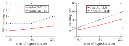
Refer to caption
Figure 8: AN and AL teaching costs for adaptive and non-adaptive teaching with increasing sizes of the hypothesis set in the robotic navigation scenario.

To test the advantage of adaptive teaching, we compare it with non-adaptive teaching in the presence of uncertainty. We consider local preferences with added uncertainty noises. Specifically, the learner has equal preference of selecting the formulas in the version space that have the least Manhattan distance from the current hypothesis and also any formula that can be perturbed from these formulas in the version space (here “perturb” means adding or subtracting the parameters i𝑖i or ϱ()italic-ϱ\varrho(\cdot) by 1).

Fig. 8 shows that Ada-AN-TLIP (i.e., adaptive AN-TLIP) can reduce the AN teaching costs by 28% compared with NAda-AN-TLIP (i.e., non-adaptive AN-TLIP), and Ada-AL-TLIP (i.e., adaptive AL-TLIP) can reduce the AN teaching costs by 30.75% compared with NAda-AL-TLIP (i.e., non-adaptive AL-TLIP).