Estimating heterogeneous treatment effects with right-censored data via causal survival forests

Abstract

Forest-based methods have recently gained in popularity for non-parametric treatment effect estimation. Building on this line of work, we introduce causal survival forests, which can be used to estimate heterogeneous treatment effects in a survival and observational setting where outcomes may be right-censored. Our approach relies on orthogonal estimating equations to robustly adjust for both censoring and selection effects under unconfoundedness. In our experiments, we find our approach to perform well relative to a number of baselines.

1 Introduction

The problem of heterogeneous treatment effect estimation plays a central role in data-driven personalization and, as such, has received considerable attention in the recent literature, including Athey and Imbens (2016), Foster and Syrgkanis (2019), Foster, Taylor, and Ruberg (2011), Hahn, Murray, and Carvalho (2017), Kennedy (2020), Künzel, Sekhon, Bickel, and Yu (2019), Luedtke and van der Laan (2016b), Nie and Wager (2021), Tian, Alizadeh, Gentles, and Tibshirani (2014) and Wager and Athey (2018). One difficulty in applying this line of work to medical applications, however, is that such applications often involve potentially censored survival outcomes—and existing methods for treatment heterogeneity often cannot be used in this setting.

To address this challenge, we propose causal survival forests, an adaptation of the causal forest algorithm of Athey, Tibshirani, and Wager (2019) that adjusts for censoring using doubly robust estimating equations developed in the survival analysis literature (Tsiatis, 2007; van der Laan and Robins, 2003). The method is robust, computationally tractable, and outperforms available baselines in our experiments. We also study the asymptotic behavior of causal survival forests, and establish conditions under which its predictions are consistent and asymptotically normal.

We focus on a statistical setting where, for $i=1,\,\ldots,\,n$ training examples, we assume independent and identically distributed (i.i.d.) tuples $\left\{X_{i},\,T_{i},\,C_{i},\,W_{i}\right\}$ where $X_{i}\in\mathcal{X}$ denote covariates, $T_{i}\in\mathbb{R}_{+}$ is the survival time for the $i$-th unit, $C_{i}\in\mathbb{R}_{+}$ is the time at which the $i$-th unit gets censored, and $W_{i}\in\left\{0,\,1\right\}$ denotes treatment assignment. The goal of a statistician is to measure the average effect of the treatment $W_{i}$ on survival time $T_{i}$ conditional on $X_{i}=x$. We define causal effects in terms of the standard potential outcomes framework (Imbens and Rubin, 2015), i.e., we posit potential outcomes $\left\{T_{i}(0),\,T_{i}(1)\right\}$ such that $T_{i}=T_{i}(W_{i})$, and seek to estimate the conditional average treatment effect on the survival time,

$$\tau(x)=\mathbb{E}\left[T_{i}(1)-T_{i}(0)\,\big{|}\,X_{i}=x\right],$$ (1)

or some relevant transformation of the survival time. However, unlike in the usual setting for heterogeneous treatment effect estimation discussed in, e.g., Künzel et al. (2019) and Nie and Wager (2021), we do not always get to see the realized survival time $T_{i}$; rather, we only observe $U_{i}=T_{i}\land C_{i}$ along with a non-censoring indicator $\Delta_{i}=1\left\{T_{i}\leq C_{i}\right\}$. The main challenge for causal survival forests is thus in estimating $\tau(x)$ in (1) while only observing $U_{i}$ and $\Delta_{i}$ as opposed to the target outcome $T_{i}$.

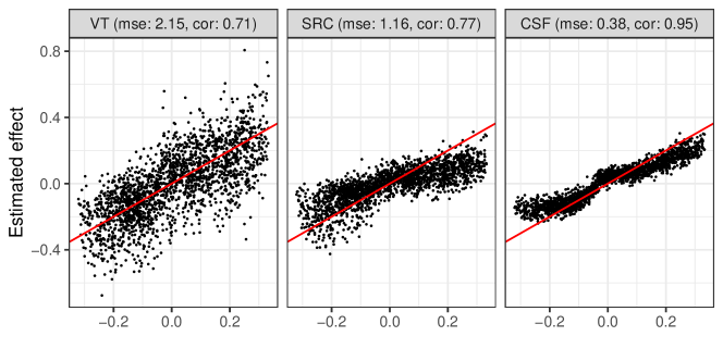
Figure 1: Conditional average treatment effect (CATE) predictions versus ground truth for the proposed method (“CSF”) with two alternatives, “VT”: virtual twins, “SRC”: the $S$-learner. The top row is for a data generating process with continuous survival time (the second kind described in section 4) and the bottom row for a data generating process with discrete response (the third kind described in section 4). Each estimator is fit on a sample size of 5 000, with default package tuning parameters (detailed in Section 4), predictions are for a test set of size 2 000. Mean squared error (MSE) and correlation with the true $\tau(x)$ is in parentheses. MSE is multiplied by 100 for readability.

To illustrate the promise of causal survival forests, consider the following simple simulation experiment. We compare our proposed method (CSF) to both an adaptation of the virtual twins method (VT) proposed by Foster, Taylor, and Ruberg (2011), and a variant of what Künzel et al. (2019) call the $S$-learner approach implemented using the survival forests from Ishwaran, Kogalur, Blackstone, and Lauer (2008) (SRC). We defer the details of these implementations to Section 4; however, we emphasize that—unlike our method—these baselines do not leverage insights from the literature on doubly robust survival analysis to target treatment effects. Moreover, following Athey and Imbens (2016), our method directly targets heterogeneity in the conditional average treatment effect when choosing where to place splits. In Figure 1 we plot estimated effects $\hat{\tau}(X_{i})$ against the true $\tau(X_{i})$ on randomly drawn test set points across two simulation designs discussed further in Section 4. In both cases, we find our approach to be considerably more accurate than the non-doubly robust baselines here.

Our paper is structured as follows. First, in Section 2, we motivate and present our proposed method, causal survival forests. In Section 3, we study asymptotics of causal survival forests in a generalized random forest setting introduced by Athey et al. (2019). In Section 4, we conduct simulation experiments, and find the proposed method to perform well in a wide variety of settings relative to other proposals in the literature. In Section 5, our approach is illustrated via a data application to the data from AIDS Clinical Trials Group Protocol 175 (ACTG175). A software implementation is provided as part of the package grf for R and C++, available from CRAN and at github.com/grf-labs/grf (Tibshirani et al., 2022; R Core Team, 2019)

1.1 Related work

As discussed above, there is an extensive recent literature on non-parametric methods for heterogeneous treatment effect estimation (Athey and Imbens, 2016; Athey et al., 2019; Foster et al., 2011; Friedberg et al., 2020; Hahn et al., 2017; Hill, 2011; Kennedy, 2020; Künzel et al., 2019; Lu et al., 2018; Luedtke and van der Laan, 2016b; Nie and Wager, 2021; Oprescu et al., 2019; Tian et al., 2014; Wager and Athey, 2018). However, right-censored survival data are frequently encountered in clinical trials and other biomedical research studies, and challenges related to this setting have mostly not been addressed in the existing literature. Here, we take a step towards enabling flexible heterogeneous treatment effect estimation with survival data by adapting the forest-based method of Athey et al. (2019) to this setting.

Random forests were originally proposed by Breiman (2001), and trace back to the work of Breiman et al. (1984) on CART trees. By now, the literature on general random forest methods for survival data has already received considerable attention; and in particular Leblanc and Crowley (1993) and Hothorn et al. (2006b) studied survival tree models in the context of conditional inference trees; Hothorn et al. (2006a) proposed using inverse probability of censoring weighting to compensate censoring in forest models; Ishwaran et al. (2008) proposed random survival forests, which extend random forests to handle survival data via using log-rank tests at each split on an individual survival tree (Ciampi et al., 1986; Segal, 1988); Zhu and Kosorok (2012) studied the impact of recursive imputation of survival forests on model fitting; Steingrimsson et al. (2016) proposed doubly robust survival trees by constructing doubly robust loss functions that use more information to improve efficiency; and Steingrimsson et al. (2019) constructed censoring unbiased regression trees and forests by considering a class of censoring unbiased loss functions. However, none of these methods were directly targeted at heterogeneous treatment effects in observational studies.

Finally, we note that the problem of heterogeneous treatment effect estimation is closely related to that of optimal treatment regimes or policy learning (Athey and Wager, 2021; Cui, 2021; Manski, 2004; Murphy, 2003; Qian and Murphy, 2011; Luedtke and van der Laan, 2016a; Zhang et al., 2012; Zhao et al., 2012). And, unlike in the case of heterogeneous treatment effects, there has been more work on developing methods for optimal treatment regimes under censoring. Adapting the outcome weighted learning framework (Zhao et al., 2012), Zhao et al. (2015) proposed two new approaches, inverse censoring weighted outcome weighted learning, and doubly robust outcome weighted learning, both of which require semi-parametric estimation of the conditional censoring probability given the patient characteristics and treatment choice. Zhu et al. (2017) adopted the accelerated failure time model to estimate an interpretable single-tree treatment decision rule. Cui et al. (2017) proposed a random forest approach for right-censored outcome weighted learning, which avoids both the inverse probability of censoring weighting and restrictive modeling assumptions. However, for observational studies with censored survival outcomes, these methods may suffer from confounding and selection bias. In addition, none of the above approaches focus on estimating the heterogeneous treatment effect or on associated uncertainty quantification.

2 Causal survival forests

As discussed above, our statistical setting is specified in terms of the distribution of i.i.d. tuples $\left\{X_{i},\,T_{i},\,C_{i},\,W_{i}\right\}\in\mathcal{X}\times\mathbb{R}_{+}\times\mathbb{R}_{+}\times\left\{0,\,1\right\}$, and we are interested in measuring the effect of a binary treatment $W$ on some deterministic transformation of the survival time $T$, i.e.,

$$\tau(x)=\mathbb{E}\left[y(T_{i}(1))-y(T_{i}(0))\,\big{|}\,X_{i}=x\right].$$ (2)

To streamline our presentation, with a slight abuse of notation, $\tau(x)$ is redefined as (2) hereafter. We observe censored survival times $U_{i}=T_{i}\land C_{i}$, and write the non-censoring indicator $\Delta_{i}=1\left\{T_{i}\leq C_{i}\right\}$.

Remark 1.

Note that (1) is a special case of (2) with $y(T)=T$. Other transformations include $y(T)=T\land h$ for the restricted mean survival time and $y(T)=1\left\{T\geq h\right\}$ for the survival probability.

Throughout, we will assume that the transformation $y(\cdot)$ is indifferent to survival beyond some maximal time horizon $h$. The reason we make this assumption is that, in most studies, all units are censored after some finite amount of time (e.g., in a 10-year study, no units will be observed past the 10-year mark), and functionals of $T_{i}$ that depend on behavior past this point will not be identified. The upshot of Assumption 1 is that we can treat any sample tracked past the horizon $h$ as “observed”, even if they are eventually censored.

Assumption 1.

(Finite horizon) The outcome transformation $y(\cdot)$ admits a maximal horizon $0<h<\infty$, such that $y(t)=y(h)$ for all $t\geq h$.

Definition 1.

(Effective non-censoring indicator) Under Assumption 1, we define the effective non-censoring indicator as $\Delta_{i}^{h}=1\left\{(T_{i}\land h)\leq C_{i}\right\}$; or, equivalently in terms of the observation $U_{i}$, we have $\Delta_{i}^{h}=\Delta_{i}\lor 1\left\{U_{i}\geq h\right\}$.

In order to identify treatment effects, we need to rely on two sets of assumptions. First, we need to make basic causal assumptions that would enable us to estimate the causal effect of $W_{i}$ on $T_{i}$ without censoring. The three assumptions below do so following Rosenbaum and Rubin (1983), and correspond exactly to standard assumptions used to identify the conditional average treatment effect (1) in the literature on heterogeneous treatment effect estimation (Künzel et al., 2019; Nie and Wager, 2021).

Assumption 2.

(Potential outcomes) There are potential outcomes $\left\{T_{i}(0),\,T_{i}(1)\right\}$ such that $T_{i}=T_{i}(W_{i})$ almost surely.

Assumption 3.

(Ignorability) Treatment assignment is as good as random conditionally on covariates, $\{T_{i}(0),T_{i}(1)\}\perp W_{i}\mid X_{i}$.

Assumption 4.

(Overlap) The propensity score $e(x)=\mathbb{P}\left[W_{i}=1\,\big{|}\,X_{i}=x\right]$ is uniformly bounded away from 0 and 1, i.e., $\eta_{e}\leq e(x)\leq 1-\eta_{e}$ for some $0<\eta_{e}\leq\frac{1}{2}$.

Second, we need assumptions to guarantee that censoring due to $C_{i}$ does not break identification results for treatment effects obtained via Assumptions 2–4. To this end, we rely on standard assumptions from survival analysis (e.g., Fleming and Harrington, 2011).

Assumption 5.

(Ignorable censoring) Censoring is independent of survival time conditionally on treatment and covariates, $T_{i}\mathchoice{\mathrel{\hbox to0.0pt{$\displaystyle\perp$\hss}\mkern 2.0mu{\displaystyle\perp}}}{\mathrel{\hbox to0.0pt{$\textstyle\perp$\hss}\mkern 2.0mu{\textstyle\perp}}}{\mathrel{\hbox to0.0pt{$\scriptstyle\perp$\hss}\mkern 2.0mu{\scriptstyle\perp}}}{\mathrel{\hbox to0.0pt{$\scriptscriptstyle\perp$\hss}\mkern 2.0mu{\scriptscriptstyle\perp}}}C_{i}\mid X_{i},\,W_{i}$.

Assumption 6.

(Positivity) $\mathbb{P}\left[C_{i}<h\,\big{|}\,X_{i},\,W_{i}\right]\leq 1-\eta_{C}$ for some $0<\eta_{C}\leq 1$.

Assumptions 5 and 6 play a fundamental role for identification. Qualitatively, we note that these two assumptions can be seen as direct analogues to Assumptions 3 and 4, where the former control how censoring due to $C_{i}$ can mask information about $T_{i}$ whereas the latter control how treatment assignment $W_{i}$ can mask information about the potential outcomes $\left\{T_{i}(0),\,T_{i}(1)\right\}$.

Below, we start by reviewing the causal forest algorithm of Athey et al. (2019) that can be used to estimate the conditional average treatment effect without censoring under Assumptions 2–4. Next, we discuss two adaptations of causal forests for censored survival data: First, in Section 2.2, we discuss a simple proposal based on inverse-probability of censoring weighting and then, in Section 2.3, we give our main proposal based on a doubly-robust censoring adjustment.

2.1 Causal forests without censoring

The basic causal forest algorithm is motivated by the following fact. If we knew that the treatment effects were constant, i.e., $\tau(x)=\tau$ for all $x$, then the following estimator $\hat{\tau}$ due to Robinson (1988) attains $1/\sqrt{n}$ rates of convergence, provided the three assumptions detailed above hold and that we estimate nuisance components sufficiently fast (Chernozhukov et al., 2018):

$$\begin{split}&\sum_{i=1}^{n}\psi^{(c)}_{\hat{\tau}}(X_{i},\,y(T_{i}),\,W_{i};\,\hat{e},\,\hat{m})=0,\\ &\psi^{(c)}_{\tau}(X_{i},\,y(T_{i}),\,W_{i};\,\hat{e},\,\hat{m})=\left[W_{i}-\hat{e}(X_{i})\right]\left[y(T_{i})-\hat{m}(X_{i})-\tau\left(W_{i}-\hat{e}(X_{i})\right)\right],\end{split}$$ (3)

where $e(x)=\mathbb{P}\left[W_{i}=1|X_{i}=x\right]$, $m(x)=\mathbb{E}\left[y(T_{i})|X_{i}=x\right]$, and $\hat{e}(X_{i})$ and $\hat{m}(X_{i})$ are estimates of these quantities derived via cross-fitting (Schick, 1986). We use the superscript $(c)$ to remind ourselves that this estimator requires access to the complete (uncensored) data.

Here, however, our goal is not to estimate a constant treatment effect $\tau$, but rather to fit covariate-dependent treatment heterogeneity $\tau(x)$; and we do so using a random forest method. As background, recall that given a target point $x$, tree-based methods seek to find training examples which are close to $x$ and use the local kernel weights to obtain a weighted averaging estimator. An essential ingredient of tree-based methods is recursive partitioning of the covariate space ${\pazocal X}$, which induces the local weighting. When the splitting variables are adaptively chosen, the width of a leaf can be narrower along the directions where the causal effect is changing faster. After the tree fitting is completed, the closest points to $x$ are those that fall into the same terminal node as $x$. The observations that fall into the same node as the target point $x$ can be treated asymptotically as coming from a homogeneous group.

Athey et al. (2019) generalizes the use of random forest-based weights for generic kernel estimation. The most closely related precedent from the perspective of adaptive nearest neighbor estimation are quantile regression forests (Meinshausen, 2006) and bagging survival trees (Hothorn et al., 2004), which can be viewed as special cases of generalized random forests. The idea of adaptive nearest neighbors also underlies theoretical analyses of random forests such as Arlot and Genuer (2014), Biau et al. (2008), and Lin and Jeon (2006). The random forest-based weights $\alpha_{i}$ are derived from the fraction of trees in which an observation appears in the same terminal node as the target point. Specifically, given a test point $x$, the weights $\alpha_{i}(x)$ are the frequency with which the $i$-th training example falls in the same leaf as $x$, i.e.,

$$\alpha_{i}(x)=\frac{1}{B}\sum_{b=1}^{B}\frac{1\left\{X_{i}\in{\pazocal N}_{b}(x)\right\}}{|{\pazocal N}_{b}(x)|},$$ (4)

where ${\pazocal N}_{b}(x)$ is the terminal node that contains $x$ in the $b$-th tree, $B$ is the number of trees, and $|\cdot|$ denotes the cardinality.

The crux of the causal forest algorithm presented in Athey et al. (2019) is to pair the kernel-based view of forests with Robinson’s estimating equation (3). Causal forests seek to grow a forest such that the resulting weighting function $\alpha_{i}(x)$ can be used to express heterogeneity in $\tau(\cdot)$, meaning that $\tau(\cdot)$ is roughly constant over observations given positive weight $\alpha_{i}(x)$ for predicting at $x$. Then, we estimate $\tau(x)$ by solving a localized version of (3):

$$\sum_{i=1}^{n}\alpha_{i}(x)\psi^{(c)}_{\hat{\tau}(x)}(X_{i},\,y(T_{i}),\,W_{i};\,\hat{e},\,\hat{m})=0.$$ (5)

Athey et al. (2019) discuss additional details including the choice of a splitting rule targeted for treatment heterogeneity, while Nie and Wager (2021) and Kennedy (2020) further explore the idea of using Robinson’s transformation to fit treatment heterogeneity. For a general review and discussion of causal forests, see Athey and Wager (2019).

2.2 Adjusting for censoring via weighting

In the presence of censoring, the estimator (5) is no longer applicable because $T_{i}$ is not always observed. Simply ignoring censoring and running causal forests with complete observations (i.e., those with $\Delta_{i}^{h}=1$) would lead to bias. However, under Assumptions 5 and 6, several general approaches for making statistical estimators robust to censoring are available.

One particularly simple censoring adjustment is via inverse-probability of censoring weighting (IPCW). Let

$$S_{w}^{C}(s|x)=\mathbb{P}\left[C_{i}\geq s|W_{i}=w,X_{i}=x\right]$$ (6)

denote the conditional survival function for the censoring process, and note that any given survival time is observed in the sense of Definition 1 with probability

$$\mathbb{P}\left[\Delta_{i}^{h}=1\,\big{|}\,X_{i},\,W_{i},\,T_{i}\right]=S_{W_{i}}^{C}\left(T_{i}\land h\,\big{|}\,X_{i}\right),$$ (7)

The main idea of IPCW estimation is to only consider complete cases, but up-weight all complete observations by $1/S_{W_{i}}^{C}\left(T_{i}\land h\,\big{|}\,X_{i}\right)$ to compensate for censoring. As discussed in van der Laan and Robins (2003, Chapter 3.3), such IPCW estimators succeed in eliminating censoring bias under considerable generality.

In the context of causal forests, IPCW estimation for an outcome transformation satisfying Assumption 1 amounts to estimating $\tau(x)$ as

$$\sum_{\left\{i:\Delta_{i}^{h}=1\right\}}\frac{\alpha_{i}(x)}{\hat{S}_{W_{i}}^{C}\left(T_{i}\land h\,\big{|}\,X_{i}\right)}\psi^{(c)}_{\hat{\tau}(x)}(X_{i},\,y(T_{i}),\,W_{i};\,\hat{e},\,\hat{m})=0,$$ (8)

where $\hat{S}_{w}^{C}(s|x)$ is an estimate of (6) that’s pre-computed using cross-fitting just like $\hat{e}$ and $\hat{m}$, and $\alpha_{i}(x)$ is obtained as in (4) trained on complete observations only. This algorithm forms a first adaptation of causal forests for censored data. We note that, when using (8), the nuisance component $\hat{m}(x)$ also needs to be estimated in a way that accounts for censoring; here, the IPCW approach can again be used. Concretely, we implement IPCW causal forests by training a model on samples with observed failure times only $(\Delta_{i}^{h}=1)$, and pass $1/\hat{S}_{W_{i}}^{C}\left(T_{i}\land h\,\big{|}\,X_{i}\right)$ as a “sample weight” to the function causal_forest in grf (Tibshirani et al., 2022). We refer to the grf package documentation for more details of how sample weights are incorporated in all parts of the algorithm (including in splitting).

2.3 A doubly robust correction

While the IPCW approach discussed above is attractive in terms of its simplicity, it has several statistical drawbacks. First, this estimation strategy requires us to effectively throw away all observations with $\Delta_{i}^{h}=0$, and this may hurt us in terms of efficiency: After all, if we see that a sample got censored at time $U_{i}>0$, then at least we know they didn’t die before $U_{i}$, and a powerful estimation procedure should be able to take this into account. Second, in general, we need to run IPCW with an estimate of $\hat{S}_{w}^{C}(s|x)$, and IPCW-type methods are generally not robust to estimation errors in this quantity—which will be a problem especially if we want to use flexible methods like random survival forests for estimating $\hat{S}_{w}^{C}(s|x)$ (Chernozhukov et al., 2018; van der Laan and Rose, 2011).

For this reason, our preferred causal survival forest method does not rely on IPCW, and instead relies on a more robust approach to making estimating equations robust to censoring, described in Tsiatis (2007, Chapter 10.4). If the true value $\tau$ of our parameter of interest is identified by a complete data estimating equation, $\mathbb{E}[\psi_{\tau}^{(c)}(X_{i},\,y(T_{i}),\,W_{i})]=0$ then, under Assumption 1, $\tau$ is also identified via the following estimator that generalizes the celebrated augmented inverse-propensity weighting estimator of Robins et al. (1994). We have $\mathbb{E}\left[\psi_{\tau}(X_{i},\,y(U_{i}),\,U_{i}\land h,\,W_{i},\,\Delta_{i}^{h})\right]=0$ with scores

$$\begin{split}&\psi_{\tau}(X_{i},\,y(U_{i}),\,U_{i}\land h,\,W_{i},\,\Delta_{i}^{h})=\frac{\Delta_{i}^{h}\,\psi_{\tau}^{(c)}(X_{i},\,y(U_{i}),\,W_{i})}{S_{W_{i}}^{C}(U_{i}\land h|X_{i})}\\ &\ \ \ \ \ \ \ \ +\frac{(1-\Delta_{i}^{h})\mathbb{E}\left[\psi_{\tau}^{(c)}(X_{i},\,y(T_{i}),\,W_{i})|T_{i}\land h>U_{i}\land h,\,W_{i},\,X_{i}\right]}{S_{W_{i}}^{C}(U_{i}\land h|X_{i})}\\ &\ \ \ \ \ \ \ \ -\int_{0}^{U_{i}\land h}\frac{\lambda_{W_{i}}^{C}(s|X_{i})}{S_{W_{i}}^{C}(s|X_{i})}\mathbb{E}\left[\psi_{\tau}^{(c)}(X_{i},\,y(T_{i}),\,W_{i})|T_{i}\land h>s,\,W_{i},\,X_{i}\right]\ ds,\end{split}$$ (9)

where $S_{w}^{C}(s|x)$ is the conditional survival function as defined in (6) and

$$\lambda_{w}^{C}(s|x)=-\frac{d}{ds}\log S_{w}^{C}(s|x)$$ (10)

is the associated conditional hazard function.

When applied to the complete data estimating equation (3) used to motivate causal forests, this approach gives us scores

$$\begin{split}&\psi_{\tau}(X_{i},\,y(U_{i}),\,U_{i}\land h,\,W_{i},\,\Delta_{i}^{h};\,\hat{e},\,\hat{m},\,\hat{\lambda}^{C}_{w},\,\hat{S}^{C}_{w},\,\hat{Q}_{w})\\ &\ \ \ =\bigg{(}\frac{\hat{Q}_{W_{i}}(U_{i}\land h|X_{i})+\Delta_{i}^{h}[y(U_{i})-\hat{Q}_{W_{i}}(U_{i}\land h|X_{i})]-\hat{m}(X_{i})-\tau\left(W_{i}-\hat{e}(X_{i})\right)}{\hat{S}_{W_{i}}^{C}(U_{i}\land h|X_{i})}\\ &\ \ \ \ \ \ -\int_{0}^{U_{i}\land h}\frac{\hat{\lambda}_{W_{i}}^{C}(s|X_{i})}{\hat{S}_{W_{i}}^{C}(s|X_{i})}[\hat{Q}_{W_{i}}(s|X_{i})-\hat{m}(X_{i})-\tau\left(W_{i}-\hat{e}(X_{i})\right)]\ ds\bigg{)}\left(W_{i}-\hat{e}(X_{i})\right),\end{split}$$ (11)

where $Q_{w}(s|x)=\mathbb{E}\left[y(T_{i})\,\big{|}\,X_{i}=x,\,W_{i}=w,\,T_{i}\land h>s\right]$ is the conditional expectation of the transformed survival time, while $\hat{Q}_{w}(s|x)$, $\hat{S}_{w}^{C}(s|x)$ and $\hat{\lambda}_{w}^{C}(s|x)$ are cross-fit nuisance parameter estimates. For example, $\hat{Q}_{w}(s|x)$ can be estimated by an integral of estimated survival functions and $\hat{\lambda}_{w}^{C}(s|x)$ can be estimated as a forward difference of $-\log(\hat{S}_{w}^{C}(s|x))$.

The standard way of using scores is to construct a Neyman-orthogonal robust estimator of a relevant global parameter; see Chernozhukov et al. (2018) for a general discussion and references. In our case, the scores (11) induce a robust estimator $\hat{\tau}$ for a global constant treatment effect parameter $\tau$:

$$\sum_{i=1}^{n}\psi_{\hat{\tau}}(X_{i},\,y(U_{i}),\,U_{i}\land h,\,W_{i},\,\Delta_{i}^{h};\,\hat{e},\,\hat{m},\,\hat{\lambda}^{C}_{w},\,\hat{S}^{C}_{w},\,\hat{Q}_{w})=0.$$ (12)

This estimator is Neyman-orthogonal in the sense discussed in Chernozhukov et al. (2018), and attains a $1/\sqrt{n}$ rate of convergence for $\tau$ under 4-th root rates for the nuisance components, provided we use cross-fitting and that Assumptions 2–6 hold. Then the following result, given here for reference, illustrates the type of results one can get from this approach. The proof follows from arguments made in Chernozhukov et al. (2018) and Tsiatis (2007); see also van der Laan and Robins (2003) for an extensive discussion of double robustness under right-censoring.

Proposition 1.

Assume that the conditional average treatment effects are constant, $\tau(x)=\tau$ for all $x\in{\pazocal X}$, and let $\tilde{\tau}$ be an oracle estimator for $\tau$, i.e., the solution to equation  (12) with estimated nuisance components $\hat{e},\,\hat{m},\,\hat{\lambda}^{C}_{w}/\hat{S}^{C}_{w},\,\hat{S}^{C}_{w},\,\hat{Q}_{w}$ replaced by true values for ${e},\,{m},\,{\lambda}^{C}_{w}/{S}^{C}_{w},\,{S}^{C}_{w},\,{Q}_{w}$. Suppose $\sup_{x\in{\pazocal X}}|\hat{e}(x)-e(x)|=o_{p}(1)$, $\sup_{x\in{\pazocal X}}|\hat{m}(x)-m(x)|=o_{p}(1)$, and $\sup_{x\in{\pazocal X},s\leq h}|\hat{S}^{C}_{w}(s|x)-S^{C}_{w}(s|x)|=o_{p}(1)$, $\sup_{x\in{\pazocal X},s\leq h}|\hat{Q}_{w}(s|x)-Q_{w}(s|x)|=o_{p}(1)$, $\sup_{x\in{\pazocal X},s\leq h}|\frac{\hat{\lambda}^{C}_{w}(s|x)}{\hat{S}^{C}_{w}(s|x)}-\frac{\lambda^{C}_{w}(s|x)}{S^{C}_{w}(s|x)}|=o_{p}(1)$ for both $w=0,1$. In addition, we assume that $\mathbb{E}\left[|\hat{e}(X)-e(X)|^{2}\right]=o(b_{n}^{2})$, $\mathbb{E}\left[|\hat{m}(X)-m(X)|^{2}\right]=o(c_{n}^{2})$, and $\sup_{s\leq h}\mathbb{E}\left[|\hat{S}^{C}_{w}(s|X)-S^{C}_{w}(s|X)|^{2}\right]=o(c_{n}^{2})$, $\sup_{s\leq h}\mathbb{E}\left[|\hat{Q}_{w}(s|X)-Q_{w}(s|X)|^{2}\right]=o(c_{n}^{2})$, $\sup_{s\leq h}\mathbb{E}\left[|\frac{\hat{\lambda}^{C}_{w}(s|X)}{\hat{S}^{C}_{w}(s|X)}-\frac{\lambda^{C}_{w}(s|X)}{S^{C}_{w}(s|X)}|^{2}\right]=o(d_{n}^{2})$ for both $w=0,1$. Then, provided Assumptions 2–6 hold, we have $\hat{\tau}-\tilde{\tau}=o_{p}(\max((c_{n}+d_{n})c_{n},b_{n}c_{n},b^{2}_{n}))$. Furthermore, the solution $\hat{\tau}$ to estimating equation  (12) has an asymptotically normal sampling distribution and attains a $1/\sqrt{n}$ rate of convergence, provided the nuisance components $\hat{e},\,\hat{m},\,\hat{\lambda}^{C}_{w}/\hat{S}^{C}_{w},\,\hat{S}^{C}_{w},\,\hat{Q}_{w}$ are learned using cross-fitting, are uniformly consistent and achieve 4-th root rates of convergence in root-mean squared error.

Our causal survival forests also use the doubly robust scores (11), but now in the context of a forest-based estimator for treatment heterogeneity. First, we estimate the nuisance components $\hat{e},\,\hat{m},\,\hat{\lambda}^{C}_{w},\,\hat{S}^{C}_{w},\,\hat{Q}_{w}$ required to form the score (11), and then pair this estimating equation with the forest weighting scheme (5), resulting in estimates $\hat{\tau}(x)$ characterized by

$$\sum_{i=1}^{n}\alpha_{i}(x)\psi_{\hat{\tau}(x)}(X_{i},\,y(U_{i}),\,U_{i}\land h,\,W_{i},\,\Delta_{i}^{h};\,\hat{e},\,\hat{m},\,\hat{\lambda}^{C}_{w},\,\hat{S}^{C}_{w},\,\hat{Q}_{w})=0.$$ (13)

In order to use this estimator, we of course need to specify how to grow the forest, so that the resulting forest weights $\alpha_{i}(x)$ adequately express heterogeneity in the underlying signal $\tau(x)$. Here, for the splitting rule, we use the $\widetilde{\Delta}$-criterion proposed in Athey et al. (2019). In particular, we generate pseudo-outcomes by the following relabeling strategy at each parent node ${\pazocal N}$,

$$\rho_{i}=\psi^{i}_{\hat{\tau}_{\pazocal N}}\times\left[\frac{1}{|\{j:X_{j}\in{\pazocal N}\}|}\sum_{j:X_{j}\in{\pazocal N}}(W_{j}-\hat{e}(X_{j}))^{2}\left(\frac{1}{\hat{S}^{C}_{W_{j}}(U_{j}\land h|X_{j})}-\int_{0}^{U_{j}\land h}\frac{\hat{\lambda}_{W_{j}}^{C}(s|X_{j})}{\hat{S}^{C}_{W_{j}}(s|X_{j})}ds\right)\right]^{-1},$$ (14)

where $\psi^{i}_{\hat{\tau}_{\pazocal N}}$ is a shorthand of $\psi_{\hat{\tau}_{\pazocal N}}(X_{i},\,y(U_{i}),\,U_{i}\land h,\,W_{i},\,\Delta_{i}^{h};\,\hat{e},\,\hat{m},\,\hat{\lambda}^{C}_{w},\,\hat{S}^{C}_{w},\,\hat{Q}_{w})$, and $\hat{\tau}_{\pazocal N}$ is the estimated $\tau$ in ${\pazocal N}$ by (12). Next, the splitting criterion proceeds exactly the same as a regression tree (Breiman et al., 1984) problem by treating the pseudo-outcomes $\rho_{i}$’s as a continuous outcome variable. Specifically, we split the parent node into two child nodes ${\pazocal N}_{L}$ and ${\pazocal N}_{R}$ so as to maximize the following quantity:

$$\widetilde{\Delta}(L,R)=\frac{1}{|\{i:X_{i}\in{\pazocal N}_{L}\}|}\Bigg{(}\sum_{i:X_{i}\in{\pazocal N}_{L}}\rho_{i}\Bigg{)}^{2}+\frac{1}{|\{i:X_{i}\in{\pazocal N}_{R}\}|}\Bigg{(}\sum_{i:X_{i}\in{\pazocal N}_{R}}\rho_{i}\Bigg{)}^{2}.$$

Remark 2.

Throughout this paper, we will present our method and formal results in a general setting that covers any outcome transformation $y(\cdot)$ satisfying Assumption 1. However, the implementation of our doubly robust method, provided as the causal_survival_forest function in grf, only considers two target outcomes: The restricted mean survival time (RMST),

$$\tau^{h}(x)=\mathbb{E}\left[T_{i}(1)\land h\,\big{|}\,X_{i}=x\right]-\mathbb{E}\left[T_{i}(0)\land h\,\big{|}\,X_{i}=x\right],$$ (15)

which arises from our framework using $y(T)=T\land h$, and the survival probability,

$$\pi^{h}(x)=\mathbb{P}\left[T_{i}(1)\geq h\,\big{|}\,X_{i}=x\right]-\mathbb{P}\left[T_{i}(0)\geq h\,\big{|}\,X_{i}=x\right],$$ (16)

which arises from using $y(T)=1\left\{T\geq h\right\}$. Methodological extensions to other outcome transformations is straightforward, but requires modifying estimators for the nuisance components $\hat{Q}_{w}(s|x)$ and $\hat{m}(x)$. In our implementation for estimating $\tau^{h}(x)$ and $\pi^{h}(x)$, $\hat{Q}_{w}(s|x)$ and $\hat{m}(x)$ are derived from the estimated conditional survival function of the survival time.

Remark 3.

Our splitting rule based on pseudo-outcomes as in (14) is a direct application of the abstract GRF-algorithm of Athey et al. (2019). This algorithmic technique is motivated by classical influence-function based approximations for semiparametric inference (Andrews, 1993; Zeileis, 2005). An alternative approach to splitting that could also be used with our doubly robust estimating equation is to maximize a test statistic for treatment heterogeneity as in, e.g., Zeileis et al. (2008) or Yang et al. (2021). Athey et al. (2019) have a further discussion of both statistical and computational properties of pseudo-outcome-based splitting.

3 Asymptotics and inference

A main draw of forest based methods is that they have repeatedly proven themselves to be both robust and flexible in practice. However, to further our statistical understanding of the method, it is helpful to study the behavior of the method under a more restricted asymptotic setting where sharp formal characterizations are available. To this end, we now study asymptotics of causal survival forests in a setting that builds on the one used by Wager and Athey (2018) to study inference with forests in problems without censoring. Throughout this section, we assume that the covariates $X\in{\pazocal X}=[0,1]^{p}$ are distributed according to a density that is bounded away from zero and infinity. The following assumption guarantees the smoothness of $\mathbb{E}\left[\psi_{\tau(x)}|X=x\right]$.

Assumption 7.

(Lipschitz continuity) The treatment effect function $\tau(x)$ is Lipschitz continuous in terms of $x$. In addition, the nuisance components $e(x)$, $m(x)$ are Lipschitz continuous in terms of $x$, and $Q_{w}(s|x)$, $\lambda_{w}^{C}(s|x)$, $S_{w}^{C}(s|x)$ are Lipschitz continuous in terms of $x$ for both $w\in\{0,1\}$ and all $s\leq h$.

In addition, our trees are symmetric, i.e., their output is invariant to permuting the indices of training samples. Our algorithm also guarantees honesty (Wager and Athey, 2018), and the following two conditions.

Random split tree: At each internal node, the probability of splitting at the $j$-th dimension is greater than $\varsigma$, where $0<\varsigma<1$ for $j=1,\ldots,p$.

Subsampling: Each child node contains at least a fraction $\nu$ of the data points in its parent node for some $0<\nu<0.5$, and trees are grown on subsamples of size $\ell$ scaling as

$$\ell=n^{\gamma},\ \ \ \ \kappa<\gamma<1,\ \ \ \ \kappa\equiv 1-\big{[}1+\varsigma^{-1}\big{(}\log(\nu^{-1})\big{)}/\big{(}\log(1-\nu)^{-1}\big{)}\big{]}^{-1}.$$ (17)

We note that, in Theorem 3, we will obtain a rate of convergence of $\widetilde{O}(\sqrt{\ell/n})$ for $\hat{\tau}(x)$, where $\widetilde{O}(\cdot)$ denotes the term neglecting the logarithmic factors; thus (17) captures the asymptotic behavior we can get; see Wager and Athey (2018) for an in-depth discussion of this assumption.

Moreover, we need Assumption 8 to couple $\hat{\tau}(x)$ and $\tilde{\tau}(x)$, where $\tilde{\tau}(x)$ is an oracle estimator, with nuisance components ${e},\,{m},\,{\lambda}^{C}_{w},\,{S}^{C}_{w},\,{Q}_{w}$ being the underlying truth instead of their empirical analogues in equation (11).

Assumption 8.

Consistency of the non-parametric plug-in estimators: we have the following convergences in probability,

$$\sup_{x\in{\pazocal X}}|\hat{e}(x)-e(x)|\rightarrow 0,~{}\sup_{x\in{\pazocal X}}|\hat{m}(x)-m(x)|\rightarrow 0,$$

and

$$\sup_{x\in{\pazocal X},s\leq h}|\hat{S}^{C}_{w}(s|x)-S^{C}_{w}(s|x)|\rightarrow 0,\sup_{x\in{\pazocal X},s\leq h}|\hat{Q}_{w}(s|x)-Q_{w}(s|x)|\rightarrow 0,\sup_{x\in{\pazocal X},s\leq h}|\frac{\hat{\lambda}^{C}_{w}(s|x)}{\hat{S}^{C}_{w}(s|x)}-\frac{\lambda^{C}_{w}(s|x)}{S^{C}_{w}(s|x)}|\rightarrow 0,$$

for both $w=0,1$. Furthermore, suppose that

$$\mathbb{E}\left[\sup_{x\in{\pazocal X}}|\hat{e}(x)-e(x)|^{2}\right]=o(b_{n}^{2}),~{}\mathbb{E}\left[\sup_{x\in{\pazocal X}}|\hat{m}(x)-m(x)|^{2}\right]=o(c_{n}^{2}),$$

and

$$\sup_{s\leq h}\mathbb{E}\left[\sup_{x\in{\pazocal X}}|\hat{S}^{C}_{w}(s|x)-S^{C}_{w}(s|x)|^{2}\right]=o(c_{n}^{2}),$$ (18)

$$\sup_{s\leq h}\mathbb{E}\left[\sup_{x\in{\pazocal X}}|\hat{Q}_{w}(s|x)-Q_{w}(s|x)|^{2}\right]=o(c_{n}^{2}),$$ (19)

$$\sup_{s\leq h}\mathbb{E}\left[\sup_{x\in{\pazocal X}}|\frac{\hat{\lambda}^{C}_{w}(s|x)}{\hat{S}^{C}_{w}(s|x)}-\frac{\lambda^{C}_{w}(s|x)}{S^{C}_{w}(s|x)}|^{2}\right]=o(d_{n}^{2})$$ (20)

for both $w=0,1$.

Equations (18)-(20) imply the corresponding rate assumptions of Proposition 1. Assumption 8 is quite general and can be achieved by many existing models. Biau (2012); Wager and Walther (2015) show that for the random forest models, $b_{n}^{2}$ can be faster than $n^{-2/(p+2)}$ as long as the intrinsic signal dimension is less than $0.54p$. As shown in Cui et al. (2022), $c_{n}^{2}=n^{-1/(p+2)}$ is achievable for survival forest models. Non-parametric kernel smoothing methods such as Sun et al. (2019) provide estimation with $d_{n}^{2}=n^{-1/2+\kappa}$, where $\kappa<1/2$ depending on the dimension $p$.

The following lemma provides an intermediate result for our main theorem, which bounds the difference between $\hat{\tau}(x)$ and $\tilde{\tau}(x)$.

Lemma 2.

We assume Assumptions 6 and 8 hold. Then for any $x\in{\pazocal X}$, we have that $\hat{\tau}(x)-\tilde{\tau}(x)=o_{p}(\max((c_{n}+d_{n})c_{n},b_{n}c_{n},b^{2}_{n}))$.

The proof of Lemma 2 is deferred to the Appendix. The technical results in Wager and Athey (2018); Athey et al. (2019) paired with Lemma 2 lead to the following asymptotic Gaussianity result.

Theorem 3.

Assume Assumptions 2–8 hold, and that $\ell$ scales as in (17). If $o_{p}(\max((c_{n}+d_{n})c_{n},b_{n}c_{n},b^{2}_{n}))$ converges to zero with a faster rate than $polylog(n/\ell)^{-1/2}(\ell/n)^{1/2}$, where $polylog(n/\ell)$ is a function that is bounded away from 0 and increases at most polynomially with the log-inverse sampling ratio $\log(n/\ell)$. Then there exists a sequence $\sigma_{n}(x)$ such that for any $x\in{\pazocal X}$,

$$[\hat{\tau}(x)-\tau(x)]/\sigma_{n}(x)\rightarrow N(0,1),$$ (21)

where $\sigma^{2}_{n}(x)=polylog(n/\ell)^{-1}\ell/n$.

The proof of Theorem 3 is deferred to the Appendix. This asymptotic Gaussianity result yields valid asymptotic confidence intervals for the true treatment effect $\tau(x)$.

3.1 Pointwise confidence intervals

One important consequence of Theorem 3 is that, in settings where its assumptions hold, we can use (21) to build pointwise confidence intervals for $\tau(x)$: All we need for confidence intervals is a consistent estimator for the asymptotic variance of $\hat{\tau}(x)$. We proceed using the “bootstrap of little bags” algorithm (Athey, Tibshirani, and Wager, 2019; Sexton and Laake, 2009). The main idea of the bootstrap of little bags is to introduce some cluster structure into the random samples used by the random forest to grow each tree, and then use within vs between-cluster correlations in the behaviors of individual trees to reason about what we would have gotten by running (computationally infeasible) bootstrap uncertainty quantification on the whole forest.

Now, following the line of argument in Section 4 from Athey et al. (2019), under the conditions of Theorem 3 our estimator $\hat{\tau}(x)$ is asymptotically equivalent to

$$\tilde{\tau}^{*}(x)=\tau(x)+\sum_{i=1}^{n}\alpha_{i}(x)\rho_{i}^{*}(x),$$ (22)

where $\rho_{i}^{*}(x)$ is the influence function of the $i$-th observation with respect to the true parameter value $\tau(x)$, i.e., $\rho_{i}^{*}(x)=\psi^{i}_{\tau(x)}V(x)^{-1}$ with

$$V(x)=\mathbb{E}\left[\left(W-e(X)\right)^{2}\left(\frac{1}{S^{C}_{W}(U\land h|X)}-\int_{0}^{U\land h}\frac{\lambda_{W}^{C}(s|X)}{S^{C}_{W}(s|X)}ds\right)\bigg{|}X=x\right].$$ (23)

It thus follows that, to build confidence intervals, it suffices to estimate

$$\sigma_{n}^{2}(x)=\operatorname{Var}\left[\tilde{\tau}^{*}(x)\right]=\operatorname{Var}\left[\sum_{i=1}^{n}\alpha_{i}(x)\psi^{i}_{\tau(x)}\right]V(x)^{-2},$$ (24)

where we note $\sum_{i=1}^{n}\alpha_{i}(x)\psi^{i}_{\tau(x)}$ is formally equivalent to the prediction made by a regression forest with “outcome” $\psi^{i}_{\tau(x)}$. To this end, we set

$$\hat{\sigma}_{n}^{2}=\hat{H}_{n}(x)\hat{V}_{n}(x)^{-2},$$ (25)

where $\hat{H}_{n}(x)$ is estimated via the bootstrap of little bags device described above, and $\hat{V}_{n}(x)$ is a sample-version of (23) with forest-weights $\alpha_{i}(x)$. We refer to Section 4 of Athey et al. (2019) for further details and discussion of this approach.

3.2 Inference on linear projections of the CATE

The pointwise confidence intervals discussed above provide a valuable method for assessing the stability of causal survival forests, and also can be helpful in getting a handle on the behavior of $\tau(x)$ in large samples. However, using these estimates in practice can sometimes lead to difficulties. First, the problem of pointwise non-parametric inference of $\tau(x)$ is fundamentally a very difficult problem as the function $\tau(\cdot)$ may take on complex shapes (Chernozhukov et al., 2018; Imai and Li, 2019), which means that intervals for $\tau(x)$ will in general be quite wide. Second, the result (21) relies on the forest being tuned for “undersmoothing”, i.e., that errors of the forest are dominated by variance and bias is negligible. In practice, it can be difficult to detect cases where undersmoothing does not hold (and confidence intervals are centered on potentially biased point-estimates); see Appendix C3 of Athey et al. (2019) for further discussion.

In order to get around these difficulties, Semenova and Chernozhukov (2021) advocate focusing inference on low-dimensional summaries of $\tau(\cdot)$, including projections (Beran, 1977; White, 1980, 1982; Buja et al., 2019); see also van der Laan (2006) and Neugebauer and van der Laan (2007). Given a set of covariates $A_{i}$, the best linear projection of the CATE function $\tau(\cdot)$ is

$$\left\{\beta^{*}_{0},\,\beta^{*}\right\}=\operatorname{argmin}_{\beta_{0},\beta}\mathbb{E}\left[\left(\tau(X_{i})-\beta_{0}-A_{i}\beta\right)^{2}\right].$$ (26)

Typically, the $A_{i}$ will be chosen as a subset (or transformations) of the $X_{i}$. As argued in Semenova and Chernozhukov (2021), such linear projections can be used to meaningfully interpret and summarize treatment heterogeneity, but remain simple enough that we can still provide robust inference for them using well-understood techniques from the literature on semiparametrics. This means a researcher is able to pre-specify a hypothesis of how they believe the conditional mean of $\tau(X)$ varies with for example age and gender, and achieve valid inference for this association measure, even though point estimates of $\tau(X)$ may be quite uncertain and obtained non-parametrically.

To implement this approach, we first construct relevant doubly robust scores, based on the augmented inverse propensity weighting (Robins et al., 1994)

$$\widehat{\Gamma}_{i}=\hat{\tau}(X_{i})+\frac{\psi_{\hat{\tau}(X_{i})}(X_{i},\,y(U_{i}),\,U_{i}\land h,\,W_{i},\,\Delta_{i}^{h})}{\hat{e}(X_{i})(1-\hat{e}(X_{i}))},$$ (27)

where $\psi_{\tau}(\cdot)$ is as in (11) and $\hat{\tau}(X_{i})$ are CATE estimates provided by the causal survival forest. We then estimate the best linear projection (BLP) parameters (26) by running a linear regression of $\widehat{\Gamma}_{i}$ on the features of interest $A_{i}$; i.e., the regression $\widehat{\Gamma}_{i}\sim A_{i}$. Confidence intervals can be derived via any misspecification- and heteroskedasticity-robust approach to inference with ordinary least squares; in our implementation, we use the sandwich variance estimator with $HC_{3}$ covariance weights following MacKinnon and White (1985).

Semenova and Chernozhukov (2021) show that this approach yields a $\sqrt{n}$-rate central limit theorem for $\beta$ and $\beta_{0}$ under conditions analogous to those of Proposition 1 on the nuisance components. In the case of our forest-based approach, the rates of convergence for nuisance components may be slower than those required by the result of Semenova and Chernozhukov (2021) so we cannot formally verify that a $\sqrt{n}$-rate central limit theorem holds for us; however, as shown in our simulation experiments (see Figure 2), the estimator of Semenova and Chernozhukov (2021) has a very nearly normal sampling distribution.

Remark 4.

It would also be possible to consider the pseudo-outcomes from (27) as left-hand-side variables for non-parametric regression, thus providing an alternative starting point for non-parametric estimation of CATE with survival outcomes. This class of approaches has received considerable attention in recent years; see, e.g., Fan et al. (2022), Kennedy (2020) and Zimmert and Lechner (2019). Meanwhile, another alternative to best linear projections is to apply assumption-lean inference recently proposed by Vansteelandt and Dukes (2022) who use non-parametric projection to assess associations of the CATE with one variable at a time. Vansteelandt and Dukes (2022) argue that this approach provides robust summaries of the CATE when $\tau(\cdot)$ is non-linear in terms of the summarizing variables $A_{i}$.

4 Simulation study

We now turn to a simulation study to assess the empirical performance of causal survival forests. As discussed in Remark 2, given a target horizon $h$, we focus on estimating the effect of the treatment on both the restricted mean survival time at $h$ and on survival probability at $h$. The choice of horizon $h$ is given in each simulation specification.

In our experiments, we compare the following methods. (1) An adaptation of the virtual twin (VT) method of Foster et al. (2011) to survival data, using random survival forests as implemented in the package randomForestSRC (Ishwaran and Kogalur, 2019): We train two random survival forests, the first using the observations in the control group $\{(X,\,U,\,\Delta)\}_{W=0}$ to estimate $\mu_{0}(x)=\mathbb{E}\left[y(T_{i})\,\big{|}\,X_{i}=x,\,W_{i}=0\right]$, and the second using the observations in the treated group to estimate $\mu_{1}(x)=\mathbb{E}\left[y(T_{i})\,\big{|}\,X_{i}=x,\,W_{i}=1\right]$, where the conditional expectation estimation is constructed from the estimated conditional survival function, and then report $\hat{\tau}(x)=\hat{\mu}_{1}(x)-\hat{\mu}_{0}(x)$. (2) An instantiation of the $S$-learner strategy discussed in Künzel et al. (2019) using random survival forests (SRC1) as implemented in the package randomForestSRC: We train a single random survival forest with features $(X,\,W)$ to estimate $\mu(x,\,w)=\mathbb{E}\left[y(T_{i})\,\big{|}\,X_{i}=x,\,W_{i}=w\right]$, where the conditional expectation estimation is constructed from the estimated conditional survival function, and then report $\hat{\tau}(x)=\hat{\mu}(x,\,1)-\hat{\mu}(x,\,0)$. (3) Enriched random survival forests (SRC2) derived as above, except we train the forest with additional interaction features, i.e., $(X,\,W,\,XW)$ as considered in Lu et al. (2018). (4) Inverse-propensity of censoring weighted (IPCW) causal forests, as described in Section 2.2. (5) Our proposed causal survival forests (CSF), as described in Section 2.3. Both of our methods, IPCW and CSF, are run using publicly available implementations in the R package grf version 2.1, available from CRAN and at github.com/grf-labs/grf (Tibshirani et al., 2022; R Core Team, 2019).

We run the above methods on the following simulation designs. In each, we generated independent covariates from a uniform distribution on $[0,1]^{p}$ with $p=15$. We consider two estimands, the restricted mean survival time (RMST) and survival probability. For the first estimand, the truncation time is listed in the simulation settings; for the second estimand, we consider surviving past the 90-th percentile of $U$. The Supplementary Material shows results when the covariates have a non-diagonal covariance matrix $V$ with entries $V_{ij}=0.5^{|i-j|}$.

Setting 1. We generate $T$ from an accelerated failure time model, and $C$ from a Cox model,

$$\log({T})=-1.85-0.8I(X_{(1)}<0.5)+0.7X_{(2)}^{1/2}+0.2X_{(3)}+(0.7-0.4I(X_{(1)}<0.5)-0.4X_{(2)}^{1/2})W+\epsilon,$$

$$\lambda_{C}(t\mid W,X)=\lambda_{0}(t)\exp[-1.75-0.5X_{(2)}^{1/2}+0.2X_{(3)}+(1.15+0.5I(X_{(1)}<0.5)-0.3X_{(2)}^{1/2})W],$$

where the baseline hazard function $\lambda_{0}(t)=2t$, and $\epsilon$ follows a standard normal distribution. The follow-up time is $h=1.5$, and propensity score is $e(x)=(1+\beta(x_{(1)};2,4))/4$, where $\beta(\cdot;a,b)$ is the density function of a Beta distribution with shape parameters $a$ and $b$.

Setting 2. We generate $T$ from a Cox model with a non-linear structure, and $C$ from a uniform distribution on (0,3),

$$\lambda_{T}(t\mid W,X)= \lambda_{0}(t)\exp[X_{(1)}+(-0.5+X_{(2)})W],$$

where the baseline hazard function is $\lambda_{0}(t)=1/2t^{-1/2}$, and $\epsilon$ follow a standard normal distribution. The maximum follow-up time is $h=2$, and the propensity score is $e(x)=(1+\beta(x_{(2)};2,4))/4$.

Setting 3. We generate $T$ from a Poisson distribution with mean $X_{(2)}^{2}+X_{(3)}+6+2(X_{(1)}^{1/2}-0.3)W$, and $C$ from a Poisson distribution with mean $12+\log(1+\exp(X_{(3)}))$. The maximum follow-up time is $h=15$, and the propensity score is $e(x)=(1+\beta(x_{(1)};2,4))/4$.

Setting 4. We generate $T$ from a Poisson distribution with mean $X_{(2)}+X_{(3)}+\max(0,X_{(1)}-0.3)W$, and $C$ from a Poisson distribution with mean $1+\log(1+\exp(X_{(3)}))$. The maximum follow-up time is $h=3$, and propensity score is $e(x)=[(1+\exp(-x_{(1)}))(1+\exp(-x_{(2)}))]^{-1}$. Note that for subjects with $X_{(1)}<0.3$, treatment does not affect survival time, and thus the classification error rate is evaluated on the subgroup of $X_{(1)}\geq 0.3$.

Default tuning parameters were used for different forest-based methods. For the proposed causal survival forests, and for causal forests with inverse-probability of censoring weights, the default values are given in the grf package documentation: the number of trees is 2000, the minimum node size is 5, the subsampling fraction is 0.5, and the number of split variables $\min(p,\lceil\sqrt{p}\rceil+20)$, where $\lceil x\rceil$ denotes the least integer greater than or equal to $x$. For estimating the nuisance components, we also use default values: 500 trees, and a minimum node size of 15 for the survival forests, and the remaining parameters, the subsampling fraction and the number of split variables are the same as that of causal survival forests. For random survival forests (Ishwaran and Kogalur, 2019), the minimal number of observations in each terminal node was chosen as the default, i.e., 15; The number of variables available for splitting at each tree node was chosen as the default, i.e., $\lceil p^{1/2}\rceil$. The total number of trees was set to 500.

Remark 5.

The default tuning parameters in grf were chosen based on empirical performance in a series of experiments (performed independently from the research reported in this paper). This strategy reflects standard practice in applications. Another approach (not taken here) would have been to choose tuning parameters based on $n$ and $p$ using an algorithm guaranteed to satisfy asymptotic scaling conditions assumed in Theorem 3.

4.1 Results

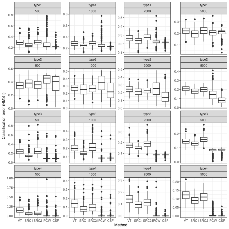
Figure 5: Classification error of different methods with RMST estimand. From left to right, top to bottom, the plots correspond to Scenarios 1-4, respectively. “VT” denotes the virtual twin method with random survival forests; “SRC1” denotes random survival forests using covariates $(X,W)$; “SRC2” denotes random survival forests using covariates $(X,W,XW)$. “IPCW” denotes a causal forest with Inverse Probability of Censoring Weighting; “CSF” denotes causal survival forest. Training size is (500, 1000, 2000 500), the number of covariates 15, the size of the test set 2000, and number of repetitions 250.

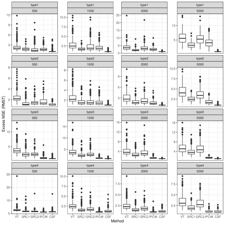
Figure 6: Excess MSE (defined as $\frac{1}{B}\sum_{b=1}^{B}MSE_{b}(method)/min(MSE_{b}(m)):m\in\{all\quad methods\}$) for different methods with RMST estimand in the four scenarios. From left to right, top to bottom, the plots correspond to Scenarios 1-4, respectively. “VT” denotes the virtual twin method with random survival forests; “SRC1” denotes random survival forests using covariates $(X,W)$; “SRC2” denotes random survival forests using covariates $(X,W,XW)$. “IPCW” denotes a causal forest with Inverse Probability of Censoring Weighting; “CSF” denotes causal survival forest. Training size is (500, 1000, 2000, 5000), the number of covariates 15, the size of the test set 2000, and the number of repetitions 250.

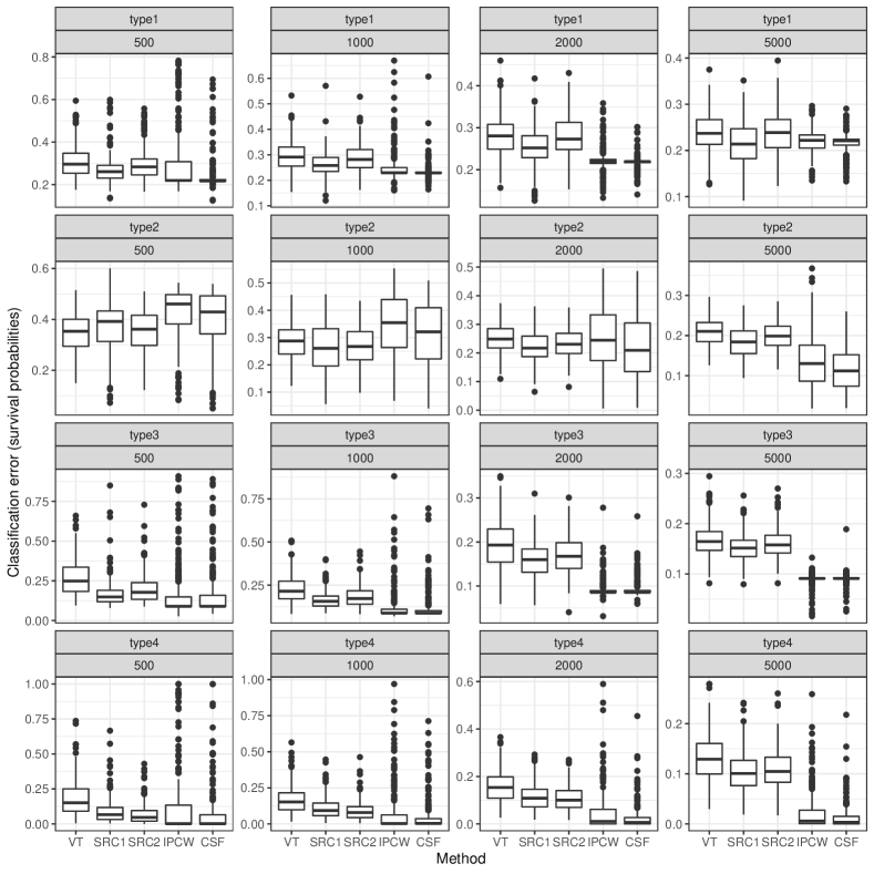
Figure 7: Classification error of different methods with survival probability estimand. From left to right, top to bottom, the plots correspond to Scenarios 1-4, respectively. “VT” denotes the virtual twin method with random survival forests; “SRC1” denotes random survival forests using covariates $(X,W)$; “SRC2” denotes random survival forests using covariates $(X,W,XW)$. “IPCW” denotes a causal forest with Inverse Probability of Censoring Weighting; “CSF” denotes causal survival forest. Training size is (500, 1000, 2000 500), the number of covariates 15, the size of the test set 2000, and number of repetitions 250.

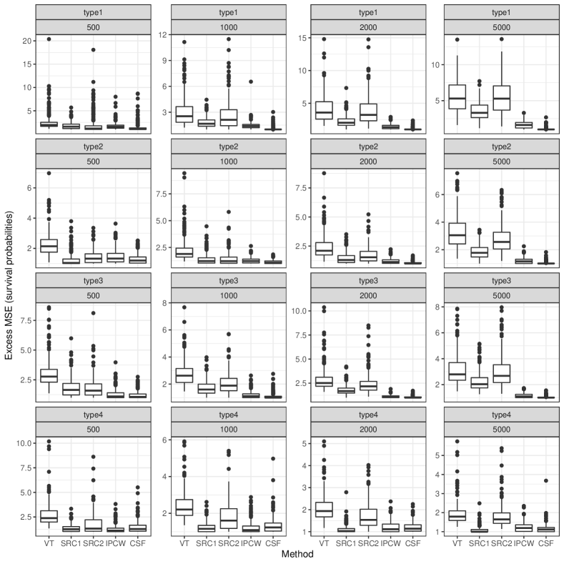
Figure 8: Excess MSE (defined as $\frac{1}{B}\sum_{b=1}^{B}MSE_{b}(method)/min(MSE_{b}(m)):m\in\{all\quad methods\}$) for different methods with survival probability estimand in the four scenarios. From left to right, top to bottom, the plots correspond to Scenarios 1-4, respectively. “VT” denotes the virtual twin method with random survival forests; “SRC1” denotes random survival forests using covariates $(X,W)$; “SRC2” denotes random survival forests using covariates $(X,W,XW)$. “IPCW” denotes a causal forest with Inverse Probability of Censoring Weighting; “CSF” denotes causal survival forest. Training size is (500, 1000, 2000, 5000), the number of covariates 15, the size of the test set 2000, and the number of repetitions 250.

Table 1 reports simulation results in terms of test set mean-squared error for $\tau(X_{i})$. Table 2 considers classification accuracy, i.e., $1-\frac{1}{n_{\text{test}}}\sum_{i=1}^{n_{\text{test}}}1\left\{\operatorname{sign}(\hat{\tau}(X_{i}))=\operatorname{sign}(\tau(X_{i}))\right\}$. These two tables report results with training set size $n=2000$, while Figures 5-8 in Section D in the Appendix show results across several values of $n$.

In almost all scenarios, the proposed causal survival forest achieves the best performance among all competing methods and, overall, the proposed causal survival forest is superior to ordinary random survival forests which do not target the causal parameter directly. The exception is for setting 4 where, when targeting RMST, IPCW performs best, and when targeting the survival probability, SRC1 performs best. IPCW generally outperforms the other baselines (except for setting 4 where SRC1 is best). Two aspects of our algorithm that may help explain this finding is that, first, both IPCW and CSF are designed to target treatment effects specifically, and so are able to focus on covariates interacting with $W$ rather than on the covariates which only appear in the main effect. Second, all of these simulation processes involve non-trivial right-censoring or confounding mechanism and, as emphasized throughout the paper, CSF was designed to robustly adjust for such censoring and confounding.

(a) Panel A: RMST

Setting	Metric	VT	SRC1	SRC2	IPCW	CSF
1	MSE	0.82	0.46	0.71	0.60	0.25
	Excess MSE	3.97	2.07	3.50	2.63	1.02
2	MSE	2.96	1.89	2.16	1.75	1.16
	Excess MSE	3.11	1.93	2.23	1.67	1.02
3	MSE	49.19	33.31	42.21	16.88	13.69
	Excess MSE	4.28	2.79	3.66	1.32	1.02
4	MSE	5.86	3.79	4.58	2.79	3.04
	Excess MSE	2.52	1.60	1.94	1.10	1.23

(b) Panel B: Survival probability

Setting	Metric	VT	SRC1	SRC2	IPCW	CSF
1	MSE	0.45	0.26	0.41	0.19	0.14
	Excess MSE	4.16	2.23	3.92	1.42	1.07
2	MSE	0.74	0.46	0.54	0.41	0.37
	Excess MSE	2.41	1.46	1.72	1.21	1.06
3	MSE	0.38	0.25	0.32	0.16	0.15
	Excess MSE	2.86	1.78	2.42	1.11	1.05
4	MSE	0.46	0.25	0.38	0.28	0.27
	Excess MSE	2.06	1.11	1.70	1.21	1.21

Table 1: Mean squared error (MSE) multiplied by 100 and excess MSE for four scenarios, defined as $\frac{1}{B}\sum_{b=1}^{B}\text{MSE}_{b}(\text{method})/\min\{\text{MSE}_{b}(m):m\in\{\text{all methods}\}\}$, respectively, for two estimands, RMST and survival probability. The simulation settings and methods under consideration are as described in Section 4. All forests were trained on $n=2000$ samples, and an independent test set with size $n_{\text{test}}=2000$ was used to evaluate error. Each simulation was repeated 250 times.

(a) Panel A: RMST

Setting	VT	SRC1	SRC2	IPCW	CSF
1	0.27	0.23	0.27	0.23	0.22
2	0.25	0.21	0.23	0.26	0.15
3	0.18	0.15	0.19	0.08	0.08
4	0.14	0.10	0.11	0.01	0.00

(b) Panel B: Survival probability

Setting	VT	SRC1	SRC2	IPCW	CSF
1	0.28	0.25	0.28	0.22	0.22
2	0.25	0.22	0.24	0.25	0.22
3	0.19	0.16	0.17	0.09	0.09
4	0.16	0.11	0.11	0.05	0.03

Table 2: Classification error for two estimands, RMST and survival probability, for four scenarios, defined as $1-\frac{1}{n_{\text{test}}}\sum_{i=1}^{n_{\text{test}}}1\left\{\operatorname{sign}(\hat{\tau}(X_{i}))=\operatorname{sign}(\tau(X_{i}))\right\}$ (for the last setting the classification error rate is evaluated on the subgroup of $X_{(1)}\geq 0.3$). The simulation settings and methods under consideration are as described in Section 4. All forests were trained on $n=2000$ samples, and an independent test set with size $n_{\text{test}}=2000$ was used to evaluate classification error. Each simulation was repeated 250 times.

Next, we consider the accuracy of the pointwise confidence intervals for causal survival forests proposed in Section 3.1. To do so, we evaluated the coverage of the proposed 95% confidence intervals at four deterministic points, namely $x_{1}=(0.2,\ldots,0.2)^{T}$, $x_{2}=(0.4,\ldots,0.4)^{T}$, $x_{3}=(0.6,\ldots,0.6)^{T}$ and $x_{4}=(0.8,\ldots,0.8)^{T}$. The true treatment effect was estimated by the Monte Carlo method with sample size 100000. The results, summarized in Table 3, are mostly promising, and suggests that in most of these examples the bias-variance trade off of causal survival forests puts us in a regime where discussions from Section 3.1 apply. However, at other points we observe poor coverage, especially at $x_{1}$ and $x_{4}$, which are near the corners of the feature space.

(a) Panel A: RMST

	Coverage				Length
Setting	$x_{1}$	$x_{2}$	$x_{3}$	$x_{4}$	$x_{1}$	$x_{2}$	$x_{3}$	$x_{4}$
1	0.84	0.69	0.88	0.95	0.09	0.08	0.15	0.18
2	0.75	0.93	0.92	0.82	0.32	0.25	0.21	0.23
3	0.82	0.96	0.89	0.72	0.96	0.81	0.82	0.95
4	0.37	0.68	0.96	0.88	0.36	0.31	0.32	0.39

(b) Panel B: Survival probability

	Coverage				Length
Setting	$x_{1}$	$x_{2}$	$x_{3}$	$x_{4}$	$x_{1}$	$x_{2}$	$x_{3}$	$x_{4}$
1	0.83	0.76	0.91	0.93	0.07	0.06	0.14	0.16
2	0.71	0.92	0.93	0.86	0.18	0.14	0.12	0.13
3	0.84	0.95	0.87	0.62	0.10	0.09	0.10	0.12
4	0.67	0.84	0.92	0.43	0.10	0.10	0.11	0.15

Table 3: Coverage (%) of the proposed 95% confidence intervals and average length at four deterministic points described in Section 4, with a training set size $n=2000$. $B=10000$ trees are used to fit confidence intervals. The numbers are aggregated over 1000 simulation replications.

Finally, we investigate the performance of the best linear projection estimator discussed in Section 3.2 which provides summaries of the CATE that are amenable to more robust inference. In Figure 2, given various choices of projection variables $A_{i}$ in (26), we consider both the doubly robust method of Semenova and Chernozhukov (2021) (DR) and a naive baseline that simply regresses the fitted $\hat{\tau}(X_{i})$ estimates against $A_{i}$ without a doubly robust correction (CATE). We find that the proposed BLP method performs well; in contrast, the naive direct regression can be biased (top row), and badly underestimates the sampling variability of these estimators, thus resulting in poor coverage (both rows).

Figure 2: First row: histogram of the estimated best linear projection (BLP) coefficient $\hat{\beta}_{1}$ in the regression $\hat{\tau}(x)=\hat{\beta}_{0}+\hat{\beta}_{1}X_{(1)}+\hat{\beta}_{2}X_{(2)}$, without (left) and with (right) a robustness correction to $\hat{\tau}(x)$, the estimated CATEs with CSF. Second row: histogram of the estimated coefficient $\beta_{0}$ (ATE) in the regression $\hat{\tau}(x)=\hat{\beta}_{0}$. The solid red line indicates the true population coefficient. Coverage is based on 95 % confidence intervals computed as $\hat{\beta}\pm z_{0.975}se(\hat{\beta})$, where $z$ is standard normal quantiles and $se(\hat{\beta})$ is derived via the $HC_{3}$ variance estimate (MacKinnon and White, 1985). Data is generated according to Setting 3 with $n=2000$ training samples and $p=15$ covariates. The number of repetitions is 500.

5 HIV data analysis

We demonstrate the proposed method by an application to the data from AIDS Clinical Trials Group Protocol 175 (ACTG175) (Hammer et al., 1996). The original dataset consists of 2139 HIV-infected subjects. The enrolled subjects were randomized to four treatment groups: zidovudine (ZDV) monotherapy, ZDV+didanosine (ddI), ZDV+zalcitabine, and ddI monotherapy. We focus on the subset of patients receiving the treatment ZDV+ddI or ddI monotherapy as considered in Lu et al. (2013). Treatment indicator $W=0$ denotes the treatment ddI with 561 subjects, and $W=1$ denotes the treatment ZDV+ddI with 522 subjects. Though ACTG175 is a randomized study, there seem to be some selection effects in the subsets used here. For example, for covariate race equals to 1, there are 138 receiving ZDV+ddI and 173 receiving ddI. A binomial test with null probability 0.5 gives p-value 0.05. For this reason, we analyze the study as an observational rather than randomized study.

Here we are interested in the causal effect between ZDV+ddI and ddI on survival time of HIV-infected patients. 12 selected baseline covariates were studied in Tsiatis et al. (2008); Zhang et al. (2008); Lu et al. (2013); Fan et al. (2017). There are 5 continuous covariates: age (year), weight (kg), Karnofsky score (scale of 0-100), CD4 count (cells/$\text{mm}^{3}$) at baseline, CD8 count (cells/$\text{mm}^{3}$) at baseline. There are 7 binary variables: gender (male = 1, female = 0), homosexual activity (yes = 1, no = 0), race (non-white = 1, white = 0), symptomatic status (symptomatic = 1, asymptomatic = 0), history of intravenous drug use (yes = 1, no = 0), hemophilia (yes = 1, no = 0), and antiretroviral history (experienced = 1, naive = 0). As the outcome considered here is the survival time, we also include CD4 count (cells/$\text{mm}^{3}$) at $20\pm 5$ weeks and CD8 count (cells/$\text{mm}^{3}$) at $20\pm 5$ weeks as covariates, in addition to the 12 covariates described above.

We applied the proposed causal survival forest to this dataset. We used the default tuning parameters, described in Section 4, with the exception of the number of trees which is set to $B=10000$ for computing confidence intervals. As mentioned in Section 2, Assumption 6 warrants some extra consideration. The high follow-up time in this study requires care in focusing on an appropriate estimand, namely a suitable $h$ for $T_{i}\land h$. This study includes a large amount of near end-time censored subjects observed up to almost 6 months after the last failure, which occurs at around 3 years. For this reason, we truncate the survival time right before 3 years, setting $h=1000$. This assures us that the estimated censoring probabilities $\hat{S}_{W_{i}}^{C}\left(U_{i}\land h\,\big{|}\,X_{i}\right)$ all lie in a reasonable range and suggest that we are in a regime where this identifying assumption holds. Figure 3 shows a histogram depicting the issue. In the raw data, the observations with the largest values of $T_{i}$ are all censored, and so moments of $T_{i}$ are not identified. However, given a focus on restricted survival time with a judicious choice of $h$, we get to re-code all (censored or uncensored) observations with $U_{i}>h$ as uncensored observations with $T_{i}=h$, thus eliminating the positivity problem.

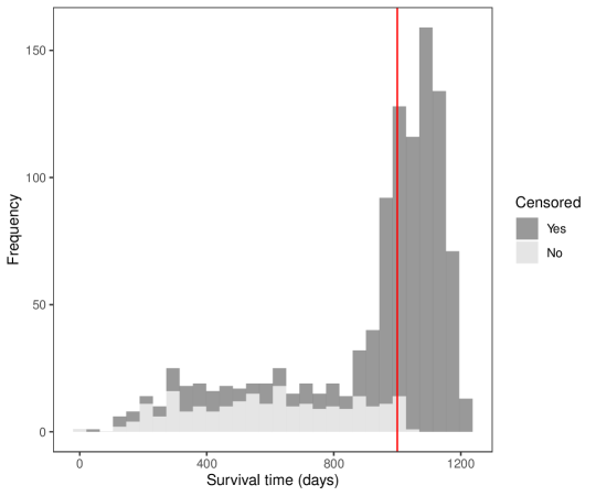
Figure 3: Histogram of survival time for censored/non-censored subjects. The solid red line is the suggested truncation time $h=1000$. The data is from the AIDS Clinical Trials Group Protocol 175 (ACTG175) (Hammer et al., 1996) with control set to the didanosine treatment with 561 subjects and the treatment group to zidovudine+didanosine with 522 subjects.

Following Lu et al. (2013) and Fan et al. (2017) we consider what role age serves in treatment efficacy. Figure 4 shows the estimated CATEs against age with all other covariates set to their median value, and as the plot suggests, age appears to have a positive effect, with older patients benefiting more from the treatment ZDV+ddI. Table 4 shows point estimates and standard errors from a random sample of patients. We also consider the best linear projection proposed in Section 3.2, in particular, we regress the obtained doubly robust scores on all covariates, and age only. The results in Table 5 suggest that we should exercise caution in interpreting heterogeneity in $\hat{\tau}(\cdot)$, as none of the coefficients in the considered projections are significantly from zero.

CATE	se(CATE)	Hemophilia	Gender	Homosexual activity	Antiretroviral history
-7.90	10.45	No	Male	Yes	Experienced
-6.90	13.89	No	Male	Yes	Naive
-4.38	17.06	No	Male	Yes	Naive
0.43	17.28	No	Male	No	Naive
7.26	19.17	No	Male	No	Naive
8.20	11.45	No	Male	Yes	Naive
12.80	13.82	No	Female	Yes	Naive
13.42	14.16	No	Male	Yes	Naive
14.95	14.13	No	Male	Yes	Naive
19.99	43.53	Yes	Male	No	Experienced

Table 4: CATE estimates and standard errors from a random sample of 10 individuals as well as patient characteristics corresponding to the four covariates with the highest split frequency obtained from fitting a causal survival forest with default options (survival time threshold at $1000$ days) on data from AIDS Clinical Trials Group Protocol 175. The data is from Hammer et al. (1996) with control set to the didanosine treatment with 561 subjects and the treatment group to zidovudine+didanosine with 522 subjects.

Figure 4: Estimated CATEs (survival time in days) versus age (in years) and 95 % confidence bars (dash lines), with all other covariates set to their median value. CATEs are estimated using a causal survival forest with default options (the number of trees is set to 10 000 for confidence intervals) and the survival time threshold at $1000$ days. The data is from AIDS Clinical Trials Group Protocol 175 (ACTG175) (Hammer et al., 1996) with control set to the didanosine treatment with 561 subjects and the treatment group to zidovudine+didanosine with 522 subjects. 14 covariates are included in the analysis, 5 continuous: age (year), weight (kg), Karnofsky score (scale of 0-100), CD4 count (cells/$\text{mm}^{3}$) at baseline, and at $20\pm 5$ weeks, CD8 count (cells/$\text{mm}^{3}$) at baseline, and at $20\pm 5$ weeks, and 7 binary: gender (male = 1, female = 0), homosexual activity (yes = 1, no = 0), race (non-white = 1, white = 0), symptomatic status (symptomatic = 1, asymptomatic = 0), history of intravenous drug use (yes = 1, no = 0), hemophilia (yes = 1, no = 0), and antiretroviral history (experienced = 1, naive = 0).

	All covariates	Age only
Constant	$-151.65\;(240.10)$	$-25.85\;(48.49)$
Age	$1.26\;(1.46)$	$1.01\;(1.35)$
Weight	$-1.99\;(1.02)$
Karnofsky score	$2.75\;(2.13)$
CD4 count	$-0.06\;(0.13)$
CD8 count	$0.05\;(0.05)$
Gender	$44.15\;(41.90)$
Homosexual activity	$-33.08\;(34.47)$
Race	$31.61\;(25.61)$
Symptomatic status	$-10.08\;(35.40)$
Intravenous drug use	$48.36\;(31.94)$
Hemophilia	$-63.46\;(44.97)$
Antiretroviral history	$-7.57\;(24.11)$
CD4 count 20+/-5 weeks	$-0.03\;(0.11)$
CD8 count 20+/-5 weeks	$-0.04\;(0.04)$
$HC_{3}$ (MacKinnon and White, 1985) standard errors in parentheses.

Table 5: Best linear projection $\hat{\tau}_{DR}(x)=\hat{\beta}_{0}+A\hat{\beta}$ on doubly robust estimates obtained from fitting a causal survival forest with default options (survival time threshold at $1000$ days) on data from AIDS Clinical Trials Group Protocol 175. The data is from Hammer et al. (1996) with control set to the didanosine treatment with 561 subjects and the treatment group to zidovudine+didanosine with 522 subjects. 14 covariates are included in the analysis, 5 continuous: age (year), weight (kg), Karnofsky score (scale of 0-100), CD4 count (cells/$\text{mm}^{3}$) at baseline, and at $20\pm 5$ weeks, CD8 count (cells/$\text{mm}^{3}$) at baseline, and at $20\pm 5$ weeks, and 7 binary: gender (male = 1, female = 0), homosexual activity (yes = 1, no = 0), race (non-white = 1, white = 0), symptomatic status (symptomatic = 1, asymptomatic = 0), history of intravenous drug use (yes = 1, no = 0), hemophilia (yes = 1, no = 0), and antiretroviral history (experienced = 1, naive = 0).

Appendix

Appendix A Proof of Proposition 1

To simplify the notation, we write $T\land h$ as $\tilde{T}$ and $U\land h$ as $\tilde{U}$ in this section. We first start with a proof in the context of estimating $\mu=\mu(x)=\mathbb{E}\left[y(T)\right]$ by the estimating equation (9), which might also be of independent interest. Namely, we show that

$$\hat{\mu}-\tilde{\mu}=o_{p}(\max(c_{n}^{2},c_{n}d_{n})),$$ (28)

where $\tilde{\mu}$ is an oracle estimator for $\mu$.

Proof of (28).

At a high level, cross-fitting uses cross-fold estimation to avoid bias due to overfitting. Recall that the cross-fitting first splits the data (at random) into two halves $I_{1}$ and $I_{2}$, and then uses an estimator

$$\hat{\mu}=\frac{n_{1}}{n}\hat{\mu}^{I_{1}}+\frac{n_{2}}{n}\hat{\mu}^{I_{2}},$$

where $n_{1}=|I_{1}|$, $n_{2}=|I_{2}|$, and $\hat{\mu}^{I_{1}},\hat{\mu}^{I_{2}}$ are estimated using nuisances estimated from samples $I_{2},I_{1}$, respectively. We essentially need to show that

$$\hat{\mu}^{I_{1}}-\tilde{\mu}^{I_{1}}=o_{p}(\max(c_{n}^{2},c_{n}d_{n})),$$

where $\tilde{\mu}^{I_{1}}$ is the oracle estimator obtained by solving

$$\frac{1}{n_{1}}\sum_{i:i\in I_{1}}\frac{\Delta^{h}_{i}(y(U_{i})-\mu)}{S^{C}(\tilde{U}_{i}|X_{i})}+\frac{(1-\Delta^{h}_{i})}{S^{C}(\tilde{U}_{i}|X_{i})}\mathbb{E}\left[y(T_{i})-\mu\,\big{|}\,X_{i},\,\tilde{T}_{i}>\tilde{U}_{i}\right]-\int_{0}^{\tilde{U}_{i}}\frac{\lambda^{C}(s|X_{i})}{S^{C}(s|X_{i})}\mathbb{E}\left[y(T_{i})-\mu\,\big{|}\,X_{i},\,\tilde{T}_{i}>s\right]ds=0.$$

Note that we have the following decomposition of $\hat{\mu}^{I_{1}}-\tilde{\mu}^{I_{1}}$

$$\hat{\mu}^{I_{1}}-\tilde{\mu}^{I_{1}}$$

$$= \frac{1}{n_{1}}\left[\sum_{i:i\in I_{1}}\Delta^{h}_{i}\frac{y(U_{i})}{\hat{S}^{C}(\tilde{U}_{i}|X_{i})}+(1-\Delta^{h}_{i})\frac{\hat{Q}(\tilde{U}_{i}|X_{i})}{{\hat{S}^{C}(\tilde{U}_{i}|X_{i})}}-\int_{0}^{\tilde{U}_{i}}\frac{\hat{\lambda}^{C}(s|X_{i})}{\hat{S}^{C}(s|X_{i})}\hat{Q}(s|X_{i})ds\right]$$

$$-\frac{1}{n_{1}}\left[\sum_{i:i\in I_{1}}\Delta^{h}_{i}\frac{y(U_{i})}{S^{C}(\tilde{U}_{i}|X_{i})}+(1-\Delta^{h}_{i})\frac{Q(\tilde{U}_{i}|X_{i})}{{S^{C}(\tilde{U}_{i}|X_{i})}}-\int_{0}^{\tilde{U}_{i}}\frac{\lambda^{C}(s|X_{i})}{S^{C}(s|X_{i})}Q(s|X_{i})ds\right]$$

$$= \frac{1}{n_{1}}\Bigg{[}\sum_{i:i\in I_{1}}\frac{(1-\Delta^{h}_{i})}{S^{C}(\tilde{U}_{i}|X_{i})}(\hat{Q}(\tilde{U}_{i}|X_{i})-Q(\tilde{U}_{i}|X_{i}))-\int_{0}^{\tilde{U}_{i}}\frac{\lambda^{C}(s|X_{i})}{S^{C}(s|X_{i})}(\hat{Q}(s|X_{i})-Q(s|X_{i}))ds$$

$$+(1-\Delta^{h}_{i})(\frac{1}{\hat{S}^{C}(\tilde{U}_{i}|X_{i})}-\frac{1}{S^{C}(\tilde{U}_{i}|X_{i})})(\hat{Q}(\tilde{U}_{i}|X_{i})-Q(\tilde{U}_{i}|X_{i}))$$

$$-\int_{0}^{\tilde{U}_{i}}(\frac{\hat{\lambda}^{C}(s|X_{i})}{\hat{S}^{C}(s|X_{i})}-\frac{\lambda^{C}(s|X_{i})}{S^{C}(s|X_{i})})(\hat{Q}(s|X_{i})-Q(s|X_{i}))ds$$

$$+(1-\Delta^{h}_{i})(\frac{1}{\hat{S}^{C}(\tilde{U}_{i}|X_{i})}-\frac{1}{S^{C}(\tilde{U}_{i}|X_{i})})Q(\tilde{U}_{i}|X_{i})+\Delta^{h}_{i}(\frac{1}{\hat{S}^{C}(\tilde{U}_{i}|X_{i})}-\frac{1}{S^{C}(\tilde{U}_{i}|X_{i})})y(U_{i})$$

$$-\int_{0}^{\tilde{U}_{i}}(\frac{\hat{\lambda}^{C}(s|X_{i})}{\hat{S}^{C}(s|X_{i})}-\frac{\lambda^{C}(s|X_{i})}{S^{C}(s|X_{i})})Q(s|X_{i})ds\Bigg{]},$$ (29)

where we denote $\widehat{\mathbb{E}}\left[y(T_{i})|\tilde{T}_{i}>\tilde{U}_{i},\,\,X_{i}\right]$ by $\hat{Q}(\tilde{U}_{i}|X_{i})$, and $\mathbb{E}\left[y(T_{i})|\tilde{T}_{i}>\tilde{U}_{i},\,\,X_{i}\right]$ by $Q(\tilde{U}_{i}|X_{i})$. At a high level, this decomposition separates $\hat{\mu}^{I_{1}}-\tilde{\mu}^{I_{1}}$ to four terms: two mean zero terms and two product terms.

Note that by the double robustness of equation (9) shown in Tsiatis [2007, Chapter 10.4],

$$\mathbb{E}\left[\frac{(1-\Delta^{h}_{i})}{S^{C}(\tilde{U}_{i}|X_{i})}(\hat{Q}(\tilde{U}_{i}|X_{i})-Q(\tilde{U}_{i}|X_{i}))-\int_{0}^{\tilde{U}_{i}}\frac{\lambda^{C}(s|X_{i})}{S^{C}(s|X_{i})}(\hat{Q}(s|X_{i})-Q(s|X_{i}))ds\right]=0.$$

Thanks to our cross-fitting construction, the nuisance components can effectively be treated as deterministic. Thus, after conditioning on $I_{2}$, the summands used to build the following term become mean-zero and independent:

$$\mathbb{E}\left[\left(\frac{1}{n_{1}}\sum_{i:i\in I_{1}}\frac{(1-\Delta^{h}_{i})}{S^{C}(\tilde{U}_{i}|X_{i})}(\hat{Q}(\tilde{U}_{i}|X_{i})-Q(\tilde{U}_{i}|X_{i}))-\int_{0}^{\tilde{U}_{i}}\frac{\lambda^{C}(s|X_{i})}{S^{C}(s|X_{i})}(\hat{Q}(s|X_{i})-Q(s|X_{i}))ds\right)^{2}\right]$$

$$= \mathbb{E}\left[\mathbb{E}\left[\left(\frac{1}{n_{1}}\sum_{i:i\in I_{1}}\frac{(1-\Delta^{h}_{i})}{S^{C}(\tilde{U}_{i}|X_{i})}(\hat{Q}(\tilde{U}_{i}|X_{i})-Q(\tilde{U}_{i}|X_{i}))-\int_{0}^{\tilde{U}_{i}}\frac{\lambda^{C}(s|X_{i})}{S^{C}(s|X_{i})}(\hat{Q}(s|X_{i})-Q(s|X_{i}))ds\right)^{2}\Bigg{|}I_{2}\right]\right]$$

$$= \mathbb{E}\left[\operatorname{Var}\left[\left(\frac{1}{n_{1}}\sum_{i:i\in I_{1}}\frac{(1-\Delta^{h}_{i})}{S^{C}(\tilde{U}_{i}|X_{i})}(\hat{Q}(\tilde{U}_{i}|X_{i})-Q(\tilde{U}_{i}|X_{i}))-\int_{0}^{\tilde{U}_{i}}\frac{\lambda^{C}(s|X_{i})}{S^{C}(s|X_{i})}(\hat{Q}(s|X_{i})-Q(s|X_{i}))ds\right)\Bigg{|}I_{2}\right]\right]$$

$$= \frac{1}{n_{1}}\mathbb{E}\left[\operatorname{Var}\left[\left(\frac{(1-\Delta^{h}_{i})}{S^{C}(\tilde{U}_{i}|X_{i})}(\hat{Q}(\tilde{U}_{i}|X_{i})-Q(\tilde{U}_{i}|X_{i}))-\int_{0}^{\tilde{U}_{i}}\frac{\lambda^{C}(s|X_{i})}{S^{C}(s|X_{i})}(\hat{Q}(s|X_{i})-Q(s|X_{i}))ds\right)\Bigg{|}I_{2}\right]\right]$$

$$\leq \frac{O_{p}(1)}{n_{1}}\sup_{x\in\mathcal{X},s\leq h}|\hat{Q}(s|x)-Q(s|x)|^{2}=\frac{o_{p}(1)}{n}.$$ (30)

The same logic applies to the term

$$(1-\Delta^{h}_{i})(\frac{1}{\hat{S}^{C}(\tilde{U}_{i}|X_{i})}-\frac{1}{S^{C}(\tilde{U}_{i}|X_{i})})Q(\tilde{U}_{i}|X_{i})+\Delta^{h}_{i}(\frac{1}{\hat{S}^{C}(\tilde{U}_{i}|X_{i})}-\frac{1}{S^{C}(\tilde{U}_{i}|X_{i})})y(U_{i})$$

$$-\int_{0}^{\tilde{U}_{i}}(\frac{\hat{\lambda}^{C}(s|X_{i})}{\hat{S}^{C}(s|X_{i})}-\frac{\lambda^{C}(s|X_{i})}{S^{C}(s|X_{i})})Q(s|X_{i})ds,$$

as

$$\mathbb{E}\bigg{(}(1-\Delta^{h}_{i})(\frac{1}{\hat{S}^{C}(\tilde{U}_{i}|X_{i})}-\frac{1}{S^{C}(\tilde{U}_{i}|X_{i})})Q(\tilde{U}_{i}|X_{i})+\Delta^{h}_{i}(\frac{1}{\hat{S}^{C}(\tilde{U}_{i}|X_{i})}-\frac{1}{S^{C}(\tilde{U}_{i}|X_{i})})y(U_{i})$$

$$-\int_{0}^{\tilde{U}_{i}}(\frac{\hat{\lambda}^{C}(s|X_{i})}{\hat{S}^{C}(s|X_{i})}-\frac{\lambda^{C}(s|X_{i})}{S^{C}(s|X_{i})})Q(s|X_{i})ds\bigg{)}=0,$$

so we have that

$$\mathbb{E}\bigg{(}\frac{1}{n_{1}}\sum_{i:i\in I_{1}}(1-\Delta^{h}_{i})(\frac{1}{\hat{S}^{C}(\tilde{U}_{i}|X_{i})}-\frac{1}{S^{C}(\tilde{U}_{i}|X_{i})})Q(\tilde{U}_{i}|X_{i})+\Delta^{h}_{i}(\frac{1}{\hat{S}^{C}(\tilde{U}_{i}|X_{i})}-\frac{1}{S^{C}(\tilde{U}_{i}|X_{i})})y(U_{i})$$

$$-\int_{0}^{\tilde{U}_{i}}(\frac{\hat{\lambda}^{C}(s|X_{i})}{\hat{S}^{C}(s|X_{i})}-\frac{\lambda^{C}(s|X_{i})}{S^{C}(s|X_{i})})Q(s|X_{i})ds\bigg{)}\leq\frac{o_{p}(1)}{n}.$$ (31)

In addition, by Cauchy-Schwarz inequality,

$$\frac{1}{n_{1}}\sum_{i:i\in I_{1}}\bigg{(}(1-\Delta^{h}_{i})(\frac{1}{\hat{S}^{C}(\tilde{U}_{i}|X_{i})}-\frac{1}{S^{C}(\tilde{U}_{i}|X_{i})})(\hat{Q}(\tilde{U}_{i}|X_{i})-Q(\tilde{U}_{i}|X_{i}))$$

$$-\int_{0}^{\tilde{U}_{i}}(\frac{\hat{\lambda}^{C}(s|X_{i})}{\hat{S}^{C}(s|X_{i})}-\frac{\lambda^{C}(s|X_{i})}{S^{C}(s|X_{i})})(\hat{Q}(s|X_{i})-Q(s|X_{i}))ds\bigg{)}$$

$$\leq \sqrt{\frac{1}{n_{1}}\sum_{i:i\in I_{1}}(1-\Delta^{h}_{i})(\frac{1}{\hat{S}^{C}(\tilde{U}_{i}|X_{i})}-\frac{1}{S^{C}(\tilde{U}_{i}|X_{i})})^{2}}\times\sqrt{\frac{1}{n_{1}}\sum_{i:i\in I_{1}}(1-\Delta^{h}_{i})(\hat{Q}(\tilde{U}_{i}|X_{i})-Q(\tilde{U}_{i}|X_{i}))^{2}}$$

$$+\int_{0}^{\tilde{U}_{i}}\sqrt{\frac{1}{n_{1}}\sum_{i:i\in I_{1}}(\frac{\hat{\lambda}^{C}(s|X_{i})}{\hat{S}^{C}(s|X_{i})}-\frac{\lambda^{C}(s|X_{i})}{S^{C}(s|X_{i})})^{2}}\times\sqrt{\frac{1}{n_{1}}\sum_{i:i\in I_{1}}(\hat{Q}(s|X_{i})-Q(s|X_{i}))^{2}}ds$$

$$= o_{p}(\max(c_{n}^{2},c_{n}d_{n})).$$ (32)

Therefore, combining equations (30), (31), and (32), we have that $\hat{\mu}-\tilde{\mu}=o_{p}(\max(c_{n}^{2},c_{n}d_{n}))$. ∎

Now, we turn to estimating $\tau=\tau(x)=\mathbb{E}\left[y(T(1))-y(T(0))\right]$.

Proof of Proposition 1.

Using the same notation as the proof of equation (28) and consider an estimator

$$\hat{\tau}=\frac{n_{1}}{n}\hat{\tau}^{I_{1}}+\frac{n_{2}}{n}\hat{\tau}^{I_{2}},$$

where $n_{1}=|I_{1}|$, $n_{2}=|I_{2}|$, and $\hat{\tau}^{I_{1}},\hat{\tau}^{I_{2}}$ are estimated using nuisances estimated from samples $I_{2},I_{1}$, respectively. Note that

$$\hat{\tau}^{I_{1}}-\tilde{\tau}^{I_{1}}$$

$$= \bigg{(}\frac{1}{n_{1}}\sum_{i:i\in I_{1}}(W_{i}-\hat{e}(X_{i}))^{2}\bigg{)}^{-1}\frac{1}{n_{1}}\sum_{i:i\in I_{1}}\bigg{(}\frac{\hat{\Upsilon}_{i}}{\hat{S}^{C}_{W_{i}}(\tilde{U}_{i}|X_{i})}-\int_{0}^{\tilde{U}_{i}}\frac{\hat{\lambda}_{W_{i}}^{C}(s|X_{i})}{\hat{S}^{C}_{W_{i}}(s|X_{i})}(W_{i}-\hat{e}(X_{i}))[\hat{Q}_{W_{i}}(s|X_{i})-\hat{m}(X_{i})]ds\bigg{)}$$

$$-\bigg{(}\frac{1}{n_{1}}\sum_{i:i\in I_{1}}(W_{i}-e(X_{i}))^{2}\bigg{)}^{-1}\frac{1}{n_{1}}\sum_{i:i\in I_{1}}\bigg{(}\frac{\Upsilon_{i}}{S^{C}_{W_{i}}(\tilde{U}_{i}|X_{i})}-\int_{0}^{\tilde{U}_{i}}\frac{\lambda_{W_{i}}^{C}(s|X_{i})}{S^{C}_{W_{i}}(s|X_{i})}(W_{i}-e(X_{i}))[Q_{W_{i}}(s|X_{i})-m(X_{i})]ds\bigg{)},$$

where $\tilde{\tau}^{I_{1}}$ is the oracle estimator,

$$\Upsilon_{i} =\begin{cases}\{W_{i}-e(X_{i})\}\{y(U_{i})-m(X_{i})\}&\text{if}\quad\Delta^{h}_{i}=1,\\ \{W_{i}-e(X_{i})\}\{Q_{W_{i}}(\tilde{U}_{i}|X_{i})-m(X_{i})\}&\text{o.w.}\end{cases}$$

and

$$\hat{\Upsilon}_{i} =\begin{cases}\{W_{i}-\hat{e}(X_{i})\}\{y(U_{i})-\hat{m}(X_{i})\}&\text{if}\quad\Delta^{h}_{i}=1,\\ \{W_{i}-\hat{e}(X_{i})\}\{\hat{Q}_{W_{i}}(\tilde{U}_{i}|X_{i})-\hat{m}(X_{i})\}&\text{o.w.}\end{cases}$$

Denote $\hat{\tau}^{I_{1}}-\tilde{\tau}^{I_{1}}$ by

$$\frac{K_{1}}{J_{1}}-\frac{K_{2}}{J_{2}}.$$

Thus, we have

$$\frac{K_{1}}{J_{1}}-\frac{K_{2}}{J_{2}}=\frac{K_{1}+K_{2}-K_{2}}{J_{1}}-\frac{K_{2}}{J_{2}}$$

$$= \frac{K_{1}-K_{2}}{J_{1}}+K_{2}(\frac{1}{J_{1}}-\frac{1}{J_{2}})=\frac{K_{1}-K_{2}}{J_{1}}+\frac{K_{2}}{J_{1}J_{2}}(J_{2}-J_{1}).$$ (33)

We essentially need to bound $K_{1}-K_{2}$, and we have the following decomposition,

$$K_{1}-K_{2}= \frac{1}{n_{1}}\bigg{[}\sum_{i:i\in I_{1}}\Delta^{h}_{i}\frac{\{W_{i}-\hat{e}(X_{i})\}\{y(U_{i})-\hat{m}(X_{i})\}}{\hat{S}^{C}_{W_{i}}(\tilde{U}_{i}|X_{i})}+(1-\Delta^{h}_{i})\frac{\{W_{i}-\hat{e}(X_{i})\}\{\hat{Q}_{W_{i}}(\tilde{U}_{i}|X_{i})-\hat{m}(X_{i})\}}{{\hat{S}^{C}_{W_{i}}(\tilde{U}_{i}|X_{i})}}$$

$$-\int_{0}^{\tilde{U}_{i}}\frac{\hat{\lambda}_{W_{i}}^{C}(s|X_{i})}{\hat{S}^{C}_{W_{i}}(s|X_{i})}(W_{i}-\hat{e}(X_{i}))[\hat{Q}_{W_{i}}(s|X_{i})-\hat{m}(X_{i})]ds$$

$$-\Delta^{h}_{i}\frac{\{W_{i}-e(X_{i})\}\{y(U_{i})-m(X_{i})\}}{S^{C}_{W_{i}}(\tilde{U}_{i}|X_{i})}-(1-\Delta^{h}_{i})\frac{\{W_{i}-e(X_{i})\}\{Q_{W_{i}}(\tilde{U}_{i}|X_{i})-m(X_{i})\}}{{S^{C}_{W_{i}}(\tilde{U}_{i}|X_{i})}}$$

$$+\int_{0}^{\tilde{U}_{i}}\frac{\lambda_{W_{i}}^{C}(s|X_{i})}{S^{C}_{W_{i}}(s|X_{i})}(W_{i}-e(X_{i}))[Q_{W_{i}}(s|X_{i})-m(X_{i})]ds\bigg{]}$$

$$= \frac{1}{n_{1}}\bigg{[}\sum_{i:i\in I_{1}}\Delta^{h}_{i}\frac{\{W_{i}-\hat{e}(X_{i})\}\{y(U_{i})-\hat{m}(X_{i})\}}{\hat{S}^{C}_{W_{i}}(\tilde{U}_{i}|X_{i})}+(1-\Delta^{h}_{i})\frac{\{W_{i}-\hat{e}(X_{i})\}\{\hat{Q}_{W_{i}}(\tilde{U}_{i}|X_{i})-\hat{m}(X_{i})\}}{{\hat{S}^{C}_{W_{i}}(\tilde{U}_{i}|X_{i})}}$$

$$-\int_{0}^{\tilde{U}_{i}}\frac{\hat{\lambda}_{W_{i}}^{C}(s|X_{i})}{\hat{S}^{C}_{W_{i}}(s|X_{i})}(W_{i}-\hat{e}(X_{i}))[\hat{Q}_{W_{i}}(s|X_{i})-\hat{m}(X_{i})]ds$$

$$-\Delta^{h}_{i}\frac{\{W_{i}-\hat{e}(X_{i})\}\{y(U_{i})-\hat{m}(X_{i})\}}{S^{C}_{W_{i}}(\tilde{U}_{i}|X_{i})}-(1-\Delta^{h}_{i})\frac{\{W_{i}-\hat{e}(X_{i})\}\{Q_{W_{i}}(\tilde{U}_{i}|X_{i})-\hat{m}(X_{i})\}}{{S^{C}_{W_{i}}(\tilde{U}_{i}|X_{i})}}$$

$$+\int_{0}^{\tilde{U}_{i}}\frac{\lambda_{W_{i}}^{C}(s|X_{i})}{S^{C}_{W_{i}}(s|X_{i})}(W_{i}-\hat{e}(X_{i}))[Q_{W_{i}}(s|X_{i})-\hat{m}(X_{i})]ds$$

$$+\Delta^{h}_{i}\frac{\{W_{i}-\hat{e}(X_{i})\}\{y(U_{i})-\hat{m}(X_{i})\}}{S^{C}_{W_{i}}(\tilde{U}_{i}|X_{i})}+(1-\Delta^{h}_{i})\frac{\{W_{i}-\hat{e}(X_{i})\}\{Q_{W_{i}}(\tilde{U}_{i}|X_{i})-\hat{m}(X_{i})\}}{{S^{C}_{W_{i}}(\tilde{U}_{i}|X_{i})}}$$

$$-\int_{0}^{\tilde{U}_{i}}\frac{\lambda_{W_{i}}^{C}(s|X_{i})}{S^{C}_{W_{i}}(s|X_{i})}(W_{i}-\hat{e}(X_{i}))[Q_{W_{i}}(s|X_{i})-\hat{m}(X_{i})]ds$$

$$-\Delta^{h}_{i}\frac{\{W_{i}-e(X_{i})\}\{y(U_{i})-m(X_{i})\}}{S^{C}_{W_{i}}(\tilde{U}_{i}|X_{i})}-(1-\Delta^{h}_{i})\frac{\{W_{i}-e(X_{i})\}\{Q_{W_{i}}(\tilde{U}_{i}|X_{i})-m(X_{i})\}}{{S^{C}_{W_{i}}(\tilde{U}_{i}|X_{i})}}$$

$$+\int_{0}^{\tilde{U}_{i}}\frac{\lambda_{W_{i}}^{C}(s|X_{i})}{S^{C}_{W_{i}}(s|X_{i})}(W_{i}-e(X_{i}))[Q_{W_{i}}(s|X_{i})-m(X_{i})]ds\bigg{]}.$$

At a high level, this decomposition separates $K_{1}-K_{2}$ into two terms: the first term takes $\hat{m}$ and $\hat{e}$ as given, and follow the construction in the survival-related nuisance components (A) to bound errors caused by using $\hat{\lambda}^{C}_{w},\,\hat{S}^{C}_{w},\,\hat{Q}_{w}$ instead of ${\lambda}^{C}_{w},\,{S}^{C}_{w},\,{Q}_{w}$; the second term bounds errors caused by using $\hat{m}$ and $\hat{e}$ instead of ${m}$ and ${e}$.

For the term

$$\Delta^{h}_{i}\frac{\{W_{i}-\hat{e}(X_{i})\}\{y(U_{i})-\hat{m}(X_{i})\}}{\hat{S}^{C}_{W_{i}}(\tilde{U}_{i}|X_{i})}+(1-\Delta^{h}_{i})\frac{\{W_{i}-\hat{e}(X_{i})\}\{\hat{Q}_{W_{i}}(\tilde{U}_{i}|X_{i})-\hat{m}(X_{i})\}}{{\hat{S}^{C}_{W_{i}}(\tilde{U}_{i}|X_{i})}}$$

$$-\int_{0}^{\tilde{U}_{i}}\frac{\hat{\lambda}_{W_{i}}^{C}(s|X_{i})}{\hat{S}^{C}_{W_{i}}(s|X_{i})}(W_{i}-\hat{e}(X_{i}))[\hat{Q}_{W_{i}}(s|X_{i})-\hat{m}(X_{i})]ds$$

$$-\Delta^{h}_{i}\frac{\{W_{i}-\hat{e}(X_{i})\}\{y(U_{i})-\hat{m}(X_{i})\}}{S^{C}_{W_{i}}(U_{i}|X_{i})}-(1-\Delta^{h}_{i})\frac{\{W_{i}-\hat{e}(X_{i})\}\{Q_{W_{i}}(\tilde{U}_{i}|X_{i})-\hat{m}(X_{i})\}}{{S^{C}_{W_{i}}(\tilde{U}_{i}|X_{i})}}$$

$$+\int_{0}^{\tilde{U}_{i}}\frac{\lambda_{W_{i}}^{C}(s|X_{i})}{S^{C}_{W_{i}}(s|X_{i})}(W_{i}-\hat{e}(X_{i}))[Q_{W_{i}}(s|X_{i})-\hat{m}(X_{i})]ds\equiv(I),$$

the proof follows from the same decomposition of equation (A) with $\tilde{U}_{i}$ replaced by $\{W_{i}-\hat{e}(X_{i})\}\{\tilde{U}_{i}-\hat{m}(X_{i})\}$ and $\hat{Q}(\tilde{U}_{i}|X_{i})$ replaced by $\{W_{i}-\hat{e}(X_{i})\}\{\hat{Q}_{W_{i}}(\tilde{U}_{i}|X_{i})-\hat{m}(X_{i})\}$. So we have that

$$(I)=o_{p}(c_{n}^{2}+c_{n}d_{n}).$$ (34)

For the term

$$\Delta^{h}_{i}\frac{\{W_{i}-\hat{e}(X_{i})\}\{y(U_{i})-\hat{m}(X_{i})\}}{S^{C}_{W_{i}}(\tilde{U}_{i}|X_{i})}+(1-\Delta^{h}_{i})\frac{\{W_{i}-\hat{e}(X_{i})\}\{Q_{W_{i}}(\tilde{U}_{i}|X_{i})-\hat{m}(X_{i})\}}{{S^{C}_{W_{i}}(\tilde{U}_{i}|X_{i})}}$$

$$-\int_{0}^{\tilde{U}_{i}}\frac{\lambda_{W_{i}}^{C}(s|X_{i})}{S^{C}_{W_{i}}(s|X_{i})}(W_{i}-\hat{e}(X_{i}))[Q_{W_{i}}(s|X_{i})-\hat{m}(X_{i})]ds$$

$$-\Delta^{h}_{i}\frac{\{W_{i}-e(X_{i})\}\{y(U_{i})-m(X_{i})\}}{S^{C}_{W_{i}}(\tilde{U}_{i}|X_{i})}-(1-\Delta^{h}_{i})\frac{\{W_{i}-e(X_{i})\}\{Q_{W_{i}}(\tilde{U}_{i}|X_{i})-m(X_{i})\}}{{S^{C}_{W_{i}}(\tilde{U}_{i}|X_{i})}}$$

$$+\int_{0}^{\tilde{U}_{i}}\frac{\lambda_{W_{i}}^{C}(s|X_{i})}{S^{C}_{W_{i}}(s|X_{i})}(W_{i}-e(X_{i}))[Q_{W_{i}}(s|X_{i})-m(X_{i})]ds\equiv(II),$$

we have the following decomposition of $(II)$,

$$\frac{\Delta^{h}_{i}}{S^{C}_{W_{i}}(\tilde{U}_{i}|X_{i})}[(e(X_{i})-\hat{e}(X_{i}))(m(X_{i})-\hat{m}(X_{i}))+(e(X_{i})-\hat{e}(X_{i}))(y(U_{i})-m(X_{i}))+(W_{i}-e(X_{i}))(m(X_{i})-\hat{m}(X_{i}))]$$

$$+\frac{(1-\Delta^{h}_{i})}{S^{C}_{W_{i}}(\tilde{U}_{i}|X_{i})}[(e(X_{i})-\hat{e}(X_{i}))(m(X_{i})-\hat{m}(X_{i}))+(e(X_{i})-\hat{e}(X_{i}))(Q_{W_{i}}(\tilde{U}_{i}|X_{i})-m(X_{i}))$$

$$+(W_{i}-e(X_{i}))(m(X_{i})-\hat{m}(X_{i}))]$$

$$-\int_{0}^{\tilde{U}_{i}}\frac{\lambda_{W_{i}}^{C}(s|X_{i})}{S^{C}_{W_{i}}(s|X_{i})}[(e(X_{i})-\hat{e}(X_{i}))(m(X_{i})-\hat{m}(X_{i}))+(e(X_{i})-\hat{e}(X_{i}))(Q_{W_{i}}(s|X_{i})-m(X_{i}))$$

$$+(W_{i}-e(X_{i}))(m(X_{i})-\hat{m}(X_{i}))]ds.$$

Note that

$$\mathbb{E}\left[\frac{\Delta^{h}_{i}}{S^{C}_{W_{i}}(\tilde{U}_{i}|X_{i})}(e(X_{i})-\hat{e}(X_{i}))(y(U_{i})-m(X_{i}))\right]=0,$$

$$\mathbb{E}\left[\frac{1}{S^{C}_{W_{i}}(\tilde{U}_{i}|X_{i})}(W_{i}-e(X_{i}))(m(X_{i})-\hat{m}(X_{i}))-\int_{0}^{\tilde{U}_{i}}\frac{\lambda_{W_{i}}^{C}(s|X_{i})}{S^{C}_{W_{i}}(s|X_{i})}(W_{i}-e(X_{i}))(m(X_{i})-\hat{m}(X_{i}))ds\right]=0,$$

and

$$\mathbb{E}\left[\frac{(1-\Delta^{h}_{i})}{S^{C}_{W_{i}}(\tilde{U}_{i}|X_{i})}(e(X_{i})-\hat{e}(X_{i}))(Q_{W_{i}}(\tilde{U}_{i}|X_{i})-m(X_{i}))-\int_{0}^{\tilde{U}_{i}}\frac{\lambda_{W_{i}}^{C}(s|X_{i})}{S^{C}_{W_{i}}(s|X_{i})}(e(X_{i})-\hat{e}(X_{i}))(Q_{W_{i}}(s|X_{i})-m(X_{i}))ds\right]=0.$$

Again, by the law of iterated expectations similar to that of (30) using cross-fitting technique and Cauchy-Schwarz inequality in (32), we have that

$$(II)=o_{p}(b_{n}c_{n}).$$ (35)

Combining equations (34) and (35), we have that $K_{1}-K_{2}=o_{p}(c_{n}d_{n}+c_{n}^{2}+b_{n}c_{n})$. Further combining the rates of $K_{1}-K_{2}$ and $J_{2}-J_{1}$ using equation (A), we have that

$$\hat{\tau}^{I_{1}}-\tilde{\tau}^{I_{1}}=o_{p}(\max((c_{n}+d_{n})c_{n},b_{n}c_{n},b_{n}^{2})),$$

and therefore $\hat{\tau}-\tilde{\tau}=o_{p}(\max((c_{n}+d_{n})c_{n},b_{n}c_{n},b_{n}^{2}))$. Recall that $\tilde{\tau}$ is an i.i.d. average, so we immediately have that by using cross-fitting, we transform any $n^{1/4}$ consistent machine learning method into an efficient estimator of $\tau=\mathbb{E}\left[y(T(1))-y(T(0))\right]$.

∎

Appendix B Proof of Lemma 2

Proof.

Note that

$$\hat{\tau}(x)-\tilde{\tau}(x)$$

$$= \bigg{(}\frac{1}{l}\sum_{i=1}^{l}(W_{i}-\hat{e}(X_{i}))^{2}\bigg{)}^{-1}\frac{1}{l}\sum_{i=1}^{l}\bigg{(}\frac{\hat{\Upsilon}_{i}}{\hat{S}^{C}_{W_{i}}(U_{i}\land h|X_{i})}-\int_{0}^{U_{i}\land h}\frac{\hat{\lambda}_{W_{i}}^{C}(t|X_{i})}{\hat{S}^{C}_{W_{i}}(t|X_{i})}(W_{i}-\hat{e}(X_{i}))[\hat{Q}_{W_{i}}(t|X_{i})-\hat{m}(X_{i})]dt\bigg{)}$$

$$-\bigg{(}\frac{1}{l}\sum_{i=1}^{l}(W_{i}-e(X_{i}))^{2}\bigg{)}^{-1}\frac{1}{l}\sum_{i=1}^{l}\bigg{(}\frac{\Upsilon_{i}}{S^{C}_{W_{i}}(U_{i}\land h|X_{i})}-\int_{0}^{U_{i}\land h}\frac{\lambda_{W_{i}}^{C}(t|X_{i})}{S^{C}_{W_{i}}(t|X_{i})}(W_{i}-e(X_{i}))[Q_{W_{i}}(t|X_{i})-m(X_{i})]dt\bigg{)},$$

where $\Upsilon_{i},\hat{\Upsilon}_{i}$ are defined in Section A of the Appendix, $l$ is the number of observations falling into the same terminal node as $x$, and the weights $\alpha_{i}(x)$ are absorbed in $l$. Following the same proof of Proposition 1 except the Cauchy-Schwarz inequality such as equation (32) becomes

$$\frac{1}{l}\sum_{i=1}^{l}\bigg{(}(1-\Delta^{h}_{i})(\frac{1}{\hat{S}^{C}(\tilde{U}_{i}|X_{i})}-\frac{1}{S^{C}(\tilde{U}_{i}|X_{i})})(\hat{Q}(\tilde{U}_{i}|X_{i})-Q(\tilde{U}_{i}|X_{i}))$$

$$-\int_{0}^{\tilde{U}_{i}}(\frac{\hat{\lambda}^{C}(s|X_{i})}{\hat{S}^{C}(s|X_{i})}-\frac{\lambda^{C}(s|X_{i})}{S^{C}(s|X_{i})})(\hat{Q}(s|X_{i})-Q(s|X_{i}))ds\bigg{)}$$

$$\leq \sqrt{\frac{1}{l}\sum_{i=1}^{l}(1-\Delta^{h}_{i})\sup_{x\in{\pazocal X}}(\frac{1}{\hat{S}^{C}(\tilde{U}_{i}|x)}-\frac{1}{S^{C}(\tilde{U}_{i}|x)})^{2}}\times\sqrt{\frac{1}{l}\sum_{i=1}^{l}(1-\Delta^{h}_{i})\sup_{x\in{\pazocal X}}(\hat{Q}(\tilde{U}_{i}|x)-Q(\tilde{U}_{i}|x))^{2}}$$

$$+\int_{0}^{\tilde{U}_{i}}\sqrt{\frac{1}{l}\sum_{i=1}^{l}\sup_{x\in{\pazocal X}}(\frac{\hat{\lambda}^{C}(s|x)}{\hat{S}^{C}(s|x)}-\frac{\lambda^{C}(s|x)}{S^{C}(s|x)})^{2}}\times\sqrt{\frac{1}{l}\sum_{i=1}^{l}\sup_{x\in{\pazocal X}}(\hat{Q}(s|x)-Q(s|x))^{2}}ds$$

$$= o_{p}(\max(c_{n}^{2},c_{n}d_{n})),$$

we have that

$$\hat{\tau}(x)-\tilde{\tau}(x)=o_{p}(\max((c_{n}+d_{n})c_{n},b_{n}c_{n},b^{2}_{n})),$$

which completes the proof. ∎

Appendix C Proof of Theorem 3

Proof.

Given the set of forest weights $\alpha_{i}(x)$ used to define the generalized random forest estimation $\tilde{\tau}(x)$ with unknown true nuisance parameters, we have the following linear approximation

$$\tilde{\tau}^{*}(x)=\tau(x)+\sum_{i=1}^{n}\alpha_{i}(x)\rho_{i}^{*}(x),$$

where $\rho_{j}^{*}(x)$ denotes the influence function of the $j$-th observation with respect to the true parameter value $\tau(x)$, and $\tilde{\tau}^{*}(x)$ is a pseudo-forest output with weights $\alpha_{i}(x)$ and outcomes $\tau(x)+\rho^{*}_{i}(x)$.

Note that Assumptions 2-6 in Athey et al. [2019] hold immediately from the definition of the estimating equation $\psi_{\tau(x)}$. In particular, $\psi_{\tau(x)}$ is Lipschitz continuous in terms of $\tau(x)$ for their Assumption 4; The solution of $\sum_{i=1}^{n}\alpha_{i}\psi^{i}_{\tau(x)}=0$ always exists for their Assumption 5. By the results shown in Wager and Athey [2018], there exists a sequence $\sigma_{n}(x)$ for which

$$[\tilde{\tau}^{*}(x)-\tau(x)]/\sigma_{n}(x)\rightarrow N(0,1),$$

where $\sigma^{2}_{n}(x)=polylog(n/\ell)^{-1}\ell/n$ and $polylog(n/\ell)$ is a function that is bounded away from 0 and increases at most polynomially with the log-inverse sampling ratio $\log(n/\ell)$.

Furthermore, by Lemma 4 in Athey et al. [2019],

$$({n}/{\ell})^{1/2}[\tilde{\tau}(x)-\tilde{\tau}^{*}(x)]=O_{p}(\max(\ell^{-\frac{\pi\log((1-\nu)^{-1})}{2\log(\nu^{-1})}},(\frac{\ell}{n})^{1/6})).$$

Following Lemma 2, as long as $o_{p}(\max((c_{n}+d_{n})c_{n},b_{n}c_{n},b^{2}_{n}))$ goes faster than $polylog(n/\ell)^{-1/2}(\ell/n)^{1/2}$, we have

$$[\hat{\tau}(x)-\tau(x)]/\sigma_{n}(x)\rightarrow N(0,1).$$

∎

Appendix D Figures

References

• Andrews [1993] Donald WK Andrews. Tests for parameter instability and structural change with unknown change point. Econometrica: Journal of the Econometric Society, pages 821–856, 1993.
• Arlot and Genuer [2014] Sylvain Arlot and Robin Genuer. Analysis of purely random forests bias. arXiv preprint arXiv:1407.3939, 2014.
• Athey and Imbens [2016] Susan Athey and Guido Imbens. Recursive partitioning for heterogeneous causal effects. Proceedings of the National Academy of Sciences, 113(27):7353–7360, 2016.
• Athey and Wager [2019] Susan Athey and Stefan Wager. Estimating treatment effects with causal forests: An application. Observational Studies, 5:36–51, 2019.
• Athey and Wager [2021] Susan Athey and Stefan Wager. Policy learning with observational data. Econometrica, 89(1):133–161, 2021.
• Athey et al. [2019] Susan Athey, Julie Tibshirani, and Stefan Wager. Generalized random forests. The Annals of Statistics, 47(2), 2019.
• Beran [1977] Rudolf Beran. Minimum Hellinger Distance Estimates for Parametric Models. The Annals of Statistics, 5(3):445 – 463, 1977. doi: 10.1214/aos/1176343842. URL https://doi.org/10.1214/aos/1176343842.
• Biau [2012] Gérard Biau. Analysis of a random forests model. The Journal of Machine Learning Research, 13(1):1063–1095, 2012.
• Biau et al. [2008] Gérard Biau, Luc Devroye, and Gabor Lugosi. Consistency of random forests and other averaging classifiers. Journal of Machine Learning Research, 9(Sep):2015–2033, 2008.
• Breiman [2001] Leo Breiman. Random forests. Machine learning, 45(1):5–32, 2001.
• Breiman et al. [1984] Leo Breiman, Jerome Friedman, Charles J Stone, and Richard A Olshen. Classification and regression trees. CRC press, 1984.
• Buja et al. [2019] Andreas Buja, Lawrence Brown, Arun Kumar Kuchibhotla, Richard Berk, Edward George, and Linda Zhao. Models as approximations ii: A model-free theory of parametric regression. Statistical Science, 34(4):545–565, 2019.
• Chernozhukov et al. [2018] Victor Chernozhukov, Denis Chetverikov, Mert Demirer, Esther Duflo, Christian Hansen, Whitney Newey, and James Robins. Double/debiased machine learning for treatment and structural parameters. The Econometrics Journal, 21(1):1–68, 2018. doi: 10.1111/ectj.12097.
• Ciampi et al. [1986] Antonio Ciampi, Johanne Thiffault, Jean-Pierre Nakache, and Bernard Asselain. Stratification by stepwise regression, correspondence analysis and recursive partition: a comparison of three methods of analysis for survival data with covariates. Computational Statistics & Data Analysis, 4(3):185 – 204, 1986. ISSN 0167-9473. doi: https://doi.org/10.1016/0167-9473(86)90033-2. URL http://www.sciencedirect.com/science/article/pii/0167947386900332.
• Cui [2021] Yifan Cui. Individualized decision-making under partial identification: Three perspectives, two optimality results, and one paradox. Harvard Data Science Review, 10 2021. doi: 10.1162/99608f92.d07b8d16. URL https://hdsr.mitpress.mit.edu/pub/1h4a86jh.
• Cui et al. [2017] Yifan Cui, Ruoqing Zhu, and Michael Kosorok. Tree based weighted learning for estimating individualized treatment rules with censored data. Electronic Journal of Statistics, 11(2):3927–3953, 2017.
• Cui et al. [2022] Yifan Cui, Ruoqing Zhu, Mai Zhou, and Michael Kosorok. Consistency of survival tree and forest models: Splitting bias and correction. Statistica Sinica, 32:1245–1267, 2022.
• Fan et al. [2017] Caiyun Fan, Wenbin Lu, Rui Song, and Yong Zhou. Concordance-assisted learning for estimating optimal individualized treatment regimes. Journal of the Royal Statistical Society: Series B (Statistical Methodology), 79(5):1565–1582, 2017.
• Fan et al. [2022] Qingliang Fan, Yu-Chin Hsu, Robert P Lieli, and Yichong Zhang. Estimation of conditional average treatment effects with high-dimensional data. Journal of Business & Economic Statistics, 40(1):313–327, 2022.
• Fleming and Harrington [2011] Thomas R Fleming and David P Harrington. Counting processes and survival analysis, volume 169. John Wiley & Sons, 2011.
• Foster and Syrgkanis [2019] Dylan J Foster and Vasilis Syrgkanis. Orthogonal statistical learning. arXiv preprint arXiv:1901.09036, 2019.
• Foster et al. [2011] Jared C Foster, Jeremy MG Taylor, and Stephen J Ruberg. Subgroup identification from randomized clinical trial data. Statistics in medicine, 30(24):2867–2880, 2011.
• Friedberg et al. [2020] Rina Friedberg, Julie Tibshirani, Susan Athey, and Stefan Wager. Local linear forests. Journal of Computational and Graphical Statistics, pages 1–15, 2020.
• Hahn et al. [2017] P Richard Hahn, Jared S Murray, and Carlos Carvalho. Bayesian regression tree models for causal inference: regularization, confounding, and heterogeneous effects. arXiv preprint arXiv:1706.09523, 2017.
• Hammer et al. [1996] Scott M Hammer, David A Katzenstein, Michael D Hughes, Holly Gundacker, Robert T Schooley, Richard H Haubrich, W Keith Henry, Michael M Lederman, John P Phair, Manette Niu, et al. A trial comparing nucleoside monotherapy with combination therapy in hiv-infected adults with cd4 cell counts from 200 to 500 per cubic millimeter. New England Journal of Medicine, 335(15):1081–1090, 1996.
• Hill [2011] Jennifer L Hill. Bayesian nonparametric modeling for causal inference. Journal of Computational and Graphical Statistics, 20(1):217–240, 2011.
• Hothorn et al. [2004] Torsten Hothorn, Berthold Lausen, Axel Benner, and Martin Radespiel-Tröger. Bagging survival trees. Statistics in medicine, 23(1):77–91, 2004.
• Hothorn et al. [2006a] Torsten Hothorn, Peter Bühlmann, Sandrine Dudoit, Annette Molinaro, and Mark J van der Laan. Survival ensembles. Biostatistics, 7(3):355–373, 2006a.
• Hothorn et al. [2006b] Torsten Hothorn, Kurt Hornik, and Achim Zeileis. Unbiased recursive partitioning: A conditional inference framework. Journal of Computational and Graphical Statistics, 15(3):651–674, 2006b.
• Imai and Li [2019] Kosuke Imai and Michael Lingzhi Li. Experimental evaluation of individualized treatment rules. arXiv preprint arXiv:1905.05389, 2019.
• Imbens and Rubin [2015] Guido W Imbens and Donald B Rubin. Causal inference in statistics, social, and biomedical sciences. Cambridge University Press, 2015.
• Ishwaran and Kogalur [2019] H. Ishwaran and U.B. Kogalur. Random Forests for Survival, Regression, and Classification (RF-SRC), 2019. URL https://cran.r-project.org/package=randomForestSRC. R package version 2.8.0.
• Ishwaran et al. [2008] Hemant Ishwaran, Udaya B Kogalur, Eugene H Blackstone, and Michael S Lauer. Random survival forests. The annals of applied statistics, 2(3):841–860, 2008.
• Kennedy [2020] Edward H Kennedy. Optimal doubly robust estimation of heterogeneous causal effects. arXiv preprint arXiv:2004.14497, 2020.
• Künzel et al. [2019] Sören R Künzel, Jasjeet S Sekhon, Peter J Bickel, and Bin Yu. Metalearners for estimating heterogeneous treatment effects using machine learning. Proceedings of the National Academy of Sciences, 116(10):4156–4165, 2019.
• Leblanc and Crowley [1993] Michael Leblanc and John Crowley. Survival trees by goodness of split. Journal of the American Statistical Association, 88(422):457–467, 1993.
• Lin and Jeon [2006] Yi Lin and Yongho Jeon. Random forests and adaptive nearest neighbors. Journal of the American Statistical Association, 101(474):578–590, 2006.
• Lu et al. [2018] Min Lu, Saad Sadiq, Daniel J Feaster, and Hemant Ishwaran. Estimating individual treatment effect in observational data using random forest methods. Journal of Computational and Graphical Statistics, pages 1–11, 2018. ISSN 1061-8600.
• Lu et al. [2013] Wenbin Lu, Hao Helen Zhang, and Donglin Zeng. Variable selection for optimal treatment decision. Statistical methods in medical research, 22(5):493–504, 2013.
• Luedtke and van der Laan [2016a] Alexander R Luedtke and Mark J van der Laan. Statistical inference for the mean outcome under a possibly non-unique optimal treatment strategy. Annals of Statistics, 44(2):713, 2016a.
• Luedtke and van der Laan [2016b] Alexander R Luedtke and Mark J van der Laan. Super-learning of an optimal dynamic treatment rule. The International Journal of Biostatistics, 12(1):305–332, 2016b.