On the Unruh effect and the
Thermofield Double State

Abstract

The goal of this article is to present a pedagogical development of the Unruh effect and the Thermofield Double State. In part I, we construct the Rindler space-time and analyze the observer’s perspective under constant acceleration in Minkowski, which motivates relating the Fourier modes in both geometries using the Bogoliubov-Valatin transformations. In part II, we examine the physics involved, which leads us to the Unruh effect. Finally, in part III, we obtain the Thermofield Double State by performing a Euclidean analysis of the field and geometry.

1 Introduction

In the AdS/CFT correspondence, the Thermofield Double State is widely used to describe the ground state of a field theory as an entangled state of two copies of a conformal field theory that are causally disconnected in two asymptotic regions of space-time. This state is the holographic dual to the eternal black hole [1][2]. Furthermore, these tools are becoming more popular in holographic complexity [3].

In addition, considering the equivalence principle, we will have that for an observer under constant acceleration, the effect of said dynamics will cause the appearance of horizons, and as in the case of the static observer in front of the black hole, the non-inertial one will also perceive a heat bath.

This work is devoted to the step-by-step development of the previous statement.

2 Part I - Basic tools

2.1 Rindler space-time

2.1.1 The accelerated observer in Minkowski

Let $x^{\mu}=(x^{0},x^{1})$ be the position of an accelerated observer according to an inertial reference frame $(t,x)$ in $1+1$ Minkowski space-time with line element given by

$$ds^{2}=-dt^{2}+dx^{2}$$ (1)

Let us set $\tau=t\gamma^{-1}$ as the proper time. Then, the velocity is given by

$$u^{\mu}=\left(\frac{dx^{0}}{d\tau},\frac{dx^{1}}{d\tau}\right)=\left(\gamma,\gamma v\right)$$ (2)

where $v$ is the spatial velocity and $\gamma(v)=(1-v^{2})^{-\frac{1}{2}}$, the Lorentz factor. The above expression enables us to obtain its length

$$u^{\mu}u_{\mu} = -1$$ (3)

and the acceleration

$$a^{\mu}=\frac{du^{\mu}}{d\tau}=(\gamma^{4}gv,\gamma^{2}g+\gamma^{4}gv^{2})$$ (4)

where we have considered that the non-inertial system has a constant positive spatial acceleration $(g>0)$. Taking the derivative of (3) we obtain that the acceleration and velocity are orthogonal

$$a^{\mu}u_{\mu}=0$$ (5)

At each instant of time $t=t_{o}$ we may consider the non-inertial system as an inertial one with constant velocity $v_{o}=v(t_{o})$ according to $(t,x)$. In addition, in its co-moving frame $(v=0)$ we have $\gamma(v=0)=1$ and $a^{\mu}(\gamma=1,v=0)=(0,g)$. Then, from the invariance of the space-time interval we obtain

$$a^{\mu}a_{\mu}=a^{0}a_{0}+a^{1}a_{1}=g^{2}$$ (6)

Equations (3), (5) and (6) give us the following system

$$-(u^{0})^{2}+(u^{1})^{2} = -1$$ (7)

$$-a^{0}u^{0}+a^{1}u^{1} = 0$$ (8)

$$-(a^{0})^{2}+(a^{1})^{2} = g^{2}$$ (9)

which can be solved for $a^{\mu}$ in terms of $u^{\mu}$

$$a^{0}=\pm gu^{1}\quad\rightarrow\quad\frac{du^{0}}{d\tau}\pm gu^{1}$$ (10)

$$a^{1}=\pm gu^{0}\quad\rightarrow\quad\frac{du^{1}}{d\tau}\pm gu^{0}$$ (11)

Taking the derivative of each of the above expressions with respect to $\tau$ we obtain

$$\frac{d^{2}u^{0}}{d\tau^{2}}=\pm g\frac{du^{1}}{d\tau}$$ (12)

$$\frac{d^{2}u^{1}}{d\tau^{2}}=\pm g\frac{du^{0}}{d\tau}$$ (13)

From (10) in (13) and (11) in (12) we obtain

$$\frac{d^{2}u^{0}}{d\tau^{2}}=g^{2}u^{0}$$ (14)

$$\frac{d^{2}u^{1}}{d\tau^{2}}=g^{2}u^{1}$$ (15)

Solving the above system we obtain

$$u^{0}(\tau)=A_{1}e^{g\tau}+A_{2}e^{-g\tau}\quad\rightarrow\quad\frac{du^{0}}{d\tau}(\tau)=gA_{1}e^{g\tau}-gA_{2}e^{-g\tau}$$ (16)

$$u^{1}(\tau)=B_{1}e^{g\tau}+B_{2}e^{-g\tau}\quad\rightarrow\quad\frac{du^{1}}{d\tau}(\tau)=gB_{1}e^{g\tau}-gB_{2}e^{-g\tau}$$ (17)

Let us consider that at $\tau=0$ $(t=0)$ the accelerated observer has a spatial velocity equal to zero

$$v(\tau=0)=0\quad\rightarrow\quad\gamma(v(\tau=0))=1$$ (18)

From (2) and (4)

$$u^{\mu}(\tau=0)=u^{\mu}(\gamma=1,v=0)\quad\rightarrow\quad u^{\mu}(\tau=0)=(1,0)$$ (19)

$$\frac{du^{\mu}}{d\tau}(\tau=0)=a^{\mu}(\gamma=1,v=0)\quad\rightarrow\quad a^{\mu}(\tau=0)=(0,g)$$ (20)

Applying the initial conditions (19) and (20) in (16) and (17) we obtain

$$u^{0}(\tau=0)=1\rightarrow A_{1}+A_{2}=1\quad,\quad a^{0}(\tau=0)=0\rightarrow gA_{1}-gA_{2}=0$$ (21)

$$u^{1}(\tau=0)=0\rightarrow B_{1}+B_{2}=0\quad,\quad a^{1}(\tau=0)=0\rightarrow gB_{1}-gB_{2}=g$$ (22)

Then

$$A_{1}=A_{2}=\frac{1}{2}\quad B_{1}=-B_{2}=\frac{1}{2}$$ (23)

Therefore

$$u^{0}=\frac{1}{2}(e^{g\tau}+e^{-g\tau})=\cosh(g\tau)$$ (24)

$$u^{1}=\frac{1}{2}(e^{g\tau}-e^{-g\tau})=\sinh(g\tau)$$ (25)

Integrating those expressions we arrive to

$$u^{0}=\frac{dt}{d\tau}\quad\rightarrow\quad\int_{0}^{t}dt=\int_{0}^{\tau}u^{0}d\tau$$ (26)

$$u^{1}=\frac{dx}{d\tau}\quad\rightarrow\quad\int_{0}^{x}dx=\int_{0}^{\tau}u^{1}d\tau$$ (27)

Therefore

$$\begin{split}t(\tau)=\frac{1}{g}\sinh{(g\tau)}\\ x(\tau)=\frac{1}{g}\cosh{(g\tau)}\end{split}$$ (28)

where in the expression for $x(\tau)$ we have made the shift $x\rightarrow x+\frac{1}{g}$, such that at $\tau=t=0$ the accelerated observer is located at $x=\frac{1}{g}$.

The functions $t(\tau)$ and $x(\tau)$ give us the trajectory of the accelerated observer according to the inertial frame. In Figure 2 we show the parametric curve $(t(\tau),x(\tau))$, which is restricted to the region I of Minkowski space-time (Figure 2). That trajectory can also be written as

$$x=\sqrt{t^{2}+\frac{1}{g^{2}}}$$ (29)

Dividing expressions in (28) we obtain that the foliations at constant $\tau$ are straight lines that pass through the origin. The asymptotic regions $t=\pm x$ for the accelerated observer will be reached at $\tau\rightarrow\pm\infty$ (Figure 3)

$$\frac{t}{x} = \tanh{(g\tau)}$$ (30)

In Figure 2 we show the four regions in Minkowski space-time, whose boundaries are given by $t=\pm x$. Those regions are defined by the following inequalities

Region I $$: -x<t<x$$ (31)

Region II $$: x<t\cap-x<t$$ (32)

Region III $$: t<x\cap t<-x$$ (33)

Region IV $$: x<t<-x$$ (34)

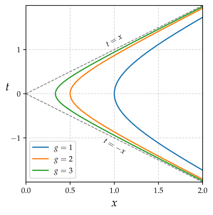
Figure 1: Trajectories given by (28) for different values of $g$.

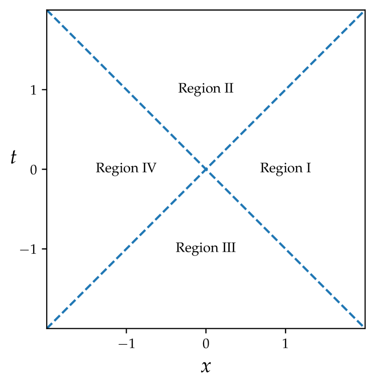
Figure 2: Four regions in Minkowski space-time.

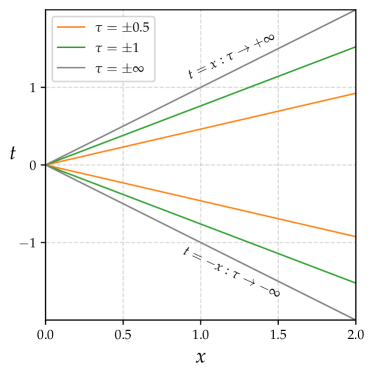
Figure 3: Foliations at $\tau=\pm 0.5,\pm 1$ and $\pm\infty$ for $g=1$.

2.1.2 Rindler coordinates

Although the transformations in (28) only give us the trajectory of the accelerated observer, we can use those in order to obtain a complete non-inertial perspective. That is to say, we need a spatial coordinate $\xi$ which, together with $\tau$, enables us to describe any physical phenomena in such a system, which will be called Rindler coordinates.

Let us start expressing the hyperbolic transformations (28) in exponential terms

$$x = \frac{1}{2}\left(\frac{e^{g\tau}}{g}+\frac{e^{-g\tau}}{g}\right)$$ (35)

$$t = \frac{1}{2}\left(\frac{e^{g\tau}}{g}-\frac{e^{-g\tau}}{g}\right)$$ (36)

Using null coordinates (Appendix A) for $(t,x)$

$$\overline{v} = t+x$$ (37)

$$\overline{u} = t-x$$ (38)

From (35) and (36), we obtain

$$\overline{v} = \frac{e^{g\tau}}{g}$$ (39)

$$\overline{u} = -\frac{e^{-g\tau}}{g}$$ (40)

Solving $\tau$ from (39) and (40) and adding these terms we obtain

$$\tau=\frac{\frac{1}{g}\ln{(\overline{v}g)}+\left(-\frac{1}{g}\ln{(-\overline{u}g)}\right)}{2}$$ (41)

Let us set $\xi$ as the spatial coordinate according to the accelerated frame. Therefore, we have the following null coordinates for $(\tau,\xi)$

$$v = \tau+\xi$$ (42)

$$u = \tau-\xi$$ (43)

Solving for $\tau$ and $\xi$ we obtain

$$\tau = \frac{v+u}{2}$$ (44)

$$\xi = \frac{v-u}{2}$$ (45)

Associating each null coordinate in Minkowski and Rindler in equations (41) and (44), we have

$$\frac{1}{g}\ln{(\overline{v}g)}=v\quad\rightarrow\quad\overline{v}=\frac{1}{g}e^{gv}$$ (46)

$$-\frac{1}{g}\ln{(-\overline{u}g)}=u\quad\rightarrow\quad\overline{u}=-\frac{1}{g}e^{-gu}$$ (47)

Then

$$t+x=\frac{1}{g}e^{g(\tau+\xi)}$$ (48)

$$t-x=-\frac{1}{g}e^{-g(\tau-\xi)}$$ (49)

Solving for $t$ we obtain

$$t=\frac{1}{2}\left(\frac{1}{g}e^{g\tau+g\xi}-\frac{1}{g}e^{-g\tau+g\xi}\right)$$ (50)

$$t=\frac{e^{g\xi}}{g}\left(\frac{e^{g\tau}-e^{-g\tau}}{2}\right)$$ (51)

Solving for $x$ we obtain

$$x=\frac{1}{2}\left(\frac{1}{g}e^{g\tau+g\xi}+\frac{1}{g}e^{-g\tau+g\xi}\right)$$ (52)

$$x=\frac{e^{g\xi}}{g}\left(\frac{e^{g\tau}+e^{-g\tau}}{2}\right)$$ (53)

Therefore

$$\begin{split}t=\frac{e^{g\xi}}{g}\sinh{(g\tau)}\\ x=\frac{e^{g\xi}}{g}\cosh{(g\tau)}\end{split}$$ (54)

As before, these transformations are defined in the region I of Minkowski space-time (Figure 2). In Figure 4 we show the parametric curve $(t(\tau,\xi),x(\tau,\xi))$, which can also be written as

$$x=\sqrt{t^{2}+\frac{e^{2g\xi}}{g^{2}}}$$ (55)

where the observers at rest (fixed $\xi=\xi_{0}$) in Rindler space-time describe a hyperbolic trajectory (55) in Minkowski. In addition, the foliations at constant $\tau$ are given by the same expression obtained in (30): the asymptotic regions for the accelerated observer ($t=\pm x$) are reached at $\tau\rightarrow\pm\infty$ (Figure 3).

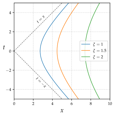
Figure 4: Trajectories given by (54) for different values of $\xi$ with $g=1$.

From (54) and (1) we obtain the line element of Rindler space-time

$$ds^{2}=e^{2g\xi}(-d\tau^{2}+d\xi^{2})$$ (56)

The line element (56) is complete in the sense that we can perform space-time measurements. In addition, since we have not imposed any restrictions on the Rindler coordinates $(\tau,\xi)$ in the transformation (54), these have the following ranges

$$-\infty<\tau<+\infty$$ (57)

$$-\infty<\xi<+\infty$$ (58)

Furthermore, the line element (56) is independent of $\tau$. Thus, $\partial_{\tau}$ is a Killing vector

$$\partial_{\tau} = \frac{\partial t}{\partial\tau}\partial_{t}+\frac{\partial x}{\partial\tau}\partial_{x}$$ (59)

$$\partial_{\tau} = g(x\partial_{t}+t\partial_{x})$$ (60)

that generates temporal translations in the Rindler space-time, while boost in Minkowski (Appendix B). In addition, it can be expressed as a contravariant vector in Minkowski space-time

$$\tau^{\mu}=(\tau^{0},\tau^{1})=(gx,gt)$$ (61)

with length given by

$$\tau^{\mu}\tau_{\mu}=-g^{2}x^{2}+g^{2}t^{2}=g^{2}(t+x)(t-x)$$ (62)

Such that, according to (31), (32), (33) and (34) we obtain

Region I $$:\tau^{\mu}\tau_{\mu}<0\,\,\,\,\,\,\,\,\rm{Time-like}$$ (63)

Region II $$:\tau^{\mu}\tau_{\mu}>0\,\,\,\,\,\,\,\,\rm{Space-like}$$ (64)

Region III $$:\tau^{\mu}\tau_{\mu}>0\,\,\,\,\,\,\,\,\rm{Space-like}$$ (65)

Region IV $$:\tau^{\mu}\tau_{\mu}<0\,\,\,\,\,\,\,\,\rm{Time-like}$$ (66)

On $x=\pm\,t$ we have $\tau^{\mu}\tau_{\mu}=0$. These regions are called killing horizons and correspond to $\tau\rightarrow\pm\infty$.

We can use this killing vector to determine in which direction the temporal coordinate $\tau$ evolves, according to Minkowski. It will confirm not only what we already know from (54), but also an important subtlety in region IV. For that purpose, we use the time basis vector in Minkowski

$$\partial_{t}\quad\rightarrow\quad t^{\mu}=(1,0)$$ (67)

which has been established, by definition, as future-directed, $t^{0}>0$, which is a global behavior due to the flat geometry of Minkowski.

As any future-directed vector (time-like or space-like) has a positive temporal component in its contravariant representation, its product with $t^{\mu}$ will give us a negative quantity. Therefore, $\tau^{\mu}$ will be future-directed if $\tau^{\mu}t_{\mu}<0$ and, past-directed if $\tau^{\mu}t_{\mu}>0$

$$\tau^{\mu}t_{\mu}=(gx,gt)\cdot(-1,0)=-gx$$ (68)

In region I, where $x>0$, $\tau$ and $t$ evolve in the same direction, as can be seen from the hyperbolic relation between $t$ and $\tau$ in (54). On the other hand, in region IV, where $x<0$, $\tau$ evolves in the opposite direction of $t$, the same feature is observed in the extended geometry of Schwarzschild. It suggests that region IV, in the light of the equivalence principle, may be seen as a time-reversed copy of region I. We will approach that behavior in the next section.

Finally, let us present an alternative form of the Rindler metric, which is more relevant for studying the black hole’s near-horizon geometry and its temperature. Let us define

$$\rho=\frac{e^{g\xi}}{g}$$ (69)

$$\omega=g\tau$$ (70)

Replacing (69) and (70) in (54) we obtain the following map to Minkowski

$$\begin{split}t=\rho\sinh{(\omega)}\\ x=\rho\cosh{(\omega)}\end{split}$$ (71)

From (71) and (1) we obtain an alternative version of the line element (56) for Rindler space-time

$$ds^{2}=-\rho^{2}d\omega^{2}+d\rho^{2}$$ (72)

where $\omega$ is dimensionless.

Comparing (69) and (70) with (57) and (58) we obtain the following ranges for Rindler coordinates $(\rho,\omega)$

$$0<\rho<+\infty$$ (73)

$$-\infty<\omega<+\infty$$ (74)

2.1.3 Extended geometry

We have built Rindler space-time from the analysis developed for the accelerated observer in Minkowski, from which we obtained that Rindler is only a portion of Minkowski, specifically region I. In addition, we obtained that in region IV of Minkowski, $\tau$ evolves in the opposite direction of $t$, thus, one may think that it contains a time-reversed copy of Rindler.

In this section, we will assume the existence of Rindler space-time independently of Minkowski, and we will analyze its extended geometry. Then, in order to reach our goal, we will analyze Rindler in analogy with Kruskal-Szekeres coordinates and then we will construct the Penrose-Carter diagram.

The metric associated with the line element (72) is singular at $\rho=0$ because its determinant vanishes at that point

$$g_{\mu\nu}=\begin{pmatrix}-\rho^{2}&0\\ 0&1\end{pmatrix}\quad,\quad g=\det{g_{\mu\nu}}=-\rho^{2}$$ (75)

Then, the inverse metric has a singular point at $\rho=0$, this is why we imposed $\rho>0$

$$g^{\mu\nu}=\begin{pmatrix}-\frac{1}{\rho^{2}}&0\\ 0&1\end{pmatrix}$$ (76)

To deal with this singularity, which is actually a coordinate singularity, and obtain a better understanding of the causal structure of Rindler space-time we need to introduce null coordinates. From the null condition for the line element

$$0=-\rho^{2}d\omega^{2}+d\rho^{2}$$ (77)

we obtain

$$\omega=\pm\ln{(\rho)}+const.$$ (78)

This gives us the following null coordinates

$$u=\omega-\ln{(\rho)}$$ (79)

$$v=\omega+\ln{(\rho)}$$ (80)

where $u$ and $v$ corresponds to out-going and in-going null geodesics respectively (Figures 6 and 6)

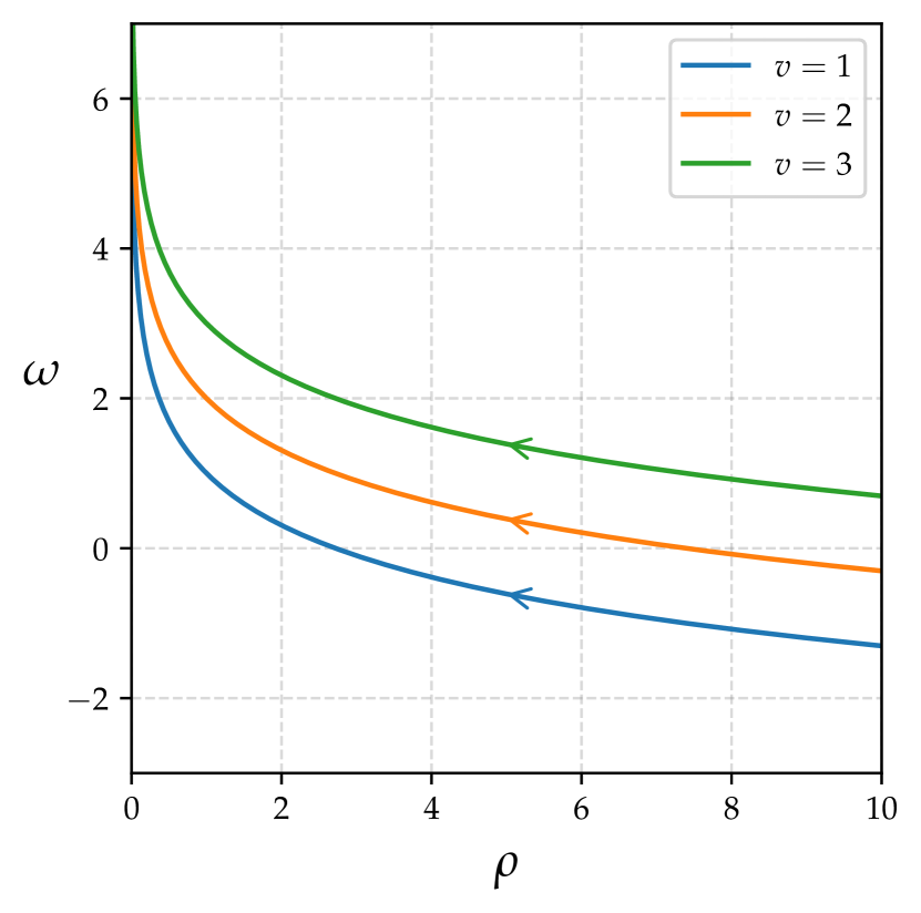
Figure 5: In-going null geodesics given by different values of $v$ according to equation (80).

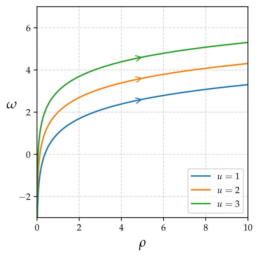
Figure 6: Out-going null geodesics given by different values of $u$ according to equation (79).

From (73) and (74) with (79) and (80) we obtain

$$-\infty<u<+\infty$$ (81)

$$-\infty<v<+\infty$$ (82)

In terms of the null coordinates $(u,v)$ given in (79) and (80), the line element (72) has the following form

$$ds^{2}=-e^{v-u}dudv$$ (83)

In (83), we still have a singularity in the coordinates due to the exponential term, which falls off when $v-u$ goes to $-\infty$, and precisely corresponds to the singularity at $\rho=0$, with $\omega=\omega_{o}$ finite, as can be seen from (79) and (80).

Let us return to the line element (72) and check that it is independent of $\omega$, which is the temporal coordinate, then there is a killing vector associated with the symmetry under temporal displacements

$$\omega^{\mu}=(1,0)$$ (84)

In addition, the conserved quantity due to this symmetry is the energy per unit mass

$$\varepsilon=-g_{\mu\nu}\omega^{\mu}\frac{d\rho^{\nu}}{d\lambda}$$ (85)

$$\varepsilon=\rho^{2}\frac{d\omega}{d\lambda}$$ (86)

where $\lambda$ is the affine parameter along the geodesic $\rho^{\nu}=(\omega,\rho)$. Let us examine the affine parameter for the out-going null geodesic, where $u=\textrm{constant}$. Then, from (79) and (80) we obtain

$$v-u=\ln{(\rho^{2})}\quad\rightarrow\quad\rho^{2}=e^{v-u}$$ (87)

$$\omega=\frac{u+v}{2}\quad\rightarrow\quad d\omega=\frac{dv}{2}$$ (88)

From (87) and (88) in (86) we obtain

$$\int d\lambda=\int\frac{e^{v-u}}{2\varepsilon}dv$$ (89)

$$\lambda=\frac{e^{v-u}}{2\varepsilon}\quad\rightarrow\quad\lambda=\left(\frac{e^{-u}}{2\varepsilon}\right)e^{v}$$ (90)

Since the term inside the parentheses on the right side of (90) is constant, we set $\lambda_{\textrm{out}}=e^{v}$ as the affine parameter on the out-going null geodesics.

In the same way, for the case of the affine parameter along the in-going geodesics, where $v=\textrm{constant}$, from (79) and (80), equation (88) now takes the following form

$$\omega=\frac{u+v}{2}\quad\rightarrow\quad d\omega=\frac{du}{2}$$ (91)

From (87) and (91) in (86) we obtain

$$\int d\lambda=\int\frac{e^{v-u}}{2\varepsilon}du$$ (92)

$$\lambda=-\frac{e^{v-u}}{2\varepsilon}\quad\rightarrow\quad\lambda=-e^{-u}\left(\frac{e^{v}}{2\varepsilon}\right)$$ (93)

Proceeding analogously, we set $\lambda_{\textrm{in}}=-e^{-u}$ as the affine parameter on the in-going null geodesics.

From (81) and (82) we obtain the following ranges for the affine parameters

$$-\infty<\lambda_{\textrm{in}}<0$$ (94)

$$0<\lambda_{\textrm{out}}<+\infty$$ (95)

which have a barrier in $\lambda_{\textrm{in}}=\lambda_{\textrm{out}}=0$ due to the singularity at $\rho=0$. Then, in order to avoid that singularity we define a new pair of null coordinates $(\bar{u},\bar{v})$ given by the affine parameters for in-going and out-going null geodesics $(\lambda_{\textrm{in}},\lambda_{\textrm{out}})$

$$\bar{u}(u)=\lambda_{\textrm{in}}\quad\rightarrow\quad\bar{u}=-e^{-u}$$ (96)

$$\bar{v}(v)=\lambda_{\textrm{out}}\quad\rightarrow\quad\bar{v}=e^{v}$$ (97)

From (94) and (95), we know that these null coordinates are restricted to $\bar{u}<0$ and $\bar{v}>0$. However, as the line element (83) is now given by

$$ds^{2}=-d\bar{u}d\bar{v}$$ (98)

where there is no longer any singularity, we can extend the geometry beyond the constraints imposed at $\bar{u}=\bar{v}=0$ in (94) and (95). Therefore

$$-\infty<\bar{u}<+\infty$$ (99)

$$-\infty<\bar{v}<+\infty$$ (100)

As $(\bar{u},\bar{v})$ are null coordinates, let us define them in the following way

$$\bar{u}=t-x$$ (101)

$$\bar{v}=t+x$$ (102)

Then, the line element (98) is now given by

$$ds^{2}=-dt^{2}+dx^{2}$$ (103)

This result tells us that Minkowski is the extended geometry of Rindler space-time, that is to say, Rindler is just a portion of Minkowski. In order to see exactly what this portion is we need to obtain the transformation between $(t,x)$ and $(\omega,\rho)$. From (79), (80), (101) and (102) in (96) and (97)

$$\bar{u}=-e^{-u}\quad\rightarrow\quad t-x=-e^{-\omega+\ln{(\rho)}}$$ (104)

$$\bar{v}=e^{v}\quad\rightarrow\quad t+x=e^{\omega+\ln{(\rho)}}$$ (105)

$$t=e^{\ln{(\rho)}}\left(\frac{e^{\omega}-e^{-\omega}}{2}\right)$$ (106)

$$x=e^{\ln{(\rho)}}\left(\frac{e^{\omega}+e^{-\omega}}{2}\right)$$ (107)

Therefore

$$\begin{split}t=\rho\sinh{(\omega)}\\ x=\rho\cosh{(\omega)}\end{split}$$ (108)

Which is precisely the transformation (71), and, as we already know, it covers the region I of Minkowski space-time (Figure 2). In that sense, the trajectories of a Rindler observer can be seen in the extended geometry as

$$x=\sqrt{t^{2}+\rho^{2}}$$ (109)

and the foliations at constant $\omega$ are given by the following expression

$$\frac{t}{x}=\tanh{(\omega)}$$ (110)

such that the asymptotic regions for Rindler observer, given by $t=\pm x$, corresponds to $\omega\rightarrow\pm\infty$ or $\rho=0\rightarrow\bar{u}=\bar{v}=0$. All these observations are shown in Figure 8.

Other important features are that the causal structure of the extended geometry of Rindler space-time is given by $45^{\circ}$ light-cones, which after being introduced give us that regions I and IV are causally disconnected (Figure 8). Also, all time-like geodesic remains within the light cones, while null-like geodesics are represented by $45^{\circ}$ straight lines (Figure 10).

As $\omega$ evolves in opposite directions in regions I and IV (Figure 8), which is the same feature observed in the extended geometry of Schwarzschild due to Kruskal-Szekeres coordinates, and $x<0$ in region IV, we may say that we have a time-reversed copy of the original Rindler space-time, as we have deduced in the previous section. Therefore, in region IV the coordinate transformation is given by

$$\begin{split}t=-\rho\sinh{(\omega)}\\ x=-\rho\cosh{(\omega)}\end{split}$$ (111)

Moreover, regions II and III are causally analogous to black and white holes, respectively, with horizons on $x=\pm t$, which corresponds to $\omega\rightarrow\pm\infty$ or $\rho=0$ (Figure 8).

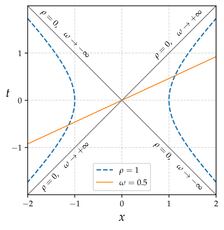
Figure 7: Trajectories for a constant $\rho$ and a foliation for a finite $\omega$.

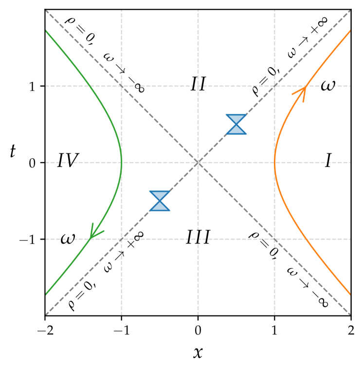
Figure 8: Causal structure of the extended geometry of Rindler space-time.

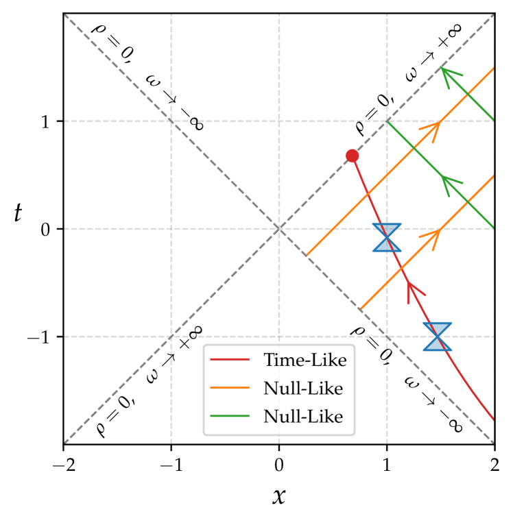
Figure 9: Time and Null-like geodesics of the Rindler observer in the $tx$-plane.

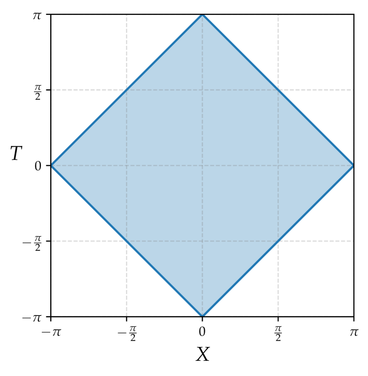
Figure 10: Region delimited by the ranges of $\quantity{\tilde{u},\tilde{v}}$ in the $TX$-plane.

We can summarize the whole extended geometry of Rindler space-time in a finite-range diagram, namely Penrose-Carter. Using the following maps will allow us to make finite the infinity

$$\bar{u}=\tan{\frac{\tilde{u}}{2}}$$ (112)

$$\bar{v}=\tan{\frac{\tilde{v}}{2}}$$ (113)

Which, from the extended geometry expressed in (99) and (100) gives us the following ranges for $\quantity(\tilde{u},\tilde{v})$

$$-\pi< \tilde{u} <\pi$$ (114)

$$-\pi< \tilde{v} <\pi$$ (115)

In these new coordinates the line element (98) is given by

$$ds^{2}=-\frac{1}{4}\sec^{2}{\frac{\tilde{u}}{2}}\sec^{2}{\frac{\tilde{v}}{2}}d\tilde{u}d\tilde{v}$$ (116)

Due to the ranges of $\quantity(\tilde{u},\tilde{v})$ in (114) and (115), we identify the conformal factor

$$\Omega=\frac{1}{2}\sec{\frac{\tilde{u}}{2}}\sec{\frac{\tilde{v}}{2}}>0$$ (117)

Thus

$$ds^{2}=\Omega^{2}d\tilde{s}^{2}$$ (118)

As both metrics are related by the conformal factor $\Omega$, then null geodesics are preserved (Appendix C). Therefore the metric with line element $ds^{2}$ has the same causal structure as that with $d\tilde{s}^{2}$. Defining $\quantity(\tilde{u},\tilde{v})$ as null coordinates

$$\tilde{u} = T-X$$ (119)

$$\tilde{v} = T+X$$ (120)

give us that the line element (72) is conformal to

$$d\tilde{s}^{2}=-dT^{2}+dX^{2}$$ (121)

In consequence, the causal structure is given by $45^{\circ}$ light-cones.

Now we are able to map the entire extended geometry in a finite region of the $TX$-plane, delimited by (114) and (115) (Figure 10) in what we know as the Penrose-Carter diagram (Figure 11).

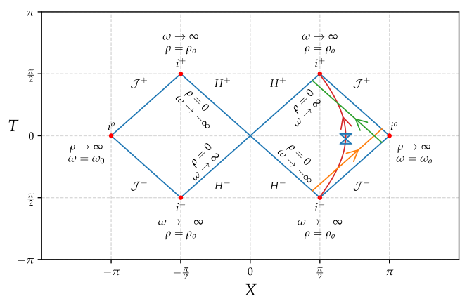
Figure 11: Penrose-Carter diagram of Rindler space-time.

As we know from (109), $\rho=0$ corresponds to $t=\pm x$ , which is the same as $\bar{u}=\bar{v}=0$. Then, from (112) and (113), we obtain that it also corresponds to $\tilde{u}=\tilde{v}=0$, which is the same as $T=\pm X$. Those asymptotic regions can be seen as horizons since the Rindler observer will reach those at $\omega\rightarrow\pm\infty$ (as shown in (110)) and nothing can get out from region II or get into region III. Moreover, the identification of the future $H^{+}$ and past horizons $H^{-}$ depends on the null rays, which travel in $45^{\circ}$ straight lines in the $TX$-plane. It means that null rays travel from the past null infinity $\mathcal{J}^{-}$ to the future horizon $H^{+}$ (green line in Figure 11), and from the past horizon $H^{-}$ to the future null infinity $\mathcal{J}^{+}$ (orange line in Figure 11). We also apply this procedure on the copy of Rindler space-time located on the left part of Figure 11.

In order to find the future and past time-like infinity, we analyze what happens at $\omega\rightarrow\pm\infty$ (future: $+$, past: $-$) with $\rho=\rho_{o}$ (finite) in equations (79), (80), (96), (97), (112) and (113).

Future time-like infinity $i^{+}$:

$$u\rightarrow\infty\quad\rightarrow\quad\bar{u}=0\quad\rightarrow\quad\tilde{u}=0\quad\rightarrow\quad T=X$$ (122)

$$v\rightarrow\infty\quad\rightarrow\quad\bar{v}\rightarrow\infty\quad\rightarrow\quad\tilde{v}=\pi\quad\rightarrow\quad T=-X+\pi$$ (123)

As both equations must be satisfied, the location of the future time-like infinity is given by the intersection of $\quantity{T=X,T=-X+\pi}$: $i^{+}=(\frac{\pi}{2},\frac{\pi}{2})$. As we know, in the left part of Figure 11 we have a copy of Rindler space-time, then, the future time-like infinity for that copy is located symmetrically: $i^{+}=(-\frac{\pi}{2},\frac{\pi}{2})$.

Past time-like infinity $i^{-}$:

$$u\rightarrow-\infty\quad\rightarrow\quad\bar{u}=-\infty\quad\rightarrow\quad\tilde{u}=-\pi\quad\rightarrow\quad T=X-\pi$$ (124)

$$v\rightarrow-\infty\quad\rightarrow\quad\bar{v}=0\quad\rightarrow\quad\tilde{v}=0\quad\rightarrow\quad T=-X$$ (125)

As before, the location of the past time-like infinity is given by the intersection of $\quantity{T=X-\pi,T=-X}$: $i^{-}=(\frac{\pi}{2},-\frac{\pi}{2})$. In consequence, in the copy of Rindler space-time, we have $i^{-}=(-\frac{\pi}{2},-\frac{\pi}{2})$.

Finally, in order to obtain space-like infinity, $i^{o}$, we apply $\omega=\omega_{o}$ (finite) with $\rho\rightarrow\infty$ in equations (79), (80), (96), (97), (112) and (113).

$$u\rightarrow-\infty\quad\rightarrow\quad\bar{u}=-\infty\quad\rightarrow\quad\tilde{u}=-\pi\quad\rightarrow\quad T=X-\pi$$ (126)

$$v\rightarrow\infty\quad\rightarrow\quad\bar{v}\rightarrow\infty\quad\rightarrow\quad\tilde{v}=\pi\quad\rightarrow\quad T=-X+\pi$$ (127)

Then, the location of the space-like infinity is given by the intersection of the lines $\quantity{T=X-\pi,T=-X+\pi}$: $i^{o}=(\pi,0)$. Clearly, in the copy of Rindler space-time, we have $i^{o}=(-\pi,0)$.

2.2 Free scalar field and the Bogoliubov-Valatin transformations

2.2.1 Scalar field and conformal transformation

The action for the real massive scalar field in $1+1$ background with metric $g_{\mu\nu}$ is given by

$$I=\int d^{2}x\sqrt{-g}\mathcal{L}=\int d^{2}x\sqrt{-g}\quantity[-\frac{1}{2}g^{\mu\nu}\nabla_{\mu}\phi\nabla_{\nu}\phi-V(\phi)]$$ (128)

where $V(\phi)=\frac{m^{2}}{2}\phi^{2}$. The equation of motion is obtained by taking the variation with respect to the field

$$\delta I=\int d^{4}x\sqrt{-g}\quantity[-g^{\mu\nu}\nabla_{\mu}\phi\delta\nabla_{\nu}\phi-\delta V\quantity(\phi)]$$ (129)

Using $\quantity[\nabla,\delta]=0$ and integrating by parts we obtain

$$\delta I=\int d^{4}x\sqrt{-g}\quantity[-\nabla^{\mu}\quantity(\nabla_{\mu}\phi\delta\phi)+g^{\mu\nu}\quantity(\nabla_{\mu}\nabla_{\nu}\phi)\delta\phi-\frac{dV}{d\phi}\delta\phi]$$ (130)

The first term in the bracket is a total derivative, applying Stoke’s theorem and the fact that the variation of the field is zero at the boundaries (infinity) we may neglect that term

$$\delta I=\int d^{4}x\sqrt{-g}\quantity[g^{\mu\nu}\quantity(\nabla_{\mu}\nabla_{\nu}\phi)-\frac{dV}{d\phi}]\delta\phi$$ (131)

From the variational principle, $\delta I=0$, and $\quantity[\nabla_{\mu},g^{\mu\nu}]=0$, we obtain

$$\nabla_{\mu}\quantity(g^{\mu\nu}\nabla_{\nu}\phi)=\frac{dV}{d\phi}$$ (132)

Using the well-known expression of the covariant derivative and the contraction of the Christoffel symbol we arrive to

$$\nabla_{\mu}\quantity(g^{\mu\nu}\nabla_{\nu}\phi) =\partial_{\mu}\quantity(g^{\mu\nu}\nabla_{\nu}\phi)+\Gamma^{\mu}_{\mu\nu}g^{\nu\alpha}\nabla_{\alpha}\phi$$ (133)

$$\Gamma^{\mu}_{\mu\nu} =\frac{1}{2}g^{\mu\alpha}\partial_{\nu}g_{\mu\alpha}$$ (134)

The expression for the Christoffel symbol used above may be written in a different form using the following property for a diagonalizable and invertible matrix $M$

$$\ \ln\quantity(\det M)=\Tr\quantity(\ln M)$$ (135)

Taking the derivative of the above expression

$$\partial_{\mu}\quantity(\ln\quantity(\det M))=\partial_{\mu}(\Tr\quantity(\ln M))$$ (136)

$$\frac{1}{\det M}\partial_{\mu}\quantity(\det M)=\Tr\partial_{\mu}(\ln M)=\Tr\quantity(M^{-1}\partial_{\mu}M)$$ (137)

and making $M=g_{\mu\nu}$ we obtain

$$\frac{1}{g}\partial_{\nu}g=g^{\mu\alpha}\partial_{\nu}g_{\mu\alpha}$$ (139)

Then, the Christoffel symbol (134) is given by

$$\Gamma^{\mu}_{\mu\nu}=\frac{1}{2g}\partial_{\nu}g=\frac{1}{\sqrt{-g}}\partial_{\nu}\sqrt{-g}$$ (140)

Finally, from (132), (133) and (140) we obtain the following form of the equation of motion for the scalar field $\phi$

$$\partial_{\mu}\quantity(g^{\mu\nu}\nabla_{\nu}\phi)+\frac{1}{\sqrt{-g}}\partial_{\mu}\quantity(\sqrt{-g})g^{\mu\nu}\nabla_{\nu}\phi=\frac{dV}{d\phi}$$ (141)

$$\frac{1}{\sqrt{-g}}\partial_{\mu}\quantity(\sqrt{-g}g^{\mu\nu}\nabla_{\nu}\phi)=\frac{dV}{d\phi}$$ (142)

A remarkable feature of the action (128) is that for $m=0$, it is invariant under the conformal transformation of the metric

$$\tilde{g}_{\mu\nu}=\Omega^{2}g_{\mu\nu}\rightarrow\tilde{g}^{\mu\nu} = \Omega^{-2}g^{\mu\nu}$$ (143)

$$\sqrt{-\tilde{g}} = \Omega^{2}\sqrt{-g}$$ (144)

$$\tilde{I}=-\frac{1}{2}\int d^{2}x\sqrt{-\tilde{g}}\tilde{g}^{\mu\nu}\nabla_{\mu}\phi\nabla_{\nu}\phi=-\frac{1}{2}\int d^{2}x\Omega^{2}\sqrt{-g}\Omega^{-2}g^{\mu\nu}\nabla_{\mu}\phi\nabla_{\nu}\phi=I$$ (145)

From Part 2.1, we know that the Rindler metric is conformal to that in Minkowski, with $\Omega^{2}=e^{2g\xi}$. Therefore, in Minkowski $(t,x)$ and Rindler $(\tau,\xi)$ we obtain the same form of the equation of motion

$$\Box\phi(t,x)=\Box\phi(\tau,\xi)=0$$ (146)

2.2.2 Fourier modes and inner product

The real scalar field operator $\phi(x^{\mu})$ (where $x^{\mu}=(t,x)$ or $x^{\mu}=(\tau,\xi)$) can be expressed in terms of Fourier modes

$$\phi(x^{\mu})=\int_{-\infty}^{\infty}\frac{dk}{\sqrt{4\pi\omega_{k}}}(a(k)e^{ik^{\mu}x_{\mu}}+a^{\dagger}(k)e^{-ik^{\mu}x_{\mu}})$$ (147)

where $k^{\mu}=(k^{0},k)$, and $k^{0}=\omega_{k}=\sqrt{k^{2}+m^{2}}$.

As we know, $a^{\dagger}(k)$ and $a(k)$ satisfy the following commutation rules

$$\left[a(k),a^{\dagger}(k^{\prime})\right]=\delta(k-k^{\prime})$$ (148)

$$\left[a(k),a(k^{\prime})\right]=\left[a^{\dagger}(k),a^{\dagger}(k^{\prime})\right]=0$$ (149)

In addition, at quantum level we obtain the same equation of motion for the field operator in Minkowski and Rindler space-time (146).

Splitting the expression (147) for $k>0$ and $k<0$, we obtain

$$\phi(x^{\mu})=\int_{0}^{\infty}\frac{dk}{\sqrt{4\pi\omega_{k}}}(a(k)e^{ik^{\mu}x_{\mu}}+a^{\dagger}(k)e^{-ik^{\mu}x_{\mu}})\\ +\int_{-\infty}^{0}\frac{dk}{\sqrt{4\pi\omega_{k}}}(a(k)e^{ik^{\mu}x_{\mu}}+a^{\dagger}(k)e^{-ik^{\mu}x_{\mu}})$$ (150)

Changing $k\rightarrow-k$ in the second integral enables us to express the field operator in the following way

$$\phi(x^{\mu})=\int_{0}^{\infty}\frac{dk}{\sqrt{4\pi\omega_{k}}}(a(k)e^{i(-\omega_{k}t+kx)}+a^{\dagger}(k)e^{-i(-\omega_{k}t+kx)}\\ +b(k)e^{i(-\omega_{k}t-kx)}+b^{\dagger}(k)e^{-i(-\omega_{k}t-kx)})$$ (151)

where $b(k)=a(-k)$.

In what follows, we will consider a massless field, $m_{\phi}=0$, for which

$$\omega_{k}=\absolutevalue{k}=\omega>0$$ (152)

In addition, due to the conformal invariance, the field operator in Minkowski and Rindler (regions I and IV) can be expressed as follows

$$\phi(t,x)=\int_{0}^{\infty}d\omega(a(\omega)f_{\omega}+a^{\dagger}(\omega)f^{*}_{\omega}+b(\omega)g_{\omega}+b^{\dagger}(\omega)g^{*}_{\omega})$$ (153)

$$\phi(\tau,\xi)=\int_{0}^{\infty}d\omega(c(\omega)h_{\omega}+c^{\dagger}(\omega)h^{*}_{\omega}+d(\omega)j_{\omega}+d^{\dagger}(\omega)j^{*}_{\omega})$$ (154)

In both fields the creation and annihilation operators $\quantity{a_{\omega},a^{\dagger}_{\omega},b_{\omega},b^{\dagger}_{\omega},c_{\omega},c^{\dagger}_{\omega},d_{\omega},d^{\dagger}_{\omega}}$ satisfy the commutation rules (148) and (149).

The Fourier modes in (153) and (154) are given by

$$f_{\omega}=\frac{e^{-i\omega(t-x)}}{\sqrt{4\pi\omega}}$$ (155)

$$g_{\omega}=\frac{e^{-i\omega(t+x)}}{\sqrt{4\pi\omega}}$$ (156)

$$h_{\omega}=\frac{e^{-i\omega(\tau-\xi)}}{\sqrt{4\pi\omega}}$$ (157)

$$j_{\omega}=\frac{e^{-i\omega(\tau+\xi)}}{\sqrt{4\pi\omega}}$$ (158)

The $f_{\omega}$ and $g_{\omega}$ modes are identified as right and left modes, respectively (the same for $h_{\omega}$ and $j_{\omega}$). In addition, each of them represents a complete basis for the field operator, and satisfies the Klein-Gordon inner product, as presented by Wald in [5]

$$\langle\mathcal{F}_{\omega},\mathcal{F}_{\omega^{\prime}}\rangle:=-i\int_{\Sigma}\sqrt{\sigma}d\Sigma^{\mu}\quantity[\mathcal{F}_{\omega^{\prime}}\nabla_{\mu}\mathcal{F}^{*}_{\omega}-\mathcal{F}^{*}_{\omega}\nabla_{\mu}\mathcal{F}_{\omega^{\prime}}]$$ (159)

where $d\Sigma^{\mu}=d\Sigma n^{\mu}$, and $\Sigma$ is a Cauchy surface.

Considering $\Sigma$ given by $S=x^{0}-x_{\circ}^{0}=0$, the normal vector $n^{\mu}$ (see for example Appendix D of [6]) is defined as follows

$$n^{\mu} = -\frac{\zeta^{\mu}}{\absolutevalue{\zeta^{\mu}\zeta_{\mu}}^{1/2}}$$ (160)

$$\zeta^{\mu} = g^{\mu\nu}\nabla_{\nu}S$$ (161)

For Minkowski (1) and Rindler metric (56) we have

$$\textrm{Minkowski}: n^{\mu} =\delta^{\mu}_{0}\,\,,\,\,\sqrt{\sigma}=1\,\,,\,\,d\Sigma=dx\rightarrow\sqrt{\sigma}d\Sigma^{\mu}=dx\delta^{\mu}_{0}$$ (162)

$$\textrm{Rindler}: n^{\mu} =e^{-g\xi}\delta^{\mu}_{0}\,\,,\,\,\sqrt{\sigma}=e^{g\xi}\,\,,\,\,d\Sigma=d\xi\rightarrow\sqrt{\sigma}d\Sigma^{\mu}=d\xi\delta^{\mu}_{0}$$ (163)

From the inner product (159), the differential surface vectors (162) and (163), and the Fourier modes (155), (156), (157) and (158), we have

$$\langle f_{\omega},f_{\omega^{\prime}}\rangle=\langle g_{\omega},g_{\omega^{\prime}}\rangle = \delta(\omega-\omega^{\prime})$$ (164)

$$\langle f^{*}_{\omega},f_{\omega^{\prime}}\rangle=\langle g^{*}_{\omega},g_{\omega^{\prime}}\rangle = 0$$ (165)

$$\langle h_{\omega},h_{\omega^{\prime}}\rangle=\langle j_{\omega},j_{\omega^{\prime}}\rangle = \delta(\omega-\omega^{\prime})$$ (166)

$$\langle h^{*}_{\omega},h_{\omega^{\prime}}\rangle=\langle j^{*}_{\omega},j_{\omega^{\prime}}\rangle = 0$$ (167)

The left and right modes are orthogonal to each other

$$\langle f_{\omega},g_{\omega^{\prime}}\rangle=\langle f^{*}_{\omega},g_{\omega^{\prime}}\rangle=0$$ (168)

$$\langle h_{\omega},j_{\omega^{\prime}}\rangle=\langle h^{*}_{\omega},j_{\omega^{\prime}}\rangle=0$$ (169)

Furthermore, the complex conjugate of the inner product (159) satisfies the following property

$${\langle\mathcal{F}_{\omega},\mathcal{G}_{\omega^{\prime}}\rangle}^{*}=-\langle\mathcal{F}^{*}_{\omega},\mathcal{G}^{*}_{\omega^{\prime}}\rangle=\langle\mathcal{G}_{\omega^{\prime}},\mathcal{F}_{\omega}\rangle$$ (170)

2.2.3 Bogoliubov-Valatin transformation

Let us define the null coordinates $\quantity{\bar{u},\bar{v},u,v}$ in Minkowski $(t,x)$ and Rindler $(\tau,\xi)$

$$\bar{u}=t-x$$ (171)

$$\bar{v}=t+x$$ (172)

$$u=\tau-\xi$$ (173)

$$v=\tau+\xi$$ (174)

Then, the equations of motion (146) are now expressed as follows

$$\partial_{\bar{u}}\partial_{\bar{v}}\phi = 0$$ (175)

$$\partial_{u}\partial_{v}\phi = 0\,$$ (176)

for the scalar field in Minkowski and Rindler null coordinates, respectively.

Evidently, by virtue of (175) and (176), each solution is of the form

$$\phi(\bar{u},\bar{v})=\phi(\bar{u})+\phi(\bar{v})$$ (177)

$$\phi(u,v)=\phi(u)+\phi(v)$$ (178)

It means that $\phi(\bar{u})$ and $\phi(\bar{v})$ are decoupled, which is in agreement with what we obtained in (168) and (169). Let us write the decoupled Fourier modes, (155) and (156), in null coordinates

$$f_{\omega}=\frac{e^{-i\omega\bar{u}}}{\sqrt{4\pi\omega}}$$ (179)

$$g_{\omega}=\frac{e^{-i\omega\bar{v}}}{\sqrt{4\pi\omega}}$$ (180)

Expanding $\phi(\bar{u})$ and $\phi(\bar{v})$ in those basis

$$\phi(\bar{u})=\int_{0}^{\infty}d\omega(a(\omega)f_{\omega}+a^{\dagger}(\omega)f^{*}_{\omega})$$ (181)

$$\phi(\bar{v})=\int_{0}^{\infty}d\omega(b(\omega)g_{\omega}+b^{\dagger}(\omega)g^{*}_{\omega})$$ (182)

Adding the above expressions we obtain (177), which, as expected, is equal to (153).

The same procedure is applied to Rindler modes (157) and (158)

$$h_{\omega}=\frac{e^{-i\omega u}}{\sqrt{4\pi\omega}}$$ (183)

$$j_{\omega}=\frac{e^{-i\omega v}}{\sqrt{4\pi\omega}}$$ (184)

From (178) we obtain the decoupled fields

$$\phi(u)=\int_{0}^{\infty}d\omega(c(\omega)h_{\omega}+c^{\dagger}(\omega)h^{*}_{\omega})$$ (185)

$$\phi(v)=\int_{0}^{\infty}d\omega(d(\omega)j_{\omega}+d^{\dagger}(\omega)j^{*}_{\omega})$$ (186)

As before, the sum of them reproduce (178) and (154).

The right modes in Minkowski and Rindler are related by the Bogoliubov-Valatin transformation [7][8]

$$h_{\omega^{\prime}}=\int_{0}^{\infty}d\Omega(\alpha_{\omega^{\prime}\Omega}f_{\Omega}+\beta_{\omega^{\prime}\Omega}f^{*}_{\Omega})$$ (187)

The coefficients $\alpha_{\omega^{\prime}\Omega}$ and $\beta_{\omega^{\prime}\Omega}$ are obtained by the Klein-Gordon inner product

$$\langle h_{\omega^{\prime}},f_{\omega}\rangle = \alpha_{\omega^{\prime}\omega}$$ (188)

$$\langle h_{\omega^{\prime}},f^{*}_{\omega}\rangle = -\beta_{\omega^{\prime}\omega}$$ (189)

Applying the property (170) we obtain

$$\langle f_{\omega},h_{\omega^{\prime}}\rangle = \alpha^{*}_{\omega^{\prime}\omega}$$ (190)

$$\langle f_{\omega},h^{*}_{\omega^{\prime}}\rangle = \beta_{\omega^{\prime}\omega}$$ (191)

Thus, we can write the right mode in Minkowski in terms of that in Rindler

$$f_{\omega}=\int_{0}^{\infty}d\Omega(\alpha^{*}_{\Omega\omega}h_{\Omega}-\beta_{\Omega\omega}h^{*}_{\Omega})$$ (192)

From the equality between the right modes in Minkowski and Rindler $\quantity{\phi(\bar{u}),\phi(u)}$ (the same analysis for $\quantity{\phi(\bar{v}),\phi(v)}$)

$$\int_{0}^{\infty}d\omega(a(\omega)f_{\omega}+a^{\dagger}(\omega)f^{*}_{\omega})=\int_{0}^{\infty}d\omega^{\prime}(c(\omega^{\prime})h_{\omega^{\prime}}+c^{\dagger}(\omega^{\prime})h^{*}_{\omega^{\prime}})\,$$ (193)

Then, using (192) in (193)

$$\int_{0}^{\infty}d\omega(a(\omega)f_{\omega}+a^{\dagger}(\omega)f^{*}_{\omega})=\int_{0}^{\infty}d\omega a(\omega)\displaystyle\int_{0}^{\infty}d\Omega(\alpha^{*}_{\Omega\omega}h_{\Omega}-\beta_{\Omega\omega}h^{*}_{\Omega})\\ +\int_{0}^{\infty}d\omega a^{\dagger}(\omega)\displaystyle\int_{0}^{\infty}d\Omega(\alpha_{\Omega\omega}h^{*}_{\Omega}-\beta^{*}_{\Omega\omega}h_{\Omega})$$

Rearranging and comparing term by term with the right-hand side of (193)

$$\int_{0}^{\infty}d\Omega\displaystyle\int_{0}^{\infty}d\omega(\alpha^{*}_{\Omega\omega}a(\omega)-\beta^{*}_{\Omega\omega}a^{\dagger}(\omega))h_{\Omega}\\ +\int_{0}^{\infty}d\Omega\displaystyle\int_{0}^{\infty}d\omega(\alpha_{\Omega\omega}a^{\dagger}(\omega)-\beta_{\Omega\omega}a(\omega))h^{*}_{\Omega}=\int_{0}^{\infty}d\Omega(c(\Omega)h_{\Omega}+c^{\dagger}(\Omega)h^{*}_{\Omega})$$

We obtain the annihilation operator in Rindler in terms of the annihilation and creation operators in Minkowski

$$c(\Omega)=\int_{0}^{\infty}d\omega(\alpha^{*}_{\Omega\omega}a(\omega)-\beta^{*}_{\Omega\omega}a^{\dagger}(\omega))$$ (194)

Similarly, using (187) in (193), we obtain the analogous result

$$a(\omega)=\int_{0}^{\infty}d\Omega(\alpha_{\Omega\omega}c(\Omega)+\beta^{*}_{\Omega\omega}c^{\dagger}(\Omega))$$ (195)

Finally, using (192) in (187)

$$h_{\omega^{\prime}}=\int_{0}^{\infty}d\Omega\alpha_{\omega^{\prime}\Omega}\displaystyle\int_{0}^{\infty}d\omega(\alpha^{*}_{\omega\Omega}h_{\omega}-\beta_{\omega\Omega}h^{*}_{\omega})+\int_{0}^{\infty}d\Omega\beta_{\omega^{\prime}\Omega}\displaystyle\int_{0}^{\infty}d\omega(\alpha_{\omega\Omega}h^{*}_{\omega}-\beta^{*}_{\omega\Omega}h_{\omega})\,$$

we obtain the following properties for the Bogoliubov-Valatin coefficients

$$\int_{0}^{\infty}d\Omega(\alpha_{\omega^{\prime}\Omega}\alpha^{*}_{\omega\Omega}-\beta_{\omega^{\prime}\Omega}\beta^{*}_{\omega\Omega}) = \delta(\omega-\omega^{\prime})$$ (196)

$$\alpha_{\omega^{\prime}\Omega}\beta_{\omega\Omega} = \beta_{\omega^{\prime}\Omega}\alpha_{\omega\Omega}$$ (197)

3 Part II - The Unruh effect

As we saw in the previous section, we can express the creation and annihilation operators of the field in Rindler space-time in terms of those in Minkowski (194). Therefore, the number operator for an arbitrary energy $\omega$ for right modes in the right wedge (region I) of the Rindler space-time

$$N_{R}(\omega)=c^{\dagger}(\omega)c(\omega)$$ (198)

acts on the energy states of the field in Minkowski. In what follows we will explore the perception of the observer under constant acceleration with respect to the ground state of the field in Minkowski space-time.

$$\matrixelement{0_{M}}{N_{R}(\omega)}{0_{M}}=\matrixelement{0_{M}}{c^{\dagger}(\omega)c(\omega)}{0_{M}}$$ (199)

Using (194) in the above expression

$$\matrixelement{0_{M}}{N_{R}(\omega)}{0_{M}}=\bra{0_{M}}\int_{0}^{\infty}d\Omega^{\prime}(\alpha_{\omega\Omega^{\prime}}a^{\dagger}(\Omega^{\prime})-\beta_{\omega\Omega^{\prime}}a(\Omega^{\prime}))\\ \int_{0}^{\infty}d\Omega(\alpha^{*}_{\omega\Omega}a(\Omega)-\beta^{*}_{\omega\Omega}a^{\dagger}(\Omega))\ket{0_{M}}$$ (200)

Applying the action of the creation and annihilation operators in Minkowski over the ground state $\ket{0_{M}}$

$$a^{\dagger}(\Omega)\ket{0_{M}} = \ket{(1,\Omega)_{M}}$$ (201)

$$a(\Omega)\ket{0_{M}} = 0$$ (202)

we obtain the following expression

$$\matrixelement{0_{M}}{N_{R}(\omega)}{0_{M}}=\quantity[\int_{0}^{\infty}d\Omega^{\prime}\bra{(1,\Omega^{\prime})_{M}}\beta_{\omega\Omega^{\prime}}]\quantity[\int_{0}^{\infty}d\Omega\beta^{*}_{\omega\Omega}\ket{(1,\Omega)_{M}}]$$ (203)

Thus, what we obtain in (203) is just an infinite sum of $\absolutevalue{\beta_{\omega\Omega}}^{2}$, which is a positive quantity, over the whole energy spectrum $\Omega$ of the field in Minkowski (200)

$$\matrixelement{0_{M}}{N_{R}(\omega)}{0_{M}}=\int_{0}^{\infty}d\Omega\absolutevalue{\beta_{\omega\Omega}}^{2}$$ (204)

Then, it is expected to obtain a divergent value.

On the other hand, if we made the computation in (199) using the number operator with energy $\omega$ (for the right modes) in Minkowski, $N_{M}(\omega)$, instead of $N_{R}(\omega)$, we obtain

$$\matrixelement{0_{M}}{N_{M}(\omega)}{0_{M}}=\matrixelement{0_{M}}{a^{\dagger}(\omega)a(\omega)}{0_{M}}=0$$ (205)

As we see, the difference between (204) and (205) is due to the factor $\beta_{\Omega\omega}$, which is responsible for combining modes of positive and negative norm $\quantity{f_{\Omega},f^{*}_{\Omega}}$ (187). Thus, when $\beta_{\Omega\omega}=0$ the Rindler modes with positive and negative norm $\quantity{h_{\omega^{\prime}},h^{*}_{\omega^{\prime}}}$ are just superposition of their analogues in Minkowski

$$h_{\omega^{\prime}} = \int_{0}^{\infty}d\Omega(\alpha_{\omega^{\prime}\Omega}f_{\Omega})$$ (206)

$$h^{*}_{\omega^{\prime}} = \int_{0}^{\infty}d\Omega(\alpha^{*}_{\omega^{\prime}\Omega}f^{*}_{\Omega})$$ (207)

So, it is important to know the value of $\beta_{\Omega\omega}$ to understand its physical implication.

Let us start from (193), and using the values of $f_{\omega}$ and $h_{\omega^{\prime}}$ given in (179) and (183)

$$\int_{0}^{\infty}d\omega\quantity[a(\omega)\frac{e^{-i\omega\bar{u}}}{\sqrt{4\pi\omega}}+a^{\dagger}(\omega)\frac{e^{i\omega\bar{u}}}{\sqrt{4\pi\omega}}]=\int_{0}^{\infty}d\omega^{\prime}\quantity[c(\omega^{\prime})\frac{e^{-i\omega^{\prime}u}}{\sqrt{4\pi\omega^{\prime}}}+c^{\dagger}(\omega^{\prime})\frac{e^{i\omega^{\prime}u}}{\sqrt{4\pi\omega^{\prime}}}]$$ (208)

From the coordinate transformation (47) between Minkowski and Rindler we know that both sides of the expression (208) are functions of $u$. In that sense, we can apply the Fourier transformation in order to get them in terms of the energy $\Omega$

$$\int_{-\infty}^{\infty}\frac{du}{\sqrt{2\pi}}e^{i\Omega u}\int_{0}^{\infty}d\omega\quantity[a(\omega)\frac{e^{-i\omega\bar{u}}}{\sqrt{4\pi\omega}}+a^{\dagger}(\omega)\frac{e^{i\omega\bar{u}}}{\sqrt{4\pi\omega}}]=\\ \int_{-\infty}^{\infty}\frac{du}{\sqrt{2\pi}}e^{i\Omega u}\int_{0}^{\infty}d\omega^{\prime}\quantity[c(\omega^{\prime})\frac{e^{-i\omega^{\prime}u}}{\sqrt{4\pi\omega^{\prime}}}+c^{\dagger}(\omega^{\prime})\frac{e^{i\omega^{\prime}u}}{\sqrt{4\pi\omega^{\prime}}}]$$ (209)

Rearranging the right-hand side of the above expression

$$\int_{0}^{\infty}\frac{d\omega^{\prime}}{\sqrt{2\omega^{\prime}}}\quantity[c(\omega^{\prime})\int_{-\infty}^{\infty}\frac{du}{2\pi}e^{iu(\Omega-\omega^{\prime})}+c^{\dagger}(\omega^{\prime})\int_{-\infty}^{\infty}\frac{du}{2\pi}e^{iu(\Omega+\omega^{\prime})}]$$ (210)

and using the definition of the Dirac delta function

$$\delta(\Omega-\omega^{\prime})=\int_{-\infty}^{\infty}\frac{du}{2\pi}e^{iu(\Omega-\omega^{\prime})}$$ (211)

from (209) we obtain

$$c(\Omega)=\int_{0}^{\infty}d\omega\left[\quantity(\int_{-\infty}^{\infty}\frac{du}{2\pi}\sqrt{\frac{\Omega}{\omega}}e^{i(\Omega u-\omega\bar{u})})a(\omega)+\quantity(\int_{-\infty}^{\infty}\frac{du}{2\pi}\sqrt{\frac{\Omega}{\omega}}e^{i(\Omega u+\omega\bar{u})})a^{\dagger}(\omega)\right]$$ (212)

Comparing term by term with (194), and replacing the value of $\overline{u}(u)$ given in (47), we obtain the following expressions for the Bogoliubov-Valatin coefficients

$$\alpha^{*}_{\Omega\omega} = \sqrt{\frac{\Omega}{\omega}}\int_{-\infty}^{\infty}\frac{du}{2\pi}e^{i(\Omega u+\frac{\omega}{g}e^{-gu})}$$ (213)

$$\beta^{*}_{\Omega\omega} = -\sqrt{\frac{\Omega}{\omega}}\int_{-\infty}^{\infty}\frac{du}{2\pi}e^{i(\Omega u-\frac{\omega}{g}e^{-gu})}$$ (214)

The integrals on the right-hand side of the (213) and (214) can be solved by doing the following transformation

$$\gamma\frac{i\omega}{g}e^{-gu}=e^{x}$$ (215)

where $\gamma=\pm 1$. Thus, we obtain

$$u=-\frac{1}{g}\ln{\quantity(\frac{g}{\gamma i\omega})}-\frac{1}{g}x$$ (216)

from which we have that $du=-dx/g$, and $x\rightarrow\pm\infty$ for $u\rightarrow\mp\infty$. Therefore

$$\int_{-\infty}^{\infty}\frac{du}{2\pi}e^{i(\Omega u-\gamma\frac{\omega}{g}e^{-gu})}=\frac{e^{\frac{-\gamma\pi\Omega}{2g}}}{2\pi g}\quantity(\frac{g}{\omega})^{-\frac{i\Omega}{g}}\int_{-\infty}^{\infty}dxe^{-e^{x}}e^{\quantity(-\frac{i\Omega}{g})x}$$ (217)

Using the definition of the gamma function given by Nielsen in [9], we obtain

$$\alpha^{*}_{\Omega\omega}=\sqrt{\frac{\Omega}{\omega}}\frac{e^{\frac{\pi\Omega}{2g}}}{2\pi g}\quantity(\frac{g}{\omega})^{-\frac{i\Omega}{g}}\Gamma\quantity(-\frac{i\Omega}{g})$$ (218)

$$\beta^{*}_{\Omega\omega}=-\sqrt{\frac{\Omega}{\omega}}\frac{e^{-\frac{\pi\Omega}{2g}}}{2\pi g}\quantity(\frac{g}{\omega})^{-\frac{i\Omega}{g}}\Gamma\quantity(-\frac{i\Omega}{g})$$ (219)

Hence

$$\alpha^{*}_{\Omega\omega}=-e^{\frac{\Omega\pi}{g}}\beta^{*}_{\Omega\omega}$$ (220)

Using (220) in the property (196) of the Bogoliubov-Valatin coefficients

$$\delta(\Omega-\Omega^{\prime}) =\int_{0}^{\infty}d\omega\quantity(\alpha_{\Omega^{\prime}\omega}\alpha^{*}_{\Omega\omega}-\beta_{\Omega^{\prime}\omega}\beta^{*}_{\Omega\omega})$$ (221)

$$=\int_{0}^{\infty}d\omega\quantity(e^{\frac{\quantity(\Omega^{\prime}+\Omega)\pi}{g}}\beta_{\Omega^{\prime}\omega}\beta^{*}_{\Omega\omega}-\beta_{\Omega^{\prime}\omega}\beta^{*}_{\Omega\omega})$$ (222)

we arrive to

$$\frac{1}{e^{\frac{(\Omega^{\prime}+\Omega)\pi}{g}}-1}\delta(\Omega-\Omega^{\prime})=\int_{0}^{\infty}d\omega\beta_{\Omega^{\prime}\omega}\beta^{*}_{\Omega\omega}$$ (223)

Making $\Omega^{\prime}=\Omega$ we obtain a divergent integral, as we mentioned in (204). This result is due to the integration over the whole spectrum of energy $\omega$ for the scalar field in Minkowski. See equation (208).

In addition, the left-hand side of (223) is a density for a specific value of $\Omega$, which is the energy for the scalar field in Rindler

$$\matrixelement{0_{M}}{N_{R}(\Omega)}{0_{M}}=\frac{1}{e^{\frac{2\pi\Omega}{g}}-1}\delta(0)=\int_{0}^{\infty}d\omega\absolutevalue{\beta_{\Omega\omega}}^{2}$$ (224)

The quantity next to $\delta(0)$ is the particle number density $n_{R}(\Omega)$ for the right modes, in the right wedge of Rindler space-time, with respect to the ground state in Minkowski

$$n_{R}(\Omega)=\frac{1}{e^{\frac{2\pi\Omega}{g}}-1}$$ (225)

Therefore, the accelerated observer (in region I) describes the Minkowski ground state as a Bose-Einstein distribution for massless spin-0 particles (scalar field) with energy $E=\Omega$, and temperature proportional to its acceleration

$$n_{R}(E=\Omega)=\frac{1}{e^{\frac{2\pi\Omega}{g}}-1}=\frac{1}{e^{\frac{E}{T}}-1}$$ (226)

$$T=\frac{g}{2\pi}$$ (227)

This is the Unruh Effect, named after the Canadian physicist William G. Unruh [10].

4 Part III - Euclidean approach and the Thermofield Double State

4.1 Euclidean path integral

The transition amplitude due to the time evolution operator $e^{-iHt}$, given by

$$\innerproduct{\phi(x_{f},t_{f}=t)}{\phi(x_{\circ},t_{\circ}=0)}=\matrixelement{\phi_{f}}{e^{-iHt}}{\phi_{\circ}}$$ (228)

is expressed as a Feynman Path Integral

$$\matrixelement{\phi_{f}}{e^{-iHt}}{\phi_{\circ}}=\displaystyle\int_{\phi(t_{\circ})=\phi_{\circ}}^{\phi(t)=\phi_{f}}D\quantity[\phi]e^{iI\quantity[\phi]}$$ (229)

where the integration limits correspond to the initial and final states, and $I$ is the classical action of the theory: $I\quantity[\phi]=\int dtdx\mathcal{L}(\phi).$

Let us develop the above analysis in the Euclidean signature. To do that, we apply the Wick rotation

$$t_{E}=it$$ (230)

Thus, the transition amplitude is through the Euclidean time

$$\matrixelement{\phi_{f}}{e^{-Ht_{E}}}{\phi_{\circ}}$$ (231)

Applying (230) in $iI$, for the real scalar field $\phi$, we obtain

$$iI\quantity[\phi]=i\int dtdx\quantity[\frac{1}{2}\quantity(\frac{\partial\phi}{\partial t})^{2}-\frac{1}{2}\quantity(\nabla\phi)^{2}-\frac{1}{2}m^{2}\phi^{2}]\\ =-\int dt_{E}dx\quantity[\frac{1}{2}\quantity(\frac{\partial\phi}{\partial t_{E}})^{2}+\frac{1}{2}\quantity(\nabla\phi)^{2}+\frac{1}{2}m^{2}\phi^{2}]$$ (232)

the Euclidean action is given by

$$I_{E}\quantity[\phi]:=\int dt_{E}dx\quantity[\frac{1}{2}\quantity(\frac{\partial\phi}{\partial t_{E}})^{2}+\frac{1}{2}\quantity(\nabla\phi)^{2}+\frac{1}{2}m^{2}\phi^{2}]$$ (233)

As we note, the term in square brackets in (233) is the Hamiltonian density $\mathcal{H}$ for the Euclidean time $t_{E}$. Considering that $\mathcal{H}$ is time-independent, then

$$iI\quantity[\phi]=-I_{E}\quantity[\phi]=-HT$$ (234)

where

$$H = \int d\sigma\quantity[\frac{1}{2}\quantity(\frac{\partial\phi}{\partial t_{E}})^{2}+\frac{1}{2}\quantity(\nabla\phi)^{2}+\frac{1}{2}m^{2}\phi^{2}]$$ (235)

$$T = \int dt_{E}$$ (236)

Applying the Wick rotation (230) in the amplitude (229) we obtain

$$\matrixelement{\phi_{f}}{e^{-Ht_{E}}}{\phi_{\circ}}=\displaystyle\int_{\phi(t_{E}=0)=\phi_{\circ}}^{\phi(t_{E})=\phi_{f}}D\quantity[\phi]e^{-I_{E}\quantity[\phi]}$$ (237)

In addition, the state $\ket{\psi}$, propagated from $t_{E}=-T$ to $t_{E}=t=0$

$$\ket{\psi(t=0)}=e^{-HT}\ket{\psi(t_{E}=-T)}$$ (238)

is given by a Euclidean path integral without a defined upper limit

$$\ket{\psi(t=0)}=e^{-HT}\ket{\psi(t_{E}=-T)}=\displaystyle\int_{\psi(t_{E}=-T)=\psi_{\circ}}^{\psi(t=0)}D\quantity[\psi]e^{-I_{E}\quantity[\psi]}$$ (239)

In general, an arbitrary state at Lorentzian time $t$ can be seen as a result of propagation in two stages: from $t_{E}=-T$ to $t=t_{E}=0$, then its propagation in Lorentzian time

$$\ket{\psi(t)}=e^{-iHt}\quantity[e^{-HT}\ket{\psi(t_{E}=-T)}]$$ (240)

4.2 Ground state

Let us propagate, by a long Euclidean time $T\rightarrow\infty$, an arbitrary state $\ket{\psi}$ in basis of the Hamiltonian

$$e^{-HT}\ket{\psi} = \displaystyle\sum_{n}e^{-HT}\ket{n}\bra{n}\ket{\psi}$$ (241)

$$= \displaystyle\sum_{n}\bra{n}\ket{\psi}e^{-E_{n}T}\ket{n}$$ (242)

As the eigenvalue $E_{n}>0$ increases with $n$, the main contribution to the sum is given by the ground state ($E_{0}\rightarrow 0$)

$$e^{-HT}\ket{\psi}\approx\bra{0}\ket{\psi}e^{-E_{0}T}\ket{0}$$ (243)

In order to prepare the ground state for its evolution in Lorentzian time, we define $\ket{\psi}$ at $t_{E}=-T$. Then, the action of $e^{-HT}$ over $\ket{\psi}$ gives us a state at $t=0$

$$\ket{0(t=0)}\approx\frac{1}{\bra{0}\ket{\psi}e^{-E_{0}T}}e^{-HT}\ket{\psi(t_{E}=-T)}$$ (244)

As $T\rightarrow\infty$ corresponds to $t_{E}\rightarrow-\infty$, we define the ground state, at $t=0$, as the following Euclidean path integral

$$\ket{0(t=0)} \propto \int_{\psi(t_{E}\rightarrow-\infty)=\psi_{\circ}}^{\psi(t=0)}D\quantity[\psi]e^{-I_{E}\quantity[\psi]}$$ (245)

4.3 Partition function

The partition function $Z(\beta)$ of a canonical ensemble

$$Z(\beta)=\Tr e^{-\beta H}=\sum_{n}e^{-\beta E_{n}}$$ (246)

where $\beta$ is the inverse of temperature, can be written in terms of the Euclidean path integral

$$Z(\beta)=\sum_{n}\matrixelement{\phi_{n}}{e^{-\beta H}}{\phi_{n}}=\sum_{n}\oint_{\phi_{n}}D\quantity[\phi]e^{-I_{E}\quantity[\phi]}$$ (247)

As the initial and final states are the same, we can infer the periodicity in Euclidean time given by $\beta$

$$t_{E}\sim t_{E}+\beta$$ (248)

Hence

$$\ket{\phi_{n}(t_{E})}=\ket{\phi_{n}(t_{E}+\beta)}$$ (249)

4.4 Conical singularity and the associated temperature

Applying the Wick rotation (230) to the Rindler metric (72)

$$\theta=i\omega$$ (250)

we obtain the line element of the polar plane $(\theta,\rho)$

$$ds_{E}^{2}=\rho^{2}d\theta^{2}+d\rho^{2}$$ (251)

In order to avoid the conical singularity at the origin of the polar plane, we impose the following periodicity in $\theta$

$$\theta\sim\theta+2\pi$$ (252)

Such a condition enables us to obtain the periodicity in $\tau_{E}$, related to $\theta$ by $\tau_{E}=\frac{\theta}{g}$ (see equation (70)). Hence

$$\tau_{E}\sim\tau_{E}+\frac{2\pi}{g}$$ (253)

Therefore, a field theory on Euclidean space with a periodicity of $\beta$ in Euclidean time

$$\beta=\frac{2\pi}{g}$$ (254)

corresponds to a thermal field theory on Minkowski space-time at the temperature

$$T=\beta^{-1}=\frac{g}{2\pi}$$ (255)

seen in the Unruh Effect (227)

4.5 Thermofield Double State

4.5.1 Euclidean section and polar coordinates

As we know, in Schrodinger’s picture the Hamiltonian is responsible for generating the temporal evolution of quantum states

$$\ket{\psi\quantity(t_{\circ}+\delta t)}=e^{-iH\delta t}\ket{\psi\quantity(t_{\circ})}$$ (256)

while in Heisenberg’s picture, it is responsible for the temporal evolution of operators

$$i\quantity[H,\mathcal{O}]=\partial_{t}\mathcal{O}$$ (257)

Also, we saw that the time translation generator in Rindler coordinates $\partial_{\omega}$,

$$x^{\prime\mu}=x^{\mu}+\epsilon^{\mu}\rightarrow\delta x^{\mu}=\epsilon^{\mu}$$ (258)

$$\delta x^{\mu}=\epsilon^{a}\partial_{a}x^{\mu}\xrightarrow{a=\omega}\delta x^{\mu}=\epsilon^{\omega}\partial_{\omega}\quantity(\omega,\rho)$$ (259)

$$\delta x^{\mu}=\quantity(\epsilon^{\omega},0)$$ (260)

corresponds to the boost generator in the $x$-direction in Minkowski

$$\partial_{\omega}=x\partial_{t}+t\partial_{x}$$ (261)

Thus, the Hamiltonian operator in Rindler, $H_{R}$, is responsible for implementing the translation in the time-like coordinate $\omega$, at the level of quantum states.

$$\ket{\psi\quantity(\omega_{\circ}+\epsilon^{\omega})}=e^{-iH_{R}\epsilon^{\omega}}\ket{\psi\quantity(\omega_{\circ})}$$ (262)

Analyzing the geometry from a Euclidean perspective, we will have that the Hamiltonian operator will be in charge of implementing the evolution in the new spatial coordinate. For instance, in the Euclidean version of Rindler

$$ds_{E}^{2}=\rho^{2}d\theta^{2}+d\rho^{2}$$ (263)

the hamiltonian $H_{R}$ will implement the $\theta$-evolution in quantum states

$$\ket*{\psi\quantity(\theta_{\circ}+\epsilon^{\theta})}=e^{-H_{R}\epsilon^{\theta}}\ket{\psi\quantity(\theta_{\circ})}$$ (264)

We note that the Euclidean coordinate transformation of Minkowski and Rindler

$$t_{E}=\rho\sin\quantity(\theta)$$ (265)

$$x=\rho\cos\quantity(\theta)$$ (266)

are defined in the entire Euclidean plane $(t_{E},x)$. Therefore, it is not necessary to introduce the signs $\pm$, as in the Lorentzian case.

Also, the Killing vector associated with the line element (263) is the generator of rotations in the Euclidean plane $(t_{E},x)$

$$\partial_{\theta}=x\partial_{t_{E}}-t_{E}\partial_{x}$$ (267)

Therefore, the Hamiltonian $H_{R}$, in Euclidean coordinates, will be in charge of implementing counterclockwise rotations in the Euclidean plane $(t_{E},x)$ at the level of quantum states.

4.5.2 Transition amplitude

The transition amplitude between the eigenstate of the field operator $\phi$ and the ground state $\ket{0}$, both in Minkowski, at $t=0$, is given by

$$\bra{\phi}\ket{0} \propto \bra{\phi}e^{-HT}\ket{\phi(t_{E}=-T)}=\int_{\phi(t_{E}\rightarrow-\infty)=\phi_{\circ}}^{\phi(t_{E}=0)=\phi}D\quantity[\phi]e^{-I_{E}\quantity[\phi]}$$ (268)

If we go to polar coordinates, $(t_{E},x)\rightarrow(\theta,\rho)$, the Hamiltonian, $H\rightarrow H_{R}$, will now be the rotation generator, as we saw in (267). Therefore, instead of generating the translation of states from $t_{E}\rightarrow-\infty$ to $t_{E}=0$, it will now generate the rotation of states by a certain angle $\theta$. Also, we should note that the amplitude (268) occurs between states at $t=0$. Therefore, we have that $\theta=\pi$, and the rotation (counterclockwise) of states will occur from $-\pi$ to $0$. Hence

$$\phi(\theta=-\pi) = \phi_{L}$$ (269)

$$\phi(\theta=0) = \phi_{R}$$ (270)

where $\phi_{R}$ and $\phi_{L}$ correspond to the Rindler fields in regions I and IV of Minkowski, respectively.

In addition, in order to perform the amplitude we must apply the CPT anti-unitary operator, represented by $\Theta$, on $\ket{\phi_{L}}$ (Appendix E). In this way, it evolves in space and time in the same way as $\ket{\phi_{R}}$

$$\bra{\phi}\ket{0}\propto\bra{\phi_{R}}e^{-\pi H_{R}}\ket*{\tilde{\phi}_{R}}=\bra{\phi_{R}}e^{-\pi H_{R}}\Theta\ket{\phi_{L}}$$ (271)

4.5.3 Thermofield Double State

Inserting the identity operator in terms of the eigenstates of the Hamiltonian for $\phi_{R}$ in (271)

$$\bra{\phi_{M}}\ket{0_{M}} \propto \bra{\phi_{R}}e^{-\pi H_{R}}\Theta\ket{\phi_{L}}$$ (272)

$$\propto \displaystyle\sum_{n}\bra{\phi_{R}}e^{-\pi H_{R}}\ket{n_{R}}\bra*{\tilde{n}_{R}}\Theta\ket{\phi_{L}}$$ (273)

where we have used tilde in one of the eigenstates to denote the one that participates in the product with the Rindler field $\phi_{L}$: $\ket*{\tilde{n}_{R}}=\Theta\ket{n_{L}}$.

Since $\Theta$ is an anti-unitary operator, the following will hold

$$\bra*{\tilde{n}_{R}}\Theta\ket{\phi_{L}} = \quantity(\Theta\ket{n_{L}})^{\dagger}\Theta\ket{\phi_{L}}$$ (274)

$$= \bra{\phi_{L}}\ket{n_{L}}=\bra{\phi_{L}}\Theta^{\dagger}\Theta\ket{n_{L}}$$ (275)

$$= \bra{\phi_{L}}\Theta^{\dagger}\ket*{\tilde{n}_{R}}$$ (276)

Then

$$\bra{\phi_{M}}\ket{0_{M}} \propto \displaystyle\sum_{n}e^{-\pi E_{n}}\bra{\phi_{R}}\ket{n_{R}}\bra{\phi_{L}}\Theta^{\dagger}\ket*{\tilde{n}_{R}}$$ (277)

The Hilbert space of the whole theory is given by the tensor product of the Hilbert spaces for Rindler fields $\phi_{R}$ and $\phi_{L}$ for regions I and IV of Minkowski, respectively. Then

$$\mathcal{H}=\mathcal{H}_{L}\otimes\mathcal{H}_{R}$$ (278)

From (277) we can identify the following

$$\ket{\phi_{M}}\propto\Theta\ket{\phi_{L}}\otimes\ket{\phi_{R}}$$ (279)

$$\ket{0_{M}}\propto\displaystyle\sum_{n}e^{-\pi E_{n}}\ket{n_{R}}\otimes\ket*{\tilde{n}_{R}}$$ (280)

Applying the normalization condition $\bra{0}\ket{0}=1$, we obtain

$$1 = \absolutevalue{A}^{2}\sum_{n}\sum_{m}e^{-\pi\quantity(E_{n}+E_{m})}\quantity(\bra*{\tilde{n}_{R}}\otimes\bra{n_{R}})\quantity(\ket{m_{R}}\otimes\ket*{\tilde{m}_{R}})$$ (281)

$$= \absolutevalue{A}^{2}\sum_{n}\sum_{m}e^{-\pi\quantity(E_{n}+E_{m})}\innerproduct{n_{R}}{m_{R}}\innerproduct*{\tilde{n}_{R}}{\tilde{m}_{R}}$$ (282)

$$= \absolutevalue{A}^{2}\sum_{n}\sum_{m}e^{-\pi\quantity(E_{n}+E_{m})}\delta_{nm}\innerproduct{m_{L}}{n_{L}}$$ (283)

$$= \absolutevalue{A}^{2}\sum_{n}e^{-2\pi E_{n}}$$ (284)

Thus, from (246), the constant of proportionality is given by

$$\absolutevalue{A}=\quantity(\sum_{n}e^{-2\pi E_{n}})^{-1/2}=\frac{1}{\sqrt{Z\quantity(2\pi)}}$$ (285)

Therefore, the ground state for the scalar field in Minkowski, at $t=0$, is given by

$$\ket{0_{M}}=\frac{1}{\sqrt{Z(\beta)}}\sum_{n}e^{-\frac{\beta}{2}E_{n}}\ket{n_{R}}\otimes\Theta\ket{n_{L}}$$ (286)

where $\beta=2\pi$.

The ground state (286) is called Thermofield Double state (see for example [1][11][12]), and is denoted as $\ket{0_{M}}=\ket{TFD}$.

4.5.4 Density matrix and the Unruh effect

The density matrix (Appendix D) for the pure ground state of the field theory in Minkowski, which is the Thermofield Double State, is given by

$$\rho_{M} = \ket{0_{M}}\bra{0_{M}}$$ (287)

$$= \ket{TFD}\bra{TFD}$$ (288)

Thus

$$\rho_{M}=\displaystyle\sum_{m}\sum_{m^{\prime}}\frac{e^{-\frac{\beta}{2}\quantity(E_{m}+E_{m^{\prime}})}}{Z(\beta)}\ket{m_{R}}\otimes\Theta\ket{m_{L}}\bra*{m^{\prime}_{L}}\Theta^{\dagger}\otimes\bra*{m^{\prime}_{R}}$$ (289)

The reduced density matrix for the Rindler field $\phi_{R}$ is obtained by taking the partial trace of the contribution coming from $\phi_{L}$ in (287)

$$\rho_{R}=\Tr_{L}\rho_{M}\\ =\sum_{n}\bra*{n_{L}}\Theta^{\dagger}\rho_{M}\Theta\ket*{n_{L}}$$ (290)

From (289) in (290)

$$\rho_{R}=\sum_{n}\sum_{m}\sum_{m^{\prime}}\frac{e^{-\frac{\beta}{2}\quantity(E_{m}+E_{m^{\prime}})}}{Z(\beta)}\ket{m_{R}}\bra{m^{\prime}_{R}}\delta_{nm^{\prime}}\delta_{mn}$$ (291)

Hence

$$\rho_{R} = \displaystyle\sum_{n}\frac{e^{-\beta E_{n}}}{Z(\beta)}\ket{n_{R}}\bra{n_{R}}$$ (292)

$$= \frac{e^{-\beta H_{R}}}{Z(\beta)}$$ (293)

We note that $\rho_{R}$ (the same for $\rho_{L}$) is a mixed-state ensemble: canonical ensemble for a system in thermal equilibrium with a heat bath at the temperature given by $T=\beta^{-1}$. In consequence, the ground state of the field $\phi$ in Minkowski (or the Thermofield Double State) (286) is an entangled state of the Hamiltonian eigenstates $\quantity{\ket{n_{R}},\Theta\ket{n_{L}}}$.

The expected value for the number of particles obtained from the canonical ensemble (293) is given by

$$n_{R} = \Tr N_{R}\rho_{R}=\frac{1}{Z(\beta)}\sum_{n}\bra{n_{R}}N_{R}\,e^{-\beta H_{R}}\ket{n_{R}}$$ (294)

$$= \frac{\displaystyle\sum_{n}ne^{-\beta n\Omega}}{\displaystyle\sum_{n}e^{-\beta n\Omega}}$$ (295)

where $H_{R}\ket{n_{R}}=E_{n}\ket{n_{R}}=n\Omega\ket{n_{R}}$, and $N_{R}\ket{n_{R}}=n\ket{n_{R}}$. Thus, adding on $n$ from $0$ to $\infty$, we obtain

$$n_{R}=\frac{1}{e^{\beta\Omega}-1}$$ (296)

where $\beta=1/T$. This result is consistent with that obtained in (226). The difference is that in this approach, we consider the discretization of the energy (momentum), whereas, in part III, we used a continuous spectrum.

From (286), we have that for $\beta=2\pi$ the energy (and the temperature) is a dimensionless quantity, since we are working in a coordinate system where the temporal component is an angular quantity. Therefore, we must go to the proper system of the accelerated observer, which will measure modes of the type $e^{-i\Omega_{\text{obs}}\tau_{\text{prop}}}$. The proper time will be given by

$$d\tau_{\text{prop}}^{2}=\rho^{2}d\omega^{2}=\frac{d\omega^{2}}{g^{2}}\rightarrow\tau_{\text{prop}}=\frac{\omega}{g}$$ (297)

where $\xi=0$ (see (69)).

Finally, we obtain the following values of energy and temperature measured by the accelerated observer

$$\Omega_{\text{obs}}=g\Omega$$ (298)

$$T_{\text{obs}}=\frac{g}{2\pi}$$ (299)

which corresponds to what we obtained in (227).

5 Conclusions

Although the Rindler space-time is just a portion of Minkowski (right wedge), its extended geometry includes a time-reversed copy (left wedge) of the original space-time. The causal analysis shows a structure analogous to a black hole geometry. Furthermore, as the metric in Minkowski and Rindler are related by a conformal transformation, we can write the Fourier modes in one of them in terms of the other due to the Bogoliubov-Valatin transformation.

Considering the perspective of the accelerated observer concerning the Minkowski ground state, we found that the latter is described as a mixed ensemble given by the Bose-Einstein distribution with temperature proportional to the acceleration of the non-internal observer.

Finally, the ground state of the theory is given by the Thermofield Double State, which is an entangled system of energy eigenstates in the left and right wedge.

Appendix A Null coordinates

For a space-time $(t,x)$ with a flat metric (or conformally flat), the null surfaces are defined by

$$x\pm t=\alpha$$

where $\alpha$ is a constant. Let us label them as follows

$$v(t,x)=t+x+\alpha$$

$$u(t,x)=t-x+\alpha$$

The normal vectors to these surfaces are obtained by applying the gradient

a. For $v$

$$\partial_{\mu}v=v_{\mu} = \left(\frac{\partial}{\partial t},\frac{\partial}{\partial x}\right)v$$

$$v_{\mu} = (1,1)$$

b. For $u$

$$\partial_{\mu}u=u_{\mu} = \left(\frac{\partial}{\partial t},\frac{\partial}{\partial x}\right)u$$

$$u_{\mu} = (1,-1)$$

As we can see, normal vectors to null surfaces are null vectors

$$v^{\mu}v_{\mu}=0$$

$$u^{\mu}u_{\mu}=0$$

So we call $u$ and $v$ null coordinates.

Appendix B Generators of the Lorentz Group

The infinitesimal coordinate variation obtained from the Lorentz transformation

$$x^{\prime}=\Lambda x\approx\quantity(\delta^{\mu}_{\nu}+\omega^{\mu}_{\nu})x^{\nu}$$ (300)

is given by

$$\delta x^{\mu}=x^{\prime\mu}-x^{\mu}\approx\omega^{\mu}_{\nu}x^{\nu}$$ (301)

In addition, using the invariance of the space-time interval

$$x^{T\mu}\eta_{\mu\nu}x^{\nu} = x^{\prime T\alpha}\eta_{\alpha\beta}x^{\prime\beta}$$ (302)

$$= x^{T\mu}\Lambda^{T\alpha}_{\mu}\eta_{\alpha\beta}\Lambda^{\beta}_{\nu}x^{\nu}$$ (303)

we obtain

$$\eta_{\mu\nu}=\Lambda^{T\alpha}_{\mu}\eta_{\alpha\beta}\Lambda^{\beta}_{\nu}$$ (304)

Applying the infinitesimal transformation (300)

$$\eta_{\mu\nu} \approx \quantity(\delta^{\alpha}_{\mu}+\omega^{\alpha}_{\mu})\eta_{\alpha\beta}(\delta^{\beta}_{\nu}+\omega^{\beta}_{\nu})$$ (305)

$$\approx \eta_{\mu\nu}+\omega_{\nu\mu}+\omega_{\mu\nu}$$ (306)

we obtain that $\omega_{\mu\nu}$ is antisymmetric

$$\omega_{\mu\nu}=-\omega_{\nu\mu}$$ (307)

Doing some manipulations on (301)

$$\delta x^{\mu} \approx \omega^{\mu}_{\nu}x^{\nu}$$ (308)

$$\approx \omega^{\mu\nu}x_{\nu}=\omega^{\alpha\nu}x_{\nu}\delta^{\mu}_{\alpha}$$ (309)

$$\approx \omega^{\alpha\nu}x_{\nu}\partial_{\alpha}x^{\mu}$$ (310)

and using (307)

$$\delta x^{\mu} \approx \omega^{\alpha\nu}\frac{1}{2}\quantity(x_{\nu}\partial_{\alpha}-x_{\alpha}\partial_{\nu})x^{\mu}$$ (311)

$$\approx -\frac{1}{2}\omega_{\alpha\nu}M^{\alpha\nu}x^{\mu}$$ (312)

we obtain the generator of transformations for the Lorentz group

$$M^{\alpha\nu}=x^{\alpha}\partial^{\nu}-x^{\nu}\partial^{\alpha}$$ (313)

Finally, the generator of boost in the $x$-direction is given by

$$M^{01} = x^{0}\partial^{1}-x^{1}\partial^{0}$$ (314)

$$= x^{0}\partial_{1}+x^{1}\partial_{0}$$ (315)

$$= t\partial_{x}+x\partial_{t}$$ (316)

Appendix C Conformal transformation of the metric

Let us take the line element given by the metric $g_{\mu\nu}$

$$ds^{2}=g_{\mu\nu}dx^{\mu}dx^{\nu}$$ (317)

We define the line element conformal to (317) given by the metric $\tilde{g}_{\mu\nu}$. Such that, the conformal factor $\Omega$ is a positive-definite and smooth function of coordinates

$$\tilde{g}_{\mu\nu} = \Omega^{2}g_{\mu\nu}$$

$$d\tilde{s}^{2}=\tilde{g}_{\mu\nu}dx^{\mu}dx^{\nu} = \Omega^{2}g_{\mu\nu}dx^{\mu}dx^{\nu}$$

$$d\tilde{s}^{2} = \Omega^{2}ds^{2}$$

In addition, we have the following properties for the conformal transformation:

a. Does not preserve the length

$$\overline{A^{\mu}A_{\mu}}=\tilde{g}_{\mu\nu}A^{\mu}A^{\nu}=\Omega(x)^{2}g_{\mu\nu}A^{\mu}A^{\nu}=\Omega(x)^{2}A^{\mu}A_{\mu}$$ (318)

From this result, it is evident that the length is not preserved. Furthermore, as $\Omega(x)^{2}$ is positive-definite, it will not change the vector type:

• Time-like: $A^{\mu}A_{\mu}<0\rightarrow\overline{A^{\mu}A_{\mu}}<0$.

• Space-like: $A^{\mu}A_{\mu}>0\rightarrow\overline{A^{\mu}A_{\mu}}>0$.

• Null-like: $A^{\mu}A_{\mu}=0\rightarrow\overline{A^{\mu}A_{\mu}}=0$.

b. Preserves the angle between vectors

In Euclidean signature

$$x^{\mu}=(\|x\|\sin{\beta},\|x\|\cos{\beta})$$ (319)

where $\|x\|=\sqrt{x^{\mu}x_{\mu}}$.

Let us take the vectors $A^{\mu}$ and $B^{\mu}$, such that $\theta$ is the angle between them

$$A^{\mu}=(\|A\|\sin{(\alpha+\theta)},\|A\|\cos{(\alpha+\theta)})$$ (320)

$$B^{\mu}=(\|B\|\sin{(\alpha)},\|B\|\cos{(\alpha)})$$ (321)

From their product, we obtain

$$\cos{(\theta)}=\frac{g_{\mu\nu}A^{\mu}B^{\nu}}{\|A\|\|B\|}$$ (322)

Then, the conformal transformation $\tilde{g}_{\mu\nu}=\Omega(x)^{2}g_{\mu\nu}$ gives us

$$\cos{(\tilde{\theta})}=\frac{\tilde{g}_{\mu\nu}A^{\mu}B^{\nu}}{\|\tilde{A}\|\|\tilde{B}\|}=\frac{\Omega(x)^{2}g_{\mu\nu}A^{\mu}B^{\nu}}{\Omega(x)\|A\|\Omega(x)\|B\|}$$ (323)

Therefore

$$\cos{(\tilde{\theta})}=\cos{(\theta)}$$ (324)

c. Preserves null geodesics

We have the Christoffel symbol for the metric $\tilde{g}_{\mu\nu}$

$$\tilde{\Gamma}^{\alpha}_{\mu\nu}=\frac{1}{2}\tilde{g}^{\alpha\beta}\quantity(\tilde{g}_{\beta\mu,\nu}+\tilde{g}_{\beta\nu,\mu}-\tilde{g}_{\mu\nu,\beta})$$ (325)

The geodesic equation is given by

$$\frac{d^{2}x^{\alpha}}{d\tilde{\omega}^{2}}+\tilde{\Gamma}^{\alpha}_{\mu\nu}\frac{dx^{\mu}}{d\tilde{\omega}}\frac{dx^{\nu}}{d\tilde{\omega}}=0$$ (326)

Let us define the metric $\tilde{g}^{\mu\nu}$ as conformal to the metric $g^{\mu\nu}$, i.e., $\tilde{g}_{\mu\nu}=\Omega(x)^{2}g_{\mu\nu}$. Then

$$\tilde{\Gamma}^{\alpha}_{\mu\nu}=\Gamma^{\alpha}_{\mu\nu}+\delta^{\alpha}_{\mu}\Omega^{-1}\partial_{\nu}\Omega+\delta^{\alpha}_{\nu}\Omega^{-1}\partial_{\mu}\Omega-g_{\mu\nu}\Omega^{-1}\partial^{\alpha}\Omega$$ (327)

Using the above result in (326)

$$\frac{d^{2}x^{\alpha}}{d\tilde{\omega}^{2}}+\tilde{\Gamma}^{\alpha}_{\mu\nu}\frac{dx^{\mu}}{d\tilde{\omega}}\frac{dx^{\nu}}{d\tilde{\omega}}=\frac{d^{2}x^{\alpha}}{d\tilde{\omega}^{2}}+\Gamma^{\alpha}_{\mu\nu}\frac{dx^{\mu}}{d\tilde{\omega}}\frac{dx^{\nu}}{d\tilde{\omega}}\\ +2\Omega^{-1}\partial_{\nu}\Omega\frac{dx^{\alpha}}{d\tilde{\omega}}\frac{dx^{\nu}}{d\tilde{\omega}}-g_{\mu\nu}\frac{dx^{\mu}}{d\tilde{\omega}}\frac{dx^{\nu}}{d\tilde{\omega}}\Omega^{-1}\partial^{\alpha}\Omega=0$$ (328)

Taking the affine parametrization between $\tilde{\omega}$ and $\omega$, in $\tilde{g}_{\mu\nu}$ and $g_{\mu\nu}$, respectively

$$d\tilde{\omega}=\Omega^{2}d\omega$$ (329)

We obtain

$$\frac{d^{2}x^{\alpha}}{d\tilde{\omega}^{2}}+\tilde{\Gamma}^{\alpha}_{\mu\nu}\frac{dx^{\mu}}{d\tilde{\omega}}\frac{dx^{\nu}}{d\tilde{\omega}}=\Omega^{-4}\left[\frac{d^{2}x^{\alpha}}{d\omega^{2}}+\Gamma^{\alpha}_{\mu\nu}\frac{dx^{\mu}}{d\omega}\frac{dx^{\nu}}{d\omega}+2\Omega^{-1}\partial_{\nu}\Omega\frac{dx^{\alpha}}{d\omega}\frac{dx^{\nu}}{d\omega}\right.\\ \left.+\Omega^{2}\frac{d\Omega^{-2}}{d\omega}\frac{dx^{\alpha}}{d\omega}-g_{\mu\nu}\frac{dx^{\mu}}{d\omega}\frac{dx^{\nu}}{d\omega}\Omega^{-1}\partial^{\alpha}\Omega\right]=0$$ (330)

From the chain rule we have

$$2\Omega^{-1}\partial_{\nu}\Omega\frac{dx^{\alpha}}{d\omega}\frac{dx^{\nu}}{d\omega}+\Omega^{2}\frac{d\Omega^{-2}}{d\omega}\frac{dx^{\alpha}}{d\omega}=0$$ (331)

Applying (331) in (330)

$$\frac{d^{2}x^{\alpha}}{d\tilde{\omega}^{2}}+\tilde{\Gamma}^{\alpha}_{\mu\nu}\frac{dx^{\mu}}{d\tilde{\omega}}\frac{dx^{\nu}}{d\tilde{\omega}}=\Omega^{-4}\left[\frac{d^{2}x^{\alpha}}{d\omega^{2}}+\Gamma^{\alpha}_{\mu\nu}\frac{dx^{\mu}}{d\omega}\frac{dx^{\nu}}{d\omega}-g_{\mu\nu}\frac{dx^{\mu}}{d\omega}\frac{dx^{\nu}}{d\omega}\Omega^{-1}\partial^{\alpha}\Omega\right]=0$$ (332)

As we know for null geodesics

$$g_{\mu\nu}\frac{dx^{\mu}}{d\omega}\frac{dx^{\nu}}{d\omega}=0$$ (333)

Then

$$\frac{d^{2}x^{\alpha}}{d\tilde{\omega}^{2}}+\tilde{\Gamma}^{\alpha}_{\mu\nu}\frac{dx^{\mu}}{d\tilde{\omega}}\frac{dx^{\nu}}{d\tilde{\omega}}=\Omega^{-4}\left[\frac{d^{2}x^{\alpha}}{d\omega^{2}}+\Gamma^{\alpha}_{\mu\nu}\frac{dx^{\mu}}{d\omega}\frac{dx^{\nu}}{d\omega}\right]=0$$ (334)

As $\Omega$ is defined positive and smooth, if $x^{\mu}$, with parameter $\tilde{\omega}$, is a null geodesic in $\tilde{g}_{\mu\nu}$, it is also null in $g_{\mu\nu}$, with $\omega$ as parameter. Therefore, the conformal transformation preserves the causal structure.

Appendix D Pure, mixed and entangled states

According to Sakurai and Napolitano [13].

D.1 Pure state

A pure ensemble is a collection of physical systems such that every member is characterized by the same ket. In other words, the ensemble is described by a single vector $\ket{\psi}$ in Hilbert space. The density matrix for a pure state is given by

$$\rho=\ket{\psi}\bra{\psi}$$ (335)

and satisfies the following properties

$$\rho^{2} = \rho$$ (336)

$$\tr\rho^{2} = 1$$ (337)

D.2 Mixed state

A mixed ensemble can be viewed as a probabilistic mixture of pure states $\ket{\psi_{i}}$. In addition, it cannot be described by a single vector, only by a density matrix

$$\rho=\displaystyle\sum_{i}p_{i}\ket{\psi_{i}}\bra{\psi_{i}}$$ (338)

where

$$\sum_{i}p_{i}=1$$ (339)

The density matrix for a mixed state satisfies the following properties

$$\rho^{2} \neq \rho$$ (340)

$$\tr\rho^{2} < 1$$ (341)

D.3 Reduced density matrix

Considering the state $\ket{\psi_{AB}}$ defined in the Hilbert space

$$\mathcal{H}=\mathcal{H}_{A}\otimes\mathcal{H}_{B}$$ (342)

We can obtain the density matrix for each subsystem, known as the reduced density matrix, taking the partial trace over the subsystem we want to exclude from $\rho_{AB}$. For example, the density matrix defined on $\mathcal{H_{A}}$ is given by

$$\rho_{A}=\Tr_{B}\quantity[\rho_{AB}]$$ (343)

D.3.1 Product states

$\ket{\psi_{AB}}$ is expressed as the tensor product of the system states defined in $\mathcal{H}_{A}$ and $\mathcal{H}_{B}$

$$\ket{\psi_{AB}}=\ket{\psi_{A}}\otimes\ket{\psi_{B}}$$ (344)

So, the density matrix for the pure state (344) is given by

$$\rho_{AB}=\ket{\psi_{AB}}\bra{\psi_{AB}}$$ (345)

The reduced density matrix for the subsystem $A$ will be

$$\rho_{A} = \bra{\psi_{B}}\rho_{AB}\ket{\psi_{B}}=\ket{\psi_{A}}\bra{\psi_{A}}$$ (346)

Therefore, the subsystem $A$ is in a pure state (the same for $B$).

D.3.2 Entangled states

An entangled state $\ket{\psi_{AB}}$ for a composite system cannot be written as a product of system states

$$\ket{\psi_{AB}}\neq\ket{\psi_{A}}\otimes\ket{\psi_{B}}$$ (347)

For example

$$\ket{\psi_{AB}} = \frac{1}{\sqrt{2}}\quantity[\ket{0_{A}}\otimes\ket{1_{B}}+\ket{1_{A}}\otimes\ket{0_{B}}]$$ (348)

$$\neq \ket{\psi_{A}}\otimes\ket{\psi_{B}}$$ (349)

where

$$\ket{\psi_{A}}=\alpha_{1}\ket{0_{A}}+\beta_{1}\ket{1_{A}}$$ (350)

$$\ket{\psi_{B}}=\alpha_{2}\ket{0_{B}}+\beta_{2}\ket{1_{B}}$$ (351)

The density matrix for this pure state (348) is given by

$$\rho_{AB}=\ket{\psi_{AB}}\bra{\psi_{AB}}$$ (352)

Then, the reduced density matrix for the subsystem $A$ will be

$$\rho_{A} = \frac{1}{2}\quantity[\ket{0_{A}}\bra{0_{A}}+\ket{1_{A}}\bra{1_{A}}]$$ (353)

$$= \displaystyle\sum_{i=0}^{1}p_{i}\ket{i_{A}}\bra{i_{A}}$$ (354)

where $p_{0}=p_{1}=\frac{1}{2}$.

Therefore, the subsystem $A$ is in a mixed ensemble (the same for $B$).

Finally, from D.3.1 and D.3.2

• $\ket{\psi_{AB}}$ is an entangled state if its subsystems are in a mixed state.

• $\ket{\psi_{AB}}$ is not an entangled state if its subsystems are in a pure state.

Appendix E Anti-unitary operator

According to Sakurai and Napolitano [13].

An anti-unitary operator $\Theta$ is one that is unitary

$$\Theta^{\dagger}=\Theta^{-1}$$ (355)

and anti-linear

$$\Theta\ket{\phi}=\Theta\displaystyle\sum_{i}a_{i}\ket{\phi_{i}}=\displaystyle\sum_{i}a^{*}_{i}\Theta\ket{\phi_{i}}$$ (356)

The anti-unitary operator $\Theta$ can be written as the product of a unitary operator $U$ and a complex-conjugate operator $K$

$$\Theta=UK$$ (357)

E.1 Properties

1. The operator $K$ does not affect the basis ket. For example, let us expand the ket $\ket{\psi}$ in the basis $\ket{a}$

$$K\ket{\psi} = K\sum_{a}\psi_{a}\ket{a}=\sum_{a}\psi_{a}^{*}K\ket{a}$$ (358)

$$= \sum_{a}\psi_{a}^{*}\ket{a}$$ (359)

2. The definition of the adjoint involves an extra complex conjugation

$$\Theta\ket{\psi} = \Theta\sum_{a}\ket{a}\bra{a}\ket{\psi}$$ (360)

$$= \sum_{a}(\bra{a}\ket{\psi})^{*}\Theta\ket{a}=\sum_{a}(\bra{a}\ket{\psi})^{*}UK\ket{a}$$ (361)

$$= \sum_{a}(\bra{a}\ket{\psi})^{*}U\ket{a}$$ (362)

Thus

$$(\Theta\ket{\psi})^{\dagger}=\sum_{a}\bra{a}\ket{\psi}\bra{a}U^{\dagger}$$ (363)

Let us consider

$$\ket{\phi} = \Theta\quantity(\Theta^{\dagger}\ket{\phi})=\Theta\ket*{\tilde{\phi}}$$ (364)

$$= UK\ket*{\tilde{\phi}}=UK\sum_{\tilde{a}}\bra*{\tilde{a}}\ket*{\tilde{\phi}}\ket*{\tilde{a}}$$ (365)

$$= \sum_{\tilde{a}}(\bra*{\tilde{a}}\ket*{\tilde{\phi}})^{*}U\ket*{\tilde{a}}$$ (366)

Then

$$(\Theta\ket{\psi})^{\dagger}\ket{\phi} = \sum_{a,\tilde{a}}\bra{a}\ket{\psi}\bra{a}U^{\dagger}(\bra*{\tilde{a}}\ket*{\tilde{\phi}})^{*}U\ket*{\tilde{a}}$$ (367)

$$= \sum_{a,\tilde{a}}\bra*{\tilde{\phi}}\ket*{\tilde{a}}\bra{a}\ket{\psi}\bra{a}U^{\dagger}U\ket*{\tilde{a}}=\sum_{a,\tilde{a}}\bra*{\tilde{\phi}}\ket*{\tilde{a}}\bra{a}\ket{\psi}\delta_{a,\tilde{a}}$$ (368)

$$= \quantity(\bra{\psi}\Theta^{\dagger}\ket{\phi})^{*}$$ (369)

Finally

$$(\Theta\ket{\psi})^{\dagger}\Theta\ket{\phi} = \quantity(\bra{\psi}\ket{\phi})^{*}$$ (370)

References

- [1] J. Maldacena, Eternal black holes in anti-de sitter, Journal of High Energy Physics 2003 (2003) 021.
- [2] J. Maldacena and L. Susskind, Cool horizons for entangled black holes, Fortschritte der Physik 61 (2013) 781–811.
- [3] S. Chapman, J. Eisert, L. Hackl, M. P. Heller, R. Jefferson, H. Marrochio et al., Complexity and entanglement for thermofield double states, SciPost physics 6 (2019) 034.
- [4] R. M. Wald, General relativity. University of Chicago press, 2010.
- [5] R. M. Wald, Proposal for solving the “problem of time”in canonical quantum gravity, Physical Review D 48 (1993) R2377.
- [6] S. M. Carroll, Spacetime and geometry. Cambridge University Press, 2019.
- [7] N. Bogoljubov, V. V. Tolmachov and D. Širkov, A new method in the theory of superconductivity, Fortschritte der physik 6 (1958) 605–682.
- [8] J. Valatin, Comments on the theory of superconductivity, Il Nuovo Cimento (1955-1965) 7 (1958) 843–857.
- [9] N. Nielsen, Handbuch der theorie der gammafunktion. Teubner, 1906.
- [10] W. G. Unruh, Notes on black-hole evaporation, Physical Review D 14 (1976) 870.
- [11] W. Israel, Thermo-field dynamics of black holes, Physics Letters A 57 (1976) 107–110.
- [12] D. Harlow, Jerusalem lectures on black holes and quantum information, Reviews of Modern Physics 88 (2016) 015002.
- [13] J. Sakurai and J. Napolitano, Modern quantum mechanics 2nd edition. 2014.