Abstract

We propose a novel time discretization for the log-normal SABR model which is a popular stochastic volatility model that is widely used in financial practice. Our time discretization is a variant of the Euler-Maruyama scheme. We study its asymptotic properties in the limit of a large number of time steps under a certain asymptotic regime which includes the case of finite maturity, small vol-of-vol and large initial volatility with fixed product of vol-of-vol and initial volatility. We derive an almost sure limit and a large deviations result for the log-asset price in the limit of large number of time steps. We derive an exact representation of the implied volatility surface for arbitrary maturity and strike in this regime. Using this representation we obtain analytical expansions of the implied volatility for small maturity and extreme strikes, which reproduce at leading order known asymptotic results for the continuous time model.

Asymptotics of the time-discretized log-normal SABR model: The implied volatility surface

Dan Pirjol  , Lingjiong Zhu 

1 Introduction

The method of the asymptotic expansions has been used in the literature to study the properties of stochastic volatility models under a wide variety of strike-maturity regimes. The short maturity limit at fixed strike for the implied volatility was first derived for the SABR model in the celebrated work of [23]. This model is defined by the two-dimensional stochastic differential equation:

$$dS(t)=\sigma(t)S^{\gamma}(t)dW(t)\,,$$ (1.1)

$$d\sigma(t)=\omega\sigma(t)dZ(t)\,,$$

where $W(t)$ and $Z(t)$ are two standard Brownian motions, with $\mathbb{E}[dW(t)dZ(t)]=\varrho dt$. $\omega>0$ is the volatility of volatility parameter and $\gamma\in[0,1]$ is an exponent which controls the backbone of the implied volatility [23]. The correlation $\varrho$ can take any values in $\varrho\in[-1,+1]$, although the most important cases for applications have $\varrho\leq 0$.

The short maturity asymptotic expansion of [23] was extended in [3, 24] to a wider class of stochastic volatility models. Similar short maturity asymptotic results were obtained for other stochastic volatility models popular in financial practice such as the Heston model [10, 12] and in more general forms [24, 8]. Asymptotics in the large maturity regime were obtained, both at fixed strike [31, 32, 45, 13] and in the joint strike-maturity regime [11], in a wide variety of stochastic volatility models. The option price asymptotics can be translated into implied volatility asymptotics using the transfer results of Gao and Lee [16].

The properties of the SABR model are well understood in continuous time. The martingale properties of the model were studied in [27, 35]. Short maturity asymptotics for the asset price distribution, option prices and implied volatility were first derived at leading order by Hagan et al [23]. The expansion was extended to higher order in [24, 38, 33]. The asymptotics was studied using operator expansion methods in [6]. For a survey of existing results see [1]. A mean-reverting version of the model called $\lambda$-SABR was introduced in [24]; the asymptotics of options prices was recently studied in [17]. The simulation and pricing under the SABR model have been studied extensively. For $0<\gamma<1$ and zero correlation $\varrho=0$, an exact representation for the conditional distribution of $S_{T}$ for given $(\sigma_{T},\int_{0}^{T}\sigma(t)^{2}dt)$ was given by Islah [26]. This was further simplified by [2] who derived a one-dimensional integral representation for the option prices. Cai, Song and Chen [5] gave an exact simulation method for the SABR model for $\gamma=1$ and for $\gamma<1,\varrho=0$, using an inversion of the Laplace transform for $1/\int_{0}^{T}\sigma(t)^{2}dt$.

The log-normal ($\gamma=1$) SABR model is an important limiting case. This can be regarded as a particular case of Hull-White stochastic volatility model [25]

$$dS(t)=\sqrt{V(t)}S(t)dW(t)\,,\quad dV(t)=\xi V(t)dZ(t)+\eta V(t)dt\,,\quad\xi>0,\eta<\frac{1}{4}\xi^{2}\,.$$ (1.2)

The process for the instantaneous variance $V(t)=\sigma^{2}(t)$ is equivalent to $d\sigma(t)=\frac{1}{2}\xi\sigma(t)dZ(t)+(\frac{1}{2}\eta-\frac{1}{8}\xi^{2})\sigma(t)dt$, which reduces to the volatility process in the SABR model when $\eta=\frac{1}{4}\xi^{2}$. Option price and implied volatility asymptotics in the Hull-White model at large strike were studied by Gulisashvili and Stein [18, 20, 21]. The large maturity asymptotics in the SABR model were studied by Forde and Pogudin [13] and by Lewis in the Hull-White model [32]. The log-normal SABR model can be mapped to the Brownian motion on the Poincaré space $\mathbb{H}^{3}$ [24, 33]. The model can be simulated exactly by conditional Monte Carlo methods, exploiting the fact that $\log S_{T}$ is normally distributed, conditional on a realization of $(\sigma_{T},\int_{0}^{T}\sigma(t)^{2}dt)$. While an exact result for this distribution is known from Yor [47], the numerical evaluation of the result is challenging, requiring very high precision in intermediate steps [5]. The paper [5] presents an alternative approach involving the inversion of a Laplace transform. An integral representation of the pricing kernel has been presented in [33].

To the best of our knowledge, all the asymptotic results in the literature are obtained in the continuous time context. In many practical applications of these models, they are simulated in discrete time, by application of time discretization schemes such as the Euler-Maruyama scheme. We study in this paper the asymptotics of the model (1.1) with $\gamma=1$ discretized in time under an application of the Euler-Maruyama scheme to $\log S(t)$, and appropriate model parameters rescaling with $n$, the number of time steps.

Consider a grid of time points $\{t_{i}\}_{i=1}^{n}$ with uniform time step size $\tau$. Application of the Euler-Maruyama discretization of (1.1) to $\log S(t)$ gives the stochastic recursion

$$S_{i+1}=S_{i}e^{\sigma_{i}\Delta W_{i}-\frac{1}{2}\sigma_{i}^{2}\tau}\,,$$

$$\sigma_{i}=\sigma_{0}e^{\omega Z_{i}-\frac{1}{2}\omega^{2}t_{i}}\,,$$

where $\Delta W_{i}:=W(t_{i+1})-W(t_{i})$ and $Z_{i}:=Z(t_{i})$. This was called in [41] the Log-Euler-log-Euler scheme. Its asymptotic properties were studied in [41] in the limit $n\to\infty$ at fixed $\beta=\frac{1}{2}\omega^{2}\tau n^{2},\rho=\sigma_{0}\sqrt{\tau}$, in the uncorrelated limit $\varrho=0$. The main results obtained were an almost sure limit for the asset price $\lim_{n\to\infty}\frac{1}{n}\log S_{n}=-\frac{1}{2}\rho^{2}$ a.s. (Proposition 19 [41]), a fluctuations result $\lim_{n\to\infty}\frac{\log S_{n}+\frac{1}{2}\rho^{2}n}{\sqrt{n}}=N(0,\rho^{2}+\frac{2}{3}\rho^{4}\beta)$ in distribution (Proposition 20 [41]), and a closed form result for the Lyapunov exponents of the asset price moments $\lambda(\rho,\beta;q)=\lim_{n\to\infty}\frac{1}{n}\log\mathbb{E}[(S_{n})^{q}]$. It was pointed out that the scheme (1) differs from the continuous time model in one notable respect: the asset price is a martingale for any correlation $\varrho\in[-1,1]$. Recall that in continuous time this property holds only for non-positive correlation [4, 27, 35].

In this paper we introduce an alternative time discretization which is more tractable for the non-zero correlation case $\varrho\neq 0$. In addition we show that this scheme reproduces the martingale properties of the continuous time model as $n\to\infty$: the asset price is a martingale provided that $\varrho\leq 0$, see Proposition 8. Numerical study shows that it produces a martingale defect for $\varrho>0$. This scheme is defined in (2.2) and reduces to the Log-Euler-log-Euler scheme (1) in the uncorrelated limit $\varrho=0$.

We study in this paper the asymptotics of the new scheme in the limit of a large number of time steps $n\to\infty$ at fixed $\beta=\frac{1}{2}\omega^{2}\tau n^{2},\rho=\sigma_{0}\sqrt{\tau}$. We derive a large deviations property for the log-price of the asset $\mathbb{P}(\frac{1}{n}\log S_{n}\in\cdot)$ in this limit. The large deviations result is translated into option prices and implied volatility asymptotics. The rate function turns out to be independent of the time step $\tau$. The limit considered includes the regime of finite maturity $T=n\tau=O(1)$, small vol of vol $\omega^{2}T\to 0$ and large initial vol $\sigma_{0}^{2}T\to\infty$ at fixed $(\omega^{2}T)(\sigma_{0}^{2}T)$. We obtain the volatility surface of the model for arbitrary maturity $T$ and strike $K$ under this regime in Theorem 16:

$$\sigma_{\rm BS}(x,T)=\sigma_{0}\Sigma_{\rm BS}\left(\frac{x}{\sigma_{0}^{2}T};2(\sigma_{0}^{2}T)(\omega^{2}T)\right)\,,\quad x=\log\frac{K}{S_{0}}\,,$$ (1.4)

where the equality above means the ratio LHS/RHS goes to one in the limit considered. The function $\Sigma_{\rm BS}(y;a)$ is given in explicit form in Theorem 16. To the best of our knowledge this is the first stochastic volatility model for which the entire volatility surface can be approximated in closed form in a certain limit of the model parameters.

The limiting result for the volatility surface given by Theorem 16 is compared with known asymptotic expansions of the implied volatility in the log-normal SABR model in the short-maturity [23, 24, 37], large-maturity [32, 31, 13] and extreme strikes [19] regimes. The asymptotic result of (1.4) reproduces all these expansions, after taking the small vol of vol and large initial volatility limit. A summary of the known asymptotic results in the continous time model and their counterparts in the discrete-time model is given in Table 1.

Table 1: Comparison of the known asymptotic results for the continuous-time model with the discrete-time asymptotics obtained in this paper, showing the relevant references and sections where they are discussed. In all cases we reproduce the known asymptotic results for the continuous-time model.

asymptotics	continuous time	discrete time
$T\to 0$	$O(T^{0})$: Hagan et al [23]	Sec. 6.1
	$O(T),O(T^{2})$: Paulot [38]
$T\to 0,x\to 0$	double expansion $O(T^{k}x^{n})$ Lewis [31, 33]	Sec. 6.2 $n=0,k\leq 4$
extreme strikes	$|x|\to\infty$: Gulisashvili, Stein ($\varrho=0$) [19]	Sec. 6.3

We comment also on the relation of our results to those obtained by Forde [14] and Forde and Kumar [15] for the large maturity asymptotics in stochastic volatility models. In the simplest setting these papers study the class of models defined by

$$\frac{dS(t)}{S(t)}=\sigma(Y(t))dW^{1}(t)\,,$$ (1.5)

$$dY(t)=-\alpha Y(t)dt+dW^{2}(t)\,,$$ (1.6)

where $W^{1}(t),W^{2}(t)$ are standard Brownian motions that may be correlated. The method is based on proving large deviations for $\mathbb{P}(A(t)\in\cdot)$ as $t\rightarrow\infty$ for the time average of the integrated variance

$$A(t)=\frac{1}{t}\int_{0}^{t}\sigma^{2}(Y(s))ds\,.$$ (1.7)

This is done using the Donsker-Varadhan type large deviations [9] for the occupation time of the $Y(t)$ process, and then applying the contraction principle. The rate function for the large deviation principle of $\mathbb{P}(A(t)\in\cdot)$ is denoted in [15] as $I_{f}(a)$. Assuming for simplicity zero correlation as in [14], the log-asset price $X(t)=\log S(t)$ is related to $A(t)$ as

$$\frac{1}{t}X(t)=-\frac{1}{2}A(t)+\frac{Z}{\sqrt{t}}\sqrt{A(t)}\,,$$ (1.8)

with $Z\sim N(0,1)$ following a standard normal distribution. This is similar to our Eq. (2.2) in the zero correlation limit $\varrho=0$. An application of the contraction principle gives that $\mathbb{P}(\frac{1}{t}X(t)\in\cdot)$ satisfies a large deviation principle with rate function

$$I(x)=\inf_{a>0}\left(I_{f}(a)+\frac{1}{2a}\left(x+\frac{1}{2}a\right)^{2}\right)\,.$$ (1.9)

Our approach differs from that of [14, 15] in two respects. First, the analog of the rate function of the integrated variance $I_{f}(a)$ is obtained exactly as in [42], without requiring the Donsker-Varadhan large deviations results [9]. This allows a more explicit treatment, and for our particular model, we do not rely on numerical methods. Second, we do not require the large maturity limit, and our asymptotic regime can include arbitrary maturity.

The paper is organized as follows. In Section 2 we introduce the new time discretization scheme for the asset price. In Section 3 we study the $n\to\infty$ asymptotics for the volatility process. These results are used in Section 4 to study the asymptotics of the asset price process. We derive an almost sure limit and large deviations for $\mathbb{P}(\frac{1}{n}\log S_{n}\in\cdot)$. These results are used in Section 5 to obtain option price asymptotics and the implied volatility asymptotics in the $n\to\infty$ limit. Section 6 studies in detail the implications of these results in various regimes of small maturity and extreme strikes. Finally Section 7 compares the asymptotic result against numerical benchmarks. An Appendix derives the rate functions for the uncorrelated model in explicit form, and obtains asymptotics in various regimes of small/large arguments.

2 Setup of the time discretized model

Definition 1 (Modified Log-Euler, Log-Euler scheme).

Assume the timeline $\{t_{i}\}_{i=0}^{n}$ with uniform time step $t_{i+1}-t_{i}=\tau$, and denote for simplicity $S(t_{i})=S_{i},\sigma(t_{i})=\sigma_{i}$. The discretization scheme of the $\gamma=1$ SABR model (1.1) is defined recursively by

$$\log S_{i+1}=\log S_{i}+\varrho_{\perp}\sigma_{i}\Delta W_{i}^{\perp}-\frac{1}{2}\sigma_{i}^{2}\tau+\varrho\frac{1}{\omega}(\sigma_{i}-\sigma_{0}),$$ (2.1)

with $\sigma_{i}=\sigma_{0}e^{\omega Z_{i}-\frac{1}{2}\omega^{2}t_{i}}$ and $\Delta W_{i}^{\perp}=W^{\perp}(t_{i+1})-W^{\perp}(t_{i})$ where $W^{\perp}(t)$ is a Brownian motion independent of $Z(t)$, given by $W(t)=\varrho Z(t)+\sqrt{1-\varrho^{2}}W^{\perp}(t)$.

It follows from Definition 1 that the recursion can be written in closed form as

$$\log S_{n} =\log S_{0}+\varrho_{\perp}\sum_{i=0}^{n-1}\sigma_{i}\Delta W_{i}^{\perp}-\frac{1}{2}\sum_{i=0}^{n-1}\sigma_{i}^{2}\tau+\varrho\frac{1}{\omega}(\sigma_{n}-\sigma_{0})$$ (2.2)

$$=\log S_{0}+\varrho_{\perp}\sqrt{V_{n}}Z-\frac{1}{2}V_{n}+\varrho\frac{1}{\omega}(\sigma_{n}-\sigma_{0})\,,$$

where $V_{n}=\sum_{i=0}^{n-1}\sigma_{i}^{2}\tau$ and $Z\sim N(0,1)$ follows a standard normal distribution, independent of $\sigma_{i}$. The construction of this scheme is motivated by writing the SDE of the continuous time model in terms of $X(t)=\log S(t)$ as

$$dX(t) = \sigma(t)dW(t)-\frac{1}{2}\sigma(t)^{2}dt=\varrho\sigma(t)dZ(t)+\varrho_{\perp}\sigma(t)dW^{\perp}(t)-\frac{1}{2}\sigma(t)^{2}dt$$

$$= \varrho\frac{1}{\omega}d\sigma(t)+\varrho_{\perp}\sigma(t)dW^{\perp}(t)-\frac{1}{2}\sigma(t)^{2}dt\,,$$

where we denoted $\varrho_{\perp}:=\sqrt{1-\varrho^{2}}$. In this form we see that $X(t)$ can be decomposed as the sum of two independent processes $X(t)=X^{\perp}(t)+X^{\parallel}(t)$ with

$$dX^{\perp}(t)=\varrho_{\perp}\sigma(t)dW(t)^{\perp}-\frac{1}{2}\sigma(t)^{2}dt\,,\quad X^{\perp}_{0}=\log S_{0}\,,$$ (2.4)

and $X^{\parallel}(t)=\varrho\frac{1}{\omega}(\sigma(t)-\sigma_{0})$. The discretization scheme (2.1) is obtained by applying Euler discretization to $X^{\perp}(t)$ and keeping $X^{\parallel}(t)$ in closed form.

We will consider the properties of the time-discretized model (2.2) in the $n\to\infty$ limit at fixed

$$\beta:=\frac{1}{2}\omega^{2}\tau n^{2},\qquad\rho:=\sigma_{0}\sqrt{\tau}.$$ (2.5)

This limit covers the following asymptotic regimes of practical interest:

• Finite maturity, low vol of vol and large initial volatility. This corresponds to $t_{n}=n\tau=O(1),\omega=O(n^{-\frac{1}{2}}),\sigma_{0}=O(n^{\frac{1}{2}})$. Taking $\omega=\tilde{\omega}n^{-\frac{1}{2}},\sigma_{0}=\tilde{\sigma}_{0}\sqrt{n}$ and fixed $T=n\tau$, we have $\beta=\frac{1}{2}\tilde{\omega}^{2}T,\rho=\tilde{\sigma}_{0}\sqrt{T}$, independent of $n$.

• Small maturity regime and large initial volatility. This corresponds to $\sigma_{0}=O(n),\tau=O(n^{-2})$ and $\omega=O(1)$. This gives $t_{n}=n\tau=O(n^{-1})$.

• Large maturity regime and low vol of vol. This corresponds to the situation when $\sigma_{0},\tau$ are fixed, vol of vol $\omega=O(1/n)$, and the maturity $t_{n}=n\tau=O(n)$.

Under the first two regimes the time step goes to zero $\tau\to 0$ in the $n\to\infty$ limit, and thus they are appropriate for studying the continuous time limit of this model. The first regime is studied in more detail in Sections 5 and 6. The asymptotic predictions under this regime are compared with known asymptotic results in the continuos time limit. In all cases where an analytical result is known for the continuous time case, we recover it in the $n\to\infty$ limit of the discrete time model.

3 Large deviations for the volatility process

The time discretized asset price under the scheme (2.2) is the sum of two terms

$$\frac{1}{n}\log S_{n}=\frac{1}{n}\log S_{n}^{\perp}+\varrho\frac{1}{n\omega}(\sigma_{n}-\sigma_{0})\,.$$ (3.1)

Conditional on a path of the volatility process $\{\sigma_{k}\}_{k=1}^{n}$, the asset price $S_{n}$ is log-normally distributed. The distribution of $S_{n}$ is obtained by folding the log-normal distribution with the distribution of the volatility process. It will be seen that the large deviations properties of $\frac{1}{n}\log S_{n}$ are related to the large deviations for the joint volatility process $\{V_{i},\sigma_{i}\}_{i=1}^{n}$.

We start by reviewing the known results for the $n\to\infty$ asymptotics of the volatility process. It was shown in [42] that for $n\to\infty$ at fixed $\beta,\rho$, one has the almost sure limit

$$\lim_{n\to\infty}\frac{1}{n}V_{n}=\rho^{2}\mbox{ a.s.}$$ (3.2)

A similar argument gives the almost sure limit for the volatility process

$$\lim_{n\to\infty}\frac{\sigma_{n}}{n\omega}=v_{0}:=\frac{\rho}{\sqrt{2\beta}}\mbox{ a.s.}$$ (3.3)

The large deviations for $\mathbb{P}(\frac{1}{n}V_{n}\in\cdot)$ were obtained in Proposition 6 of [42]. This result is summarized for convenience in the Appendix A. The first term in (3.1) depends on $\{\sigma_{0},\sigma_{1},\cdots,\sigma_{n-1}\}$ through $V_{n}$, while the second term depends on $\sigma_{n}$. This introduces correlation among the two terms. This requires that we study the large deviations properties of the joint process $(V_{n},\sigma_{n})$ as $n\to\infty$.

We start by introducing some background concepts about large deviations theory. We refer to Dembo and Zeitouni [7] for a more comprehensive exposition of large deviations and its applications. A sequence $(P_{n})_{n\in\mathbb{N}}$ of probability measures on a topological space $X$ is said to satisfy a large deviation principle (LDP) with the rate function $I:X\rightarrow\mathbb{R}\cup\{\infty\}$ if $I$ is non-negative, lower semicontinuous and for any measurable set $A$, we have

$$-\inf_{x\in A^{o}}I(x)\leq\liminf_{n\rightarrow\infty}\frac{1}{n}\log P_{n}(A)\leq\limsup_{n\rightarrow\infty}\frac{1}{n}\log P_{n}(A)\leq-\inf_{x\in\overline{A}}I(x).$$ (3.4)

Here, $A^{o}$ is the interior of $A$ and $\overline{A}$ is its closure. The rate function $I$ is said to be good if for any $m$, the level set $\{x:I(x)\leq m\}$ is compact.

The contraction principle (e.g. Theorem 4.2.1. [7]) plays a key role in our proofs. For the convenience of the readers, we state the contraction principle as follows. If $P_{n}$ satisfies a large deviation principle on $X$ with rate function $I(x)$ and $F:X\rightarrow Y$ is a continuous map, then the probability measures $Q_{n}:=P_{n}F^{-1}$ satisfies a large deviation principle on $Y$ with rate function $J(y)=\inf_{x:F(x)=y}I(x)$.

We start by noting that the last term in (3.1) satisfies a LDP.

Lemma 2.

In the limit $n\to\infty$, $\mathbb{P}(\frac{1}{n\omega}\sigma_{n}\in\cdot)$ satisfies a LDP with rate function

$$\mathcal{I}_{2}(x)=\frac{1}{4\beta}\log^{2}\left(\frac{x}{v_{0}}\right)\,,$$ (3.5)

for $x>0$, with $v_{0}=\frac{\rho}{\sqrt{2\beta}}$, and $\mathcal{I}_{2}(x)=\infty$ otherwise.

Proof.

Start with $\frac{1}{n\omega}\sigma_{n}=\frac{\sigma_{0}}{n\omega}e^{\omega Z_{n}-\frac{1}{2}\omega^{2}t_{n}}$. We have $\omega Z_{n}=\omega\sqrt{\tau n}Z=\frac{\sqrt{2\beta}}{\sqrt{n}}Z$ with $Z\sim N(0,1)$, and $\frac{1}{2}\omega^{2}t_{n}=\frac{1}{2}\omega^{2}\tau n=\frac{\beta}{n}$. Since $Z\sim N(0,1)$, it follows that for any $\theta\in\mathbb{R}$,

$$\lim_{n\rightarrow\infty}\frac{1}{n}\log\mathbb{E}\left[e^{\theta n(\omega Z_{n}-\frac{1}{2}\omega^{2}t_{n})}\right]=\frac{1}{2}(2\beta)\theta^{2},$$ (3.6)

which by Gärtner-Ellis theorem [7] implies that $\mathbb{P}(\omega Z_{n}-\frac{1}{2}\omega^{2}t_{n}\in\cdot)$ satisfies a large deviation principle with rate function $\sup_{\theta\in\mathbb{R}}\{\theta x-\frac{1}{2}(2\beta)\theta^{2}\}=\frac{1}{4\beta}x^{2}$. Note that $\frac{\sigma_{0}}{n\omega}=\frac{\rho\sqrt{\tau}n}{n\sqrt{\tau}\sqrt{2\beta}}=\frac{\rho}{\sqrt{2\beta}}$, and thus $\frac{1}{n\omega}\sigma_{n}=\frac{\rho}{\sqrt{2\beta}}e^{\omega Z_{n}-\frac{1}{2}\omega^{2}t_{n}}$. By the contraction principle [7], $\mathbb{P}(\frac{1}{n\omega}\sigma_{n}\in\cdot)$ satisfies a LDP with rate function $\frac{1}{4\beta}\log^{2}(\frac{x}{\rho/\sqrt{2\beta}})$. ∎

Next we prove a LDP for the joint distribution of $(V_{n},\sigma_{n})$, for $\mathbb{P}((\frac{1}{n}V_{n},\frac{1}{n\omega}\sigma_{n})\in\cdot)$. The proof proceeds in close analogy with Proposition 6 in [42].

Proposition 3.

Consider the $n\to\infty$ limit at fixed $\beta=\frac{1}{2}\omega^{2}\tau n^{2}$ and $\rho=\sigma_{0}\sqrt{\tau}$. Define $V_{n}=\sum_{k=0}^{n-1}\sigma_{k}^{2}\tau$. Then $\mathbb{P}((\frac{1}{n}V_{n},\frac{1}{n\omega}\sigma_{n})\in\cdot)$ satisfies a LDP with rate function

$$\mathcal{I}(x,y)=\inf_{g\in\mathcal{AC}_{x,y}[0,1]}\frac{1}{2}\int_{0}^{1}\left(g^{\prime}(z)\right)^{2}dz\,,$$ (3.7)

for $x,y\geq 0$, and $\mathcal{I}(x,y)=\infty$ otherwise. We denoted

$$\mathcal{AC}_{x,y}[0,1]=\left\{g\bigg{|}g\in AC[0,1],g(0)=0,\int_{0}^{1}e^{2\sqrt{2\beta}g(z)}dz=\frac{x}{\rho^{2}},e^{\sqrt{2\beta}g(1)}=y\frac{\sqrt{2\beta}}{\rho}\right\}\,,$$ (3.8)

where $AC[0,1]$ denotes the space of absolutely continuous functions from $[0,1]$ to $\mathbb{R}$.

Proof.

Write $\sigma_{k}$ as

$$\sigma_{k}=\sigma_{0}e^{\omega Z_{k}-\frac{1}{2}\omega^{2}t_{k}}=\sigma_{0}e^{\omega\sqrt{\tau}\sum_{j=1}^{k-1}U_{j}-\frac{1}{2}\omega^{2}k\tau}\,,$$ (3.9)

where $U_{j}:=\frac{1}{\sqrt{\tau}}(Z_{j}-Z_{j-1})$ are i.i.d. $N(0,1)$ random variables. Using $\omega^{2}\tau=\frac{2\beta}{n^{2}}$, we get

$$\sigma_{k}=\sigma_{0}e^{\frac{\sqrt{2\beta}}{n}\sum_{j=1}^{k-1}U_{j}-\frac{\beta}{n^{2}}k}\,.$$ (3.10)

Note that $e^{-\frac{\beta}{n}}\leq e^{-\frac{\beta}{n^{2}}k}\leq 1$ uniformly in $0\leq k\leq n-1$. Thus we can neglect the term $-\frac{\beta}{n^{2}}k$ in the exponent in the $n\to\infty$ limit.

By Mogulskii theorem [7], $\mathbb{P}(\frac{1}{n}\sum_{j=1}^{[\cdot n]}U_{j}\in\cdot)$ satisfies a LDP on $L^{\infty}[0,1]$ with good rate function

$$I(g)=\int_{0}^{1}\Lambda(g^{\prime}(x))dx\,,$$ (3.11)

if $g\in AC[0,1]$ and $g(0)=0$ and $I(g)=+\infty$ otherwise, where

$$\Lambda(x):=\sup_{\theta\in\mathbb{R}}\left\{\theta x-\log\mathbb{E}[e^{\theta U_{1}}]\right\}=\frac{1}{2}x^{2}.$$ (3.12)

Let $g(x):=\frac{1}{n}\sum_{j=1}^{[xn]}U_{j}$. Then

$$\int_{0}^{1}e^{2\sqrt{2\beta}g(x)}dx=\sum_{k=0}^{n-1}\int_{k/n}^{(k+1)/n}e^{2\sqrt{2\beta}g(x)}dx=\frac{1}{n}\sum_{k=0}^{n-1}e^{\frac{2\sqrt{2\beta}}{n}\sum_{j=1}^{k}U_{j}}\,.$$ (3.13)

We know that $\mathbb{P}(\frac{1}{n\omega}\sigma_{n}\in\cdot)$ satisfies a LDP as shown above in Proposition 2 with rate function $I_{2}(x)$ given in Equation (3.5). This random variable is expressed as

$$\frac{1}{n\omega}\sigma_{n}=\frac{\rho}{\sqrt{2\beta}}e^{\frac{\sqrt{2\beta}}{n}\sum_{j=1}^{n-1}U_{j}-\frac{\beta}{n}},$$ (3.14)

which is exponentially equivalent to $\frac{\rho}{\sqrt{2\beta}}e^{\sqrt{2\beta}g(1)}$ as $n\rightarrow\infty$. We can apply the contraction principle [7] to conclude that $\mathbb{P}((\frac{1}{n}\sum_{k=0}^{n-1}\sigma_{k}^{2}\tau,\frac{1}{n\omega}\sigma_{n})\in\cdot)$ satisfies a LDP, with rate function $\mathcal{I}(x,y)$ given by the constrained variational problem (3.7). ∎

3.1 Explicit solution for the rate function $\mathcal{I}(u,v)$

We present in this Section the solution of the variational problem in Eq. (3.7) for the rate function $\mathcal{I}(u,v)$, which is given by

$$\mathcal{I}(u,v)=\inf_{g}\frac{1}{2}\int_{0}^{1}[g^{\prime}(t)]^{2}dt\,,$$ (3.15)

where the infimum is taken over all functions $g\in AC[0,1]$ satisfying $g(0)=0$ and

$$\int_{0}^{1}e^{2bg(t)}dt=\frac{u}{\rho^{2}}\,,\quad e^{bg(1)}=\frac{vb}{\rho}\,,\quad b:=\sqrt{2\beta}\,.$$ (3.16)

Proposition 4.

The rate function can be expressed as

$$\mathcal{I}(u,v)=\frac{1}{16\beta}I(\bar{u},\bar{v})\,,$$ (3.17)

where $\bar{u}:=\frac{u}{\rho^{2}}$, $\bar{v}:=\frac{v}{v_{0}}$, and $v_{0}:=\frac{\rho}{\sqrt{2\beta}}$. We distinguish three cases:

(i) $\bar{u}/\bar{v}>1$. For this case the rate function is

$$I(\bar{u},\bar{v})=\beta\left\{\beta-\frac{4\gamma}{\gamma+1}+\frac{4\gamma}{e^{\beta}+\gamma}\right\}\,,$$ (3.18)

where $\beta$ is the solution of the equation

$$\frac{\sinh(\beta/2)}{\beta/2}=\frac{\bar{u}}{\bar{v}}\,,$$ (3.19)

and $\gamma$ is given by $\gamma=e^{\beta/2}\frac{\bar{v}e^{\beta/2}-1}{e^{\beta/2}-\bar{v}}$.

(ii) $\bar{u}/\bar{v}<1$. For this case the rate function is

$$I(\bar{u},\bar{v})=4\lambda^{2}\left\{\frac{\bar{u}}{\cos^{2}\eta}-1\right\}\,,$$ (3.20)

where $\lambda$ is the solution of the equation

$$\frac{\sin\lambda}{\lambda}=\frac{\bar{u}}{\bar{v}}\,,$$ (3.21)

and $\eta$ is given by $\tan\eta=\frac{\bar{v}\cos\lambda-1}{\bar{v}\sin\lambda}$.

(iii) $\bar{u}=\bar{v}$. For this case the rate function is

$$I(\bar{u},\bar{u})=4\frac{(\bar{u}-1)^{2}}{\bar{u}}\,.$$ (3.22)

At the point $\bar{u}=1,\bar{v}=1$, the optimal path is constant $g(t)=0$ and the rate function vanishes, in agreement with the almost sure limit $\mathcal{I}(\rho^{2},v_{0})=0$.

3.2 Alternative expression and approximation

The function $I(u,v)$ can be expressed in an alternative form as

$$I(u,v)=8F\left(\frac{v}{u}\right)+4\frac{1+v^{2}}{u}-4\pi^{2}\,,$$ (3.23)

where the function $F(\rho)$ is defined as

$$F(\rho)=\begin{cases}\frac{1}{2}x_{1}^{2}-\rho\cosh x_{1}+\frac{\pi^{2}}{2},&0<\rho<1,\\ -\frac{1}{2}y_{1}^{2}+\rho\cos y_{1}+\pi y_{1},&\rho>1.\end{cases}$$ (3.24)

In Eqn. (3.24), $x_{1},y_{1}$ are the solution of the equations

$$\rho\frac{\sinh x_{1}}{x_{1}}=1\,,\qquad y_{1}+\rho\sin y_{1}=\pi\,.$$ (3.25)

This function appears in the small-$t$ expansion of the Hartman-Watson distribution, and its properties are studied in more detail in [43]. The function $F(\rho)$ has a minimum at $\rho=\frac{\pi}{2}$, with $F(\frac{\pi}{2})=\frac{3\pi^{2}}{8}$. We will require the expansion of $F(\rho)$ around $\rho=1$ [43].

$$F(\rho)=\frac{\pi^{2}}{2}-1-(\rho-1)+\frac{3}{2}(\rho-1)^{2}-\frac{6}{5}(\rho-1)^{3}+O((\rho-1)^{4})\,.$$ (3.26)

Using this expansion we can derive an approximation for $I(u,v)$ around its minimum at $u=v=1$.

Proposition 5.

Denote $\epsilon=\log u$ and $\eta=\log v$. The expansion of the rate function $I(u,v)$ around $u=v=1$ up to and including quartic terms in $\epsilon,\eta$ is

$$I(u,v) =12\epsilon^{2}-24\epsilon\eta+16\eta^{2}-\frac{12}{5}\epsilon^{3}+\frac{36}{5}\epsilon^{2}\eta-\frac{56}{5}\epsilon\eta^{2}+\frac{32}{5}\eta^{3}$$

$$\qquad\qquad+\frac{109}{175}\epsilon^{4}-\frac{436}{175}\epsilon^{3}\eta+\frac{1004}{175}\epsilon^{2}\eta^{2}-\frac{1136}{175}\epsilon\eta^{3}+\frac{1552}{525}\eta^{4}+\cdots\,,$$ (3.27)

where the ellipses denote terms of the form $\epsilon^{a}\eta^{b}$ with $a+b\geq 5$.

Proof.

Follows from (3.23) after using the expansion (3.26). ∎

The quadratic approximation

$$I_{q}(u,v):=12\log^{2}u-24\log u\log v+16\log^{2}v$$ (3.28)

gives a good approximation for $(u,v)$ sufficiently close to $(1,1)$.

3.3 One-dimensional projections of $\mathcal{I}(u,v)$

From the contraction principle, we have

$$J_{2}(v)=\inf_{u}\mathcal{I}(u,v)=\frac{1}{4\beta}\log^{2}\bar{v}\,,$$ (3.29)

$$J_{1}(u)=\inf_{v}\mathcal{I}(u,v)=\frac{1}{8\beta}\mathcal{J}_{BS}(\bar{u})\,,$$ (3.30)

where $J_{1}(u)$ and $J_{2}(v)$ are the rate functions of large deviations of $\mathbb{P}(\frac{1}{n}V_{n}\in\cdot)$ and $\mathbb{P}(\frac{1}{n\omega}\sigma_{n}\in\cdot)$ computed respectively above in Lemma 2. Expressed in terms of $I(\bar{u},\bar{v})$ these relations read

$$\inf_{\bar{u}}I(\bar{u},\bar{v})=4\log^{2}\bar{v}\,,\qquad\inf_{\bar{v}}I(\bar{u},\bar{v})=2\mathcal{J}_{BS}(\bar{u})\,.$$ (3.31)

The variables $\bar{u}>0,\bar{v}>0$ take positive real values, just as the original variables $u>0,v>0$. They are rescaled such that $I(\bar{u},\bar{v})=0$.

The rate function $\mathcal{J}_{BS}(u)$ was given in Proposition 6 in [42] and Corollary 13 of the same paper. The result is reproduced in Proposition 26 for convenience.

4 Asymptotics for the asset price process $S_{n}$

Using the results of the previous section, we study here the asymptotics of $\frac{1}{n}\log S_{n}$ for the time discretization scheme (2.2) in the $n\to\infty$ limit at fixed $\beta=\frac{1}{2}\omega^{2}\tau n^{2}$ and $\rho=\sigma_{0}\sqrt{\tau}$.

4.1 Almost sure limit

Proposition 6.

We have the almost sure limit

$$\lim_{n\to\infty}\frac{1}{n}\log S_{n}=-\frac{1}{2}\rho^{2}\mbox{ a.s.}$$ (4.1)

Proof.

From (2.2) we have

$$\frac{1}{n}\log S_{n} =\frac{1}{n}\log S_{n}^{\perp}+\varrho\frac{1}{\omega n}(\sigma_{n}-\sigma_{0})$$ (4.2)

$$=\frac{1}{n}\log S_{0}+\varrho_{\perp}\sqrt{\frac{V_{n}}{n}}\cdot\frac{Z}{\sqrt{n}}-\frac{1}{2n}V_{n}+\varrho\frac{1}{\omega n}(\sigma_{n}-\sigma_{0})\,.$$

Taking the $n\to\infty$ limit of this relation and using the almost sure limit $\lim_{n\to\infty}\frac{1}{n}V_{n}=\rho^{2}$, see Proposition 1 in [42], we get $\lim_{n\to\infty}\frac{1}{n}\log S_{n}^{\perp}=-\frac{1}{2}\rho^{2}$ a.s.

Using $n\omega=\sqrt{\frac{2\beta}{\tau}}$, we get $\lim_{n\to\infty}\frac{1}{\omega n}\sigma_{n}=\lim_{n\to\infty}\sqrt{\frac{\tau}{2\beta}}\sigma_{0}e^{\omega Z_{n}-\frac{1}{2}\omega^{2}t_{n}}=\frac{\rho}{\sqrt{2\beta}}$ a.s. and $\lim_{n\to\infty}\frac{1}{\omega n}\sigma_{0}=\frac{\rho}{\sqrt{2\beta}}$ a.s. The two terms in the difference have the same limit so the contribution of the last term in (4.7) cancels. ∎

Remark 7.

The discretization scheme (2.2) and the almost sure limit of Proposition 6 are easily extended by allowing a drift for the volatility process

$$d\sigma(t)=\alpha\sigma(t)dt+\omega\sigma(t)dZ(t)\,,$$ (4.3)

which can be solved as

$$\sigma_{i}=\sigma_{0}e^{\omega Z_{i}+(\alpha-\frac{1}{2}\omega^{2})t_{i}}\,.$$ (4.4)

Taking the large $n$ limit at fixed $\alpha_{\infty}:=\alpha\tau n$, the result of Proposition 6 can be modified to take into account the drift term, as

$$\lim_{n\to\infty}\frac{1}{n}\log S_{n}=-\frac{1}{2}\rho^{2}\frac{e^{2\alpha_{\infty}}-1}{2\alpha_{\infty}}\mbox{ a.s.}$$ (4.5)

The driftless Hull-White model [25] is defined by $dS(t)=\sqrt{V(t)}S(t)dW(t),dV(t)=\xi V(t)dZ(t)$, and is equivalent to the process $d\sigma(t)=\frac{1}{2}\xi\sigma(t)dZ(t)-\frac{1}{8}\xi^{2}\sigma(t)dt$.

The appropriate asymptotic limit is $n\to\infty$ at fixed $\beta=\frac{1}{2}\omega^{2}\tau n^{2},\rho=\sigma_{0}\sqrt{\tau}$ with $\omega=\frac{1}{2}\xi$. In this limit $\alpha_{\infty}=-\frac{1}{8}\xi^{2}\tau n=O(1/n)$ which vanishes for $n\to\infty$. We conclude that our results apply also to the Hull-White model with the replacement $\omega\to\frac{1}{2}\xi$.

4.2 Asymptotic martingale property

As $n\rightarrow\infty$, the asset price $S_{n}$ under the scheme (2.2) is asymptotically a martingale for non-positive correlation $\varrho\leq 0$ in the following sense.

Proposition 8.

For non-positive correlation $\varrho\leq 0$, we have as $n\to\infty$ at fixed $n\tau=T$

$$\lim_{n\to\infty}\mathbb{E}[S_{n}]=S_{0}\mathbb{E}\left[e^{-\frac{1}{2}\varrho^{2}V_{T}+\varrho\frac{1}{\omega}(\sigma_{T}-\sigma_{0})}\right]=S_{0}\,,$$ (4.6)

with $V_{T}:=\int_{0}^{T}\sigma^{2}(t)dt$.

Proof.

From (2.2) we have

$$S_{n}=S_{0}\exp\left(\varrho_{\perp}\sqrt{V_{n}}Z-\frac{1}{2}V_{n}+\frac{\varrho}{\omega}(\sigma_{n}-\sigma_{0})\right)\,.$$ (4.7)

Conditioning on $\{\sigma_{i}\}_{i=0}^{n}$, the asset price is log-normally distributed. Taking the expectation over $Z$ gives

$$\mathbb{E}[S_{n}]=S_{0}\mathbb{E}\left[e^{-\frac{1}{2}\varrho^{2}V_{n}+\frac{\varrho}{\omega}(\sigma_{n}-\sigma_{0})}\right]\,.$$ (4.8)

First we prove the convergence in $L_{1}$ norm

$$V_{n}=\tau\sum_{i=0}^{n-1}\sigma_{i}^{2}\to V(T)=\int_{0}^{T}\sigma^{2}(t)dt\,,\quad n\to\infty\,,\quad n\tau=T\,.$$ (4.9)

This follows by adapting the proof of Theorem 13 in [39] which proves a similar convergence statement for the discrete sum of a geometric Brownian motion to an integral. By the Markov inequality this implies $V_{n}\to V(T)$ in probability, and thus

$$e^{-\frac{1}{2}\varrho^{2}V_{n}+\varrho\frac{1}{\omega}(\sigma_{n}-\sigma_{0})}\to e^{-\frac{1}{2}\varrho^{2}V_{T}+\varrho\frac{1}{\omega}(\sigma_{T}-\sigma_{0})}\,,$$ (4.10)

in probability. For $\varrho\leq 0$, the exponential is bounded from above by $e^{-\frac{1}{2}\varrho^{2}V_{n}}$. By the Lebesgue dominated convergence theorem we can exchange limit and expectation. Using the known result for the continuous time case [4, 27, 35], we get (4.6). ∎

Numerical testing shows that for positive correlation there is a martingale defect $\mathbb{E}[S_{n}]<S_{0}$, which agrees numerically with the continuous time model. We used for this comparison the analytical result for the martingale defect in Eq. (8.25) in Chapter 8.4 of [33].

The asymptotic martingale property implies the following result, which will be used in the $n\to\infty$ option asymptotics.

Corollary 9.

For any $\varrho\leq 0$ we have

$$\inf_{u,v>0}\left\{\frac{1}{2}I(u,v)+a\varrho^{2}u-\varrho 2\sqrt{2a}(v-1)\right\}=0\,,$$ (4.11)

where $a:=4\beta\rho^{2}$. Denote the point where the infimum is reached as $(u_{m},v_{m})$. This point depends on the product $\varrho\sqrt{a}$ and approaches $(1,1)$ as $\varrho\sqrt{a}\to 0$.

Proof.

The asymptotic martingale property (4.6) implies

$$\lim_{n\rightarrow\infty}\mathbb{E}\left[e^{-\frac{1}{2}\varrho^{2}V_{n}+\frac{\varrho}{\omega}(\sigma_{n}-\sigma_{0})}\right]=\lim_{n\rightarrow\infty}\mathbb{E}\left[e^{nF(\frac{V_{n}}{n},\frac{1}{\omega n}\sigma_{n})}\right]=1\,,$$ (4.12)

with

$$F(x,y)=-\frac{1}{2}\varrho^{2}x+\varrho(y-v_{0})\,.$$ (4.13)

By Varadhan’s lemma we have

$$\lim_{n\to\infty}\frac{1}{n}\log\mathbb{E}\left[e^{nF(\frac{V_{n}}{n},\frac{1}{\omega n}\sigma_{n})}\right]=-\inf_{u,v}\left\{\mathcal{I}(u,v)-F(u,v)\right\}=0\,.$$ (4.14)

This is written equivalently as (4.11).

∎

4.3 Large deviations for $\mathbb{P}(\frac{1}{n}\log S_{n}\in\cdot)$

We are now in a position to prove the large deviations property for $\mathbb{P}(\frac{1}{n}\log S_{n}\in\cdot)$ in the correlated log-normal SABR model.

Proposition 10.

Consider the $n\to\infty$ limit at fixed $\beta=\frac{1}{2}\omega^{2}\tau n^{2}$ and $\rho=\sigma_{0}\sqrt{\tau}$. In this limit $\mathbb{P}(\frac{1}{n}\log S_{n}\in\cdot)$ satisfies a LDP with rate function

$$\mathcal{I}_{X}(x,\varrho) =\inf_{x=\varrho_{\perp}\sqrt{u}z-\frac{1}{2}u+\varrho(v-v_{0})}\left(\mathcal{I}(u,v)+\frac{1}{2}z^{2}\right)$$ (4.15)

$$=\inf_{(u,v)\in\mathbb{R}_{+}^{2}}\left(\mathcal{I}(u,v)+\frac{1}{2\varrho_{\perp}^{2}u}\left(x+\frac{1}{2}u-\varrho(v-v_{0})\right)^{2}\right)\,,$$

for $x\geq 0$, and $\mathcal{I}_{X}(x,\varrho)=\infty$ otherwise. We denoted here $v_{0}=\frac{\rho}{\sqrt{2\beta}}$.

Proof.

From Proposition 3 we know that $\mathbb{P}((\frac{1}{n}V_{n},\frac{1}{n\omega}\sigma_{n})\in\cdot)$ satisfies a LDP with rate function $\mathcal{I}(u,v)$. We also have that $\mathbb{P}(\frac{1}{\sqrt{n}}Z\in\cdot)$ satisfies a LDP with rate function

$$J_{2}(x)=\frac{1}{2}x^{2}\,.$$ (4.16)

This follows from the Gärtner-Ellis theorem (see e.g. [7]) by noting that for any $\theta\in\mathbb{R}$ we have $\mathbb{E}\left[e^{\theta n\frac{Z}{\sqrt{n}}}\right]=e^{\frac{1}{2}\theta^{2}n}$ so that $\Lambda(\theta):=\lim_{n\to\infty}\frac{1}{n}\log\mathbb{E}\left[e^{\theta n\frac{Z}{\sqrt{n}}}\right]=\frac{1}{2}\theta^{2}$, which implies that

$$J_{2}(x)=\sup_{\theta\in\mathbb{R}}\{\theta x-\Lambda(\theta)\}=\frac{1}{2}x^{2}\,.$$ (4.17)

Writing (2.2) as

$$\frac{1}{n}\log S_{n}=-\frac{1}{2}\frac{V_{n}}{n}+\varrho_{\perp}\sqrt{\frac{V_{n}}{n}}\cdot\frac{Z}{\sqrt{n}}+\varrho\frac{1}{\omega n}(\sigma_{n}-\sigma_{0})\,,$$ (4.18)

we get from the contraction principle (see e.g. [7]) that $\mathbb{P}(\frac{1}{n}\log S_{n}\in\cdot)$ satisfies a LDP with rate function

$$\mathcal{I}_{X}(x,\varrho)=\inf_{-\frac{1}{2}u+\varrho_{\perp}\sqrt{u}z+\varrho(v-v_{0})=x}\{\mathcal{I}(u,v)+J_{2}(z)\}\,.$$ (4.19)

This completes the proof of (4.15). ∎

4.4 Properties of the rate function $\mathcal{I}_{X}(x,\varrho)$

We give here a few properties of the rate function $\mathcal{I}_{X}(x,\varrho)$ introduced in the previous section.

Proposition 11.

The rate function $\mathcal{I}_{X}(x,\varrho)$ vanishes for $x_{L}=-\frac{1}{2}\rho^{2}$. That is,

$$\mathcal{I}_{X}\left(x_{L},\varrho\right)=0\,.$$ (4.20)

Proof.

Eq. (4.20) follows by noting that for $x=-\frac{1}{2}\rho^{2}$, the minimizer in the extremal problem of Prop. 10 is reached at $u=\rho^{2},v=v_{0}$. At this point the rate function vanishes. ∎

Remark 12.

The result (4.20) agrees with the almost sure limit for $\frac{1}{n}\log S_{n}$ in Proposition 6.

The rate function $\mathcal{I}_{X}(x,\varrho)$ has a scaling property and depends only on $x/\rho^{2}$ and the product $a:=4\beta\rho^{2}=2\sigma_{0}^{2}\omega^{2}(\tau n)^{2}$

$$\mathcal{I}_{X}(x,\varrho)=\frac{1}{8\beta}\mathcal{J}_{X}\left(x/\rho^{2};4\beta\rho^{2},\varrho\right)\,,$$ (4.21)

where

$$\mathcal{J}_{X}(y;a,\varrho)=\inf_{u,v}\left\{\frac{1}{2}I(u,v)+\frac{a}{\varrho_{\perp}^{2}u}\left(y+\frac{1}{2}u-\varrho(v-1)\sqrt{\frac{2}{a}}\right)^{2}\right\}\,.$$ (4.22)

Expressed in terms of this function, the property (4.20) reads $\mathcal{J}_{X}\left(-\frac{1}{2};a,\varrho\right)=0$. The rate function has a calculable expansion around its minimum given by the following result.

Proposition 13.

The leading term in the expansion of the rate function $J_{X}(y;a,\varrho)$ around its minimum at $y=-\frac{1}{2}$ is

$$J_{X}(y;a,\varrho)=\frac{6a}{6+a-3\sqrt{2a}\varrho}\left(y+\frac{1}{2}\right)^{2}+O\left(\left(y+\frac{1}{2}\right)^{3}\right)\,.$$ (4.23)

Proof.

The minimum condition is

$$u\partial_{u}\Lambda(u,v)=0\,,\qquad v\partial_{v}\Lambda(u,v)=0\,.$$ (4.24)

The minimizer in the extremal problem (4.22) for this rate function can be expanded in powers of $y+\frac{1}{2}$:

$$x_{*}=\log u_{*}=a_{1}\left(y+\frac{1}{2}\right)+a_{2}\left(y+\frac{1}{2}\right)^{2}+\cdots\,,$$ (4.25)

$$y_{*}=\log v_{*}=b_{1}\left(y+\frac{1}{2}\right)+b_{2}\left(y+\frac{1}{2}\right)^{2}+\cdots\,.$$ (4.26)

Substituting the expansion of the rate function $I(u,v)$ in Proposition 5 gives a sequence of equations for the coefficients $a_{i},b_{i}$. The first coefficients are

$$a_{1}=\frac{-2a+3\sqrt{2a}\varrho}{6-3\sqrt{2a}\varrho+a}\,,\quad b_{1}=-\frac{3(a-2\sqrt{2a}\varrho)}{2(6-3\sqrt{2a}\varrho+a)}\,.$$ (4.27)

Substituting the expansion into $J_{X}(y;a,\varrho)$ gives an expansion in $y+\frac{1}{2}$ with coefficients expressed in terms of $a_{i},b_{i}$. The leading term is given in (4.23).

∎

We prove next a lower bound on the rate function, and an equality on its value at a certain point, which will play an important role in the $n\to\infty$ asymptotics of the option prices.

Proposition 14.

Assume $\varrho\leq 0$. The rate function $J_{X}(y;a,\varrho)$ is bounded from below as

$$J_{X}(y;a,\varrho)\geq 2ay\,.$$ (4.28)

The lower bound is reached at

$$y_{R}=\frac{1}{2}\left(1-2\varrho^{2}\right)u_{m}+\varrho\sqrt{\frac{2}{a}}(v_{m}-1)\,,$$ (4.29)

where $(u_{m},v_{m})$ are given by Corollary 9. At this point we have

$$J_{X}(y_{R};a,\varrho)=2ay_{R}\,.$$ (4.30)

Proof.

By Corollary 9, we have a lower bound on $I(u,v)$

$$\frac{1}{2}I(u,v)\geq-a\varrho^{2}u+\varrho 2\sqrt{2a}(v-1)\,,\quad u,v>0\,.$$ (4.31)

Substituting into the expression (4.21) gives the lower bound

$$J_{X}(y;a,\varrho)-2ay\geq\inf_{u,v>0}\left\{\frac{a}{\varrho_{\perp}^{2}u}(y-y_{R})^{2}\right\}\,,$$ (4.32)

with $y_{R}$ defined in (4.29). This proves the lower bound (4.28).

In order to prove the equality in (4.28) for $y=y_{R}$, note that by Corollary 9 there exist $(u_{m},v_{m})$ such that the lower bound on $I(u,v)$ above is reached. Substituting into $J_{X}(y_{R};a,\varrho)$ we get that this is equal to $2ay_{R}$, as stated. Expressed in terms of the rate function $\mathcal{I}_{X}(k,\varrho)$, the relation (4.30) reads $\mathcal{I}_{X}(k_{R},\varrho)=k_{R}$ with $k_{R}=y_{R}\rho^{2}$. ∎

In the uncorrelated case $\varrho=0$, the rate function $\mathcal{I}_{X}(x,\varrho)$ simplifies further. For this case the extremal problem (4.22) can be solved in closed form, using the result for the rate function $\mathcal{J}_{\rm BS}(x)$ obtained in [40]. The result for this rate function is given in Corollary 29 in Appendix A.2. When $\varrho=0$, the rate function $\mathcal{I}_{X}(x,0)$ satisfies the symmetry relation

$$\mathcal{I}_{X}(x,0)-\mathcal{I}_{X}(-x,0)=x\,,$$ (4.33)

see Proposition 30 in Appendix A.2. Expressed in terms of $\mathcal{J}_{X}(x;a,0)$ this reads

$$\mathcal{J}_{X}(x;a,0)-\mathcal{J}_{X}(-x;a,0)=2ax\,.$$ (4.34)

5 Option price and implied volatility asymptotics

We derive in this section option prices asymptotics in the time discretized log-normal SABR model discretized in time under the scheme (2.2). This result will be used to obtain the asymptotics of the implied volatility.

5.1 Option prices asymptotics

We consider the vanilla European call and put options:

$$C(n):=\mathbb{E}\left[\left(S_{n}-K\right)^{+}\right],\qquad P(n):=\mathbb{E}\left[\left(K-S_{n}\right)^{+}\right],$$ (5.1)

where $K>0$ is the strike price, and we write $C(n)$ and $P(n)$ to emphasize the dependence on the number of time steps $n$. We study here the $n\to\infty$ asymptotics of the option prices with strike $K=S_{0}e^{nk}$. The asymptotics will be shown to be different in the three regimes:

1. The large-strike regime $k>y_{R}\rho^{2}$. In this regime the call option is out-of-the-money (OTM) and $\lim_{n\to\infty}C(n)=0$;

2. The intermediate strike regime $-\frac{1}{2}\rho^{2}\leq k\leq y_{R}\rho^{2}$; In this regime the covered call option is OTM and $\lim_{n\to\infty}(S_{0}-C(n))=0$;

3. The small-strike regime $k<-\frac{1}{2}\rho^{2}$. In this regime the put option is OTM and $\lim_{n\to\infty}P(n)=0$;

Here $y_{R}$ is given by Eq. (4.29). The asymptotics of the option prices are given by the following result.

Theorem 15.

The $n\to\infty$ asymptotics of the option prices are given by

$$k-\mathcal{I}_{X}(k,\varrho)=\begin{cases}\lim_{n\rightarrow\infty}\frac{1}{n}\log C(n)&\text{for $k>y_{R}\rho^{2}$},\\ \lim_{n\rightarrow\infty}\frac{1}{n}\log(S_{0}-C(n))&\text{for $-\frac{1}{2}\rho^{2}\leq k\leq y_{R}\rho^{2}$},\\ \lim_{n\rightarrow\infty}\frac{1}{n}\log P(n)&\text{for $k<-\frac{1}{2}\rho^{2}$},\end{cases}$$ (5.2)

where $\mathcal{I}_{X}(k,\varrho)$ is the rate function given by Proposition 10.

Proof.

Conditioning on $(V_{n},\sigma_{n})$, the asset price $S_{n}$ is log-normally distributed and can be written as (with $Z\sim N(0,1)$ independent of $\sigma_{n},V_{n})$)

$$S_{n}=F_{n}e^{\varrho_{\perp}\sqrt{V_{n}}Z-\frac{1}{2}\varrho_{\perp}^{2}V_{n}}\,,\quad F_{n}=S_{0}e^{-\frac{1}{2}\varrho^{2}V_{n}+\frac{\varrho}{\omega}(\sigma_{n}-\sigma_{0})}\,.$$ (5.3)

The option prices can be written as expectations over $(V_{n},\sigma_{n})$ of the Black-Scholes formula

$$C(n)=\mathbb{E}[F_{n}N(d_{1})]-K\mathbb{E}[N(d_{2})]\,,$$ (5.4)

$$P(n)=K\mathbb{E}[N(-d_{2})]-\mathbb{E}[F_{n}N(-d_{1})]\,,$$ (5.5)

where $d_{1,2}$ are random variables

$$d_{1,2} :=\frac{1}{\varrho_{\perp}\sqrt{V_{n}}}\log\frac{F_{n}}{K}\pm\frac{1}{2}\varrho_{\perp}\sqrt{V_{n}}$$ (5.6)

$$=\frac{1}{\varrho_{\perp}\sqrt{V_{n}}}\left(\log\frac{S_{0}}{K}-\frac{1}{2}\varrho^{2}V_{n}+\varrho\frac{1}{\omega}(\sigma_{n}-\sigma_{0})\pm\frac{1}{2}\varrho_{\perp}^{2}V_{n}\right)\,.$$

We are interested in the $n\to\infty$ asymptotics of the option prices for strike $K=S_{0}e^{nk}$.

We give the proof of the $n\to\infty$ asymptotics for the OTM call option; the other two cases follow analogously. The proof follows by upper and lower bounds on $C(n)$.

(i) Neglecting the second term in $C(n)$ gives the upper bound

$$C(n)\leq\mathbb{E}[F_{n}N(d_{1})]=S_{0}\mathbb{E}\left[e^{-\frac{1}{2}\varrho^{2}V_{n}+\varrho\frac{1}{\omega}(\sigma_{n}-\sigma_{0})}N(d_{1})\right]\,.$$ (5.7)

Using $N(d_{1,2})=\mathbb{P}(d_{1,2}>Z)$ with $Z\sim N(0,1)$ independent of $\sigma_{n},V_{n}$, we have

$$\limsup_{n\to\infty}\frac{1}{n}\log C(n) \leq\limsup_{n\to\infty}\frac{1}{n}\log\mathbb{E}\left[e^{nF(\frac{V_{n}}{n},\frac{\sigma_{n}}{\omega n})}\mathbb{P}\left(\frac{d_{1}}{\sqrt{n}}>\frac{Z}{\sqrt{n}}\right)\right]$$ (5.8)

$$=-\inf_{D_{1}(u,v)\geq z}\left(\mathcal{I}(u,v)+\frac{1}{2}z^{2}+\frac{1}{2}\varrho^{2}u-\varrho(v-v_{0})\right):=\mathcal{I}_{C}^{\rm up}(k)\,,$$

where we used in the last step Varadhan’s lemma for the expectation containing $F(x,y):=-\frac{1}{2}\varrho^{2}x+\varrho(y-v_{0})$. The constraint is defined in terms of

$$D_{1}(u,v):=\frac{1}{\varrho_{\perp}\sqrt{u}}\left(-k+\frac{1}{2}(1-2\varrho^{2})u+\varrho(v-v_{0})\right)\,,$$ (5.9)

$$D_{2}(u,v):=\frac{1}{\varrho_{\perp}\sqrt{u}}\left(-k-\frac{1}{2}u+\varrho(v-v_{0})\right)\,.$$ (5.10)

They satisfy $D_{1}(u,v)=D_{2}(u,v)+\varrho_{\perp}\sqrt{u}$.

(ii) We prove also a matching lower bound. For any $\epsilon>0$ we have

$$C(n)=\mathbb{E}\left[\left(S_{n}-S_{0}e^{nk}\right)1_{S_{n}\geq S_{0}e^{nk}}\right]$$ (5.11)

$$\qquad\geq\mathbb{E}\left[\left(S_{n}-S_{0}e^{nk}\right)1_{S_{n}\geq S_{0}e^{nk+n\epsilon}}\right]$$

$$\qquad\geq(e^{n\epsilon}-1)S_{0}e^{nk}\mathbb{P}\left(S_{n}\geq S_{0}e^{nk+n\epsilon}\right)$$

$$\qquad=(e^{n\epsilon}-1)S_{0}e^{nk}\mathbb{P}\left(\frac{d_{2}}{\sqrt{n}}\geq\frac{Z}{\sqrt{n}}\right)\,.$$

This gives

$$\liminf_{n\to\infty}\frac{1}{n}\log C(n) \geq k+\epsilon+\lim_{n\to\infty}\frac{1}{n}\log\mathbb{P}\left(\frac{d_{2}}{\sqrt{n}}\geq\frac{Z}{\sqrt{n}}\right)$$ (5.12)

$$=k+\epsilon-\inf_{D_{2}(u,v)\geq z}\left(\mathcal{I}(u,v)+\frac{1}{2}z^{2}\right)\,.$$

Since this inequality holds for any $\epsilon>0$, we get

$$\liminf_{n\to\infty}\frac{1}{n}\log C(n)\geq-\mathcal{I}_{C}^{\rm low}(k):=k-\inf_{D_{2}(u,v)\geq z}\left(\mathcal{I}(u,v)+\frac{1}{2}z^{2}\right)\,.$$ (5.13)

The bounds have different behavior depending on $k$, as

$$\mathcal{I}_{C}^{\rm up}(k)=\begin{cases}0\,,&k<y_{R}\rho^{2},\\ \mathcal{I}_{X}(k,\varrho)-k\,,&k>y_{R}\rho^{2},\end{cases}\qquad\mathcal{I}_{C}^{\rm low}(k)=\begin{cases}0\,,&k<-\frac{1}{2}\rho^{2},\\ \mathcal{I}_{X}(k,\varrho)-k\,,&k>-\frac{1}{2}\rho^{2}.\end{cases}$$ (5.14)

This follows from a study of the global minimum of the functions in the constrained extremal problems for the bounds in Eq. (5.8) and (5.13) in relation to the constraints.

Consider first the upper bound. By Corollary 9 the function in Eq. (5.8) has a global minimum equal to zero at $(u_{m}\rho^{2},v_{m}\rho^{2})$ and $z=0$. For sufficiently small $k<y_{R}\rho^{2}$, this point is within the region allowed by the constraint $D_{1}(u,v)\geq z$. This proves the upper line in Eq. (5.14). For $k>y_{R}\rho^{2}$, the global minimum is excluded by the condition $D_{1}(u,v)\geq z$. Convexity of $\mathcal{I}(u,v)$ implies that any local minimum in Eq. (5.8) is also the global minimum, so the inf is reached on the boundary of the region $D_{1}(u,v)=z$, but not in the interior of the region.

The function appearing in the lower bound $\mathcal{I}_{C}^{\rm low}(k)$ has a global minimum of zero at $u=\rho^{2},v=v_{0},z=0$, which is allowed by the constraint $D_{2}(u,v)\geq z$ only for $k<-\frac{1}{2}\rho^{2}$. For $k>-\frac{1}{2}\rho^{2}$ the infimum in Eq. (5.13) is reached on the boundary of the region $D_{2}(u,v)=z$. On the respective boundaries, the two bounds coincide

$$-\inf_{D_{1}(u,v)=z}\left(\mathcal{I}(u,v)+\frac{1}{2}z^{2}+\frac{1}{2}\varrho^{2}u-\varrho(v-v_{0})\right) =k-\inf_{D_{2}(u,v)=z}\left(\mathcal{I}(u,v)+\frac{1}{2}z^{2}\right)$$ (5.15)

$$=k-\mathcal{I}_{X}(k,\varrho)\,.$$

This proves the lower line equations in Eq. (5.14). This completes the proof of the result for the OTM call. The proofs for the other two cases are similar. ∎

5.2 Implied volatility

Using the option prices asymptotics of Theorem 15 one can obtain the asymptotics of the implied volatility in the log-normal SABR model under the discretization scheme (2.2).

Theorem 16.

Consider the SABR model with correlation $\varrho\leq 0$ discretized in time with $n$ points under the scheme (2.2). In the limit $n\to\infty$ at fixed $\rho^{2}=\sigma_{0}^{2}\tau,\beta=\frac{1}{2}\omega^{2}\tau n^{2}$, the implied volatility for maturity $T:=t_{n}$ and log-strike $x:=\log(K/S_{0})$ is given by

$$\sigma_{\rm BS}(x,T)=\sigma_{0}\Sigma_{\rm BS}\left(\frac{x}{\sigma_{0}^{2}T};a\right)\,,$$ (5.16)

where the equality in (5.16) means the LHS/RHS goes to one in the limit, and

$$\Sigma_{\rm BS}(y;a):=\begin{cases}\left|\sqrt{\frac{1}{a}\mathcal{J}_{X}(y;a,\varrho)-2y}-\sqrt{\frac{1}{a}\mathcal{J}_{X}(y;a,\varrho)}\right|&\text{for $y>y_{R}$ and $y<-\frac{1}{2}$},\\ \sqrt{\frac{1}{a}\mathcal{J}_{X}(y;a,\varrho)-2y}+\sqrt{\frac{1}{a}\mathcal{J}_{X}(y;a,\varrho)}&\text{for $-\frac{1}{2}\leq y\leq y_{R}$},\end{cases}$$ (5.17)

where $\mathcal{J}_{X}(y;a,\varrho)$ is the rate function defined in (4.21) and $a:=2(\sigma_{0}^{2}T)(\omega^{2}T)$.

Proof.

The result is a standard transfer relation of the option price asymptotics to implied volatility. Similar results are obtained in Corollary 2.14 of the Forde and Jacquier paper [11] for the Heston model. A more general treatment of these transfer results is given in Gao and Lee [16]. The different cases of the option price asymptotics in regions (1) and (3) of Theorem 15 correspond to the regime (+) in Section 4.1 of [16], and the region (2) corresponds to the regime (-).

The $n\to\infty$ limit of the implied volatility for maturity $t_{n}=n\tau$ and log-strike limit $x=\log(K/S_{0})=nk$ with constant $k$ is

$$\lim_{n\to\infty}\sigma_{\rm BS}^{2}(x,t_{n})\tau$$ (5.18)

$$=\begin{cases}2\left(2\mathcal{I}_{X}(k,\varrho)-k)-4\sqrt{\mathcal{I}_{X}(k,\varrho)(\mathcal{I}_{X}(k,\varrho)-k)}\right)&\text{for $k>k_{R}$ and $k<k_{L}$}\\ 2\left(2\mathcal{I}_{X}(k,\varrho)-k)+4\sqrt{\mathcal{I}_{X}(k,\varrho)(\mathcal{I}_{X}(k,\varrho)-k)}\right)&\text{for $k_{L}\leq k\leq k_{R}$}\end{cases}$$

$$=\begin{cases}2\left(\sqrt{\mathcal{I}_{X}(k,\varrho)}-\sqrt{\mathcal{I}_{X}(k,\varrho)-k}\right)^{2}&\text{for $k>k_{R}$ and $k<k_{L}$}\\ 2\left(\sqrt{\mathcal{I}_{X}(k,\varrho)}+\sqrt{\mathcal{I}_{X}(k,\varrho)-k}\right)^{2}&\text{for $k_{L}\leq k\leq k_{R}$}\end{cases}\,,$$

where $\mathcal{I}_{X}(k,\varrho)$ is the rate function given by Proposition 10 and $k_{L}=-\frac{1}{2}\rho^{2}\,,k_{R}=y_{R}\rho^{2}$.

We note that although the result was derived in discrete time, the asymptotic implied volatility does not depend on the time step $\tau$, but depends only on the product $T=\tau n=t_{n}$. The result (5.18) can be written equivalently as (5.16). ∎

We note that the asymptotic implied volatility of Theorem 16 has a scaling property, as it depends only on the two variables $\frac{x}{\sigma_{0}^{2}T}$ and $a=2(\sigma_{0}^{2}T)(\omega^{2}T)$.

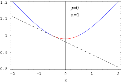
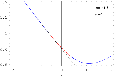
Figure 1: Plot of the asymptotic implied volatility $\Sigma_{\rm BS}(x;a,\varrho)$ in the log-normal discrete-time SABR model for parameters $a=1.0$ and $\varrho=0.0$ (left panel) and $\varrho=-0.5$ (right panel). The two branches in Theorem 16 are shown as the blue and red curves. The dashed line is the linear approximation (5.21).

Remark 17.

The result of Theorem 16 reveals the existence of three regions of log-strike separated by $x_{L}=-\frac{1}{2}\sigma_{0}^{2}T$ and $x_{R}=y_{R}\sigma_{0}^{2}T$. At the switch points we have

$$\sigma_{\rm BS}\left(x_{L},T\right)=\sigma_{0}\,,\quad\sigma_{\rm BS}\left(x_{R},T\right)=\sqrt{2y_{R}}\sigma_{0}\,.$$ (5.19)

This is illustrated in Figure 1 which shows the implied volatility function $\Sigma_{\rm BS}(y;a)$ for $a=1.0$ and correlation $\varrho=0$ (left) and $\varrho=-0.5$ (right). The three regions of Theorem 16 are shown with different colors. This is different from the SABR formula (6.15) which does not distinguish between these regions.

Remark 18.

The result of Theorem 16 is similar to the large maturity asymptotics for the Heston model derived by Forde and Jacquier [11]. However we note also a difference. In their result for the Heston model, the asymptotic implied volatility does not depend on $\sigma_{0}$, the initial condition for the volatility. This is because their rate function does not depend on $\sigma_{0}$. On the other hand, with our scaling $\sigma_{0}$ appears through the scaling variable $\rho$, which introduces dependence on $\sigma_{0}$ in the asymptotic implied volatility.

Remark 19.

For zero correlation $\varrho=0$, the implied volatility given by Theorem 16 is symmetric in log-strike (see the left panel in Fig. 1 for an illustration)

$$\sigma_{\rm BS}(-x,T)=\sigma_{\rm BS}(x,T)\,.$$ (5.20)

This follows from the symmetry relation (4.33) for the rate function in the zero correlation limit $\mathcal{I}_{X}(k,0)-\mathcal{I}_{X}(-k,0)=k$. This agrees with the well-known result of [44] that the implied volatility in an uncorrelated stochastic volatility model is a symmetric function of log-strike.

The leading quadratic term in the expansion of the rate function around its minimum at $y=-\frac{1}{2}$ gives a linear approximation for $\Sigma_{BS}(y;a)$ around $y=-\frac{1}{2}$

$$\Sigma_{BS}(y;a)=1-(1-\sqrt{c})\left(y+\frac{1}{2}\right)+O\left(\left(y+\frac{1}{2}\right)^{2}\right)\,,$$ (5.21)

with $c=\frac{1}{1+\frac{1}{6}a-\sqrt{\frac{a}{2}}\varrho}$. This linear approximation is shown as the dashed line in Fig. 1.

6 Limiting cases

We study in this section the limits of the asymptotic implied volatility of Theorem 16 in several regimes of short maturity $T\to 0$ and extreme strikes $|x|\to\infty$ at fixed maturity. The results are compared with existing results in the literature.

6.1 Short maturity limit

Consider the $T\to 0$ limit of the implied volatility. This limit is obtained by taking $a\to 0$ at fixed $\sqrt{a}y=\sqrt{2}\zeta$, with $\zeta=\frac{\omega}{\sigma_{0}}x$. Assuming that the limit exists, define

$$J(\zeta;\varrho):=\lim_{a\to 0,\sqrt{a}y=\sqrt{2}\zeta}\mathcal{J}_{X}(y;a,\varrho)\,.$$ (6.1)

Let us take this limit in the rate function $\mathcal{J}_{X}(y;a,\varrho)$, expressed as the extremal problem (4.22). This gives

$$J(\zeta;\varrho)=\inf_{u,v>0}\left\{\frac{1}{2}I(u,v)+\frac{2}{\varrho_{\perp}^{2}u}\left(\zeta-\varrho(v-1)\right)^{2}\right\}\,.$$ (6.2)

For $\zeta=0$ the minimizer is $u_{*}=1,v_{*}=1$; at this point the rate function vanishes $J(0;\varrho)=0$.

Proposition 20.

The solution of the extremal problem (6.2) for the rate function $J(\zeta;\varrho)$ has the expansion around $\zeta=0$

$$J(\zeta;\varrho)=2\zeta^{2}-2\varrho\zeta^{3}+\left(-\frac{2}{3}+\frac{5}{2}\varrho^{2}\right)\zeta^{4}+O(\zeta^{5})\,.$$ (6.3)

In the uncorrelated case $\varrho=0$ the extremal problem (6.2) can be solved exactly

$$J(\zeta;0)=2\log^{2}\left(\sqrt{\zeta^{2}+1}+|\zeta|\right)\,.$$ (6.4)

Proof.

The infimum condition in (6.2) can be expressed as the vanishing of the partial derivatives of the function of $(u,v)$ on the right hand side. This gives two equations for the extremal point $(u_{*},v_{*})$

$$u\partial_{u}I(u,v)=\frac{4}{\varrho^{2}_{\perp}u}\left(\zeta-\varrho(v-1)\right)^{2}\,,$$ (6.5)

$$v\partial_{v}I(u,v)=\frac{8\varrho}{\varrho^{2}_{\perp}u}v\left(\zeta-\varrho(v-1)\right)\,.$$

Introducing $\epsilon=\log u_{*},\eta=\log v_{*}$, the minimizers can be expanded in $\zeta$ as

$$\epsilon=a_{1}\zeta+a_{2}\zeta^{2}+O(\zeta^{3})\,,\quad\eta=b_{1}\zeta+b_{2}\zeta^{2}+O(\zeta^{3})\,.$$ (6.6)

Using the expansion for the rate function $I(u,v)$, the two equations in (6.5) can be expanded also in $\zeta$. Requiring the equality of the terms of each order in $\zeta$ gives successive equations for $a_{i},b_{j}$ which can be solved recursively. The first two coefficients are

$$a_{1}=b_{1}=\varrho\,,\quad a_{2}=\frac{2}{3}-\varrho^{2}\,,\quad b_{2}=\frac{1}{2}(1-2\varrho^{2})\,.$$ (6.7)

The coefficients $a_{1,2},b_{1,2}$ are sufficient to determine the expansion of the rate function $J(\zeta;\varrho)$ to order $O(\zeta^{2})$, with the result quoted in (6.3).

We give next the proof of (6.4) for the uncorrelated case. As $a\to 0$ at fixed $ay^{2}$ we have $|y|\to\infty$, such that we use the $y>y_{R}$ branch of the function $\Sigma_{\rm BS}(y;a)$ in Theorem 16. The rate function $\mathcal{J}_{X}(y;a,0)$ is given by Corollary 29. The equation for $\xi$ in this result becomes in this limit

$$\sinh^{2}\left(\frac{\xi}{2}\right)=\frac{1}{2}ay^{2}=\zeta^{2}\,,$$ (6.8)

which determines $\xi$ up to a sign as

$$\xi=\pm\log\left(1+2\zeta^{2}+2\sqrt{\zeta^{2}(1+\zeta^{2})}\right)=\pm 2\log\left(\sqrt{\zeta^{2}+1}+\sqrt{\zeta^{2}}\right)\,.$$ (6.9)

The rate function is

$$\lim_{a\to 0,ay^{2}=2\zeta^{2}}\mathcal{J}_{X}(y;a,0)=\frac{1}{2}\xi^{2}=\xi\tanh(\xi/2)+2\zeta^{2}\frac{\xi}{\sinh\xi}=2\log^{2}\left(\sqrt{\zeta^{2}+1}+\sqrt{\zeta^{2}}\right)\,.$$ (6.10)

∎

Remark 21.

The expansion (6.3) agrees with the first three terms in the Taylor expansion of the function

$$\tilde{J}(\zeta,\varrho):=2\log^{2}\frac{\sqrt{1+2\varrho\zeta+\zeta^{2}}+\zeta+\varrho}{1+\varrho}\,.$$ (6.11)

Numerical testing shows that the rate function $J(\zeta;\varrho)$ is reproduced to very good precision by this function; however we could not prove their equality analytically, except for the uncorrelated case $\varrho=0$, when (6.11) reduces to (6.4).

The asymptotic implied volatility in the small-maturity limit can be expressed in terms of the rate function $J(\zeta;\varrho)$ given by the limit (6.1).

Proposition 22.

Assume that the limit (6.1) exists and is given by the rate function $J(\zeta;\varrho)$. Then the implied volatility in the $T\to 0$ limit of the SABR model with correlation $\varrho$ and $\omega\to 0,\sigma_{0}\to\infty$ at fixed $\sigma_{0}\omega$ is

$$\lim_{\sigma_{0}\to\infty}\frac{1}{\sigma_{0}}\sigma_{\rm BS}(x,T)=\frac{\sqrt{2}\zeta}{\sqrt{J(\zeta;\varrho)}},\qquad\text{with $\zeta=\frac{\omega}{\sigma_{0}}x$}.$$ (6.12)

Proof.

Start with the result for $\Sigma_{\rm BS}(y;a)$ from Theorem 15

$$\Sigma_{\rm BS}(y;a)=\left|\sqrt{\frac{1}{a}\mathcal{J}_{X}(y;a,\varrho)-2y}-\sqrt{\frac{1}{a}\mathcal{J}_{X}(y;a,\varrho)}\right|\,,\quad y>y_{R}\mbox{ and }y<-\frac{1}{2},$$ (6.13)

We choose the $y>y_{R},y<-\frac{1}{2}$ branch since as $a\to 0$, the product $\sqrt{a}y$ can be constant only if $y\to\infty$. Expanding this result for $a\to 0$ we get

$$\Sigma_{\rm BS}(y;a)=\sqrt{\frac{1}{a}\mathcal{J}_{X}(y;a,\varrho)}\left(1-\sqrt{1-\frac{2ya}{\mathcal{J}_{X}(y;a,\varrho)}}\right)=\frac{\sqrt{a}y}{\sqrt{\mathcal{J}_{X}(y;a,\varrho)}}+O(a^{3/2}y^{2})\,.$$

Taking the $a\to 0$ limit at fixed $\sqrt{a}y=\sqrt{2}\zeta$ gives

$$\lim_{a\to 0}\Sigma_{\rm BS}(y;a)=\frac{\sqrt{2}\zeta}{\sqrt{J(\zeta;\varrho)}}\,,$$ (6.14)

where $J(\zeta;\varrho)$ is given by the limit (6.1).

∎

Substituting the expansion (6.3) into (6.12) reproduces the first three terms in the expansion of the celebrated analytical formula for the implied volatility in the SABR model in the short maturity asymptotic limit [23]

$$\sigma_{\rm BS}(x,T)=\sigma_{0}\frac{\zeta}{D(\zeta;\varrho)}\left(1+\left(\frac{1}{4}\varrho\omega_{0}\sigma_{0}+\frac{1}{24}(2-3\varrho^{2})\omega^{2}\right)T+O(T^{2})\right)\,.$$ (6.15)

with

$$D(\zeta;\varrho):=\log\frac{\sqrt{1+2\zeta\varrho+\zeta^{2}}+\zeta+\varrho}{1+\varrho}\,,$$ (6.16)

and the $O(T)$ terms holds only at the at-the-money (ATM) point $x=0$ [38]. Assuming $J(\zeta;\varrho)=\tilde{J}(\zeta;\varrho)$ reproduces the first factor in (6.15).

The result (6.15) is the leading order term in a short maturity expansion, and the next two terms in this expansion have been subsequently derived by Henry-Labordere [24] and Paulot [37]. The ATM limit of this result is $\sigma_{\rm BS}(0,0)=\sigma_{0}$.

In Figure 2 we compare the asymptotic result (colored curves) with the SABR formula (6.15) (dashed black curve), for the model parameters $\sigma_{0}=0.2,\omega=1,\varrho=-0.75$, for several maturities $T=0.25-5.0$. For sufficiently small maturity $T$, corresponding to small values of the $a=2(\omega^{2}T)(\sigma_{0}^{2}T)$ parameter, the asymptotic result agrees very well with the short maturity limit (6.15).

6.2 Short maturity expansion for the ATM implied volatility

We study here the $T\to 0$ expansion of the asymptotic implied volatility at the ATM point.

Proposition 23.

(i) The first few terms in the expansion of the ATM asymptotic implied volatility $\sigma_{\rm BS}(0,T)$ in powers of $a=2\sigma_{0}^{2}\omega^{2}T^{2}$ are

$$\frac{1}{\sigma_{0}}\sigma_{\rm BS}(0,T)=\Sigma_{\rm BS}(0;a) =1+\frac{\varrho}{4\sqrt{2}}\sqrt{a}+\left(-\frac{1}{48}+\frac{1}{16}\varrho^{2}\right)a+O(a^{3/2})$$ (6.17)

$$=1+\frac{1}{4}\varrho\omega\sigma_{0}T-\frac{1}{24}(1-3\varrho^{2})\sigma_{0}^{2}\omega^{2}T^{2}+O(T^{3})\,.$$

(ii) In the uncorrelated limit $\varrho=0$ the expansion contains only integer powers of $a$

$$\Sigma_{\rm BS}(0;a)=1-\frac{1}{48}a+\frac{43}{23040}a^{2}-\frac{1907}{7741440}a^{3}-\frac{51083}{7431782400}a^{4}+O(a^{5})\,.$$ (6.18)

which means that the implied volatility contains only even powers of $T$

$$\frac{\sigma_{\rm BS}(0,T)}{\sigma_{0}}=1-\frac{1}{24}\sigma_{0}^{2}\omega^{2}T^{2}+\frac{43}{5760}\sigma_{0}^{4}\omega^{4}T^{4}+O(T^{6})\,.$$ (6.19)

Proof.

(i) Taking $x=0$ in Theorem 16 gives the ATM asymptotic implied volatility $\Sigma_{\rm BS}(0;a)=2\sqrt{\frac{1}{a}\mathcal{J}_{X}(0;a,\varrho)}$. The rate function $\mathcal{J}_{X}(0;a,\varrho)$ is given by the extremal problem (4.22). This can be expanded as $a\to 0$ by expanding the minimizers in this problem around $u=v=1$. Denoting the minimizers $u_{*},v_{*}$, this expansion reads

$$\epsilon=\log u_{*}=a_{1}\sqrt{a}+a_{2}a+O(a^{3/2})\,,\quad\eta=\log v_{*}=b_{1}\sqrt{a}+b_{2}a+O(a^{3/2})\,.$$ (6.20)

Using the expansion (5) for the rate function $I(u,v)$, the coefficients $a_{i},b_{i}$ can be determined recursively. Substituting into (4.22) gives the expansion of the rate function

$$\mathcal{J}_{X}(0;a,\varrho)=\frac{1}{4}a+\frac{\varrho}{8\sqrt{2}}a^{3/2}+\frac{1}{384}(-4+15\varrho^{2})a^{2}+O(a^{5/2})\,.$$ (6.21)

Finally, substituting into $\Sigma_{\rm BS}(0;a)=2\sqrt{\frac{1}{a}\mathcal{J}_{X}(0;a,\varrho)}$ gives the expansion (6.17).

(ii) The rate function $\mathcal{J}_{X}(y;a,0)$ is given in closed form by Eq. (A.10)

$$\mathcal{J}_{X}(0;a,0)=2\lambda(\tan\lambda-\lambda)+a\frac{\sin 2\lambda}{2\lambda}=2\lambda(2\tan\lambda-\lambda)\,,$$ (6.22)

where $\lambda$ is the solution of the equation

$$\frac{\lambda^{2}}{\cos^{2}\lambda}=\frac{a}{8}\,.$$ (6.23)

The last equality in (6.22) follows by substituting $a$ from (6.23).

Expanding the solution for $\lambda$ in powers of $\sqrt{a}$ and substituting into (6.22) gives

$$\mathcal{J}_{X}(0;a,0)=\frac{1}{4}a-\frac{1}{96}a^{2}+\frac{1}{960}a^{3}-\frac{23}{161280}a^{4}+O(a^{5})\,.$$ (6.24)

This can be translated as before into an expansion for the asymptotic ATM implied volatility.

∎

We can compare these expansions with the results in the literature. The $O(T)$ term in (6.17) coincides with the first $O(T)$ term in the short maturity expansion of the implied volatility (6.15). This expansion has been extended to $O(T^{2})$ by Paulot [38], where the $O(T^{2})$ term was evaluated partially numerically. A closed form result for the ATM implied volatility expansion in the log-normal ($\gamma=1$) SABR model to $O(T^{2})$ has been communicated to us by Alan Lewis [34]

$$\frac{1}{\sigma_{0}}\sigma_{\rm BS}(0,T)=1+\frac{1}{24}\sigma_{0}\omega T\left[6\varrho+\frac{\omega}{\sigma_{0}}(2-3\varrho^{2})\right]$$ (6.25)

$$+\frac{1}{1920}\omega^{2}\sigma_{0}^{2}T^{2}\left[(-80+240\varrho^{2})+\frac{\omega}{\sigma_{0}}\varrho(240-180\varrho^{2})+\frac{\omega^{2}}{\sigma_{0}^{2}}(-12+60\varrho^{2}-45\varrho^{4})\right]+O(T^{3})\,.$$

The short maturity expansion of the implied volatility in a wide class of stochastic volatility models called MAP-like (Markov Additive Processes) which include $\gamma=1$ SABR, is known ([33] page 505) to admit a double series expansion in $(x=\log(K/S_{0}),T)$.

Recalling that the asymptotic limit considered in our paper corresponds to $\omega^{2}T\ll 1,\sigma_{0}\omega=O(1)$, it is easy to see that (6.17) is reproduced by taking this limit in (6.25).

The existence of the limit $\omega^{2}T\to 0,\sigma_{0}\omega_{0}=O(1)$ constrains the form of the higher order terms in the ATM implied volatility

$$\frac{\sigma_{BS}(0,T)}{\sigma_{0}}=1+\left(c_{1}^{(1)}\omega\sigma_{0}+c_{1}^{(0)}\omega^{2}\right)T+\sum_{k=2}^{\infty}\sigma_{k}(\omega,\sigma_{0},\varrho)T^{k}\,.$$ (6.26)

Assume that $\sigma_{k}(\omega,\sigma_{0},\varrho)T^{k}$ is a polynomial in $(\omega\sqrt{T}),(\sigma_{0}\sqrt{T})$ of order $2k$, this must have the form

$$\sigma_{k}(\omega,\sigma_{0},\varrho)=\sum_{j=0}^{k}c_{k}^{(j)}(\varrho)\omega^{2k-j}\sigma_{0}^{j}\,.$$ (6.27)

For example, a $O(T^{2})$ term of the form $\omega\sigma_{0}^{3}T^{2}$ is not allowed, as it diverges in the limit considered.

In the limit considered, only the terms proportional to $c_{k}^{(k)}$ contribute. The expansion of Proposition 23 determines these coefficients. For example we get $c_{4}^{(4)}(\varrho)=\frac{1}{5760}(43-375\varrho^{2}+315\varrho^{4})$ for the coefficient of $(\omega\sigma_{0}T)^{4}$, which has been confirmed by explicit computation [34].

6.3 Extreme strikes asymptotics

We study here asymptotics in the extreme strikes region $|x|\to\infty$ for the uncorrelated case $\varrho=0$. Since the implied volatility is symmetric in $x$ for this case, see Remark 19, it will be sufficient to study asymptotics for large strike $x\to\infty$.

Proposition 24.

In the large log-strike region $x\to\infty$, the asymptotic volatility (5.17) in the uncorrelated log-normal SABR model $\varrho=0$ has the expansion

$$\Sigma_{\rm BS}(x;a,0) =\sqrt{2x}-\frac{1}{\sqrt{2a}}\log(2x)-\frac{1}{2a}\log(2\log(2x))+\frac{1}{\sqrt{2a}}$$ (6.28)

$$\quad+\frac{1}{4a\sqrt{2x}}\log^{2}(2x)+\frac{1}{2a\sqrt{2x}}\log(2x)\log(2\log(2x))+O\left(\frac{\log(2\log(2x))}{\log(2x)}\right)\,.$$

Proof.

We use the result of Proposition 31 for the large argument limit of the rate function to obtain the asymptotics of $\Sigma_{\rm BS}(x;a,0)$ for $x\to\infty$

$$\Sigma_{\rm BS}(x;a,0) =\Sigma_{\rm BS}(-x;a,0)=\sqrt{\frac{1}{a}J_{X}(x;a,0)}-\sqrt{-2x+\frac{1}{a}J_{X}(x;a,0)}$$ (6.29)

$$=\sqrt{2x}\left(\sqrt{1+r(x,a)}-\sqrt{r(x,a)}\right)$$

$$=\sqrt{2x}\left(1-\sqrt{r(x,a)}+\frac{1}{2}r(x,a)+O(r^{2}(x,a))\right)\,,$$

where

$$r(x,a)=\frac{1}{4ax}\log^{2}(2x)+\frac{1}{2ax}\log(2x)\log(2\log(2x))-\frac{1}{2ax}\log(2x)+O\left(\frac{\log\log x}{2ax}\right)\,.$$ (6.30)

Expanding the result gives (6.28). ∎

Corollary 25.

The large strike asymptotics of the implied variance for $x\to\infty$ at fixed $T$ is given by

$$\sigma_{\rm BS}^{2}(x,T)T=\sigma_{0}^{2}\Sigma_{\rm BS}^{2}\left(\frac{x}{\sigma_{0}^{2}T},a,0\right)T=\frac{2x}{\left(\sqrt{1+r\left(\frac{x}{\sigma_{0}^{2}T},a\right)}+\sqrt{r\left(\frac{x}{\sigma_{0}^{2}T},a\right)}\right)^{2}}\,,$$ (6.31)

with $a=2(\omega^{2}T)(\sigma_{0}^{2}T)$ and

$$r\left(\frac{x}{\sigma_{0}^{2}T},a\right)=\frac{1}{4\omega^{2}Tx}\left\{\frac{1}{2}\log^{2}\left(\frac{2x}{\sigma_{0}^{2}T}\right)+\log\left(\frac{2x}{\sigma_{0}^{2}T}\right)\log\left(2\log\left(\frac{2x}{\sigma_{0}^{2}T}\right)\right)-\log\left(\frac{2x}{\sigma_{0}^{2}T}\right)\right\}\,.$$ (6.32)

Using the expansion $(\sqrt{1+r}+\sqrt{r})^{-2}=1-2\sqrt{r}+2r+O(r^{3/2})$ we get, keeping only the $O(\sqrt{r})$ term,

$$\sigma_{\rm BS}^{2}(x,T)T =2x\left(1-\frac{1}{\sqrt{2\omega^{2}Tx}}\sqrt{L^{2}+2L\log(2L)-2L}+\cdots\right)$$ (6.33)

$$=2x-\frac{\sqrt{2x}}{\sqrt{\omega^{2}T}}\sqrt{L^{2}+2L\log(2L)-2L}+\cdots\,,$$

where we denoted $L=\log\left(\frac{2x}{\sigma_{0}^{2}T}\right)$.

The leading term in (6.33) agrees with the result expected from Lee’s moment formula. Recall that under the Log-Euler-log-Euler scheme, all moments $\mathbb{E}[(S_{n})^{1+\varepsilon}]$ with $\varepsilon>0$ are infinite [41]. The Lee moment formula [28] predicts that the large strike asymptotics of the implied variance is $\lim_{x\to\infty}\sigma_{\rm BS}^{2}(x,T)T=2x$.

The short maturity SABR formula (6.15) gives an implied volatility which grows faster than the behavior expected from the Lee’s moment formula. Therefore its applicability is limited to a region of log-strikes sufficiently close to the at-the-money region.

The result (6.33) agrees with the subleading correction derived by Gulisashvili and Stein in the uncorrelated Hull-White model [19]. In Theorem 3.1 and Corollary 3.1 of this paper, the following asymptotic result is proved in this model (assuming $S_{0}=1$)

$$\sigma_{\rm BS}^{2}(K,T)T=2\log K-\frac{1}{\omega\sqrt{T}}\sqrt{2\log K}(\log\log K+\log\log\log K)+\cdots\,.$$ (6.34)

The leading correction term to the Lee’s moment formula $\sim\log\log K$ agrees with (6.33).

7 Numerical benchmarks

We compare in this section numerical benchmarks for implied volatility in the $\gamma=1$ SABR model, with the asymptotic results of this paper.

Table 2: Scenarios for the numerical testing, from Table 8.6 in [33]. The model parameters are $\sigma_{0}=0.2,\omega=1.0,\varrho=-0.75$. The table shows the parameter $a=2(\omega^{2}T)(\sigma_{0}^{2}T)$ of the asymptotic expansion, the point $(u_{m},v_{m})$ determined by Corollary 9 and the right switch point $y_{R}$ given by (4.29).

$T$	$a$	$\sigma_{0}^{2}T$	$(u_{m},v_{m})$	$y_{R}$
0.25	0.005	0.01	(0.9636, 0.9638)	0.4821
1.0	0.08	0.04	(0.8664, 0.8692)	0.4362
2.0	0.32	0.08	(0.7589, 0.7676)	0.3882
5.0	2.0	0.20	(0.5360, 0.5636)	0.2938

The benchmark option prices are taken from Table 8.6 in [33]. They were obtained using the transform method of [31, 33] with the model parameters $\sigma_{0}=0.2,\omega=1.0,\varrho=-0.75$ and several option maturities $T=0.25,1,2,5$.

The asymptotic result $\sigma_{\rm BS}(x,T)/\sigma_{0}$ of Theorem 16 (blue/red curve) is compared against the benchmark values in Figure 2 (black dots). The three regions of Theorem 16 are shown in different colors (red for the central region $-\frac{1}{2}\sigma_{0}^{2}T\leq x\leq y_{R}\sigma_{0}^{2}T$). The figures show also the leading order $O(T^{0})$ short-maturity asymptotics in the SABR model (6.15) as the dashed black curve.

From these results we note the following observations:

(i) For short maturities the agreement of the asymptotic result with the SABR asymptotic formula (6.15), and with the numerical benchmark results is very good. The central region of log-strikes of Theorem 16 is very small, and it expands as the maturity increases.

(ii) At larger maturities the short-maturity approximation (6.15) overestimates the actual implied volatility. While the asymptotic result reproduces the decreasing trend of the numerical result, it is an overestimate for longer maturities.

As explained in the previous section, the asymptotic result holds in the limit $\sigma_{0}/\omega\gg 1$. The numerical benchmarks considered have $\sigma_{0}/\omega=0.2$ which is not particularly large. The agreement is expected to become better if this ratio is large, corresponding to a small vol-of-vol scenario. This is confirmed by the results in Table 3 where the asymptotic result for the ATM implied volatility is compared with numerical benchmarks for a scenario with $\sigma_{0}=1.0,\omega=0.1$. The agreement improves in the latter case, as expected.

(iii) From Table 3 one observes that in the uncorrelated case $\varrho=0$, the actual ATM implied volatility has a non-monotonic dependence on maturity: starts at $\sigma_{0}$ as $T\to 0$, first increases with maturity, and then decreases as $T\to\infty$. On the other hand, the asymptotic result has a monotonously decreasing trend.

The discrepancy between the two results at short maturity can be traced back to the absence of a $O(T)$ term in the asymptotic expansion for the uncorrelated case, which is responsible for the increasing trend of the numerical results for small maturity. Using the full $O(T^{2})$ expansion for the ATM implied volatility (6.25), which includes this term, reproduces well the benchmark results, as shown in Table 3.

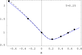
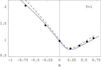
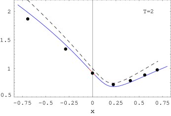
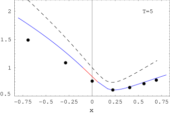
Figure 2: Plots of the asymptotic implied volatilities $\sigma_{\rm BS}(x,T)/\sigma_{0}$ vs $x=\log(K/S_{0})$ (colored curves) for the scenarios in Table 2, taken from Table 8.6 of [33]. The black dots show the benchmark values from [33], and the dashed black curve shows the short maturity SABR implied volatility. The different regions in Theorem 16 are shown in different colors (blue/red).

Table 3: Benchmark numerical values computed using the transform method (AL) [33] and the second order short maturity expansion $O(T^{2})$ from (6.25) for maturities $T=0.25,1,2,5,50$, comparing with the asymptotic results from Theorem 16. The model parameters are $(\sigma_{0},\omega)=(0.2,1.0),(1.0,0.1)$ and $\varrho=0$.

	$\sigma_{0}=0.2,\omega=1.0$			$\sigma_{0}=1.0,\omega=0.1$
$T$	AL	$O(T^{2})$ expansion	asymptotic	AL	$O(T^{2})$ expansion	asymptotic
0.25	0.20407	0.204068	0.19998	1.00018	1.00018	0.99997
1.0	0.21460	0.215083	0.19967	1.00041	1.00042	0.99958
2.0	0.22123	0.227	0.19870	0.999974	0.999998	0.99835
5.0	0.20451	0.24375	0.19286	0.993662	0.993734	0.99002
50.0	0.07822	-2.925	0.11275	0.719669	-0.0015625	0.72071

Appendix A The zero correlation case

The rate function $\mathcal{I}_{X}(x;\varrho)$ simplifies in the uncorrelated limit $\varrho=0$, and can be expressed in closed form. This result can be used to derive the asymptotics of the rate function in various limits of small/large arguments. We give in this Appendix these results and their proofs.

A.1 The rate function $J_{\rm BS}(x)$

The rate function appearing in the LDP for $\mathbb{P}(\frac{1}{n}V_{n}\in\cdot)$ can be extracted from Proposition 6 in [42]. A simpler form is given in Corollary 13 of the same paper, in terms of the function $J_{\rm BS}(x)$. We reproduce here this result for ease of reference.

Proposition 26.

Define $A_{n}:=\sum_{i=0}^{n-1}e^{sZ_{i}+(m-\frac{1}{2}s^{2})t_{i}}$, with $Z_{i}$ a standard Brownian motion sampled on uniformly distributed times $t_{i}=\tau i$. Consider the $n\to\infty$ limit at fixed $b=\frac{1}{2}s^{2}\tau n^{2}$ and $r=m\tau n$. In this limit $\mathbb{P}(\frac{1}{n}A_{n}\in\cdot)$ satisfies a LDP with rate function $I_{\rm BS}(\cdot)=\frac{1}{2b}J_{\rm BS}(\cdot)$. For $r=0$, the rate function $\mathcal{J}_{\rm BS}(x)$ is given by

$$\mathcal{J}_{\rm BS}(x)=\begin{cases}\frac{1}{2}\xi^{2}-\xi\tanh(\xi/2)&\text{for $x\geq 1$},\\ 2\lambda(\tan\lambda-\lambda)&\text{for $0<x\leq 1$},\\ 0&\text{for $x=1$},\end{cases}$$ (A.1)

where $\xi>0$ is the unique solution of the equation

$$\frac{1}{\xi}\sinh\xi=x\,,$$ (A.2)

and $\lambda\in(0,\frac{\pi}{2})$ is the unique solution of the equation

$$\frac{1}{2\lambda}\sin(2\lambda)=x\,.$$ (A.3)

The sum $V_{n}=\sum_{i=0}^{n-1}\sigma_{i}^{2}\tau$ is obtained by identifying $\frac{V_{n}}{\sigma_{0}^{2}\tau}\to A_{n}$ with the substitutions $s\to 2\omega,m\to\omega^{2}$. In the $n\to\infty$ limit at fixed $b=\frac{1}{2}s^{2}\tau n^{2}=2\omega^{2}\tau n^{2}$, it is clear that $r=mn\tau=\omega n\tau\to 0$. This justifies the $r=0$ limit used in (A.1).

We will require also the derivative of the rate function $\mathcal{J}_{\rm BS}(x)$. This can be obtained in closed form and is given by the following result.

Corollary 27.

The derivative of the rate function $\mathcal{J}_{\rm BS}(x)$ is given by

$$\mathcal{J}^{\prime}_{\rm BS}(x)=\begin{cases}\frac{1}{2}\frac{\xi^{2}}{\cosh^{2}(\xi/2)}&\text{for $x>1$},\\ -2\frac{\lambda^{2}}{\cos^{2}\lambda}&\text{for $0<x<1$},\end{cases}$$ (A.4)

where $\xi$ is the solution of the equation (A.2) and $\lambda$ is the solution of the equation (A.3).

A.2 Closed form result for the rate function $\mathcal{I}_{X}(x;\varrho=0)$

The rate function $\mathcal{I}_{X}(x;\varrho)$ giving the large deviations for $\mathbb{P}(\frac{1}{n}\log S_{n}\in\cdot)$ is given by the solution of the extremal problem in Proposition 10 in the main text. In the zero correlation limit $\varrho=0$ this extremal problem simplifies to a one-dimensional extremal problem. Using the one dimensional projection relation $\inf_{v}I(u,v)=2\mathcal{J}_{\rm BS}(u)$, the extremal problem (4.22) simplifies as

$$\mathcal{J}_{X}(y;a,0) =\inf_{u,v}\left\{\frac{1}{2}I(u,v)+\frac{a}{u}\left(y+\frac{1}{2}u\right)^{2}\right\}$$ (A.5)

$$=\inf_{u}\left\{\mathcal{J}_{\rm BS}(u)+\frac{a}{u}\left(y+\frac{1}{2}u\right)^{2}\right\}=\mathcal{J}_{\rm BS}(u_{*})+\frac{a}{u_{*}}\left(y+\frac{1}{2}u_{*}\right)^{2}\,,$$

where we denoted in the last line the optimal value of $u$ in the extremal problem as $u_{*}(y)$.

Lemma 28.

The extremal value $u_{*}(y)$ has the following properties:

(i) $u_{*}(y)>1$ for $|y|>\frac{1}{2}$;

(ii) $0<u_{*}(y)<1$ for $|y|<\frac{1}{2}$.

Proof.

The optimal value $u_{*}(y)$ is given by the solution of the equation

$$\mathcal{J}_{\rm BS}^{\prime}(u)+\frac{a}{u^{2}}\left(\frac{1}{4}u^{2}-y^{2}\right)=0\,.$$ (A.6)

This equation can be written equivalently as

$$\mathcal{J}_{\rm BS}^{\prime}(u)=a\left(\frac{y^{2}}{u^{2}}-\frac{1}{4}\right).$$ (A.7)

The function on the right side is decreasing in $u$ and is positive at $y=1$ for $|y|>\frac{1}{2}$, and negative for $|y|<\frac{1}{2}$. The function on the left side is increasing and vanishes at $y=1$. This implies that the two sides will become equal at a point $u_{*}(y)$ which is larger than $1$ in the first case, and lower than $1$ in the second case. This proves the claim. ∎

We give next a closed form result for the rate function, which is useful for numerical evaluations and deriving asymptotic expansions.

Corollary 29.

In the zero correlation limit $\varrho=0$, the rate function $\mathcal{J}_{X}(y;a,0)$ has the following explicit form.

Case 1. $|y|>\frac{1}{2}$.

$$\mathcal{J}_{X}(y;a,0)=\frac{1}{2}\xi^{2}-\xi\tanh(\xi/2)+a\frac{\xi}{\sinh\xi}\left(y+\frac{1}{2\xi}\sinh\xi\right)^{2}\,,$$ (A.8)

where $\xi\in(0,\infty)$ satisfies the equation

$$\frac{1}{4a}\frac{\xi^{2}}{\cosh^{2}(\xi/2)}+\frac{1}{8}-\frac{1}{2}y^{2}\frac{\xi^{2}}{\sinh^{2}\xi}=0\,.$$ (A.9)

Case 2. $|y|<\frac{1}{2}$.

$$\mathcal{J}_{X}(y;a,0)=2\lambda(\tan\lambda-\lambda)+a\frac{2\lambda}{\sin 2\lambda}\left(y+\frac{1}{2}\frac{\sin 2\lambda}{2\lambda}\right)^{2}\,,$$ (A.10)

where $\lambda\in(0,\pi/2)$ satisfies the equation

$$-\frac{1}{a}\frac{\lambda^{2}}{\cos^{2}\lambda}+\frac{1}{8}-\frac{1}{2}y^{2}\frac{(2\lambda)^{2}}{\sin^{2}(2\lambda)}=0\,.$$ (A.11)

Case 3. $|y|=\frac{1}{2}$.

$$\mathcal{J}_{X}\left(-\frac{1}{2};a,0\right)=0,\qquad\mathcal{J}_{X}\left(\frac{1}{2};a,0\right)=a.$$ (A.12)

Proof.

Case 1. $|y|>\frac{1}{2}$. For this case $u_{*}>1$ so we use the corresponding branch of $\mathcal{J}_{\rm BS}(u)$, with $u_{*}=\frac{\sinh\xi}{\xi}$. The value of $\xi$ is determined by expressing (A.6) as an equation for $\xi$. This reproduces (A.9). The rate function is obtained by substituting $u_{*}$ into (A.5). This reproduces (A.8).

Case 2. $|y|<\frac{1}{2}$. For this case $0<u_{*}<1$ and we use the second branch of $\mathcal{J}_{\rm BS}(u)$, with $u_{*}=\frac{\sin(2\lambda)}{(2\lambda)}$. The equation for $\lambda$ is obtained by substituting the expression for $u_{*}$ into (A.6). This reproduces (A.11). Proceeding in a similar way we get the rate function by substituting $u_{*}$ into (A.5), which reproduces (A.10). ∎

Proposition 30.

The rate function in the uncorrelated case satisfies the symmetry relation

$$J_{X}(y;a,0)-J_{X}(-y;a,0)=2ay\,.$$ (A.13)

Proof.

This follows by noting that the optimizer $u_{*}(y)$, the solution of the equation (A.6) is a symmetric function in $y$. If $u_{*}(y)$ is a solution of this equation for a certain $y$, it will be also a solution for $-y$. Thus we have

$$J_{X}(y;a,0)-J_{X}(-y;a,0)=\frac{a}{u_{*}}\left(y+\frac{1}{2}u_{*}\right)^{2}-\frac{a}{u_{*}}\left(-y+\frac{1}{2}u_{*}\right)^{2}=2ay\,.$$ (A.14)

∎

A.3 Asymptotic expansion for $\mathcal{J}_{X}(x;a,0)$

We derive here the asymptotic expansion for the rate function $\mathcal{J}_{X}(x;a,0)$ for very large argument $|x|\to\infty$.

Proposition 31.

As $x\to\infty$ the rate function $\mathcal{J}_{X}(x;a,0)$ has the expansion

$$\mathcal{J}_{X}(x;a,0)=2ax+\frac{1}{2}\log^{2}(2x)+\log(2x)\log(2\log(2x))-\log(2x)+O(\log\log x).$$ (A.15)

Proof.

We use the explicit form for the rate function $\mathcal{J}_{X}(x;a,0)$ given in Corollary 29. This has two branches, for $|x|>\frac{1}{2}$ and $|x|<\frac{1}{2}$. We are interested in $x\gg 1$ so we give below only the result for $x>\frac{1}{2}$ for ease of reference.

$$\mathcal{J}_{X}(x;a,0)=\frac{1}{2}\xi^{2}-\xi\tanh(\xi/2)+a\frac{\xi}{\sinh\xi}\left(x+\frac{1}{2\xi}\sinh\xi\right)^{2}\,,$$ (A.16)

where $\xi$ is the solution of the equation

$$\frac{1}{4a}\frac{\xi^{2}}{\cosh^{2}(\xi/2)}+\frac{1}{8}-\frac{1}{2}x^{2}\frac{\xi^{2}}{\sinh^{2}\xi}=0\,.$$ (A.17)

The first two terms in (A.16) correspond to $\mathcal{J}_{\rm BS}(y)$ in (4.21). The asymptotics of $\mathcal{J}_{\rm BS}(y)$ for $y\to\infty$ was obtained in Proposition 13 in [40]. We will follow a similar approach to obtain the asymptotics of $\mathcal{J}_{X}(x;a,0)$ for $x\to\infty$.

The strategy will be to invert the equation (A.17) for $x\gg 1$ and use the resulting expansion for $\xi(x)$ into (A.16). First we write the equation (A.17) for $\xi$ as

$$\frac{1}{2a}\frac{\sinh^{2}\xi}{\cosh^{2}(\xi/2)}+\frac{1}{4}\frac{\sinh^{2}\xi}{\xi^{2}}=x^{2}\,,$$ (A.18)

$$\frac{2}{a}\sinh^{2}(\xi/2)+\frac{1}{4}\frac{\sinh^{2}\xi}{\xi^{2}}=x^{2}\,,$$ (A.19)

$$\sinh^{2}(\xi/2)\left(\frac{2}{a}+\frac{\cosh^{2}\xi}{\xi^{2}}\right)=x^{2}\,.$$ (A.20)

We solve this equation for $\xi$ as $x\to\infty$ using asymptotic inversion, see for example Sec.1.5 in [36]. We first write the equation (A.20) for $\xi$ as

$$e^{\xi}\left(1-e^{-\xi}\right)^{2}\left(\frac{1}{2a}+\frac{1}{16\xi^{2}}e^{\xi}\left(1+e^{-\xi}\right)^{2}\right)=x^{2}\,.$$ (A.21)

Take logs of both sides

$$\xi+2\log(1-e^{-\xi})+\xi+2\log(1+e^{-\xi})-2\log(4\xi)+\log\left(1+\frac{8\xi^{2}e^{-\xi}}{a(1+e^{-\xi})^{2}}\right)=\log x^{2}\,,$$

or equivalently

$$2\xi=\log x^{2}-2\log\left(1-e^{-2\xi}\right)+2\log(4\xi)-\log\left(1+\frac{8\xi^{2}e^{-\xi}}{a(1+e^{-\xi})^{2}}\right)\,.$$

As $x\to\infty$, this is approximated as $2\xi=\log x^{2}+O(\log\xi)$. This estimate can be improved by iteration, starting with this first order approximation and solving for $\xi^{(i+1)}$ by inserting the previous iteration on the right-hand side. The first two iterations are

$$2\xi^{(1)}=\log x^{2}+O(\log\log x^{2})\,,$$ (A.22)

$$2\xi^{(2)}=\log x^{2}+2\log(2\log x^{2})+O\left(\frac{\log\log x^{2}}{\log x^{2}}\right)\,.$$ (A.23)

To this order, the dependence on $a$ is of higher order. This means that we can approximate the equation (A.20) for $\xi$ with $\frac{\sinh\xi}{\xi}=2x$ (by neglecting the $a$ term) and we can read off the solution from the Prop. 13 in [40] by replacing $K/S_{0}\to 2x$.

Thus we get the expansion of the first 2 terms in the rate function (A.16) (given by $\mathcal{J}_{\rm BS}(y_{*})$) from Prop. 13 in [40]

$$\mathcal{J}_{\rm BS}(y_{*}) =\frac{1}{2}\log^{2}(2x)+\log(2x)\log(2\log(2x))-\log(2x)$$ (A.24)

$$\qquad+3\log^{2}(2\log(2x))-2\log(2\log(2x))+O(\log^{-1}(2x))\,.$$

The second term in (A.16) is

$$a\frac{\xi}{\sinh\xi}\left(x+\frac{1}{2\xi}\sinh\xi\right)^{2}=\frac{a}{2x}\left(x+\frac{1}{2}2x\right)^{2}=2ax\,.$$ (A.25)

Adding them gives

$$\mathcal{J}_{X}(x;a,0)=2ax+\frac{1}{2}\log^{2}(2x)+\log(2x)\log(2\log(2x))-\log(2x)+O(\log\log x)\,.$$

This completes the proof of Eq. (A.15). ∎

References

- [1] Antonov, A., M. Konikov and M. Spector, Modern SABR analytics, Springer, New York 2019
- [2] Antonov, A., M. Konikov and M. Spector, SABR spreads its wings. Risk, August 2013.
- [3] Berestycki, H., J. Busca and I. Florent, Computing the implied volatility in stochastic volatility models, Commun. Pure Appl. Math. 57, 1352-1373 (2004).
- [4] Bernard, C., Z. Cui and D. McLeish, On the martingale property in stochastic volatility models based on time-homogeneous diffusions, Math. Finance 27(1), 194-223 (2017)
- [5] Cai, N., Y. Song and N. Chen, Exact simulation of the SABR model, Operations Research 65(4): 931-951 (2017).
- [6] Constantinescu, R., N. Costanzino, A.L. Mazzucato and V. Nistor, Approximate solutions to second order parabolic equations: I. Analytical estimates, J. Math. Phys. 51, 103502 (2010).
- [7] Dembo, A. and O. Zeitouni. Large Deviations Techniques and Applications. 2nd Edition, Springer, New York, 1998.
- [8] Deuschel, J. D., P.K. Friz, A. Jacquier and S. Violante, Marginal density expansions for diffusions and stochastic volatility, part I: Theoretical Foundations, Comm. Pure Appl. Math. 67, 40-82 (2014).
- [9] Donsker, M.D. and S. R. S. Varadhan. (1975). Asymptotic evaluation of certain Markov process expectations for large time. I. Comm. Pure Appl. Math. 28, 1-47.
- [10] Forde, M. and A. Jacquier, Small-time asymptotics for implied volatility under the Heston model, Int. J. Theor. Appl. Finance 12, 861-876 (2009).
- [11] Forde, M. and A. Jacquier, The large-maturity smile for the Heston model, Finance and Stochastics 15, 755-780 (2011).
- [12] Forde, M., A. Jacquier and R. Lee, The small-time smile and term structure of implied volatility under the Heston model. SIAM J. Finan. Math. 3, 690-708 (2012).
- [13] Forde, M. and A. Pogudin, The large-maturity smile for the SABR and CEV-Heston models, Int. J. Th. Appl. Finance 16(8), 1350047 (2013).
- [14] Forde, M., Large-time asymptotics for an uncorrelated stochastic volatility model. Statistics and Probability Letters 81 1230-1232 (2011).
- [15] Forde, M. and R. Kumar, Large-time option pricing using the Donsker-Varadhan LDP - correlated stochastic volatility with stochastic interest rates and jumps, Annals of Applied Probability 6 3699-3726 (2016).
- [16] Gao, K. and R. Lee, Asymptotics of implied volatility to arbitrary order, Finance and Stochastics 18(2), 349-392 (2014).
- [17] Grischenko, O., X. Han and V. Nistor, A volatility-of-volatility expansion of the option prices in the SABR stochastic volatility model, 2019.
- [18] Gulisashvili, A. and E. M. Stein, Asymptotic behavior of the distribution of the stock price in models with stochastic volatility: The Hull-White model, C. R. Acad. Sci. Paris, Ser. I 343, 519-523 (2006).
- [19] Gulisashvili, A. and E. M. Stein, Implied volatility in the Hull-White model, Math. Finance 19, 303-327 (2009).
- [20] Gulisashvili, A. and E. M. Stein, Asymptotic behavior of the distribution of the stock price in models with stochastic volatility, I, Math. Finance 20, 447 (2010).
- [21] Gulisashvili, A. Analytically Tractable Stochastic Stock Price Models. Springer Finance, Springer, New York, 2014.
- [22] Guyon, J. Euler scheme and tempered distributions, Stoch. Proc. and their Applications 116 877-904 (2006).
- [23] Hagan, P. S., Kumar, D., Lesniewski, A. S. and Woodward, D. E., Managing smile risk, Wilmott Magazine Sept. 2002.
- [24] Henry-Labordere, P. Analysis, Geometry and Modeling in Finance: Advanced Methods in Option Pricing. Chapman & Hall, 2009.
- [25] Hull, J. and A. White, Pricing of options on assets with stochastic volatilities, J. Finance 42, 281-300 (1987).
- [26] Islah, O. Solving SABR in exact form and unifying it with the LIBOR market model, preprint 2009.
- [27] Jourdain, B., Loss of martingality in asset price models with lognormal stochastic volatility models, 2004.
- [28] Lee, R., The moment formula for implied volatility at extreme strikes, Math. Finance 14, 469-480 (2004).
- [29] Lee, R., Implied and local volatilities under stochastic volatility, Int. J. Theor. Appl. Finance 4, 45-89 (2001).
- [30] Leitao, A., L.A. Grzelak and C.W. Oosterlee. On an efficient multiple time step Monte Carlo simulation of the SABR model, Quantitative Finance 8, 1-17 (2017).
- [31] Lewis, A., Option valuation under stochastic volatility, Finance Press, 2000.
- [32] Lewis, A., The mixing approach to stochastic volatility and jump models, Wilmott Magazine March (2002), 24-45.
- [33] Lewis, A., Option valuation under stochastic volatility, vol. 2. Finance Press, 2016.
- [34] Alan Lewis, unpublished results (personal communication).
- [35] Lions, P. L. and Musiela, M., Correlations and bounds for stochastic volatility models, Annales de l’Institut Henri Poincaré (C) Non Linear Analysis 24, 1-16 (2007).
- [36] Olver, F.W.J. Introduction to Asymptotics and Special Functions, Academic Press, New York 1974.
- [37] Paulot, L., Asymptotic Implied Volatility at the Second Order with Application to the SABR model, arXiv:0906.0658[q-fin.PR].
- [38] Paulot, L., Arbitrage-free pricing before and beyond probabilities, arXiv:1310.1102[q-fin].
- [39] Pirjol, D. and L. Zhu, Discrete sums of geometric Brownian motions, annuities and Asian options, Insurance: Mathematics and Economics 70, 19-37 (2016).
- [40] Pirjol, D. and L. Zhu, Short maturity Asian options in local volatility models, SIAM J. Finan. Math. 7(1), 947-992 (2016).
- [41] Pirjol, D. and L. Zhu, Asymptotics for the Euler-discretized Hull-White stochastic volatility model. Methodology and Computing in Applied Probability. 20, 289-331 (2018).
- [42] Pirjol, D. and L. Zhu, Asymptotics for the average of the geometric Brownian motion and Asian options. Advances in Applied Probability, 49, 446-480 (2017).
- [43] Pirjol, D., Asymptotic expansion for the Hartman-Watson distribution, arXiv:2001.09579[math.PR]
- [44] Renault, E. and N. Touzi, Option hedging and implied volatilities in a stochastic volatility model, Math. Finance 6, 279-302 (1996).
- [45] Rogers, L. C. and M. Tehranchi, Can the implied volatility surface move by parallel shifts? Finance and Stochastics 14, 235-248 (2010).
- [46] Wang, T. H., P. Laurence and S. L. Wang, Generalized uncorrelated SABR models with a high degree of symmetry. Quant. Finance 10, 663-679 (2010).
- [47] Yor, M., On some exponential functionals of the Brownian motion, J. Appl. Prob. 24(3), 509-531.