Simulating gauge theories on Lefschetz thimbles

Abstract:

Lefschetz thimbles have been proposed recently as a possible solution to the complex action problem (sign problem) in Monte Carlo simulations. Here we discuss pure abelian gauge theory with a complex coupling $\beta$ and apply the concept of Generalized Lefschetz thimbles. We propose to simulate the theory on the union of the tangential manifolds to the thimbles. We construct a local Metropolis-type algorithm, that is constrained to a specific tangential manifold. We also discuss how, starting from this result, successive subleading tangential manifolds can be taken into account via a reweighting approach. We demonstrate the algorithm on $U(1)$ gauge theory in 1+1 dimensions and investigate the residual sign problem.

1 Generalized Lefschetz thimbles

The numerical sign problem plagues many theories from being simulated at certain parameters with conventional Monte-Carlo techniques [1]. Since this problem is representation dependent [2], there are different ways to alleviate or even eliminate it such as dual representations, specialised Monte-Carlo techniques (density of states) or methods based on extending the configuration space (Complex Langevin [3], Lefschetz thimbles [4]). If we want to calculate a multi-dimensional integral

$$\int\mathrm{d}\phi~{}e^{-S[\phi]}\mathcal{O}(\phi)$$

with compact real fields $\phi$, where the integrand is holomorphic, we can complexify the fields $\phi$ and according to Cauchy’s theorem choose a submanifold in complexified space homotopic to real subspace to get the same result. Dealing with the sign problem means in this case choosing a submanifold, where the fluctuations of the phase of the integrand are reduced (see e.g.[5]). Since the phase itself is non-holomorphic, it depends on the integration manifold. In other words, the sign problem is representation dependent.
Lefschetz thimbles are originally a basis of homology classes for complex varieties. In our case, their representatives can be chosen to keep the phase of our integrand (or just $e^{-iS_{I}}$) constant. Being a basis, one can build a submanifold homotopic to the original integration space from these.
A Lefschetz thimble is generally defined to be the union of flowlines generated by the steepest descent equation of the action $S$

$$\frac{\mathrm{d}\phi}{\mathrm{d}t}=-\left(\frac{\delta S}{\delta\phi}\right)^{*}$$ (1)

which end in a non-degenerate critical point $\phi_{\sigma}$. Since we are looking at a gauge theory, every critical point is naturally degenerate and the classical Picard-Lefschetz theory does not apply. But still we have the concept of Generalized Lefschetz thimbles [6], which was also outlined for QCD [4]: Instead of critical points, we have seperate critical manifolds spanned by the zero modes of the action. Complementary to the zero modes on the critical manifold are the Takagi and Anti-Takagi modes, which classically span the tangent spaces of the thimble and the anti-thimble, if there are no zero modes. In the case of compact gauge groups, one can choose a compact submanifold of the critical manifold, whose dimension plus the number of the Takagis gives the real dimension of the original integration space. If the degeneracy comes from the gauge degrees of freedom, this can be spanned by the real gauge transformations and is called gauge orbit. In the following, we will use this freedom to construct a local update algorithm on the tangent space.

2 (1+1)d-U(1) Lattice Yang-Mills theory

We discretize the Yang-Mills action on a two dimensional Euclidean space time lattice $\Lambda$, i.e. we consider Wilson’s plaquette action [7]

$$S=\beta\sum_{x}\left\{1-\frac{1}{2}\left(P_{01}(x)+P^{-1}_{01}(x)\right)\right\},$$ (2)

where $P_{01}(x)=U_{0}(x)U_{1}(x+\hat{0})U^{-1}_{0}(x+\hat{1})U^{-1}_{1}(x)$ denotes the elementary plaquette in the ($0,1$)-plane at site $x$. The link variables $U_{\mu}(x)$ are elements of the gauge group, which we consider to be $\text{U}(1)$. Luckily, we have a formal solution for the partition sum

$$Z=\int\mathrm{d}U\exp\left({-S[U]}\right)=\sum_{n=-\infty}^{+\infty}\left[I_{n}(\beta)\right]^{V}$$ (3)

being a series in modified Bessel functions $I_{n}(\beta)$, where $V$ is the number of plaquettes [8, 9]. The sign problem is introduced by generalising to complex couplings $\beta$. This corresponds physically to interpolating between imaginary and real time: Imaginary $\beta$ corresponds to the real-time case, while real $\beta$ is the imaginary time case. In principal this allows to study thermal physics using paths in the complex time plane which for example approximate the Schwinger-Keldysh contour [10, 11]. The critical manifolds obtained by setting the gradient of the action to zero can be described by the following relations

$$P_{01}(x)=P_{01}(x-\hat{\mu})\>\>\text{or}\>\>P_{01}(x)=-P^{-1}_{01}(x-\hat{\mu}),\;\;\mu\in\{0,1\}$$ (4)

between neighboring plaquettes variables. Additionally, we get the constraint

$$\prod_{x}P_{01}(x)=1$$ (5)

by periodic boundary conditions. This still leaves us a great amount of critical manifolds, since e.g. the constraint gives us the possibility for every selection of $V$-th roots of unity. We have to take a good selection of critical manifolds, in that sense that the overall manifold, we are going to create is homotopic to $[\mathrm{U}(1)]^{2V}$ modulo copies. For inspiration, we look at the action for one plaquette

$$S=-\beta/2(P+P^{-1}),$$ (6)

where we omitted a volume factor. We have naturally two critical points $P=\pm 1$ with the respective imaginary parts of the action being $S_{I}=\mp\beta_{I}$ and their attached thimbles $\mathcal{J}_{0}$, $\mathcal{J}_{1}$ , see Figure 1.

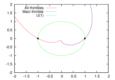
Figure 1: This is the thimble manifold for $\beta=(1+3i)$ and their corresponding plot of $e^{-S_{R}}$, which is proportional to the probability density.

We can take these possibilities for values of $P_{01}(x)$. Then we are restricted by (5) to configurations, where an even number of plaquettes can be $-1$. These configurations clearly fulfill (4).

2.1 Critical manifolds, their tangent spaces and local updates

These are critical manifolds, since our degrees of freedom are still links. We have to compute their Takagi and Anti-Takagis, i.e. vectors, which are solution to the equation

$$H^{*}\Delta z^{*}=\lambda\ \Delta z\>\>\text{with}\>\>\lambda\in\mathbb{R},$$ (7)

where $H$ is the Hessian of the action. Positive $\lambda$ refer to thimble directions, negative $\lambda$ to anti-thimble directions and $\lambda=0$ refers to zero-modes, which come e.g. from the gauge degrees of freedom (see e.g. [4, 12]). For our selection of critical manifolds $P_{i}=\pm 1$ the Hessian splits into a real matrix with a complex prefactor $H=\beta M$, whose eigenvectors $v$ and eigenvalues $\alpha$ can be computed. For $\alpha\neq 0$ we get for the Takagis

$$\Delta z=\sqrt{\frac{\pm\mathrm{sign}(\alpha)\beta^{*}}{|\beta|}}v,$$ (8)

where the sign denotes, if it is a Takagi or Anti-Takagi vector.
We observe, that our Hessian is independent from the actual configuration in the critical manifold. Therefore, we can deduce that the projection of the subspace spanned by its zero modes in the Lie algebra is the critical manifold itself.

$$\left\{U_{\mu}(x)^{\mathrm{crit}}=U_{\mu}(x)^{\mathrm{crit},0}\exp\left({i\sum_{k=1}^{\#(\alpha=0)}c^{k}v^{x,\mu}_{k}(\alpha=0)}\right)\;\;|c^{k}\in\mathbb{C},\;\mu\in\{0,1\},\;x\in\Lambda\right\}$$

Normally, we have to choose a gauge orbit of real dimension by allowing only $c^{k}\in\mathbb{R}$, where we can span the thimble using the Takagi directions. For our main critical manifold $\{P_{i}=1\;\forall i\}$, the complex prefactor in (8) is the same for all Takagi modes. By tilting the real zero modes with the same factor, we differ from a gauge orbit, but get a manifold, which still gives the same expectation values for observables invariant under the zero modes. The set of tilted zero modes and Takagis is equivalent to the tilted unit basis. This gives us the possibility to have a local update algorithm on the tangent space. This is naturally computationally far less demanding than sampling on the thimbles themselves. Restricting ourselves to the main critical manifold, the Jacobian is constant and drops out for expectation values. Another reason, why this could be feasible is the closeness of the local tangent space to the thimble in the one-plaquette model (see Figure 2) in their important regions.

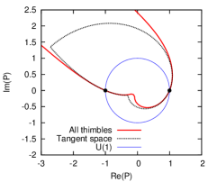
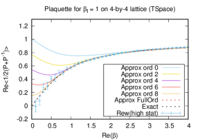
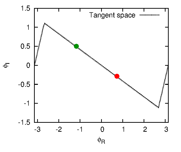
Figure 2: Left: Comparison of the thimbles and their tangent spaces for $\beta=3+3i$. Middle: Thimble hierarchy depending on $\beta_{R}$ in the approximation. Right: Configurations on the tangent space of two plaquettes related to one link.

2.2 Hierarchy of critical manifolds

Our selection of critical manifolds has a natural hierarchy, which is reflected by the values of the action $S=4k\beta,\>\>\>k=0,\ldots,\lfloor{\frac{V}{2}}\rfloor,$ where $k$ is the number of turned plaquette pairs, which are $-1$. With increasing $\beta_{R}$ their weights in the partition sum decrease exponentially. Note that on the thimble the real part of the action becomes minimal at the critical manifold. Consequently for pure imaginary $\beta$, every thimble contributes equally. Otherwise we get a close result by taking into account only a few thimbles, since the others are exponentially suppressed. To get a hint on how strong this is the case, we approximate our model by just taking the leading order contribution of our formal expansion in modified Bessel functions (3)

$$Z=\left[\int_{\mathrm{U}(1)}\mathrm{d}P\ e^{\beta/2(P+P^{-1})}\right]^{V}=\left[I_{0}(\beta)\right]^{V}.$$ (9)

Physically this corresponds to removing periodic boundary conditions. Since this is the One-plaquette model to the power of the volume, we can expand this in term of its thimbles $\mathcal{J}_{0}$, $\mathcal{J}_{1}$

$$Z=\left[\int_{\mathcal{J}_{0}}\mathrm{d}P\ e^{\beta/2(P+P^{-1})}+\int_{\mathcal{J}_{1}}\mathrm{d}P\ e^{\beta/2(P+P^{-1})}\right]^{V}\\ =:\left[Z_{0}+Z_{1}\right]^{V}=\sum_{k=0}^{V}\begin{pmatrix}V\\ k\end{pmatrix}Z_{0}^{V-k}\ Z_{1}^{k}.$$ (10)

Using these, we can calculate approximate values for our observables and their dependence on the thimble hierarchy (see Figure 2).

3 Simulation and comparison

3.1 Algorithm

Since our critical manifolds and tangent spaces depend on the values of the plaquettes, we use them to confine the regions where we sample on them. As one can observe in Figure 2 the two tangent spaces for one plaquette intersect and we can glue them together. This union is homotopic to the orginal $\mathrm{U}(1)$ group. We will use these intersections to limit the region of tangent space we explore. All in all we do a local Metropolis update on the links, where we control the values of the associated plaquettes, preventing them from wandering off the designated main tangent space shown on the right hand side of Figure 2. This is guaranteed by defining that candidates which would land beyond the edges have probability zero and will be rejected by the Metropolis.

3.2 Results for the main tangent space

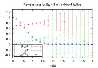
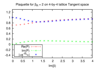
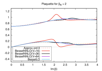
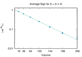
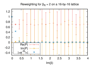
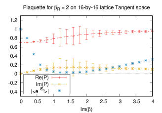
Figure 3: First row: plaquette for $\beta_{R}=2$ with reweighting compared to simulation on the main tangential manifold on a 4 x 4 lattice. Second row: volume dependence of the formal solution and the average sign of the main tangential manifold. Third row: plaquette for $\beta_{R}=2$ with reweighting compared to simulation on the main tangential manifold on a 16 x 16 lattice.

We calculate the expectation value of the average plaquette $<1/2(P+P^{-1})>$. Since $\beta$ is complex, this has a real and an imaginary part. We first note that simulating on the main tangent space alleviates the sign problem in comparison with normal reweighting. Since we only take the main tangent space into account, the results can be considered ’right’ only for large enough beta and sufficiently large volumes. Another thing we note is that for constant $\beta_{R}$, the average sign $|<e^{-iS_{I}}>|$ has a minimum on the $\beta_{I}$ range for every observed volume. So it gets better again for higher $\beta_{I}$.
Looking at this dip at $\beta=2+1.4i$, we look at the volume dependence of $|<e^{-iS_{I}}>|$ using 4-by-4 to 16-by-16 lattices. This seems strictly exponential like it is predicted for the full theory by considering the free energy. But even for a 16-by-16 lattice, where reweighting fails very early for small $\beta_{I}$, we can get a large range where the sign problem is quite mild on the main tangent space. Since higher orders in the modified Bessel function expansion (3) are suppressed by the volume, the leading order approximation coincides stronger with the simulation result.

3.3 Reweighting onto the other tangent spaces

For taking another tangential manifold $\tau_{1}$ into account, e.g. the one related to the critical manifold, where two plaquettes are $-1$, which would be the next one in the hierarchy, we need the ratio $Z_{1}/Z_{0}$ of the partition sums, since we have

$$<\mathcal{O}>_{\tau_{1}\cup\tau_{2}}=\frac{\int_{\tau_{1}}\mathrm{d}U~{}\mathcal{O}[U]e^{-S[U]}+\int_{\tau_{2}}\mathrm{d}U~{}\mathcal{O}[U]e^{-S[U]}}{\int_{\tau_{1}}\mathrm{d}U~{}e^{-S[U]}+\int_{\tau_{2}}\mathrm{d}U~{}e^{-S[U]}}=\frac{<\mathcal{O}>_{\tau_{0}}+(Z_{1}/Z_{0})<\mathcal{O}>_{\tau_{2}}}{1+(Z_{1}/Z_{0})}.$$ (11)

Calculating this, we can follow the method proposed in [13]: Suppose, we have a mapping

$$f\colon\tau_{0}\longrightarrow\;\;\tau_{1}.$$

Then we can write

$$\frac{Z_{1}}{Z_{0}}=\frac{\int_{\tau_{0}}\mathrm{d}Ue^{-S[f(U)]+S[U]}\det[\mathrm{d}f]e^{-S[U]}}{\int_{\tau_{0}}\mathrm{d}Ue^{-S[U]}}=<e^{-S\circ f+S}\det[\mathrm{d}f]>_{0}$$ (12)

The problem here is to find a suitable $f$, which we discuss in our upcoming paper [14]. But we can already say, that since we consider only tangent spaces, $f$ is linear and therefore the Jacobian $\det[\mathrm{d}f]$ is be a constant factor.

4 Summary and Outlook

We have simulated a two dimensional U(1) lattice gauge theory on the tangent space of its main thimble. Hereby, the sign problem is drastically reduced, while the computational complexity has stayed the same as for a local Metropolis update. We proposed taking into account subleading thimbles by a reweighting approach, which is under construction and discussion. We will pursue the technique in the future by looking at other gauge groups including also fermionic determinants and a chemical potential.

References

- [1] P. de Forcrand, Proceedings, 27th International Symposium on Lattice field theory (Lattice 2009): Beijing, P.R. China, July 26-31, 2009, PoS LAT2009, 010 (2009), arXiv:1005.0539 [hep-lat]
- [2] C. Gattringer and K. Langfeld, Int. J. Mod. Phys. A31, 1643007 (2016), arXiv:1603.09517 [hep-lat]
- [3] G. Aarts and I.-O. Stamatescu, JHEP 09, 018 (2008), arXiv:0807.1597 [hep-lat]
- [4] M. Cristoforetti, et al. (AuroraScience), Phys. Rev. D86, 074506 (2012), arXiv:1205.3996 [hep-lat]
- [5] Y. Mori, et al., Phys. Rev. D96, 111501 (2017), arXiv:1705.05605 [hep-lat]
- [6] E. Witten, AMS/IP Stud. Adv. Math. 50, 347 (2011), arXiv:1001.2933 [hep-th]
- [7] K. G. Wilson, Phys. Rev. D10, 2445 (1974)
- [8] R. Balian, et al., Phys. Rev. D10, 3376 (1974), [,74(1974)]
- [9] A. A. Migdal, Sov. Phys. JETP 42, 413 (1975), [,114(1975)]
- [10] J. Berges, et al., Phys. Rev. D75, 045007 (2007), arXiv:hep-lat/0609058 [hep-lat]
- [11] H. Makino, et al., Phys. Rev. D92, 085020 (2015), arXiv:1503.00417 [hep-lat]
- [12] A. Alexandru, et al., Phys. Rev. D93, 014504 (2016), arXiv:1510.03258 [hep-lat]
- [13] S. Bluecher, et al., SciPost Phys. 5, 044 (2018), arXiv:1803.08418 [hep-lat]
- [14] J. Pawlowski, et al., “A local update for pure Yang-Mills theories with a complex coupling ,” In preparation