Design of the Ouroboros packet network

Abstract.

The 5-layer TCP and 7-layer OSI models are taught as high-level frameworks in which the various protocols that are used in computer networks operate.

These models provide valid insights in the organization of network functionalities and protocols; however, the difficulties to fit some crucial technologies within them hints that they don’t provide a complete model for the organization of – and relationships between – different mechanisms in a computer network.

Recently, a recursive model for computer networks was proposed, which organizes networks in layers that conceptually provide the same mechanisms through a common interface. Instead of defined by function, these layers are distinguished by scope.

We report our research on a model for computer networks. Following a rigorous regime alternating design with the evaluation of its implications in an implementation, we converged on a recursive architecture, named Ouroboros. One of our main main objectives was to disentangle the fundamental mechanisms that are found in computer networks as much as possible. Its distinguishing feature is the separation of unicast and broadcast as different mechanisms, giving rise to two different types of layers. These unicast and broadcast layers can easily be spotted in today’s networks.

This article presents the concepts underpinning Ouroboros, details its organization and interfaces, and introduces the free software prototype. We hope the insights it provides can guide future network design and implementation.

1. Introduction

The goal of a network architecture is to organize network functions (mechanisms) in such a way that it reduces complexity, simplifies implementation, operation and management of networks that are designed according to it. This article provides an overview of a new (recursive) network architecture, motivates the functional organization into different components, describes the interfaces between these components and presents a prototype implementation, including some performance indicators.

The first distributed computer communications networks were developed in the 1960s (Baran, 1964; Davies et al., 1967) and, following the rise of the ARPAnet in the early 1970s, structured research into internetwork architectures (networks that interconnect smaller networks) started with the formation of the International Packet Network Working Group (INWG) (McKenzie, 2011) - later designated the International Federation for Information Processing (IFIP) Working Group 6.1 (WG6.1) (Day, 2016). The final proposal for INWG (Cerf et al., 1976) was converging on 3 layers, each with their own transport protocol that included addressing. In the 1980s and into the 1990s, the Open Systems Interconnect (OSI) 7-layer reference model was developed (Zimmermann, 1980; Bachman and Ross, 1982; Day and Zimmermann, 1995; Russell, 2013). The only packet-switched architecture for global networks that is widely adopted and deployed today is a 5-layer model that underpins the Internet, functionally defined through the Transmission Control Protocol / Internet Protocol (TCP/IP) protocol suite (Cerf and Cain, 1983; Postel, 1981a, b).

In contrast to the proposal from INWG, the current Internet follows a catenet model using gateways within a single global network address space (Pouzin, 1974; Cerf, 1978; Postel et al., 1981). Some of the current research questions relating to the TCP/IP Internet hint at inefficiencies at an architectural level. For instance, when TCP segments are sent that are large enough to require IP fragmentation, the loss of any IP fragment requires the entire TCP segment to be retransmitted (Kent and Mogul, 1995). Congestion control is usually implemented in Transport Layer (L4) protocols (Floyd, 2000), such as TCP (Jacobson, 1988), Stream Control Transmission Protocol (SCTP) (Rüngeler et al., 2009), and Datagram Congestion Control Protocol (DCCP) (Floyd et al., 2006). This leaves the IP network vulnerable to congestion (Nagle, 1984) caused by (malicious) programs that use L4 protocols that do not implement congestion control such as the User Datagram Protocol (UDP) (Postel, 1980). QUIC (Langley et al., 2017; Iyengar and Swett, 2018), which is a reliable transport protocol that runs on top of UDP, also implements congestion control. Application programming interfaces (APIs) for networking, such as the socket() interface (Open Group, 2018), require quite some knowledge from the programmer on the protocols used. The socket() interface also requires an update whenever a new protocol is developed (Gilligan et al., 1999), and end-user programs that use the socket() interface will need to be adapted to be able to use any new protocol. Research into more generic programming interfaces for transport networks is ongoing: $\emptyset$MQ (Hintjens, 2013) has been quite succesful as a message interface, and the NEAT project (Khademi et al., 2017) and the IETF Transport Services (taps) Working Group (Pauly et al., 2018) are actively working towards this goal.

Stacking of layers for different network architectures

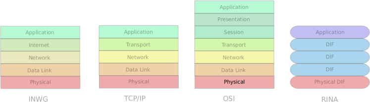
Figure 1. Layers in network architectures

Recent research into network architectures led to the Recursive InterNetwork Architecture (RINA) (Day, 2008; Trouva et al., 2011), which provides a number of key insights on packet networks. RINA reaffirms that communication endpoints are processes, an observation that was also made by early designers of packet networks (Carr et al., 1970; Cerf and Kahn, 1974). It champions a separation of mechanism and policy (Hansen, 1970), separating what is done from how it is done (Dijkstra, 1969). In contrast to defining layers by function (Dijkstra, 1968; Day, 2011), RINA follows an elegant layering paradigm consisting of network layers of identical mechanisms but different policies and/or scope, called Distributed Inter-Process Communication (IPC) Facilities or DIFs (Day et al., 2008). It defines the concept of a flow as the loci of resource allocation necessary to allow the transfer of datagrams from source to destination, rather than identifying a flow as a sequence of packets between a source and destination (Clark, 1988; Tanenbaum and Wetherall, 2010). The recursive structure necessitates a common API to all layers, which – since the scope of a layer spans everything from a single machine to a complete Internet – blurs the line between IPC and networking. Other architectures which follow a similar high-level structure are the Recursive Network Architecture (RNA) (Touch et al., 2006; Touch and Pingali, 2008) and the Dynamic Recursive Unified Internet Design (DRUID) (Joe et al., 2011).

A brief comparison of layering in different architectures is shown in Fig. 1. Throughout this text, layers that are defined by function (protocol) are drawn as boxes, while layers defined by scope are drawn as ovals.

Ouroboros is a novel (recursive) network architecture that incorporates the experience we gained during research collaborations on RINA (Vrijders et al., 2014), as well as a thorough revisiting of a lot of early network research literature that formed the origins for most computer networking concepts. From a high level perspective, Ouroboros looks very similar to RINA, as evidenced by the Rumba (Vrijders et al., 2018) framework, which can be used to deploy the IRATI (Grasa et al., 2013) and rlite (Maffione, 2015) RINA implementations as well as our Ouroboros prototype (Staessens and Vrijders, 2017). The system research approach (Pike, 2000) to building Ouroboros adopts the UNIX design philosophy where each program does one thing well (McIlroy et al., 1978). The end result stems from a number of iterations alternating design and implementation. When compared to RINA, the organization of the mechanisms in the layers is very different in Ouroboros. This warrants considering RINA and Ouroboros as different architectures. We will comment on the most important differences where appropriate and useful.

The main objectives for the Ouroboros architecture are as follows. First of all, it should have no external assumptions on any hardware or operating system environment. Second, we aim to reduce protocol headers to an absolute minimum. Finally, we aim for simple and expressive APIs, hiding complexity as much as possible.

We will now outline the organization of this article, highlighting our contributions. Given that this article details a complete system, it necessarily touches many aspects of computer networks. Core concepts that are needed are detailed in Sec. 2, starting off with some basic definitions from graph theory (Sec. 2.1) and computing (Sec. 2.2), which are used extensively in the remainder of the text. Next, we touch upon naming and addressing in networks. To our taste, an architecture should name every element exactly once, which has led us to question deeply what exactly names and addresses are. Our solution to this question is provided in Sec. 2.3. In computer science literature, there is a distinction between unicast and multicast communication based on whether the communication is one-to-one or many-to-many. Additional distinctions are being made for one-to-any (anycast), and one-to-all, many-to-all and all-to-all (broadcast). The Ouroboros architecture avoids the need to make a distinction between multicast and broadcast, and sees it as a fundamentally different mechanism from unicast. This is based on the simple observation that both the application and the network must be aware that multicast is needed. Ouroboros is – to our knowledge – the first network architecture that clearly separates how it handles unicast from how it handles multicast; putting the functionality into distinct types of network layers. This leads to a solution which finds a middle ground between putting multicast in the network, yet still providing the advantages of using an overlay (Jannotti et al., 2000). The key distinction between these types of layers is based on whether their packet transfer elements implement forwarding, which is defined in Sec.2.4, or broadcast, which is defined in Sec. 2.5. After these more general concepts, we introduce some terminology that are a bit more specific for recursive networks. A lot of these terms were adopted from the RINA architecture to which – as we stated before – Ouroboros is highly indebted. The terms bootstrapping and enrolment are used for adding a node to a network layer, and are explained in Sec. 2.6. A concept of paramount importance is a flow (Sec. 2.7), which is an abstract construct for the network resources that support the unicast transmission of packets between two processes. Flows are provided by (unicast) layers, that consist of a number of processes working together as a distributed application, whereas multicast applications are supported by a broadcast layer (Sec. 2.8). Once a layer is established, it can support flows for higher layers. To make an application reachable over a layer, it must be known to a layer. Sec. 2.9 explains how Ouroboros does this by binding a process to a name, which is then registered in a layer, queriable by a directory service. Processes consist of a collection of logical components (finite state machines), some of which create connections to communicate over a protocol (Sec. 2.10). Exactly how a layer creates a flow to support the connections of higher level applications, is briefly detailed in Sec. 2.11 for local communication; and Sec. 2.12 details how unicast IPCPs create flows over a network layer. The broadcast IPCP that supports multicast/broadcast applications is explained in Sec. 2.13. At this point, all elements are in place to conceptually understand how Ouroboros creates and manages flows. These flows are however not reliable, and are augmented with a reliable transport protocol, providing fragmentation, retransmission, flow control and packet ordering (Sec. 2.14). Sec. 2 continues with sections briefly dealing with Quality of Service (Sec. 2.15) and congestion control (Sec. 2.16). An in-depth overview of the packet processing pipeline (Sec. 2.17) concludes this section., detailing the functions that a packet is experiencing while being forwarded and moving from one layer to the next, using two stripped-down protocols: a data transfer protocol for moving packets between IPCPs, and a transport protocol for the end-to-end functions.

To help the reader get a bit familiar with the concepts, Sec. 3 runs through two examples. The first example (Sec. 3.1) deals with how scalable forwarding is achieved within a layer, while the second example deals with how Ouroboros maintains connectivity for a moving end device connected to different wireless networks (Sec. 3.2).

We delve into the key interfaces that each of the components implements in Sec. 4. The most important is the application programming interface (Sec. 4.1). This interface consists of a small number of minimal and intuitive function calls for establishing and managing flows from within a user program. While unicast and multicast are definitely distinct mechanisms, and applications need to be aware of this, the function calls that are needed are in both cases the same. This is illustrated with 2 short code examples, one outlining a simple unicast application and the other doing the same for a simple multicast application. Currently, programming (IP) multicast applications is far from trivial (Quinn and Almeroth, 2001), we hope our simple API can bring benefits for aspiring multicast application developers. Sec. 4.2 details the flow allocation interface that needs to be implemented by the unicast and broadcast IPCPs, which consists of 6 function calls, out of which the broadcast IPCP only needs to implement 3. Insights on how Ouroboros interfaces with current networks and applications are given in Sec. 4.3.

To become more familiar with Ouroboros, the reference implementation is briefly described in Sec. 5. Its main components are the library (Sec. 5.1) that is used by all Ouroboros applications, the IPC Resource Manager daemon that is the central active component (Sec. 5.2), and the IPCP daemons (Sec. 5.3-5.6) for creating unicast and broadcast layers and for interfacing with the physical network. To get some insights in how to manage an Ouroboros network, we provide a small toolkit that implements the management primitives, consisting of a compact command line interface for creating layers and making applications available over them, detailed in Sec. 5.7. This section is concluded with the description of the ovpn tool that allows connecting IP-based applications over the prototype (Sec. 5.8), a description of other small tools for network testing and demo-ing (Sec. 5.9), and a small example on how to create a 4-node network (Sec. 5.10).

Finally, we summarize our final thoughts and experiences developing and using Ouroboros in our Conclusions, Sec. 6.

2. Concepts

This section defines the concepts that are implemented in Ouroboros, which are common to most – if not all – packet switched networks. This section details a model and deals with (abstract) programs, it does not specify an implementation, and it should not be directly interpreted with respect to any particular implementation of a computing system or environment. The definitions in this section may differ (even ever so slightly) from previously held notions of the term. We address how this academic model can be interpreted towards efficient implementations in Sec. 5.

2.1. Graphs and networks

A graph is a pair $G=(V,E)$ consisting of a set of vertices $V$ and a set of edges $E\subset V^{2}$ of two-element subsets of $V$ (Jungnickel, 2007). An edge $e=\{v_{i},v_{j}\}$ has (distinct) end vertices $v_{i}$ and $v_{j}$. A directed graph or digraph is a pair $G=(V,A)$ consisting of a set $V$ of vertices and a set $A$ of ordered pairs $(v_{i},v_{j})$ (called arcs) where $v_{i}\neq v_{j}$. A network is a digraph $G=(V,A)$ on which a mapping $w:A\rightarrow\mathbb{R}$ from the edgeset to the reals is defined; the number $w(a)$ is called the weight of the arc $a$. If $a=(v_{i},v_{j})\in A$, then $v_{i}$ is adjacent to $v_{j}$ and incident with $a$. The set of neighbors $N$ of a vertex $v$ is the set of vertices that are adjacent to $v$, $N(v)=\{u\in V:(v,u)\in A\}$.

A walk is a sequence of vertices $\mathcal{W}=(v_{0},v_{1},\ldots,v_{n})$ so that $a_{i}=(v_{i-1},v_{i})\in A,i=1,\ldots,n$. So each walk also implies a sequence of edges. We define the weight of a walk $\mathcal{W}$ as the sum of the weights of its arcs, $w(\mathcal{W})=\sum_{i=1}^{n}w(a_{i})$. If the source $v_{0}$ and destination $v_{n}$ are the same ($v_{0}=v_{n}$), the walk is closed. A walk where each of the arcs $a_{i}$ is distinct is called a trail. A path is a trail for which each of the $v_{i}$ are distinct. A closed trail for which the $v_{i}$ are distinct is called a cycle. A directed acyclic graph (DAG) is a digraph that does not contain any cycles. If for every pair of vertices $\{v_{s},v_{d}\}\in V^{2}$ there is at least one path $\mathcal{P}=(v_{s},\dots,v_{d})$, we call the (di)graph connected. The distance function defined by the weight of the shortest path between two vertices in a network (or $\infty$ if no such path exists) is called the geodesic distance. A metric is a (distance) function $d:X^{2}\rightarrow[0,{+}\infty[$ fulfilling positivity, symmetry and triangle inequality: $\forall x,y,z\in X:d(x,y)\geq 0\land d(x,y)=d(y,x)\land d(x,z)\leq d(x,y)+d(y,z)$. A geodesic distance is in general not a metric since it doesn’t always fulfil the positivity and symmetry requirements in a digraph.

2.2. Application, program, process, thread

A program is a (finite) sequence of instructions that can be executed by a computer, designed to solve a specific problem. A process is an instantiation of a program (Tanenbaum and Bos, 2014), and is identified by a process id (PID). Programs may consist of multiple parallel execution threads, identified by a thread id (TID). An application is a collection of processes. A distributed application is a collection of processes residing on different computing systems. The term (computing) system in this text should be interpreted as an implementation of a Turing Machine (Turing, 1936) capable of running the (set of) program(s) that are mentioned with regards to that system. A distributed system is a collection of computing systems that is characterized by concurrency of components, lack of a global clock, and independent failure of components (Coulouris et al., 2011). To us, the lack of a global clock is the only distinguishing feature that really matters.

2.3. Naming and addressing

In most literature on networks, there is a distinction between names, addresses and routes (Postel, 1981a). The ’name’ of a resource indicates what we seek, an ’address’ indicates where it is, and a ’route’ tells us how to get there (Shoch, 1978; Saltzer, 1978).

Distinctions have been made between location-independent names and location-dependent addresses, flat and hierarchical names and – based on whether the name is semantical, i.e. conveys information about the object – pure and impure names (Needham, 1993). What distinguishes an address from a name is oftenly expressed in vague terms, such as “an intermediate form between a name and a route, oriented to machine processing and used to generate the route” (Hauzeur, 1986). A concise definition for an address, that summarizes the perceived consensus in current literature, would probably reflect that addresses are location-dependent, impure synonyms for a resource, usually in the form of a (hierarchically) structured number.

To come to a more precise definition of an address, we will now introduce some concepts using a simple analogy from postal addresses. The authors’ offices are located at “iGent Tower, 126 Technologiepark-Zwijnaarde, 9052, Ghent, Belgium”. Only readers who already know where this is will be able to derive a location from this string, all others will need either a map (an absolute location) or a set of directions (a relative location from his or her current position) to find us. There are two important things to notice.

First, the string is a compound name, composed of names selected from a (non-strict) partially ordered set of namespaces, that are bound to objects from different sets: countries (Belgium), cities (Ghent), postal codes (9052), roads (Technologiepark-Zwijnaarde) and housenumbers (126). “iGent tower” is a synonym for the remainder of the string. The city name is a (not necessarily unique) synonym for a certain group of unique (within the country) postal codes. This strict partial ordering between the named objects (derived from the operator “located within”) is what gives the string a semantic of “location”: Cities are located within countries, streets within cities, and so on.

Second, only one of these substrings is really location-dependent by itself: the housenumber “126”. That is because there is a metric defined on the housenumber namespace from which it is selected. Once in the street, it is trivial to find the house without a map or set of directions. Even more useful is when the names are taken from a normed vector space or coordinate space, denoting an absolute location.

So, in general, we can define an address as a compound name, consisting of names in a non-strict partially ordered set of namespaces that are either metrized or have an associated entity that provides a relative location, allowing to locate an object bound to this name. Elements that have no such metric nor entity associated are synonyms that can be added for human readability, these are not necessary for the purpose of locating the object. These elements are in spaces that are non-strict in the partial order.

In the remainder of this article, when we use the term name, we mean a string without any implied internal structure. The term compound name will be used for strings that consist of names taken from namespaces that have a partial order relationship. For convenience and brevity, if the namespace from which a name was taken has an associated distance function, we will assume it is also coordinate space and use the term coordinate. The reader should keep in mind that wherever the term coordinate is used in the remainder of this article, it can be replaced by “element of a space with associated distance function”.

2.4. Routing and forwarding

Routing is broadly defined as the process of selecting a path for traffic in a network. In computer science literature, there are two main groups of approaches to routing.

On the one hand there is the hierarchical routing solution. This is the approach taken in IP networks, where a set of subnetworks is defined using prefixes or subnet masks (Fuller and Li, 2006). A scalability issue with IP stems from not following the partial ordering implied by the subnetting in the delegation of IP addresses, causing fragmentation of the IP address space (Sriraman et al., 2007) and making prefix aggregration in routers increasingly inefficient.

On the other hand we have geographic or geometric routing (Kuhn et al., 2003), where each node is assigned a coordinate so next hops can be calculated making use of the coordinates of the direct neighbors.

The examples above illustrate that the concept of routing encompasses both the dissemination and gathering of information about the network, and the algorithms for calculation and selection of the paths. We will now define the concepts underpinning “routing” more formally. As far as we know the definitions are original, although the reasoning behind it is similar to the reasoning commonly used in formulating (integer) linear programming solutions to problems in graph theory.

Let $G=(V,A)$ be a network. routing is any algorithm that, given source and destination vertices $v_{s}$ and $v_{d}$, for each vertex $v$ in $V$ returns a subset $H(v)\subseteq N(v)$ of neighbors with the associated set of arcs $L(v)=\{(v,u)\in A:u\in H(v))\}$, so that the following 4 conditions are met: (1) the graph $D=(V^{\prime},A^{\prime})=(\cup_{v\in V}(H(v)),\cup_{v\in V}(L(v)))$ is a directed acyclic subgraph of $G$; (2) $v_{s}$ is the only vertex in $D$ with only outgoing arcs; (3) $v_{d}$ is the only vertex in $D$ with only incoming arcs; and (4) $A^{\prime}=\emptyset$ if and only if there is no path $\mathcal{P}$ between $v_{s}$ and $v_{d}$ in $G$.

Equivalently, routing is any algorithm that, given source and destination vertices $v_{s}$ and $v_{d}$, for each vertex $v$ in $V$ returns a subset $H(v)\subseteq N(v)$ of neighbors so that (1) $\forall{u}\in H(v):d(u,v_{d})<d(v,v_{d})$ for any chosen distance function $d$ on $G$; and (2) $\cup_{v\in V}(H(v))=\emptyset$ if and only if there is no path $\mathcal{P}$ between $v_{s}$ and $v_{d}$ in $G$.

In other words, either the distance function bounds the routing solution, or the routing solution bounds the distance function.

We define forwarding as any algorithm that, for each vertex $v$ in $V$ returns the set of arcs $L(v)$. forwarding is often implemented as routing with an additional edge selection step.

The necessary and sufficient condition for routing is full knowledge of the graph $G=(V,A)$ and a valid geodesic distance $d$. For a given vertex $v$, the necessary and sufficient set of information to obtain $L(v)$ is knowledge of its neighbor set $N(v)$ and the subset of the geodesic distances originating at its neighbors, $d_{v}\subset d:N({v)}\times V\rightarrow\mathbb{R}$. ∎

In less formal terms, routing and forwarding provide a set of vertices and arcs, respectively, so that there are never loops if one travels to a next vertex or along an arc in the set. If implemented in a centralized way, routing and forwarding roughly need to know the full network. When implemented in a distributed way, a node roughly needs to know its neighbors and the distances to the destination from itself and from all its neighbors.

The definitions above show what information needs to be disseminated in a network to allow forwarding. Let’s assume that vertices know their neighbors or incident outgoing arcs, then what is needed is a dissemination procedure for the (geodesic) distance function $d$. This is implemented in a class of dissemination protocols, called distance vector protocols, such as Routing Information Protocol (RIP) (Hedrick, 1988). Each vertex $v$ announces the distances it knows to its neighbors $N(v)$. Border Gateway Protocol (BGP) (Rekhter et al., 2006) is a path vector protocol as it disseminates paths instead of only a distance. This additional information to allow choosing between different available routes based on intermediate nodes or networks.

A different approach is for each vertex $v$ to announce its neighboring links to each of its neighbors $N(v)$, effectively disseminating the full network graph, which allows for more sophisticated routing algorithms. Protocols that follow this approach, such as Open Shortest Path First (OSPF) (Moy, 1998), are called link state protocols.

In Ethernet networks, switches can derive a valid distance function from MAC learning.

The dissemination of information in the network uses network resources, and the convergence time when the graph changes – deletion of a link or vertex due to, for instance, a cable cut or a router power outage – can lead to problems, such as the packets getting stuck in a temporary loop. Let $\mathcal{N}$ a set of names with a bijection $b:\mathcal{N}\leftrightarrow V$ that binds a name $n_{i}$ to a vertex $v_{i}$. For some graphs $G=(V,A)$, a distance function (metric) over namespace $\mathcal{N}$ of vertex names, $d_{\mathcal{N}}:\mathcal{N}^{2}\rightarrow\mathbb{R}$ , can be used to fully infer a valid distance function, $d:V^{2}\rightarrow\mathbb{R}$, over the graph, reducing the need for routing tables and the dissemination of network information (Papadimitriou and Ratajczak, 2005; Kleinberg, 2007).

2.5. Multipoint communication

The definition of routing above intentionally does not include multipoint communication. Unicast and multicast applications must be aware that they are using unicast or multicast communications. Therefore, Ouroboros sees unicast and broadcast as fundamentally different mechanisms, each giving rise to a different type of layer.

broadcast is a trivial well-known algorithm that, for an incoming arc $(i,v)\in A$ of vertex $v$, returns all outgoing arcs $L^{\prime}(v)=\{(v,u)\in A:u\neq i)\}$, with an associated set of vertices $H^{\prime}(v)\subset N(v)=\{w\in V:(v,w)\in L^{\prime}(v)\}$. $H^{\prime}(v)=N(v)$ if $v$ is the source.

It is clear that the graph $G^{\prime\prime}=(V^{\prime\prime},A^{\prime\prime})=(\cup_{v\in V}(H^{\prime}(v)),\cup_{v\in V}(L^{\prime}(v)))=(V,A)=G$ does not fulfill the conditions for a solution to routing unless the input graph already fulfills these conditions.

broadcast is thus mostly used to send information to all network members on a DAG or tree.

2.6. Bootstrapping and enrolment

Bootstrapping is the process of manually configuring a network element to be the first member of a new network layer so it starts its internals to start forwarding or broadcast. Enrolment is the process where an entity contacts (an) existing member(s) of the network to get the necessary configuration information to start its internal components so it can start forwarding or broadcast.

Enrolment is not necessarily a clear-cut procedure or protocol, but may encompass a number of exchanges for getting authentication and encryption keys and configuration information from different sources.

Examples of enrolment in current network are the Wi-Fi association process in 802.11 (IEEE, 1997), and the Dynamic Host Configuration protocol (Droms, 1997) in IP networks. Examples of distributed enrolment are the Spanning Tree Protocol (Perlman, 1985) for Ethernet and the Internet Group Management Protocol (Holbrook et al., 2006) for joining IP multicast networks.

We will illustrate the enrolment process for Ouroboros later in a more practical setting in Sec. 5 when we discuss our reference implementation in detail.

2.7. Flows between processes

A flow is the abstraction of a collection of resources within a network layer that allow bidirectional communications using packets between two processes that are clients of this layer. A flow enables a point-to-point packet delivery service and can be viewed as a bidirectional pipe that has a number of observable quantities associated with it that describe the probability $p(S,t,\ldots)\in[0,1]$ of a packet of given size $S$ being transferred within a certain period of time $[t_{x},t_{x}+t]$. The maximum probability for error-free transfer depends on the packet-drop-rate (PDR) and bit-error-rate (BER) of the flow.

The Ouroboros architecture ensures that flows are content neutral, i.e. the probability $p(S,t,\ldots)$ above is independent of the bits that make up the packets sent along a flow.

The delay or latency describes how long packets take to traverse the flow, and the variation on the delay is called jitter, or more precisely, packet delay variation (Demichelis and Chimento, 2002). The delay for a flow has four main components, propagation and queuing delays, transmission and processing delays.

There are 2 upper bounds, the Maximum Packet Lifetime (MPL) is the maximum amount of time that a packet can take to transfer over the flow, and the Maximum Packet Size (MPS) is the maximum length for a packet to be acceptable for transfer. In other words, the probability for a packet to arrive after MPL expires should be 0, and the probability for a packet to arrive that exceeds the MPS is equal to 0. Similarly, there can be lower bounds such as Minimum Packet Lifetime (mPL) and Minimum Packet Size (mPS).

The resources that make up a layer are finite, limiting the total number of packets that can traverse the network layer in a given period of time. Flows provide the mechanism to put a network layer fully in control of its own resources. The resources that constitute the flow can either be shared with other flows or dedicated (reserved) for this particular flow.

Other externally measureable quantities can be associated with a flow, such as bandwidth and load for flows with reserved resources. The probability function may depend on these quantities (e.g. if the load reaches a certain threshold, delay could increase).

A flow endpoint is identified in a system by a flow ID (FID), which defines the layer boundary. For security reasons, a process has no direct access to the flow, but rather accesses the flow through a Flow Descriptor (FD) to read and write from a flow. Flow identifiers are unique within the scope of a system, flow descriptors are unique within the scope of a process.

Flows are an important concept for enabling Quality-of-Service (QoS) in a layer, which we detail later in Sec. 2.15.

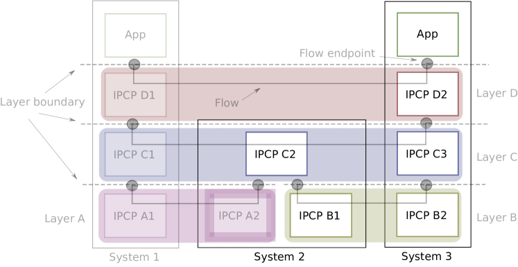
IPC Processes in different layers on different systems

Figure 2. Layers of unicast IPC processes

2.8. Layers of processes

The layering in Ouroboros follows RINA in its fundamental observation that a layer is a collection of processes that form a distributed application. The processes that make up a network layer are called IPC processes (IPCPs). Ouroboros has 2 distinct types of IPCPs to build the recursive network: unicast IPCPs that implement forwarding and provide flows, and broadcast IPCPs that implement broadcast. They both provide a packet delivery service to the processes above, making use of unicast flows provided by the network layer below. Broadcast layers will usually be the top layer in a certain system. This induces (strict) partial order relationships between the IPCPs in a system and between network layers in a network (Fig. 2), which allows us to represent dependencies between layers and and dependencies between IPCPs as directed acyclic graphs (DAGs).

In order to be able to provide flows, a unicast layer has to be capable of at least two basic functionalities: maintaining a directory that keeps track of the location (an IPCP address) where a certain destination process is available, and forwarding packets to this location with non-zero probability of arriving within an appropriate timeframe.

2.9. Binding and registering

The management component of Ouroboros is the IPC Resource Manager (IRM), which provides an interface for administration and configuration of the IPC resources (IPCPs, flows, …) within a system. The IRM is also in charge for delegating outgoing flow requests to layers and assigning incoming flow requests to processes.

Ouroboros binds processes to a name, that can be registered in a layer, populating its directory. These names are given to rather hard-to-define objects – a set of flow endpoints that may be created in the future – therefore we will consider the name to be this very abstract object and use a different font for it. Binding and registering are operations that are (usually) performed by an administrator, not the application programmer, which greatly simplifies writing distributed programs for Ouroboros. The IRM keeps a mapping between PIDs and names, and the layer keeps a mapping between hashes of these names and their locations. These mappings are many-to-many, so a PID can be bound to multiple names and multiple processes can be bound to the same name. Similarly, multiple names can be registered at the same location and a name can be registered at multiple locations (anycast). These bindings are also dynamic during the process runtime, so it is easy to create a running server process, test it over a private network, and then make it available over a public network. All without touching the running server.

The operations do not need to be performed in any particular order, although binding a process will of course only be possible after the process is running. We also allow binding programs to a name, that will cause all future instances of this program to be bound to that name.

Two processes containing partially ordered protocol machines which use a flow to communicate

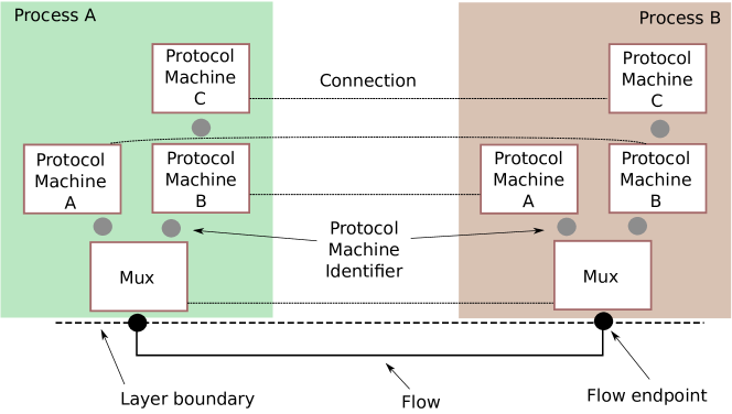
Figure 3. A partially ordered set of protocol machines using a flow (simplified)

2.10. Connections between protocol machines

Processes can be abstracted mathematically as a set of finite state machines (FSMs). A pair of FSMs that communicate using the packet delivery service that is enabled by a flow are called protocol machines (PMs). The communication between two protocol machines at each end of a flow is called a connection. A protocol machine is identified by a protocol machine identifier (PMID) (Fig. 3).

In its full generic form, the Ouroboros architecture exactly mirrors the inter-layer relationship between processes in a system (a strict partial order of IPCPs) to the intra-layer relationship between protocol machines (a strict partial order of PMs). The naming hierarchy of PIDs all the way to FIDs and FDs is copied to PMIDs all the way to connection identifiers (CIDs) and connection descriptors (CDs). Similar to an IRM that manages flows within a system, the Connection Manager (CM) manages connections within a process. This allows full dynamic creation of protocol machines in processes without any statically configured state.

Dynamic allocation of protocol machines in a process is useful only in the most complex and elaborate distributed applications. We will present a simplified version, in line with common practice in protocol design, assuming a static allocation of these identifiers and a static order of the protocol headers, and leave the complete description of this part of the architecture as an exercise to the reader.

In this simplified form, protocol machines at the same level in the partial order are identified using a simple protocol machine called a multiplexing protocol machine or multiplexer using a static PMID as its invariable field; it is not modified during the lifetime of the packet. A multiplexer consists of two classifier FSMs that share state.

Each protocol machine will process its associated packet header and deliver the packet to the next (protocol) state machine downstream/upstream in the DAG.

Some of the protocol machines can be short-lived and bypassed after certain conditions are met (for instance, protocol machines performing configuration or authentication).

It is quite common (and useful) to view a set of protocol machines that depend on each other in a linear hierarchy as a single entity during implementation. In this article, we will also consider some multiplexers as part of other protocol machines to avoid overcomplicating the explanation.

2.11. Flow allocation

The procedure with which a process requests a unicast flow to another process is called flow allocation. A flow is (usually) identified by two flow endpoints, created by the end-hosts’ IRMs, and identified by their flow IDs. The flow IDs allow access to shared state between the IRM, and the two processes, and are unique within a system. Flow endpoints have some minimal resources associated with them, most importantly an incoming rx FIFO and outgoing tx FIFO for packet processing.

The sequence of steps needed for local flow allocation

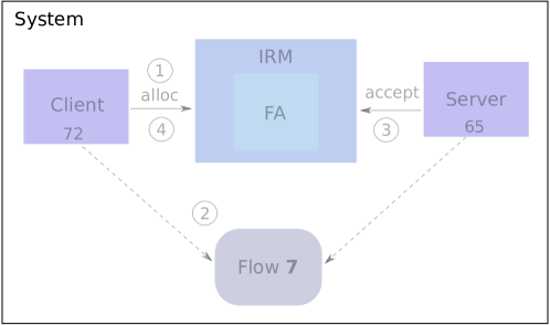
Figure 4. Flow allocation (local)

Fig. 4 illustrates local flow allocation, (i.e. between two processes on a single system), which needs only one flow endpoint, over which the two processes communicate directly. Flow allocation over a layer is explained in Sec. 2.12.2.

We assume the server running as PID $2000$, bound to the name “server” and is calling accept(). The client first calls alloc() to request the IRM for a flow to the name “server” (1). The IRM knows a process (PID 2000) that is bound to that name, and creates a flow endpoint for the flow (2). The accept() call and the alloc() call return at the server and client respectively (3) and (4). The client and server can now communicate over the flow.

The attentive reader may now ask her- or himself how the client process communicates with the IRM, because that is also IPC. This is where we venture into the realm of operating systems. In the ideal implementation, the IRM would be part of the operating system kernel. In that case the calls between processes and the IRM can be either implemented as a system call in a monolithic kernel, or as an IPC mechanism that is bootstrapped between the IPC facility in a microkernel and each process it spawns. Our current (user-space) implementation resorts to UNIX sockets for IPC with the IRM.

The use of the Ouroboros paradigm as the single unifying packet transport technology in (distributed) operating system design is a particularly interesting area for further study. Previously developed distributed operating systems had their own specific protocol for communication between kernel components, and supported TCP/IP in userland. Examples are the special-purpose transport protocol between kernels in Sprite (Ousterhout et al., 1988), the Fast Local Internet Protocol (FLIP) (Kaashoek et al., 1993) used in Amoeba, and the Internet Link (IL) protocol (Presotto and Winterbottom, 1995) used in Plan 9 from Bell Labs.

2.12. The basic functions in the unicast IPC process

We will now present the key protocol machines that implement the basic unicast layer functionality (the directory service, packet forwarding, enrolment and flow allocation) in an Ouroboros IPCP. We further simplified this model in the Ouroboros reference implementation (Sec. 5.3), however it is good to be aware of this more general structure.

The protocol machines in the unicast IPC process

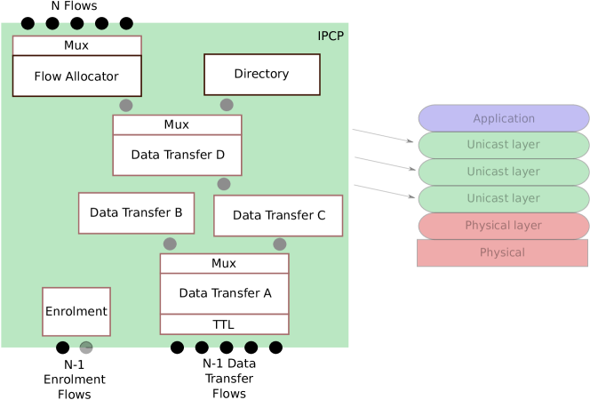
Figure 5. Protocol machines in the unicast IPC process

2.12.1. The directory

The destination for a flow is a name that is registered in the network, it denotes that the IRM of this system is aware of this name and that it can delegate flows to that name to processes on this system. The directory is the entity that maps endpoint names to addresses within a layer. A name can be registered on different addresses, and different names can be registered at the same address. The directory resolves a name to a single address (unicast or anycast, multicast is detailed in Sec. 2.5). To improve security, a layer registers hashes instead of plain-text names (the hash algorithm used is configurable). SHA3-256 (Bertoni et al., 2013; Chang et al., 2012) is used as a default in the implementation, and we will use this algorithm in this article when we mention hashes. Hash values are written as the first 8 characters of their hexadecimal notation. A directory can be implemented as a database (central, replicated, hierarchical or distributed) or as a (distributed) hash table (Sec. 5.3).

The directory is also the entity that provides the mechanism to support anycast: at the address resolution step, if there are multiple destination addresses associated with a certain name, it will return one of these names.

The sequence of steps in flow allocation on two systems

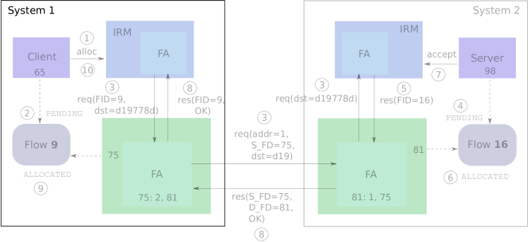
Figure 6. Flow allocation over a layer

2.12.2. Flow allocator

We will illustrate flow allocation over a layer using a (simplified) example where a client on system 1 requests a flow to the server process on system 2 (Fig 6). The IPCP on system 1 has address $1$, the IPCP on system 2 has address $2$, the server is running as PID $2000$ on system 2. The server process is registered in the layer under the name “server”. The directory for the layer maps the hash d19778d to the address $2$, the IRM in system 2 will map PID 2000 to the name “server”.

The steps for flow allocation are as follows: (1) The client requests its IRM for a flow to “server”. (2) The IRM creates a new flow endpoint in PENDING state and assigns it an available flow id FID 9. (3) The IRM sends the request on FID 9 for d19778d to the local IPCP, where the FID 9 is mapped to a local FD 75. The flow allocator in the IPCP in system 1 will forward the request on FD 75 to the flow allocator of the IPCP in system 2, which announces the request to its IRM. (4) System 2’s IRM receives the request for a flow to d19778d. It checks if a there is a process available (it finds PID 2000) and creates a flow endpoint with FID 16, in PENDING state, on system 2. (5) The IPCP is notified of the new flow on FID 16, which is mapped to internal FD 81. The Flow Allocator in the IPCP now contains a mapping that local FD 81 is a flow to system 1, FD 75. (6) The IRM sets the flow endpoint in the ALLOCATED state, and the (7) accept call returns to the server, letting it know it now has a new flow with FD 98. (8) The flow allocator in the IPCP on system 2 concurrently responds to the flow allocator in the IPCP on system 1 that the flow request with source endpoint 75 is accepted at endpoint 81 on system 2. (9) The IRM puts the flow in ALLOCATED state and (10) the allocation call for the client returns with FD 65. At this point the client can write/read to/from FD 65 and the server can read/write from/to FD 98.

The procedure illustrates the flow allocation protocol that is used in Ouroboros. The request message contains 4 fields: the source address, the source endpoint, the QoS specification for the flow (not shown in the example) and the destination hash. The reply message contains 3 fields: the source endpoint, the destination endpoint and a response code indicating if the flow was accepted. To make it more future-proof, the flow allocation protocol will most likely benefit from a version field. After flow allocation, both flow allocators at the endpoint IPCPs map a local FD to a remote address, remote FD and QoS.

2.12.3. Data transfer protocol machines

The protocol machines that are responsible for forwarding packets are called data transfer protocol machines (DTPMs); they implement forwarding. The only disseminated state (field in the packet header) associated with a data transfer protocol machine is a data transfer protocol machine name.

An example is given in Fig. 5, for an IPCP with 4 data transfer protocol machines (with names $A$ to $D$), each chosen from a namespace, $\mathcal{A}$, $\mathcal{B}$, $\mathcal{C}$ or $\mathcal{D}$, consisting of uppercase letters, identified by a multiplexing machine. This directed acyclic graph structure between DTPMs – a generalization of the “hierarchical address spaces” commonly found in literature – defines the protocol headers shown. The operation is simple: if the name in the header matches the name of the PMID, it delivers the packet to the state machine above, else it sends the packet on the flow identified by forwarding. This IPCP functions as a pure router for the address space that contains the namespaces $[A-Z]$.$[A-Z]^{\mathcal{B}}$ (this system cannot allocate flows over DTPM B), and as a possible end host over DTPMs for the address space $[A-Z]$.$[A-Z]^{\mathcal{C}}$.$[A-Z]$. There should not be any packets with address $A$.$B^{\mathcal{B}}$ (since this IPCP can’t provide flows for this address space). Packets with address $A$.$C^{\mathcal{C}}$.$D$ will be delivered to the directory or flow allocator. This sheds some light on the question “Which network entity should be given an address?”. The Ouroboros model defines an address precisely as “a compound name consisting of data transfer protocol machine names, where the (non-strict) partial ordering of the transfer protocol machine namespaces from which these are taken reflects the strict partial ordering of the data transfer protocol machines within an IPC Process”.

This structure does not imply that only pure hierarchical addresses are possible. For instance, techniques like longest prefix matching can be modeled as multiple forwarding FSMs that operate on the same header space, where some treat a compound namespace as a single flat namespace. In the remainder of this article, when we say that some IPCP has address X.Y.Z it means that there are data transfer protocol machines associated with names X, Y and Z inside this IPCP.

2.12.4. Enrolment

This component is responsible for enroling into a new layer, and for accepting enrolment requests from possible new members when already enroled in a layer. Enrolment goes directly over an ephemeral point-to-point N-1 flow that is usually deallocated after enrolment completes. Optimizations may keep this flow for data transfer.

2.13. The basic functions in the broadcast IPC process

Multicast applications are supported using a broadcast layer, for which its IPCPs have a single packet transfer component that implements broadcast, in addition to an enrolment component. The scope of the broadcast layer defines the scope for the multicast application, so usually there will be a broadcast layer for each multicast “stream” (although for instance audio/video streams could be separated in the application since the scope is the same for both).

The protocol machines in the broadcast IPC Process

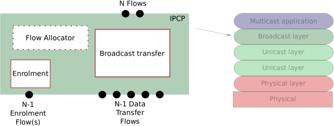
Figure 7. Protocol Machines in the broadcast IPC process

The flow allocator in the broadcast IPCP is a small proxy that only implements a local function that responds positively to a flow join request if the destination name is the layer name. Examples of the use of the unicast and broadcast IPCP are shown in Sec. 5.10.

There are two main approaches for implementing the broadcast IPCP. The first is stateless: the packet transfer component does not require a unique name within the layer, and the only data that needs to be exchanged at enrolment is the layer name. Stateless broadcast IPCPs do not add any protocol headers; all they do is read packets from a FD and forward them on all other FDs (this includes the N-flows). Broadcast layers that are stateless must have trees as their connectivity graph, therefore the enrolment procedure could be augmented with a policy to ensure that the connectivity graph of the broadcast layer is a tree; the optimum solution being a Steiner tree (Bezenšek and Robič, 2014).

The second approach is stateful: the topology can be any graph, and the packet transfer component implements a policy to prevent packets to loop in the network. A simple such policy is to give the packet transfer component a name, and add a packet header with a source name and a sequence number. Each stateful broadcast IPCP then maintains a table tracking ¡source, sequence number¿ pairs, so that the packets that travel in loops can be dropped. The stateful approach can be more resilient, but typically consumes more resources in the lower layer.

Note that differentiating between unicast and broadcast IPCPs in the model does not preclude implementations to provide an IPCP that combines the unicast and broadcast mechanisms into one IPCP, but, since the scope of the layer is defined by its set of IPCPs this may prove less useful than it sounds.

2.14. Reliable connection management

From the definitions above, the packet delivery service offered by a flow can lead to lost, corrupted, duplicated or missequenced packets; a flow is – by nature – unreliable. To provide reliable transfer of information, mechanisms are implemented on top of the flow to provide ordering, duplicate detection and retransmission (Automated Repeat-reQuest, ARQ).

A necessary and sufficient condition to achieve reliable transport is to bound three timers: the maximum packet lifetime (MPL), the time to acknowledge a packet (A) and the time after which there will be no more retransmissions (R) for a certain packet (Fletcher and Watson, 1978; Watson, 1981b). This was implemented in a remarkably simple and elegant protocol, called Delta-$t$ (Watson, 1981a). The OSI TP4 protocol (ISO X.224 (11/95), 1995) and the RINA EFCP protocol (Gürsun et al., 2010) are directly based on Delta-$t$. It is important to note that $A$ and $R$ are strict bounds; after they expire, no more acknowledgments (ACKs) or retransmissions may be sent. However, these timers are not deadlines; they do not imply that an ACK or retransmission must be sent before they expire (the protocol must be able to deal with lost ACKs). In TCP, these three bounds are achieved by the Maximum Segment Lifetime (MSL, 120s), the Maximum Retransmission Timeout (MAX_RTO, 240s) and Delayed ACK timeout (500ms) (Braden, 1989).

Ouroboros also implements a protocol based on Delta-$t$, where the MPL bound is obtained from the MPL characteristic for the flow over which the reliable connection protocol machine is running. The values of $A$ and $R$ are internal to this connection.

In addition, Fragmentation and reassembly allows sending pieces of data that are larger than the MPS of the underlying flow that supports it. Fragmentation and reassembly are enabled by default for flows with in-order delivery, and can be (independently) enabled/disabled at the endpoints. Ouroboros assigns sequence numbers per-fragment and uses a two-bit fragmentation scheme, where the first fragment (FFGM) bit indicates that a received packet is the first fragment of a fragmented packet, and a more fragments (MFGM) bit that is set to $0$ on the last fragment of the packet ($10$ indicates a non-fragmented packet, $11$ the first fragment, $01$ an intermediate fragment and $00$ the last fragment). If the flow is unreliable (no retransmission), packets that have lost fragments are usually discarded. If the flow is to support partial delivery of packets (deliver fragments as soon as they arrive), the MFGM bit is simply ignored at the destination.

Flow control manages the resources at the connection endpoints, avoiding that the source sends information faster than the destination can process. Ouroboros currently implements a commonly used window-based flow control scheme by maintaining a right window edge, updated in every packet, that is controlled by the receiver. Other flow control mechanisms exist, such as rate based flow control, but they are usually tailored to specific situations and are not widely used (rate based flow control is useful only for applications for which processing scales linearly w.r.t. input size), but could be added in the future.

The protocol machines involved with connection management on the sending and receiving side

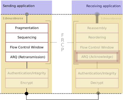
Figure 8. Reliable connection management

Fragmentation, Automated-Repeat-reQuest (ARQ) and flow control are combined in a single protocol, the flow and retransmission control protocol (FRCP) (See Fig. 8).

Ouroboros has the reliable connection state machine as part of every application; it is part of an application library as opposed to as a separate (kernel space) program. The functions that perform error detection, authentication and/or encryption are also provided by the library, but separate from FRCP to allow independent activation and configuration. This is clarified in Sec. 2.17.

2.15. Quality of service

The design of Ouroboros includes 3 mechanisms that allow maintaining a certain Quality of Service (QoS) for a flow.

The first is taking into account QoS requirements in the resource allocation when a flow is established; for instance, by performing bandwidth reservation on a per-flow basis during flow allocation, at step (8) in Fig.6. This is a topic for future study.

The second is differentiated packet handling based on a QoS field in the packet header. Packets with a higher QoS priority can be scheduled accordingly, can be forwarded along different paths and can be handled differently in case of congestion.

The third is the configuration of the FRCP protocol and the integrity/security mechanism in the library. At the application, the specification of the QoS for a flow should be technology-agnostic (Cheong and Lai, 1999). Ouroboros currently defines its QoS specification in terms of delay (ms), bandwidth (bits/s), availability (class of 9s), packet loss rate (packets per billion), bit error rate (errors per billion bits), in order delivery (boolean) and maximum interruption (ms). It should also include authentication and encryption strength; a technology-agnostic way for specifying the trade-off between encryption strength and algorithm complexity is needed. We discuss the application interface in Sec. 4.1 and the implementation in Sec. 5.1.

2.16. Congestion avoidance

Flow control prevents the destination process from being flooded by the sending process, whereas congestion control prevents the network from being flooded by its users (Jain and Ramakrishnan, 1988). Usually, the two functions lend themselves to combined implementations because the underlying mechanism is similar: feedback is used to tune the rate of a flow (Welzl, 2005).

Ouroboros separates congestion control from flow control to ensure that each network layer has full control over its own resources. In essence, both flow control and congestion control do work on the same buffer (the endpoint FIFO to which the application queues outgoing packets), but with flow control it’s the sender application that will limit sending to the FIFO according to its flow control window, and with congestion control it’s the forwarding IPCP in the supporting layer that will limit reading from the FIFO according to its congestion control window. A quick glance at Fig. 9 may help the reader; for a given flow endpoint, the sender tx buffer is the IPCP rx buffer and vice versa.

Congestion avoidance also consists of two different mechanisms: congestion notification, which is implemented in the DTPMs, and the congestion management function that is part of the flow allocator.

In Ouroboros, flow control works on a per-packet basis, while congestion control works on a per-byte basis. The most obvious method for congestion notification is an explicit congestion notification (ECN) scheme. We are currently investigating multi-bit Forward ECN (FECN) approaches modeled on the operation of Data Center TCP (DCTCP) (Alizadeh et al., 2010).

2.17. Packet pipeline

Fig. 9 shows the packet pipeline, representing a model that can be implemented and optimized in a number of different ways depending on the requirements and environment: servers, IoT devices, routers, …will all have very different implementations.

We will explain 3 paths through the pipeline: an application writing to a flow; a packet being forwarded; and an application reading from a flow. The path of the packet is between the endpoints which are a darker shade of grey. We assume the packet passes all steps (most of these steps can be bypassed if they are not needed to achieve the requested QoS). We also assume that there is sufficient credit to send all fragments and only explain the high-level steps, the details of the Delta-$t$ protocol operation are omitted.

The pipeline for processing packets

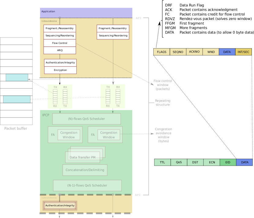
Figure 9. Ouroboros packet processing pipeline

The system stores packets in a large block of packet buffers to avoid copies when the packets are processed by the system, which can be efficiently implemented as a memory pool (also known as a fixed-size block allocator). Each packet buffer allows for head and tail space for adding packet headers when the packet is encapsulated in a lower layer.

When a packet is written to the system using flow_write(), it is first fragmented and the fragments are encapsulated in the FRCP header and put into the packet buffer. The FRCP protocol has a very simple structure, consisting of a sequence number (SEQNO) field, an acknowledgment number (ACKNO) field, a field for updating the (flow control) window (WND) and the payload (DATA), in addition to a FLAGS field containing in total 7 flags, 2 for Delta-$t$: a data run flag (DRF) to indicate there are no unacknowledged packets, and a rendez-vous (RDVZ) packet that is used to resolve a zero window at the sender; 2 for fragmentation (the first fragment FFGM and more fragment (MFGM) bits), and 3 flags that indicate whether the SEQNO, ACKNO and DATA fields are used. If needed, a check or authentication information is appended, let’s assume the packet is encrypted.

Then, the application releases its ownership of the buffer and passes a reference to the buffer to the (next) IPCP, via a FIFO queue (usually implemented as a ring buffer), this is where the layer boundary is crossed.

The lower layer IPCP then reads this packet from the FIFO, via a (N)-flows QoS scheduler that prioritizes the flows. This is also where congestion control is enforced: flows that experience congestion are throttled via a congestion window.

The packet is then encapsulated in a minimalistic data transfer protocol header that consists of only 5 fields: a Time-To-Live (TTL) that ensures that packets don’t live forever in the network and enforces the Maximum Packet Lifetime of the flows, a destination address (DST) so it can be forwarded to the destination, the QoS priority identifier, an ECN field to flag when a flow experiences congestion, and an endpoint identifier (EID) to identify the endpoint at the destination (either an internal component of the IPCP or an N flow, see Sec. 5.6 for more details). The fields are initialized to default values by the Flow Allocator (FA): TTL is set to a certain (configurable) maximum value for the layer, the default is 60 seconds; DST is filled out with the value returned from the directory query; the QoS priority is set according to the QoS specification; and the EID is set according to the value that was agreed during flow allocation, obtained at step (8) in Fig. 6.

The packet is then processed according to the set of DTPMs that corresponds with the QoS priority, possibly concatenated into bigger units to reduce processing in the intermediate nodes, and forwarded on the correct outgoing flow. If the network is getting congested (the packet experiences considerable queuing on the outgoing flow), the ECN field is updated. The concatenation step is located just after the forwarding step to allow concatenation of all packets towards the same destination with the same QoS, limited by the MPS of the outgoing flow.

Packets coming from a lower layer traverse the pipeline in the opposite direction. They are read from the flow and processed by the (N-1)-flows QoS scheduler and passed to the set of DTPMs. If the packet is for a different destination, it is possibly further concatenated and forwarded to the destination.

If the destination address matches the IPCP address, the packet is delivered to the correct protocol machine according to the EID, in our case this will identify an N flow. If the ECN fields are marked, the FA sends a packet to update the sender’s congestion window. The packet is then written to the correct endpoint FIFO, passing the layer boundary, to be read by the application. It passes through decryption and is passed to FRCP, which does bookkeeping of its reception, puts it in order and possibly reassembles it into a full packet before finally delivering it to the application.

Worth noting is that the protocols in Ouroboros do not require a length field. The Heartbleed bug was a well-known example of the potential consequences that an ill-checked length field can have (Durumeric et al., 2014).

3. Examples of the model

This section presents some examples to aid the reader in understanding the model presented in Section 2. These examples are definitely not the only possible solutions within the model.

3.1. Forwarding within a layer

To illustrate the concepts in the model, we provide a small example of forwarding in a unicast layer.

As detailed in Sec. 2.12.3, packets are moved through the network layer via a partially ordered set of DTPMs that implement forwarding. In the example, we assume a total order for simplicity, which allows to use the familiar dotted shorthand notation for the (ternary) compound name that makes up the node address. The node addresses need to be unique within the scope of the layer. Upon receipt of a packet (from an internal component or a flow), the packet will be passed through the DAG of DTPMs.

A network of IPCPs and the path taken from one IPCP to another as well as passing of the packet between protocol machines inside an IPCP

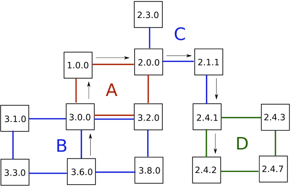
Figure 10. Sending a packet from 3.6.0 to 2.4.2

Fig. 10 shows the example setup. The layer has IPCPs that consist of 3 levels of DTPMs. Each DTPM has an associated dissemination protocol machine (not shown) – for instance, a link state protocol – at its level. For lack of a better term, let’s call a group of dissemination protocol machines that cooperate in a link-state protocol protocol a routing area. Routing areas are defined by the scope of underlying broadcast layers, and the dissemination protocol machines use the broadcast layer for the area. In the case of Fig. 10, the IPCPs with addresses $1.0.0$, $2.0.0$, $3.0.0$ and $3.2.0$ participate in a routing area $A$ at the top level (shown in red). At the middle level, there are 2 routing areas: one consisting of the IPCPs with addresses $3.1.0$, $3.0.0$, $3.2.0$, $3.3.0$, $3.6.0$ and $3.8.0$ (area $B$), and one containing $2.3.0$, $2.0.0$, $2.1.1$ and $2.4.1$ (area $C$). The nodes with address $3.0.0$ and $3.2.0$ are in both areas $A$ and $B$, and $2.0.0$ is in both areas $A$ and $C$. The dissemination protocol at each DTPM level will announce to the participating nodes whether a certain node is also participating at any higher level, which can be done with a single bit. Finally, there is a routing area $D$ at level 3, consisting of the nodes $2.4.1$, $2.4.2$, $2.4.3$ and $2.4.7$.

We now illustrate sending a packet from $3.6.0$ to $2.4.2$. Each DTPM has a complete view of the address, but only makes forwarding decisions within its own level. The IPCP with address $3.6.0$ only participates in the second routing level, which will cause DTPM $6$ to do a check if the address is local (matching all higher level names with the IPCP address: dst $2.X.X$ is not within $3.X.X$). The destination is an address outside the area, so DTMP $6$ will forward to one of the nodes in the area that is marked as participating in a higher level routing area, for instance node $3.0.0$.

Node $3.0.0$ forwards packets at the highest level DTPM, so it sends it to $1.0.0$, which sends it to $2.0.0$ which has 2 as name for its highest level DTPM. Since the highest level DTPM’s name is the same as in the packet, it is passed to the middle DTPM. There the name is different, so it looks in its forwarding table and the packet is sent to $2.1.1$, which forwards it to $2.4.1$. Since the name of the middle DTPM now matches that of the packet, forwarding continues on the lowest DTPM: $2.4.1$ sends it to $2.4.2$. On the IPCP with address $2.4.2$ all DTPM names are matched, so the packet is delivered.

3.2. End-host mobility

Maintaining active TCP connections on mobile hosts is quite challenging. Current solutions – such as in mobile IP (Perkins et al., 1997) and Location-Identifier Separation Protocol (LISP) (Meyer and Lewis, 2013) – rely on establishing tunnels, which puts a significant burden on the tunnel endpoints inside the network, hampering scalability of these solutions.

A key advantage of recursive networks is how they can maintain connectivity for mobile hosts without relying on tunnels, which has recently been demonstrated for RINA networks (Grasa et al., 2018). Our example below will use a slightly different strategy where the end-host does not participate in a dissemination protocol to avoid routing updates. Both approaches are equally valid and can be used in both RINA and Ouroboros.

A figure showing a mobile host moving from WiFi to 4G, showing the layers, IPCPs and addresses of the DTPMs in the IPCP

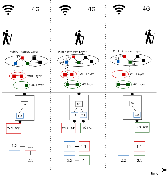
Figure 11. A mobile host switching from WiFi to 4G

Fig. 11 shows a scenario in which a person, using a mobile end host that is connected to a wide area internet layer, moves from an area where access is provided via Wi-Fi technology towards an area where access is provided through a 4th generation (4G) mobile network.

The upper middle section of Fig. 11 shows the network layers that play an important role in mobility. From left to right it shows that the mobile device (blue) keeps its connection in the internet layer by switching from the Wi-Fi layer to the 4G layer using a make-before-break strategy: during the handover it is connected to both the Wi-Fi and 4G network. The lower middle section in Fig. 11 shows the IPCPs in the mobile device, with their flow endpoints. Initially, the mobile device has two IPCPs, a unicast IPCP with address $1.2$ that is enrolled in the internet layer, and a technology-specific WiFi-IPCP that is enrolled in the WiFi layer. By now, it should now be clear that address $1.2$ means that there are actually two DTPMs in a strict order, but we will draw them as a single DTPM and reference to them as a single DTPM in this example to simplify the explanation.

When the host moves, it will detect the 4G network and create another technology-specific 4G-IPCP that connects to the 4G network. The unicast IPCP will be notified of this new 4G IPCP, and allocate a new flow over the 4G network to the public network layer. During the establishment of this new data transfer flow, the mobile host’s public internet IPCP learns that the new gateway has address $2.1$, so it creates a new DTPM which is assigned a compatible address $2.2$. The flow allocator will notify the end host that it now has 2 DTPMs. The flow allocator can now use the 2 DTPMs and may load balance between them. If the Wi-Fi network strength weakens, the unicast IPCP will be notified, and the flow allocator will take action to stop using the Wi-Fi flow and use only the DTPMs with address $2.2$ that is using the 4G IPCP. When the person moves out of reach of the Wi-Fi network, the 4G connection takes over all traffic. In the right panel, the WiFi signal has dropped completely, all flows over this Wi-Fi IPCP are deallocated and tthe WiFi IPCP is destroyed.

The bottom part of Fig. 11 shows a view of the (combined) DTPMs in the unicast IPCP that is enrolled in the internet layer. The middle section makes clear that the network does not view these two DTPMs as part of the same IPCP, because the endpoint doesn’t take part in the dissemination protocol to avoid triggering graph adjacency updates in the network.

4. Interfaces

In this section, we detail the main interfaces in the Ouroboros system and provide an overview of how Ouroboros can run together with current network technologies.

4.1. Application programming interfaces

Ouroboros provides core API interfaces to interact with the system: an application programming interface (API) for Ouroboros applications (user programs, and the unicast and broadcast IPCPs) and a management interface to write tools to manage the networks.

The application interface for inter-process communication (IPC) is split into a synchronous API and a scalable event system based on kqueue (Lemon, 2001). We provide a brief overview of all the function calls in this API (in C syntax (Kernighan and Ritchie, 1988)); for a complete listing of all options, we kindly refer the reader to the man pages that are installed with the Ouroboros package. The API calls for implementing management tools are omitted here (their details are more technical and less important); instead, we explain the management tools in Sec. 5.7. The benefits of the abstractions provided by Ouroboros are reflected in the simplicity of these interfaces.

⬇

/* Returns flow descriptor, qs updates to supplied QoS. */

int flow_alloc(const char * dst, qosspec_t * qs, const struct timespec * timeo);

/* Returns flow descriptor, qs updates to supplied QoS. */

int flow_accept(qosspec_t * qs, const struct timespec * timeo);

/* Returns flow descriptor, qs updates to supplied QoS. */

int flow_join(const char * bc, qosspec_t * qs, const struct timespec * timeo);

int flow_dealloc(int fd);

ssize_t flow_write(int fd, const void * buf, size_t count);

ssize_t flow_read(int fd, void * buf, size_t count);

int fccntl(int fd, int cmd, ...);

Listing 1: Ouroboros application API

The synchronous API, shown in Lst. 1, is fully symmetric. It has functions to allocate unicast flows: a client-side flow_alloc() call and a server-side flow_accept() call; both return a handle to the flow (the flow descriptor, FD). For a broadcast layer, all applications use the flow_join() call, which is similar to flow_alloc(). The flow_alloc() call specifies the QoS for the flow, which is relayed and returned by the server’s flow_accept(). These calls allow specifying a timeout: a time of 0 seconds results in asynchronous allocation where the call will return immediately and allocation will proceed in the background, the result being notified by the event system; NULL waits indefinitely. A flow_dealloc() function allows to release the state associated with a flow. Finally there are the self-explanatory flow_read() and flow_write() calls. These calls are augmented with a “flow and connection control”, fccntl() call that allows configuring some parameters on the flow, such as specifying whether the read and/or write calls are blocking, setting timeout delays for the (blocking) read or write calls, enabling and disabling partial reads, and setting some configuration options for the transport connection, such as disabling fragmentation, reassembly or flow control.

⬇

static void server_main(void)

{

int fd = 0;

char buf[BUF_SIZE];

ssize_t count = 0;

while (true) {

fd = flow_accept(NULL, NULL);

count = flow_read(fd, &buf, BUF_SIZE);

printf("Message from client is %.*s.\n", (int) count, buf);

flow_dealloc(fd);

}

}

static void client_main(void)

{

int fd = 0;

char * message = "Hello World!";

fd = flow_alloc("helloworld-server", NULL, NULL);

flow_write(fd, message, strlen(message) + 1);

flow_dealloc(fd);

}

Listing 2: Ouroboros “Hello World” snippet (unicast)

An example for a simple “hello world” application – a client sending the string “Hello World!” to a server – is shown in Lst. 2. This application assumes that the server code is registered in some layer as “helloworld-server”, which is done outside the application (we explain these steps in a following paragraph). The server (the server_main() function) consists of a simple loop that waits for and accepts a flow, reads a packet from that flow (which it assumes is a string), prints this sentence, and deallocates the flow. The client (the client_main() function) allocates a flow to “helloworld-server”, writes the message “Hello World!” and deallocates the flow.

⬇

static void reader_main(void)

{

int fd;

char buf[BUF_SIZE];

fd = flow_join("helloworld", NULL, NULL);

while (true) {

ssize_t count = flow_read(fd, &buf, BUF_SIZE);

printf("Message is %.*s.\n", (int) count, buf);

}

}

static void writer_main(void)

{

int fd = 0;

char * message = "Hello World!";

fd = flow_join("helloworld", NULL, NULL);

flow_write(fd, message, strlen(message) + 1);/

flow_dealloc(fd);

}

Listing 3: Ouroboros “Hello World” snippet (multicast)

Multicast has a slightly different mode of operation than unicast: the destination is not a server calling flow_accept(), but a broadcast layer, which is reachable using the layer name. The broadcast layer provides a many-to-many packet service, however client applications can easily be restricted to read-only or write-only. The API uses a flow_join() call for broadcast communication.

A multicast example for a simple “hello world” application is shown in Lst. 3. The application uses a broadcast layer called “helloworld”, accessible via the “helloworld” name. Writers access the broadcast layer, write the “Hello World!” string and deallocate the resources. Readers will read from the layer, displaying the “Hello World!” messages from any clients that send it.

⬇

typedef struct qos_spec {

uint32_t delay; /* In ms */

uint64_t bandwidth; /* In bits/s */

uint8_t availability; /* Class of 9s */

uint32_t loss; /* Packet loss, packets per billion */

uint32_t ber; /* Bit error rate, errors per billion bits */

uint8_t in_order; /* In-order delivery, enables FRCT */

uint32_t max_gap; /* In ms */

} qosspec_t;

static const qosspec_t qos_raw;

static const qosspec_t qos_raw_no_errors;

static const qosspec_t qos_best_effort;

static const qosspec_t qos_video;

static const qosspec_t qos_voice;

static const qosspec_t qos_data;

Listing 4: Ouroboros QoS specification

An important mechanism in the API is the ability to set a Quality of Service for a flow in a technology-agnostic way, a possible definition for which is shown in Lst. 4. The struct allows specifying QoS parameters, and a number of these structs have been predefined for convenience. The most important are: two raw QoS services, one that just reads/writes the application packets directly to/from the flow and one that checks integrity (a service similar to UDP); a best-effort QoS that delivers packets in-order; voice and video QoS that add constraints on delay, bandwidth and interruption time; and a data QoS that reliably delivers packets in order. When a flow is allocated, the value of the supplied QoS specification may be updated to the QoS actually supplied to the application.

⬇

oping --server-name oping --interval 0 --count 10000 --quiet --qos raw

--- oping ping statistics ---

10000 packets transmitted, 10000 received, 2 out-of-order, 0% packet loss, time: 577.336 ms

rtt min/avg/max/mdev = 0.033/0.043/1.213/0.039 ms

oping --server-name oping --interval 0 --count 10000 --quiet --qos voice

Server timed out.

--- oping ping statistics ---

10000 packets transmitted, 9995 received, 0 out-of-order, 1% packet loss, time: 2603.373 ms

rtt min/avg/max/mdev = 0.046/0.071/2.773/0.121 ms

oping --server-name oping --interval 0 --count 10000 --quiet --qos data

--- oping ping statistics ---

10000 packets transmitted, 10000 received, 0 out-of-order, 0% packet loss, time: 609.820 ms

rtt min/avg/max/mdev = 0.025/0.048/0.488/0.028 ms

Listing 5: Use of different QoS specifications

An example is given in Lst. 5, where a number of pings (10000) are sent using the Ouroboros ping (oping) application (see Sec. 5.9), where the only difference from the application perspective is that the flow is allocated with different QoS structs as parameters. Because of the multi-threaded nature of the unicast IPCP, packet reordering is possible when sending very fast pings, but there is no packet loss. With a raw QoS specification, the flow delivers all packets, but some arrive out-of-order. With a voice QoS specification, the system will enable in-order delivery and the out-of-order packets will be dropped. A ”Server timed out.” message is displayed showing that the oping client gave up waiting (after 2 seconds) for the dropped out-of-order packets. With a data QoS specification, the system will reorder (and retransmit) packets, leading to complete in-order delivery of all pings sent.

⬇

struct flow_set;

typedef struct flow_set fset_t;

fset_t * fset_create(void);

void fset_destroy(fset_t * set);

void fset_zero(fset_t * set);

int fset_add(fset_t * set, int fd);

bool fset_has(const fset_t * set, int fd);

void fset_del(fset_t * set, int fd);

Listing 6: Ouroboros event system (fset)

Scalable applications need to be able to handle a lot of simultaneous flows, known as the C10k and C10M problem for 10 thousand and 10 million connections to a single server, respectively. Ouroboros provides its own event system API, based on kqueue, to enable writing such applications.

The first part is for managing flows into groups called flow_sets or fsets, and flows can be added or removed from such a set, similar to the FD_SET macros in POSIX, shown in Lst. 6. There are calls to create and destroy an fset, to add or remove an FD from a set, an fset_zero() call to remove all FDs from the set, and an fset_has() call to check if an FD is part of a set. An FD cannot be in multiple fsets at the same time.

⬇

enum fqtype {

FLOW_PKT = 0,

FLOW_DOWN,

FLOW_UP,

FLOW_ALLOC,

FLOW_DEALLOC

};

struct fqueue;

typedef struct fqueue fqueue_t;

fqueue_t * fqueue_create(void);

void fqueue_destroy(fqueue_t * fq);

int fqueue_next(fqueue_t * fq);

enum fqtype fqueue_type(fqueue_t * fq);

int fevent(fset_t * set, fqueue_t * fq, const struct timespec * timeo);

Listing 7: Ouroboros event system (fqueue)

The event system itself operates on these sets. The current events that are supported are: the arrival of a packet on a flow, flow up or down (a failure happened) events, the flow is allocated (for asynchronous flow allocations) or deallocated. The fevent() call waits for events on any flow in a certain fset. It requires an opaque struct, called an fqueue, that upon return of fevent() will hold all FDs for that have some activity on them. The fqueue_next() call traverses these active flows, and the fqueue_type() call can be used to check the type of the current event on the current active FD.

4.2. Flow Allocation Interface

Every IPCP has to implement a set of primitives that constitute the flow allocation API and the management operations. We restrict ourselves to the flow allocation API, shown in Lst. 8, as it provides some insights into what an IPCP has to implement.

⬇

int (* ipcp_reg)(const uint8_t * hash);

int (* ipcp_unreg)(const uint8_t * hash);

int (* ipcp_query)(const uint8_t * hash);

int (* ipcp_flow_alloc)(int fd, const uint8_t * dst, qosspec_t qs);

int (* ipcp_flow_join)(int fd, const uint8_t * dst, qosspec_t qs);

int (* ipcp_flow_alloc_resp)(int fd, int response);

int (* ipcp_flow_dealloc)(int fd);

Listing 8: Flow Allocation Interface

The first two calls are to register and unregister a name at the IPCP, adding or removing a directory entry of ¡hash, IPCP address¿. Ouroboros sends the name information over the API as a hash for security purposes. The IRM of the system learns the hash algorithm for each layer on bootstrap or enrolment. Only unicast IPCPs have to implement the first two functions, in the broadcast IPCP these functions are NULL. The third call queries if a certain name is reachable over a layer, it provides an interface into the directory system, that returns. In a broadcast IPCP, this just checks if the hash matches the broadcast destination.

Then there are three calls that are used to create the actual flow, corresponding to the application API calls, of which the first, ipcp_flow_alloc(), is the most important. Here, the request for a flow is performed, corresponding to step (3) in Fig. 6. The fd parameter is the pending flow that was created by the IRM, the dst parameter is the name of the destination application, (which is resolved to an address from a directory query). The third parameter, the QoS specification qs is the most interesting, as it provides the network with the information that allows it to reserve some network resources for this particular flow. It will also assign a QoS priority that is used in the forwarding (per-priority tables) and scheduling (e.g. to prioritize video over data). The ipcp_flow_alloc_resp() call is invoked when the IRM responds to an incoming requests request, corresponding to step (5) in Fig. 6. This call is not implemented by broadcast IPCPs. Finally, ipcp_flow_dealloc() call releases the local resources, and any network resources associated with the flow. It is an asymmetric function, in that both endpoints of the flow call it, but only the endpoint that allocated the flow will release network resources.

4.3. Interfacing with current network technologies

We will now detail how Ouroboros plugs into existing technologies, which follows similar adoption strategies as outlined for RINA (Vrijders et al., 2013).

There are (at least) 4 pieces of technology that allow Ouroboros to interface with current network infrastructure and applications.

Stacking of Ouroboros layers over OSI layers shown for L1, L2 and L4

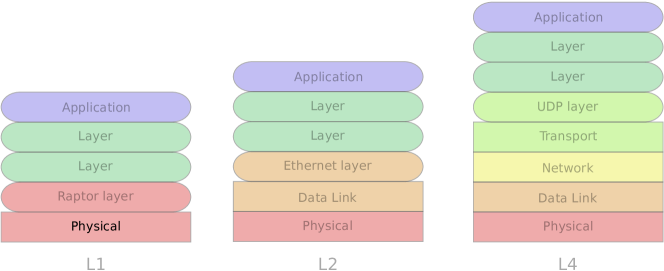
Figure 12. Ouroboros over OSI L1, L2 and L4

First, we can augment current network protocols with a flow allocator to implement the Flow Allocation interface in specific IPCPs which effectively create the lowest layer for the recursive network. This allows to potentially plug Ouroboros into any layer of the OSI model (Fig. 12). We currently have implemented a number of IPCPs to run Ouroboros on top of Layer 1 (a NetFPGA-10G (Lockwood et al., 2007) proof-of-concept called raptor), Layer 2 (Ethernet), and Layer 4 (UDP). These Ouroboros IPCPs are further detailed in Sec. 5.4 – 5.6.

Second, gateways can be implemented between Ouroboros and TCP/IP networks. Such a gateway then listens to the TCP/IP network interface and translates the destination IP address to a name that is known in some layer. Such a gateway application has already been demonstrated for RINA networks (Maffione, 2015; Grasa et al., 2013).

A third piece of technology is to provide an application that exposes a virtual interface and tunnels all traffic on that interface into an Ouroboros network, creating an Ouroboros VPN, similar to the iporinad tool from the rlite project (Maffione, 2015). This is implemented as the ovpn tool, see Sec. 5.8.

Finally, a software adaptation layer is needed to run existing software over Ouroboros without the need for recompilation. A lot of programs are written for the POSIX sockets library, and higher level input/output (I/O) libraries often make use of it, so this is a prime target. A proof-of-concept adaptation layer for POSIX sockets has already been demonstrated for RINA (Williams, 2017).

5. Prototype implementation

Much of the architectural work was performed in tandem with prototype development, to incrementally validate our assumptions and assess the impact of architectural decisions on what we perceived as leading to unnecessary implementation complexity.

The Ouroboros prototype is a user-space implementation (targeted at Portable Operating System Interface (POSIX) compliant operating systems) that aims to be accessible and easy-to-use. It is mostly targeted towards researchers that want to get acquainted with the architecture, as well as free software hobbyists and enthusiasts that are willing to explore new technologies. This choice is further motivated by the ongoing IRATI and rlite efforts to implement RINA, which were already targeting kernel-space implementations for Linux.

The RPC between and linkage of the different software packages

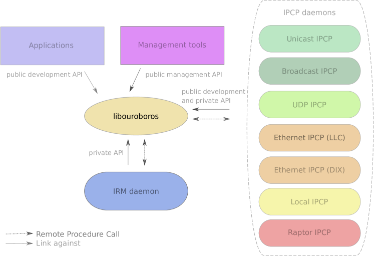
Figure 13. High level overview of the implementation

The implementation consists of a library, the IPC Resource Manager daemon (IRMd), a set of IPCP daemons and a set of tools, as shown in Fig. 13.

The library allows (distributed) applications to communicate over Ouroboros, allows instructing the IRMd with management tools, and implements various utility functions as well as the Remote Procedure Calls (RPC) between the different processes and IRMd in the system.

Then there is the central IPC Resource Manager daemon, which should be considered a part of the operating system. It is the back-end for the management toolset, and also responsible for managing and monitoring applications and IPCPs within the system.

7 IPCPs are currently provided, which are also implemented as daemons. First there are the unicast and broadcast IPCPs that constitute the unicast and broadcast layers, respectively. Then there are 3 IPCPs that allow running Ouroboros over the most used current technologies. One for IP networks that encapsulates in UDP datagrams, and two for Ethernet networks: one using Ethernet II framing and another using Ethernet with Logical Link Control Type 1. A local IPCP is also provided that is similar to a loopback interface and is useful for testing complete networks on a single system. Finally, there is the proof-of-concept Layer 1 IPCP, which we named raptor, that interfaces with a NetFPGA implementation via a (Linux-only) kernel driver.

We also provide a set of tools to manage Ouroboros, that allow users (typically system administrators) to create/destroy IPCPs and create/join network layers, and make applications available over certain layers in the network. Some demonstration applications and general tools are also available as part of the prototype.

5.1. Library

Internally, the library is composed of three parts. First, it contains the common code shared by the prototype. The most important things are the definitions for the RPC messages between the processes and the UNIX sockets interface currently used for relaying these messages. Apart from that, it holds the data structures that are used elsewhere in the implementation, such as a hashtable, a bitmap, various hashing functions and interfaces to external libraries.

Second, it implements the interface for the management tools to send commands towards the IRMd over the UNIX sockets. As before, we don’t go into the details of the management interface, but limit ourselves to describing the tools that are implemented using them (see Sec. 5.7).

Third, it provides interfaces for end-user applications, and IPCPs. The interfaces described in Sec. 4.1 are part of this library. During the execution of the flow_alloc() and flow_accept() calls, the QoS specification is translated into a configuration for FRCP and a decision is made whether or not to add an integrity check. The configuration for FRCP works as follows. If the packets can be delivered out of order, FRCP is completely disabled, which is useful for some simple applications that do not need to run any end-to-end protocol over their links, and also for routers that are designed to handle traffic at line rate. When FRCP is enabled, packets will always be delivered in order. If there can be no packet loss, ARQ is enabled, if there can be no bit errors in a packet, an integrity check is added. These parameters are all signaled end-to-end during flow allocation. If FRCP is enabled, fragmentation, reassembly and flow control are enabled by default, and can be disabled by the end application when needed. The library also takes care of the translation between FID and FD, both for the N flows and the N-1 flows.

One of the key implementation challenges was to implement the functions that are part of the packet processing pipeline, such as the flow and retransmission protocol, so that they are passive functions that are executed in tandem with the I/O or event calls, as opposed to implementing them as an always-active component of the operating system.

To hide most of the implementation details from the API, the RPC interface and the access to data structures in shared memory (the main packet buffer and the tx/rx FIFOs in the flow endpoints) is hidden using init() and fini() functions that are executed automatically when the program initializes and exits, respectively. Since the IRMd creates these data structures, it needs to be started before any applications that use Ouroboros.

5.2. IPC Resource Manager daemon

The IPC Resource Manager daemon (IRMd) is the central management component of Ouroboros. It can be instructed via the management interface for users (typically these would be network administrators). It performs a number of key management and monitoring tasks, such as memory management, application and IPCP management, and flow management.

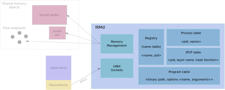
IRMd

Figure 14. The IPC Resource Management daemon

Its memory management task mainly comprises creating the shared data structures that are used for the packet pipeline within the system. When the IRMd boots, it creates a (configurable) fixed-block packet buffer where all packet data is written to. It creates shared datastructures for the event system and flow endpoint FIFOs when needed. Currently, it also creates a UNIX socket over which it listens for new connections for RPC from programs that use Ouroboros. This UNIX socket will be removed in future versions when we bootstrap the RPC over the Ouroboros pipeline.

The IRMd also tracks running processes that use Ouroboros. When these applications start, they send some basic information to the IRMd, such as their PID and the name of the binary (during the init() function in the library). The IRMd needs this information for binding (server) programs to names, so they can accept flows for these names. When a process (identified by its pid) is bound to a name, the IRMd will keep this mapping in its process table. As a shortcut, it also keeps a program table which maps programs to a certain name, so that all future instantiations of that program will be bound for that name. The IRMd can also act as a so-called super-server and start programs for certain registered names if the program that has to accept the flow is known, but not yet running. For this, the program table tracks whether it is allowed to act as a super-server for a particular program and stores the arguments to use when it instantiates a program for a certain name. The IRMd periodically checks if known processes are still alive, so it can clean up stale resources (shared data structures for flows and the event system) when they exit. IPCPs are also processes, so they are also present in the process table, and the IRMd keeps another table for IPCPs that stores some information such as the names of the layers that they belong to and the hash function that each of the IPCPs uses.

For efficiency, it keeps a registry which keeps track of all names known to the system for quick lookups, avoiding the need to search through the process and program tables. Names are added to the registry whenever a new name is registered in a layer or bound to a process or program. This minimizes latency between flow allocations.

The IRMd acts as a broker for outbound and incoming flow allocation requests. For outgoing requests (step (1) in Fig. 6), the IRMd will query the IPCPs in the system for the destination name (using the appropriate hashes) and, if that name is known in the layer, request the IPCP to allocate a flow to that name. For incoming requests (step (3) in system 2 in Fig. 6), the IRMd searches the registry for the name, and if an active process is present in the process table, it will wake up this process (the flow_accept() called by the process will return). If a program for that name is known, the IRMd will first create a process.

Last but not least, the IRMd also acts as a back-end that executes the RPC calls from the management tools that the system administrator uses to create and destroy IPCPs, enrol IPCPs in an existing layer or bootstrap them to create a new layer, list all IPCPs in a system, register and unregister names in a layer, and bind and unbind processes to a name. We detail these operations further in the tools and examples sections.

5.3. Unicast IPC Process daemon

The unicast IPCP daemon performs the tasks needed in order to allocate flows to a certain name making use of existing layers. It provides the flow allocation API towards higher ranked processes, and makes use of the flow allocation API from lower ranked unicast IPCPs. We took two notable shortcuts in the implementation shown in Fig. 15 versus the model in Fig. 5. First, we combined the multiplexing protocol machine on top of the flow allocator (multiplexing to the N-flows) with the multiplexer of the DTPM (multiplexing to the flow allocator and directory). FDs 0-63are reserved to be used for these internal components, larger values indicate N-flows. Second, the TTL protocol machine, QoS multiplexing machine and EID multiplexer are all implemented as a single Data Transfer component. We will now go into a bit more detail of the design decisions for each of the protocol machines in the unicast IPCP. For some of the components (mechanisms), different implementations (policies) are available, to allow tailoring layers to their operating environment.

The protocol machines in the implementation of the unicast IPC process

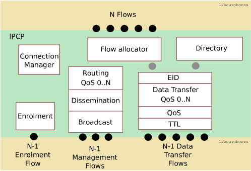
Figure 15. Protocol Machines in the IPC process (implementation)

The connection manager is the component that is in charge of establishing flows for the IPCP (using the flow allocation API). There are three types of flows: enrolment flows, which are used by the enrolment protocol machine during the enrolment procedure, and torn down when enrolment is finished; management flows, which are used by the dissemination protocol machine; and data transfer flows, which are used by the DTPM. After a flow is allocated, the connection managers at the two endpoints will perform a message exchange to determine which component the flow is intended for (flow allocator, data transfer or enrolment), and what common protocol these components will use. Currently, the information that is exchanged between the connection managers contains: the name of the protocol machine, a name for the specific instance (e.g. the DTPM name), and the protocol(s) the instance supports (the protocol machine passes this information as a blob to the connection manager when it starts). Authentication at the process level should take place at this exchange. If the exchange is successful, the connection manager passes the FD for the flow to the correct protocol machine, else the flow is deallocated. The component may authenticate again at the component level. Note that the flow allocator and directory do not have their own flows, but communicate over the Data Transfer component.

The unicast IPCP defaults to a link-state dissemination policy to spread adjacency information in the layer, so that each IPCP can build the graph that it needs for its implementation of routing. These messages contain the link endpoint addresses, the QoS specification of the link, and a sequence number to avoid infinite forwarding and ordering consistency. The collection of LSMs is called the Link State DataBase (LSDB).

The routing instances use the LSDB to calculate next hop neighbors (via a shortest path tree) for each supported QoS priority, which are then used to determine the outgoing FD for each destination address as entries in the forwarding tables used by the DTPM. The routing instances use link weights according to the QoS specifications for the links. There is an option also to calculate Loop-Free Alternates (LFAs) (Atlas and Zinin, 2008) for the different next hops. The forwarding table in the DTPM has two implementations, one that can store a single next hop, and another one that can store alternate next hops for resiliency (such as when using the LFA routing policy).

The DTPM includes the QoS selection PM (to differentiate between different cubes) and on top of a TTL (Time to Live) PM, to discard packets whose TTL is zero. Upon receipt of a packet that is addressed to that DTPM, it will check the endpoint identifier (EID) to see what internal component it is intended for (flow allocator or directory), or write the packet to an N-flow. In the current implementation, DTPMs are assigned a random 32-bit address, as the address space is quite large and the chance at collisions is quite low. Efficient distributed address assignment policies are an interesting topic for future work.

The directory protocol machine implements the resolver for names to IPCP addresses. The default directory implementation is a Distributed Hash Table (DHT) based on the Bittorrent DHT Protocol specification (Loewenstern and Norberg, 2008), which in turn is based on Kademlia (Maymounkov and Mazieres, 2002). The main modifications are support for hash algorithm configuration, which is exchanged during enrolment of the directory (the Kademlia JOIN operation), and that the DHT runs on top of the DTPMs (Kademlia is written specifically for IP networks). The DHT is bootstrapped together with the first IPCP, and new IPCPs try to enrol in the DHT when new Data Transfer flows are created.

In order to monitor the operation of the unicast IPCPs, they can export their full LSDB and a number of statistics for each flow. With statistics output enabled, the unicast IPCP creates a directory in /tmp/ouroboros/ with its name using Filesystems in Userspace (FUSE). For every endpoint (either a flow or internal protocol machine, represented by its FD), it will display some general information, such as the remote endpoint address (in case of a data transfer flow), and a number of statistics such as the number of queued packets and the number of sent and received packets per QoS priority (See Lst. 9).

⬇

Flow established at: 2018-12-30 15:08:17

Endpoint address: 949965593

Queued packets (rx): 0

Queued packets (tx): 0

Qos cube 0:

sent (packets): 213

sent (bytes): 72643

rcvd (packets): 213

rcvd (bytes): 28144

...

Listing 9: Flow statistics (partial output)

The enrolment protocol machine enrols new members in a layer. In case of an enrolment into an existing layer, the enrolment component of the new member will ask its connection manager for a connection to the enrolment component a member of the layer. Once the connection is established, the existing member will send the high-level configuration parameters of the layer. These include the selected policies for the protocol machines, the hashing algorithm of the directory, and the layer name.

5.4. Ethernet IPC Process daemon

Ouroboros provides a number of options to interface with a physical (network) device at the lowest level of the recursive network.

The IPCPs that allow running Ouroboros over Ethernet networks are currently the most used in our lab setup. The first Ethernet IPCP (Fig. 16), referred to as the eth-llc, supports IEEE 802.2 Logical Link Control (LLC) type I over the IEEE 802.3 Ethernet standard. The frame format of LLC is close to the Ouroboros (and RINA) model but we ran into so many issues with LLC support in available equipment – WiFi routers in particular – that we also developed an IPCP over Ethernet DIX, referred to as the eth-dix, which is the preferred choice for easy deployment.

The internal structure of the Ethernet IPCP and its headers

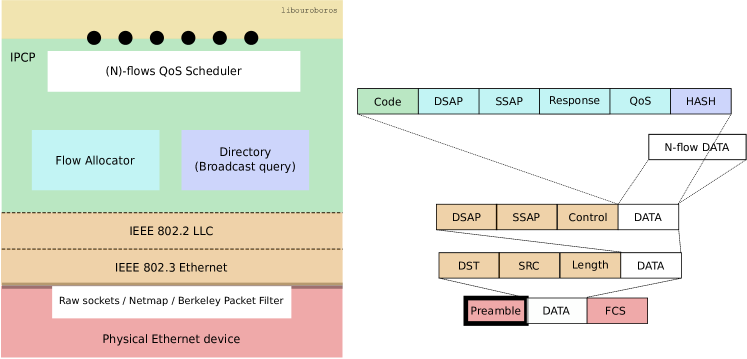
Figure 16. The IPCP over LLC over Ethernet

Both these types of Ethernet IPCPs implement a flow allocator and a directory, which are using a combined (custom) management protocol.

The directory maps hashes to Ethernet MAC addresses, and each IPCP only stores its locally registered hashes. For resolving a hash, the directory function broadcasts a query request message (MAC address FF:FF:FF:FF:FF:FF) containing the requested destination hash. Every Ethernet IPCP (of the same type) that has this hash registered will send a unicast query reply message back to the sender with a positive response; in case of multiple responses, the first one is chosen (anycast). This is similar in function to the Address Resolution Protocol (ARP) (Plummer, 1982), which resolves a generic network protocol address to an Ethernet hardware address. The reason for using a custom protocol instead of ARP is that a lot of Ethernet equipment seems to drop ARP frames if the protocol type is not IPv4 (i.e. the PTYPE field is not 0x0800).

The flow allocators are specific to the flavor of Ethernet. The eth-llc reuses the Service Access Points (SAPs) from IEEE 802.2 as the endpoint ID. The flow allocation requests are sent to a specific Destination SAP (DSAP 0), and flows are then established between two SAPs chosen at the endpoints. The eth-dix IPCP uses an EID, for which it adds an inner header. A configurable non-standardized Ethertype (default 0xA000) is used to identify that the traffic is an Ouroboros Ethernet DIX layer, and that signals that there is an extra inner header present before the actual payload. This Ethertype also serves to run different Ethernet layers in parallel on the same (Virtual) Local Area Network, which is not possible with eth-llc.

To interface with the OS kernels, the Ethernet IPCPs support the raw sockets API of GNU/Linux, and the Berkeley Packet Filter (McCanne and Jacobson, 1993) for BSD and macOS X. They also support netmap (Rizzo, 2012).

5.5. UDP IPC Process daemon

While the Ethernet IPCPs are quite convenient for deploying the prototype in a lab environment, interconnections over larger areas require interworking with IP networks.

Similar to the Ethernet IPCPs, we provide a UDP IPCP, that can transport Ouroboros packets over IP. Technically, we could run Ouroboros-over-IP, but the reason why we use UDP is similar to the reason for creating the eth-llc. Ouroboros-over-IP would need the use of a non-standardized IP protocol, and a lot of available equipment would probably drop such traffic.

The directory function in the UDP IPCPs uses the POSIX interface to resolve hostnames to IP addresses, so it can reuse the existing Domain Name System. Due to restrictions of the lengths of (sub)strings in the DNS standard, the hash function for the directory in the current UDP IPCP is limited to an MD5 hash. Querying for a name is performing a lookup using the hosts file or a (configurable) DNS server. If Dynamic DNS support for the UDP IPCP is enabled, registering or unregistering a name from the UDP IPCP will send a Dynamic DNS (DDNS) request to a DDNS server that adds or removes an entry for the associated MD5 hash.

The flow allocator for the UDP IPCP is similar in function as the flow allocator in the Ethernet IPCPs. Our original implementation of the UDP IPCP reused UDP ports as endpoint identifiers (just like the eth-llc reused SAPs), with a dedicated UDP port to initiate the flow allocation. This, however, led to various deployment issues due to the ubiquitous presence of firewalls and Network Address Translation, which block almost all traffic except for HTTP(S) traffic. For easier NAT and firewall traversal, the UDP IPCP was modified to send all traffic on a (configurable) UDP port, adding an extra inner header containing endpoint identifiers and a length field like the eth-dix. UDP port 443, which is standardized for the QUIC protocol (which is encrypted), is a good candidate to use for tunneling Ouroboros, and therefore our default choice.

5.6. Other IPC Processes

5.6.1. Broadcast IPCP

The broadcast IPCP provided in the implementation is a straightforward implementation of a stateless broadcast layer. A flow join to the name of the broadcast layer will return a flow endpoint to the requesting application from which it can read and to which it can write. The IPCP itself will forward any received packet on all other flows (this includes N-flows for broadcasting to other processes in the same system).

5.6.2. Local IPCP

The local IPCP provides a local loopback function that allows two applications on a single system to communicate over a dedicated link. The local IPCP is very useful for testing, allowing the creation of different networks on a single system.

5.6.3. Raptor

Raptor is a proof-of-concept FPGA demonstrator for running Ouroboros directly over Ethernet PHY (OSI L1). For this, it uses the NetFPGA 10G platform, which has 4 Broadcom AEL2005 PHY 10G Ethernet devices. Raptor consists of three parts: the FPGA design, a Linux kernel module implementing the device driver and a raptor IPCP in userspace. This means that currently raptor only works on GNU/Linux. The raptor IPCP is a very minimal IPCP that is similar to the eth-llc IPCP in its design. However, since Raptor runs point-to-point over Ethernet PHY, and we don’t pursue compatibility with Ethernet networks, it does not need addresses, so raptor’s header consists of a single field: the destination endpoint identifier.

5.7. IPC Resource Management toolkit

The management of recursive networks revolves around the ability to create IPCPs and configuring them to enroll into a certain distributed application – a network layer – so that it can start forwarding or broadcasting packets for client applications.

The hierarchy of IRM tool commands

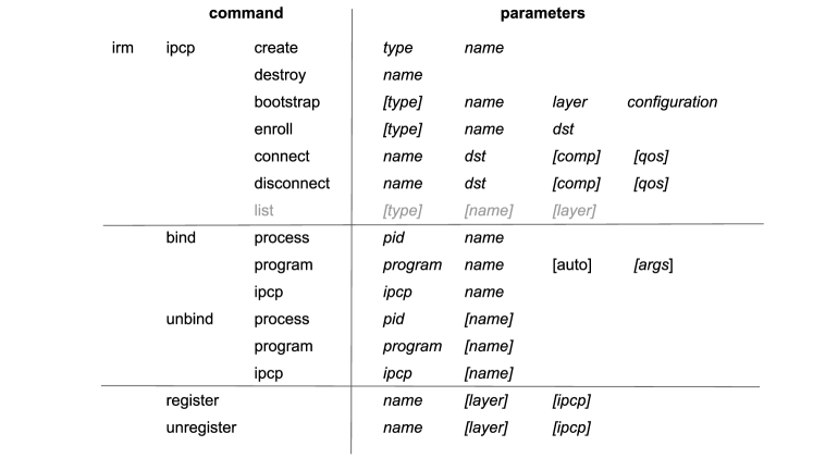
Figure 17. Overview of the command line interface for management

The Ouroboros prototype provides a toolkit that implements the current management interface to create and manage network layers. It provides a command-line interface (CLI) that allows a user (network administrator) to create and destroy IPCPs, list the IPCPs in a system, enroll in network layers, bootstrap new layers, and manage adjacencies in unicast and broadcast layers (Fig. 17). Parameters that are shown between brackets are optional.

IPCPs of a certain type can be created or destroyed with the irm ipcp create name <name> type <type> command. The name of the IPCP should be unique within the layer, and can be used within the system to reference this IPCP. The irm ipcp destroy name <name> command will destroy the IPCP with that name.

To create a new network layer, an IPCP should be bootstrapped, specifying the correct configuration for the layer. Default options are provided to ease configuration. Providing an IPCP type to the bootstrap command is a shorthand to create the IPCP if an IPCP with that name is not yet present in the system. As an example, to create a new layer connected to Wi-Fi on device wlp2s0, the command is irm ipcp bootstrap type eth-dix layer wifi name wifi.0 dev wlp2s0. This will create an Ethernet II IPCP that will capture all traffic on that interface with (default) Ethertype 0xA000 as Ouroboros traffic. To create a new unicast layer named myvpn with default options, the command is irm ipcp bootstrap type unicast layer myvpn name myvpn.0. A listing of these IPCPs on a system is shown in Lst. 10.

⬇

#irm ipcp list

+---------+----------------------+------------+----------------------+

| pid | name | type | layer |

+---------+----------------------+------------+----------------------+

| 31185 | myvpn.0 | unicast | myvpn |

| 31158 | wifi.0 | eth-dix | wifi |

+---------+----------------------+------------+----------------------+

Listing 10: IPCPs in a system

To expand the scope of a layer, new IPCPs can be added to it. For the raptor, eth-dix, eth-llc and udp layers, all IPCPs need to be bootstrapped as the underlying technologies don’t have an enrolment procedure for end hosts. Correctly configuring these IPCPs at bootstrap will add them to the new layer. To expand the scope of a unicast or broadcast layer, new IPCPs need to be enrolled with an existing member. The irm ipcp enrol type unicast name myvpn.1 dst myvpn.0 command will try to enrol the IPCP with name myvpn.1 with an existing member accepting flows for the name myvpn.0. To simplify enrolment, we usually register ipcps with two names: a unique name (e.g. myvpn.0) and the layer name (myvpn), so we can use the layer name (myvpn) as the destination for enrolment (i.e. anycast). As with bootstrapping, providing a type for the enrolment command is a shorthand to create the IPCP if an IPCP with that name does not yet exist in the system. The bootstrap and enrol commands both have an autobind option that will bind the IPCP to two names: the layer name and its IPCP name.

After an IPCP is enrolled, it needs flows to some existing members (adjacencies) over which it can transfer packets. The irm ipcp connect name myvpn.1 dst myvpn.0 command would create two flows between myvpn.1 and myvpn.0, one for data transfer (the adjacency), and one for management (for sending link-state messages). The irm ipcp disconnect name myvpn.1 dst myvpn.0 command can be used to remove these flows.

As a handy tool, the irm ipcp list command can be used to list IPCPs on the system. The optional parameters are to filter the list if many IPCPs are on the same system.

The above commands allow the management of network layers. To make a process reachable over a layer, two steps must be taken: binding that process to a name and registering the name in a layer. The irm bind process 2765 name server command would bind a process with process ID 2765 to the name “server”. We provide a shorthand to bind a certain program to a name: irm bind program /usr/bin/oping name oping.server would bind all future instances of the oping executable to the name oping.server. A similar shorthand is provided for IPCPs so we can use the name that we provided when the IPCP was created. This is to avoid the need to look for the pid of every process that is started. The irm unbind command works the same way. The name is optional: all names for a certain process or binary are unbound if no name is specified.

Finally, names can be registered and unregistered in a layer using the irm register and irm unregister command. These commands usually take a layer name, but if multiple IPCPs of the same layer are present on a single system (for scalability or simply for testing), the name can be registered or unregistered with a specific IPCP.

Note that the order of the commands is not fixed. There is no need to first register and then bind, or vice versa. This is needed to provide as much flexibility as possible.

5.8. Ouroboros Virtual Private Network tool

An important tool is the Ouroboros VPN (ovpn) tool, which allows tunneling IP traffic over an Ouroboros network, similar in operation to the iporinad daemon for RINA networks.

Three systems with their layering and the ovpn application on the two end systems. How it works on a single system is also shown, from a software design point of view.

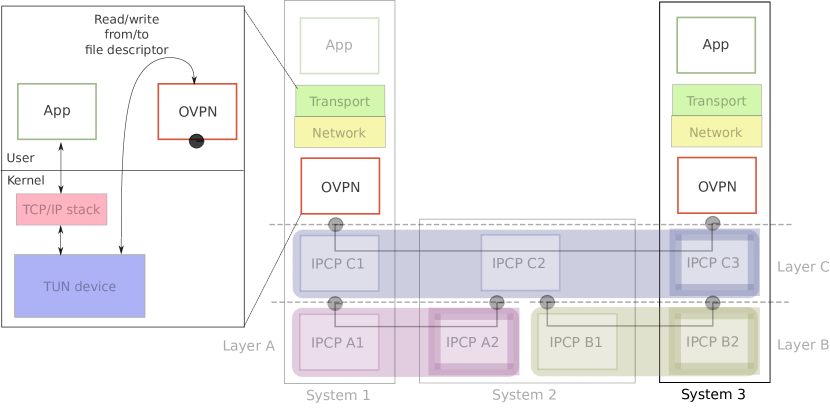
Figure 18. Running IP over Ouroboros with ovpn

The operation of OVPN is shown in Fig. 18. It creates a virtual interface in the host operating system, from which it reads the packets using the POSIX sockets API and writes them to a layer using the flow allocation API provided by Ouorboros. Currently, the OVPN tool creates a so-called tun device, which allows TCP/IP applications to simply use this device like any other IP interface. Administrators can either add a specific routing entry to tunnel the traffic over Ouroboros, or end users can configure their applications to use the tunnel interface’s IP address. The tool allows specifying an IP address and subnet mask to automate the tunnel configuration process.

5.9. Tools

Several small tools are provided together with the Ouroboros implementation.

The oecho tool is a simple application that sends a message to a server which echoes it back. The “hello world” example in Lst. 2 is based on this tool. The ocbr and operf tools allow to perform some unidirectional and bidirectional throughput tests of the prototype. The oping tool allows measuring the round trip time between a client and a server, similar to the well-known ping tool. The obc tool is a simple example of a multicast application running over Ouroboros and is either started as a reader where it receives messages sent to the multicast flow, or as a writer, where it sends messages on the multicast flow. We also provide a patch for the ioq3 engine (id Software, 2012; ioquake3 community, 2012) to run games that use this engine over Ouroboros for demo purposes.

5.10. Examples

To conclude the implementation section, we’ll walk through two examples for creating 4-node network layers, one example demonstrating a unicast layer and one example demonstrating a broadcast layer. We will use the oping application to demonstrate unicast, and the obc application to demonstrate broadcast.

The IPCPs on the different systems and which layers they are using

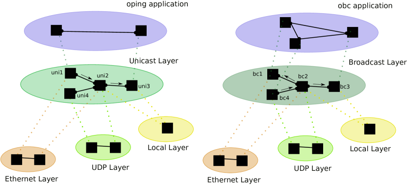
Figure 19. Example scenario for unicast and broadcast

These examples are illustrated in Fig. 19, unicast on the left and broadcast on the right. To demonstrate the use of different layer types for point-to-point connectivity, we will use an Ethernet layer, a UDP layer and a local layer. Using a local layer, we need three systems for this example, labelled $a$, $b$ and $c$. System $a$ is connected to system $b$ over the pure Ethernet layer, system $c$ is connected to system $b$ over a UDP layer on IP subnet 10.1.1.0/24. We will number the IPCPs in the top layer $1$ to $4$, with $1$ residing in system $a$ and $4$ residing in system $c$. The oping server application will be registered at unicast IPCP $3$.

The IPCPs on the different systems and which layers they are using

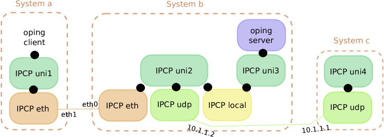
Figure 20. Example scenario (unicast)

This is shown in a bit more detail for the unicast example in Fig. 20. In the following, we assume each system has a running IRMd instance. We will bootstrap the network from system $a$, which connects to system $b$ via a pure Ethernet link via its eth1 Ethernet device. The commands to create the IPCPs in system $a$ are shown in Lst. 11.

⬇

irm ipcp bootstrap name eth layer ethernet type eth-dix dev eth1

irm ipcp bootstrap name uni1 layer unicast type unicast autobind

irm register name uni1 layer ethernet

irm register name unicast layer ethernet

Listing 11: Bootstrapping IPCPs on system $a$

The first command creates and bootstraps an eth-dix IPCP called “eth” in an Ethernet layer on the eth1 interface. This IPCP will provide the data transfer and management flows for the unicast IPCP. The second command creates this unicast IPCP, named “uni1”, and bootstraps it in a layer called “unicast”. The autobind option will bind this IPCP to the names uni1 and unicast (so it is equivalent to adding two irm bind commands). Then both these names are registered in the eth IPCP. After executing these commands, we have two 1-node layers, and uni1 can accept flows to both “unicast” and “uni1” over the Ethernet layer.

⬇

irm ipcp bootstrap name eth layer ethernet type eth-dix dev eth0

irm ipcp bootstrap name udp layer ipnet type udp ip 10.1.1.2

irm ipcp bootstrap name local type local layer local

irm ipcp enrol name uni2 dst unicast autobind

irm ipcp connect name uni2 dst uni1

irm register name uni2 layer ethernet layer ipnet layer local

irm register name unicast layer ethernet layer ipnet layer local

irm ipcp enrol name uni3 dst unicast

irm ipcp connect name uni3 dst uni2

irm bind program oping name oping auto -- -l

irm register name oping ipcp uni3

Listing 12: Bootstrapping IPCPs on system $b$

We will now add the second system, $b$, to the network, and begin with creating the three lower layers. System $b$ connects to the same Ethernet as system $a$ via its eth0 device. The first command in Lst. 12 bootstraps an eth-dix IPCP on the eth0 interface, allowing applications in system $b$ to communicate over Ethernet to system $a$. System $b$ is connected to system $c$ over an IP network, and has IP address $10.1.1.1$ assigned to the connected interface. The second command bootstraps an IPCP over UDP/IP into a layer called ipnet on this interface. Third, it bootstraps a local IPCP for loopback that emulates an internal link. The local layer consist of only this one IPCP.

Now that the lower layers are created in IPCP $b$, the unicast layer can be extended with a new node. To do this, we create a unicast IPCP and enrol it with the IPCP in system $a$. Again, this can be done with a single command, shown on line 4, which creates an IPCP named uni2 and not only enrols the IPCP in the unicast layer, but also binds it to the names “uni2” and “unicast”. After the uni2 IPCP is enroled, we create an adjacency with uni1 so it can forward packets to it. To be able to further extend the unicast layer from system $b$, we register the names “uni1” and “unicast” in all three lower layers. Now that these names are known in the local layer, it is possible to bootstrap the second unicast IPCP in system $b$ and add it to the unicast layer. Note that the enrolment command doesn’t specify which layer it needs to use, the IRMd will select this, and it will first try any IPCPs of type “local”, ensuring the situation in Fig. 20.

We will make the oping application available via the uni3 IPCP. To do this, we bind the program to the name oping and register that in the uni3 IPCP. The bind command uses the auto option, which will make the IRMd in system $b$ act as a super-server for the oping application: if we don’t start an oping server ourselves, the IRMd will start one for us – adding the -l argument – whenever it receives a flow allocation request for the name oping. The unicast layer now has 3 active members: uni1 on system $a$, connected to uni2 on system $b$, in turn connected to uni3 in the same system.

⬇

irm ipcp bootstrap name udp layer ipnet type udp ip 10.1.1.1

echo ’10.1.1.2 869bab4dfd0c0fbedecd374c7089c7a0’ | sudo tee --append /etc/hosts

echo ’10.1.1.2 eebe0851cda7f85aeef4229567441a2d’ | sudo tee --append /etc/hosts

irm ipcp enrol name uni4 dst unicast

irm ipcp connect name uni4 dst uni2

Listing 13: Bootstrapping IPCPs on system $c$

The last step needed in creating our 4-node unicast layer is adding system $c$ to the network (Lst. 13). System $c$ connects to system $b$ over an IP network via the interface with IP address $10.1.1.2$, over which we bootstrap the UDP/IP layer, similar to what we did on system $b$. The unicast IPCP on system $c$ will need to enrol with uni2 on system $b$, which means that the UDP IPCP needs to resolve an address for “uni2” and “unicast”. To keep this example simple to execute we use the hosts file instead of a DDNS server, adding the destination $10.1.1.1$ for the MD5 hashes of the names “uni2” and “unicast”. After adding these two entries, we enrol the new IPCP uni4 and create an adjacency with uni2. The 4-node unicast network layer we set out to create is now fully operational.

⬇

oping -n oping -c 4

Pinging oping with 64 bytes of data (4 packets):

64 bytes from oping: seq=0 time=1.166 ms

64 bytes from oping: seq=1 time=1.083 ms

64 bytes from oping: seq=2 time=1.158 ms

64 bytes from oping: seq=3 time=1.136 ms

--- oping ping statistics ---

4 packets transmitted, 4 received, 0 out-of-order, 0% packet loss, time: 4002.018 ms

rtt min/avg/max/mdev = 1.083/1.136/1.166/0.037 ms

Listing 14: Ping from system $a$ to the oping server

All that remains is to test the network, to do this, we send 4 pings using the oping tool to the oping server (which will be automatically executed on system $b$ once the IRMd on system $b$ receives an allocation request from uni3. The output of executing the oping client is shown in Lst. 14.

The IPCPs on the different systems and which layers they are using

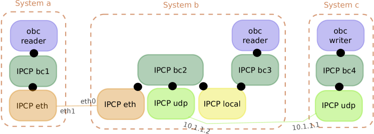
Figure 21. Example scenario (broadcast)

We will now create a similar scenario, but with a 4-node broadcast layer supporting the obc (Ouroboros broadcast) application. There is a reader for the broadcast on system $a$ at IPCP bc1 and on system $b$ at bc3; and a source for the broadcast at IPCP bc4 in system $c$. The scenario is shown in Fig. 21.

⬇

irm ipcp bootstrap name eth layer ethernet type eth-dix dev eth1

irm ipcp bootstrap name bc1 layer broadcast type broadcast autobind

irm register name bc1 layer ethernet

irm register name broadcast layer ethernet

obc -l -n broadcast

Starting a reader.

New flow.

Message is Hello multiple worlds.

Listing 15: Commands on system $a$

The commands are very similar as for the unicast example, so we will just comment on the differences. On node $a$, we create a broadcast IPCP with name “bc1” and bootstrap it into a layer named “broadcast”. The names bc1 and broadcast are then registered in the Ethernet layer. We can already start the receiver at system $a$ in anticipation of the broadcaster.

⬇

irm ipcp bootstrap name eth layer ethernet type eth-dix dev eth3

irm ipcp bootstrap name udp layer ipnet type udp ip 10.1.1.2

irm ipcp bootstrap name local type local layer local

irm ipcp enrol name bc2 layer broadcast type broadcast autobind

irm ipcp connect name bc2 dst bc1 component dt

irm register name bc2 layer ethernet layer ipnet layer local

irm register name broadcast layer ethernet layer ipnet layer local

irm ipcp enrol name bc3 layer broadcast type broadcast

irm ipcp connect name bc3 dst bc2 component dt

obc -l -n broadcast

Starting a reader.

New flow.

Message is Hello multiple worlds.

Listing 16: Commands on system $b$

On system $b$, we bootstrap the lower layers like in the unicast example, enrol and connect a broadcast IPCP bc2 with the bc1 IPCP on system $a$, register the bc2 IPCP in the local layer, and enrol the third bc3 IPCP with bc2. After creating an adjacency between bc3 and bc2, we start the Ouroboros broadcast application to listen to the anticipated broadcast.

Finally, on system $c$, we bootstrap the IPCP over UDP, enrol the final broadcast IPCP with IPCP bc2 on system $b$ and create an adjacency. When we send a message “Hello multiple worlds” using the obc tool, it will be received by the obc clients on systems $a$ and $b$.

⬇

irm ipcp bootstrap name udp layer ipnet type udp ip 10.1.1.1

echo ’10.1.1.2 b605ea609b9dfcf295cfd5a7803dcd37’ | sudo tee --append /etc/hosts

echo ’10.1.1.2 3fecb40eaa447da8f09e6951c7b483f9’ | sudo tee --append /etc/hosts

irm ipcp enrol name bc4 layer broadcast type broadcast

irm ipcp connect name bc4 dst bc2

obc -n broadcast -m "Hello multiple worlds"

Listing 17: Commands on system $c$

6. Conclusions

Today’s computer network technology has sprouted from years of experience in developing and deploying different solutions and making them interoperable through standardization efforts. While the individual mechanisms (congestion control, routing, addressing, …) that are used to build networks are fairly well understood, putting these mechanisms together in a single consistent architecture remains a challenge.

One of the objectives we set when taking on this challenge was to try to contain complexity; minimize as best as we can the impact that some change in one element of the architecture can have on other elements of the architecture; to disentangle as much as possible the elements that make up a computer network. This meant carefully evaluating the implications that making small changes in the architecture have on the implementation and – most importantly – the interfaces between the elements. This approach, combined with the application of a UNIX-like philosophy led to the Ouroboros architecture we detailed here.

The Ouroboros architecture brought us a novel perspective on computer networks; seeing them as flexible ecosystems consisting of 2 distinct types of distributed programs: unicast layers and broadcast layers. These 2 types of layers can easily be observed in todays networks, albeit not isolation: they are often found within a single layer of the Internet model. On the one hand, they can be found in symbiosis: in addition to unicast, Ethernet and IP also support broadcast addresses. On the other hand, they can also be found some intricate entanglement, especially for the purposes of restricting scope: IP multicast groups form a broadcast layer within a unicast layer. It’s interesting to ponder the questions: how much of the complexity is inherent in the layers and how much complexity is added (or subtracted) by entangling them?

The reference implementation has been primarily developed to validate and fine-tune the architecture. However, it is also engineered to present the research community with a set of useful tools to continue exploring various aspects of computer networks.

The architecture and prototype presented in this article are far from complete, they are merely first steps in a direction that – to us – seemed interesting and worthwhile exploring. While we tried to paint as complete a picture as we can from our current vantage point, a lot of it is still distant on the horizon.

References

- (1)
- Alizadeh et al. (2010) Mohammad Alizadeh, Albert Greenberg, David A. Maltz, Jitendra Padhye, Parveen Patel, Balaji Prabhakar, Sudipta Sengupta, and Murari Sridharan. 2010. Data Center TCP (DCTCP). SIGCOMM Comput. Commun. Rev. 40, 4 (Aug. 2010), 63–74. https://doi.org/10.1145/1851275.1851192
- Atlas and Zinin (2008) Alia Atlas and Alex Zinin. 2008. Basic specification for IP fast reroute: Loop-Free Alternates. RFC 5286. IETF.
- Bachman and Ross (1982) Charles W. Bachman and Ronald G. Ross. 1982. Toward a more complete reference model of computer-based information systems. Computer Networks (1976) 6, 5 (1982), 331–343. https://doi.org/10.1016/0376-5075(82)90103-9
- Baran (1964) Paul Baran. 1964. On distributed communications networks. IEEE transactions on Communications Systems 12, 1 (1964), 1–9. https://doi.org/10.1109/TCOM.1964.1088883
- Bellare and Namprempre (2008) Mihir Bellare and Chanathip Namprempre. 2008. Authenticated Encryption: Relations among Notions and Analysis of the Generic Composition Paradigm. Journal of Cryptology 21, 4 (01 Oct 2008), 469–491. https://doi.org/10.1007/s00145-008-9026-x
- Bertoni et al. (2013) Guido Bertoni, Joan Daemen, Michaël Peeters, and Gilles Van Assche. 2013. Keccak. In Advances in Cryptology – EUROCRYPT 2013, Thomas Johansson and Phong Q. Nguyen (Eds.). Springer Berlin Heidelberg, Berlin, Heidelberg, 313–314. https://doi.org/10.1007/978-3-642-38348-9_19
- Bezenšek and Robič (2014) Mitja Bezenšek and Borut Robič. 2014. A Survey of Parallel and Distributed Algorithms for the Steiner Tree Problem. International Journal of Parallel Programming 42, 2 (01 Apr 2014), 287–319. https://doi.org/10.1007/s10766-013-0243-z
- Braden (1989) Robert T. Braden. 1989. Requirements for Internet Hosts - Communication Layers. RFC 1122. https://doi.org/10.17487/RFC1122
- Callon (1996) Ross Callon. 1996. The Twelve Networking Truths. RFC 1925. https://doi.org/10.17487/RFC1925
- Carr et al. (1970) C. Stephen Carr, Stephen D. Crocker, and Vinton G. Cerf. 1970. HOST-HOST Communication Protocol in the ARPA Network. In Proceedings of the May 5-7, 1970, Spring Joint Computer Conference (AFIPS ’70 (Spring)). ACM, New York, NY, USA, 589–597. https://doi.org/10.1145/1476936.1477024
- Cerf (1978) Vinton G. Cerf. 1978. The catenet model for internetworking. Technical Report. DARPA/IPTO.
- Cerf and Cain (1983) Vinton G. Cerf and Edward Cain. 1983. The DoD internet architecture model. Computer Networks (1976) 7, 5 (1983), 307–318. https://doi.org/10.1016/0376-5075(83)90042-9
- Cerf and Kahn (1974) Vinton G. Cerf and Robert E. Kahn. 1974. A Protocol for Packet Network Intercommunication. IEEE Transactions on Communications 22, 5 (May 1974), 637–648. https://doi.org/10.1109/TCOM.1974.1092259
- Cerf et al. (1976) Vinton G. Cerf, Alexander McKenzie, Roger A. Scantlebury, and Hubert Zimmermann. 1976. Proposal for an International End to End Protocol. SIGCOMM Comput. Commun. Rev. 6, 1 (Jan. 1976), 63–89. https://doi.org/10.1145/1015828.1015832
- Chang et al. (2012) Shu-Jen Chang, Ray Perlner, William E. Burr, Meltem Sönmez Turan, John M. Kelsey, Paul. Souradyuti, Lawrence E. Bassham, and Rebecca M. Blank. 2012. Third-Round Report of the SHA-3 Cryptographic Hash Algorithm Competition.
- Cheong and Lai (1999) F. Cheong and R. Lai. 1999. QoS specification and mapping for distributed multimedia systems: A survey of issues. Journal of Systems and Software 45, 2 (1999), 127 – 139. https://doi.org/10.1016/S0164-1212(98)10073-0
- Clark (1988) David D. Clark. 1988. The Design Philosophy of the DARPA Internet Protocols. SIGCOMM Comput. Commun. Rev. 18, 4 (Aug. 1988), 106–114. https://doi.org/10.1145/52325.52336
- Coulouris et al. (2011) George Coulouris, Jean Dollimore, Tim Kindberg, and Gordon Blair. 2011. Distributed Systems: Concepts and Design (5th ed.). Addison-Wesley Publishing Company, USA.
- Davies et al. (1967) D. W. Davies, K. A. Bartlett, R. A. Scantlebury, and P. T. Wilkinson. 1967. A Digital Communication Network for Computers Giving Rapid Response at Remote Terminals. In Proceedings of the First ACM Symposium on Operating System Principles (SOSP ’67). ACM, New York, NY, USA, 2.1–2.17. https://doi.org/10.1145/800001.811669
- Day (2008) John Day. 2008. Patterns in Network Architecture: A Return to Fundamentals. Pearson Education, New York City, New York.
- Day (2011) John Day. 2011. How in the Heck do you lose a layer!?. In 2011 International Conference on the Network of the Future. 135–143. https://doi.org/10.1109/NOF.2011.6126673
- Day (2016) John Day. 2016. The Clamor Outside as INWG Debated: Economic War Comes to Networking. IEEE Annals of the History of Computing 38, 3 (July 2016), 58–77. https://doi.org/10.1109/MAHC.2015.70
- Day et al. (2008) John Day, Ibrahim Matta, and Karim Mattar. 2008. Networking is IPC: a guiding principle to a better internet. In Proceedings of the 2008 ACM CoNEXT Conference. ACM, 67.
- Day and Zimmermann (1995) John D. Day and Hubert Zimmermann. 1995. Conformance Testing Methodologies and Architectures for OSI Protocols. IEEE Computer Society Press, Los Alamitos, CA, USA, Chapter The OSI Reference Model, 38–44. http://dl.acm.org/citation.cfm?id=202035.202039
- Demichelis and Chimento (2002) Carlo M. Demichelis and Philip Chimento. 2002. IP Packet Delay Variation Metric for IP Performance Metrics (IPPM). RFC 3393. https://doi.org/10.17487/RFC3393
- Dijkstra (1968) Edsger W. Dijkstra. 1968. The Structure of the ”THE” multiprogramming System. Commun. ACM 11, 5 (May 1968), 341–346. https://doi.org/10.1145/363095.363143
- Dijkstra (1969) Edsger W. Dijkstra. 1969. The Programming Task Considered as an Intellectual Challenge. https://www.cs.utexas.edu/users/EWD/transcriptions/EWD02xx/EWD273.html
- Dijkstra (1988) Edsger W. Dijkstra. 1988. On the cruelty of really teaching computing science. http://www.cs.utexas.edu/users/EWD/ewd10xx/EWD1036.PDF
- Droms (1997) Ralph Droms. 1997. Dynamic Host Configuration Protocol. RFC 2131. https://doi.org/10.17487/RFC2131
- Durumeric et al. (2014) Zakir Durumeric, Frank Li, James Kasten, Johanna Amann, Jethro Beekman, Mathias Payer, Nicolas Weaver, David Adrian, Vern Paxson, Michael Bailey, and J. Alex Halderman. 2014. The Matter of Heartbleed. In Proceedings of the 2014 Conference on Internet Measurement Conference (IMC ’14). ACM, New York, NY, USA, 475–488. https://doi.org/10.1145/2663716.2663755
- Fletcher (1982) John G. Fletcher. 1982. LINCS: Livermore’s network architecture. Technical Report. Lawrence Livermore Laboratories.
- Fletcher and Watson (1978) John G. Fletcher and Richard W. Watson. 1978. Mechanisms for a reliable timer-based protocol. Computer Networks (1976) 2, 4 (1978), 271 – 290. https://doi.org/10.1016/0376-5075(78)90006-5
- Floyd (2000) Sally Floyd. 2000. Congestion Control Principles. RFC 2914. https://doi.org/10.17487/RFC2914
- Floyd et al. (2006) Sally Floyd, Mark J. Handley, and Eddie Kohler. 2006. Datagram Congestion Control Protocol (DCCP). RFC 4340. https://doi.org/10.17487/RFC4340
- Fuller and Li (2006) Vince Fuller and Tony Li. 2006. Classless Inter-domain Routing (CIDR): The Internet Address Assignment and Aggregation Plan. RFC 4632. https://doi.org/10.17487/RFC4632
- Gilligan et al. (1999) Robert E. Gilligan, Jim Bound, Susan Thomson, and W. Richard Stevens. 1999. Basic Socket Interface Extensions for IPv6. RFC 2553. https://doi.org/10.17487/RFC2553
- Grasa et al. (2018) Edu Grasa, Leo Bergesio, Miquel Tarzan, Diego Lopez, Sven van der Meer, John Day, and Lou Chitkushev. 2018. Mobility management in RINA networks: Experimental validation of architectural properties. In Wireless Communications and Networking Conference (WCNC), 2018 IEEE. IEEE, 1–6.
- Grasa et al. (2013) Eduard Grasa, Francesco Salvestrini, Leonardo Bergesio, Miquel Tarzan, Sander Vrijders, and Dimitri Staessens. 2013. IRATI, a RINA implementation for OS/Linux. https://github.com/irati/stack
- Gürsun et al. (2010) Gonca Gürsun, Ibrahim Matta, and Karim Mattar. 2010. Revisiting A Soft-State Approach to Managing Reliable Transport Connections. In Proceedings of the Eighth International Workshop on Protocols for Future, Large-Scale and Diverse Network Transports (PFLDNeT 2010).
- Hansen (1970) Per Brinch Hansen. 1970. The Nucleus of a Multiprogramming System. Commun. ACM 13, 4 (April 1970), 238–241. https://doi.org/10.1145/362258.362278
- Hauzeur (1986) Bernard M. Hauzeur. 1986. A Model for Naming, Addressing and Routing. ACM Transactions on Information Systems 4, 4 (Dec. 1986), 293–311. https://doi.org/10.1145/9760.9761
- Hedrick (1988) Chuck Hedrick. 1988. Routing Information Protocol. RFC 1058. https://doi.org/10.17487/RFC1058
- Hintjens (2013) Pieter Hintjens. 2013. ZeroMQ, Messaging for Many Applications (1st ed.). O’Reilly Media, Inc.
- Holbrook et al. (2006) Hugh Holbrook, Brad Cain, and Brian Haberman. 2006. Using Internet Group Management Protocol Version 3 (IGMPv3) and Multicast Listener Discovery Protocol Version 2 (MLDv2) for Source-Specific Multicast. RFC 4604. https://doi.org/10.17487/RFC4604
- id Software (2012) id Software. 2012. Quake III Arena GPL Source Release. https://github.com/id-Software/Quake-III-Arena
- IEEE (1997) IEEE. 1997. Wireless LAN Medium Access Control (MAC) and Physical Layer (PHY) Specification.
- ioquake3 community (2012) ioquake3 community. 2012. Free Software FPS Game Engine Based on Quake 3 for Windows, Linux, and macOS. https://www.ioquake3.org/
- ISO X.224 (11/95) (1995) ISO X.224 (11/95) 1995. Information technology - Open Systems Interconnection - Protocol for providing the connection-mode transport service . Standard. International Organization for Standardization, Geneva, CH.
- ISO/IEC 15954:1999 (1999) ISO/IEC 15954:1999 1999. Connection-mode protocol for the Application Service Object Association Control Service Element. Standard. International Organization for Standardization, Geneva, CH.
- Iyengar and Swett (2018) Janardhan Iyengar and Ian Swett. 2018. QUIC Loss Detection and Congestion Control. Internet-Draft draft-ietf-quic-recovery-14. Internet Engineering Task Force. https://datatracker.ietf.org/doc/html/draft-ietf-quic-recovery-14 Work in Progress.
- Jacobson (1988) Van Jacobson. 1988. Congestion Avoidance and Control. In Symposium Proceedings on Communications Architectures and Protocols (SIGCOMM ’88). ACM, New York, NY, USA, 314–329. https://doi.org/10.1145/52324.52356
- Jain and Ramakrishnan (1988) Raj Jain and K. K. Ramakrishnan. 1988. Congestion avoidance in computer networks with a connectionless network layer: concepts, goals and methodology. In [1988] Proceedings. Computer Networking Symposium. 134–143. https://doi.org/10.1109/CNS.1988.4990
- Jannotti et al. (2000) John Jannotti, David K. Gifford, Kirk L. Johnson, M. Frans Kaashoek, and James W. O’Toole, Jr. 2000. Overcast: Reliable Multicasting with on Overlay Network. In Proceedings of the 4th Conference on Symposium on Operating System Design & Implementation - Volume 4 (OSDI’00). USENIX Association, Berkeley, CA, USA, Article 14. http://dl.acm.org/citation.cfm?id=1251229.1251243
- Joe et al. (2011) Touch. Joe, Ilia Baldine, Rudra Dutta, Gregory G. Finn, Bryan Ford, Scott Jordan, Dan Massey, Abraham Matta, Christos Papadopoulos, Peter Reiher, and George Rouskas. 2011. A Dynamic Recursive Unified Internet Design (DRUID). Computer Networks 55, 4 (2011), 919–935. https://doi.org/10.1016/j.comnet.2010.12.016 Special Issue on Architectures and Protocols for the Future Internet.
- Jungnickel (2007) Dieter Jungnickel. 2007. Graphs, Networks and Algorithms (3rd ed.). Springer Publishing Company, Incorporated.
- Kaashoek et al. (1993) M. Frans Kaashoek, Robbert van Renesse, Hans van Staveren, and Andrew S. Tanenbaum. 1993. FLIP: An Internetwork Protocol for Supporting Distributed Systems. ACM Trans. Comput. Syst. 11, 1 (Feb. 1993), 73–106. https://doi.org/10.1145/151250.151253
- Kent and Mogul (1995) Christopher A. Kent and Jeffrey C. Mogul. 1995. Fragmentation Considered Harmful. SIGCOMM Comput. Commun. Rev. 25, 1 (Jan. 1995), 75–87. https://doi.org/10.1145/205447.205456
- Kernighan and Ritchie (1988) Brian W. Kernighan and Dennis M. Ritchie. 1988. The C Programming Language (2nd ed.). Prentice Hall Professional Technical Reference.
- Khademi et al. (2017) Naeem Khademi, David Ros, Michael Welzl, Zdravo Bozakov, Anna Brunstrom, Gorry Fairhurst, Karl-Johan Grinnemo, David Hayes, Per Hurtig, Tom Jones, Simone Mangiante, Michael Tuxen, and Felix Weinrank. 2017. NEAT: A Platform- and Protocol-Independent Internet Transport API. IEEE Communications Magazine 55, 6 (2017), 46–54. https://doi.org/10.1109/MCOM.2017.1601052
- Kleinberg (2007) Robert Kleinberg. 2007. Geographic Routing Using Hyperbolic Space. In IEEE INFOCOM 2007 - 26th IEEE International Conference on Computer Communications. 1902–1909. https://doi.org/10.1109/INFCOM.2007.221
- Kuhn et al. (2003) Fabian Kuhn, Rogert Wattenhofer, Yan Zhang, and Aaron Zollinger. 2003. Geometric Ad-hoc Routing: Of Theory and Practice. In Proceedings of the Twenty-second Annual Symposium on Principles of Distributed Computing (PODC ’03). ACM, New York, NY, USA, 63–72. https://doi.org/10.1145/872035.872044
- Langley et al. (2017) Adam Langley, Alistair Riddoch, Alyssa Wilk, Antonio Vicente, Charles Krasic, Dan Zhang, Fan Yang, Fedor Kouranov, Ian Swett, Janardhan Iyengar, Jeff Bailey, Jeremy Dorfman, Jim Roskind, Joanna Kulik, Patrik Westin, Raman Tenneti, Robbie Shade, Ryan Hamilton, Victor Vasiliev, Wan-Teh Chang, and Zhongyi Shi. 2017. The QUIC Transport Protocol: Design and Internet-Scale Deployment. In Proceedings of the Conference of the ACM Special Interest Group on Data Communication (SIGCOMM ’17). ACM, New York, NY, USA, 183–196. https://doi.org/10.1145/3098822.3098842
- Lemon (2001) Jonathan Lemon. 2001. Kqueue - A Generic and Scalable Event Notification Facility. In Proceedings of the FREENIX Track: 2001 USENIX Annual Technical Conference. USENIX Association, Berkeley, CA, USA, 141–153. http://dl.acm.org/citation.cfm?id=647054.715764
- Lockwood et al. (2007) John W. Lockwood, Nick McKeown, Greg Watson, Glen Gibb, Paul Hartke, Jad Naous, Ramanan Raghuraman, and Jianying Luo. 2007. NetFPGA–An Open Platform for Gigabit-Rate Network Switching and Routing. In 2007 IEEE International Conference on Microelectronic Systems Education (MSE’07). 160–161. https://doi.org/10.1109/MSE.2007.69
- Loewenstern and Norberg (2008) Andrew Loewenstern and Arvind Norberg. 2008. Bittorrent Enhancement Proposal (BEP) 5, Bittorrent DHT Protocol. http://www.bittorrent.org/beps/bep_0005.html
- Maffione (2015) Vincenzo Maffione. 2015. rlite: A light RINA implementation. https://github.com/rlite/rlite
- Maymounkov and Mazieres (2002) Petar Maymounkov and David Mazieres. 2002. Kademlia: A peer-to-peer information system based on the xor metric. In International Workshop on Peer-to-Peer Systems. Springer, 53–65.
- McCanne and Jacobson (1993) Steven McCanne and Van Jacobson. 1993. The BSD Packet Filter: A New Architecture for User-level Packet Capture.. In USENIX winter, Vol. 46.
- McIlroy et al. (1978) Malcolm Douglas McIlroy, Elliot N. Pinson, and Berk A. Tague. 1978. UNIX Time-Sharing System: Foreword. Bell Sys. Tech. J. 57, 6 (1978), 1899–1904.
- McKenzie (2011) Alexander McKenzie. 2011. INWG and the Conception of the Internet: An Eyewitness Account. IEEE Annals of the History of Computing 33, 1 (Jan. 2011), 66–71. https://doi.org/10.1109/MAHC.2011.9
- Meyer and Lewis (2013) David Meyer and Darrel Lewis. 2013. The locator/Id separation protocol (LISP). IETF RFC 6830 (2013).
- Mockapetris (1987a) Paul V. Mockapetris. 1987a. Domain names - concepts and facilities. RFC 1034. https://doi.org/10.17487/RFC1034
- Mockapetris (1987b) Paul V. Mockapetris. 1987b. Domain names - implementation and specification. RFC 1035. https://doi.org/10.17487/RFC1035
- Moy (1998) John Moy. 1998. OSPF Version 2. RFC 2328. https://doi.org/10.17487/RFC2328
- Nagle (1984) John Nagle. 1984. Congestion Control in IP/TCP Internetworks. SIGCOMM Comput. Commun. Rev. 14, 4 (Oct. 1984), 11–17. https://doi.org/10.1145/1024908.1024910
- Needham (1993) Roger M. Needham. 1993. Distributed Systems (2nd Ed.). ACM Press/Addison-Wesley Publishing Co., New York, NY, USA, Chapter Names, 315 – 327.
- Open Group (2018) The Open Group. 2018. IEEE Standard for Information Technology–Portable Operating System Interface (POSIX®) Base Specifications, Issue 7. Technical Report. IEEE. 1–3951 pages. https://doi.org/10.1109/IEEESTD.2018.8277153
- Ousterhout et al. (1988) John K. Ousterhout, Andrew R. Cherenson, Frederick Douglis, Michael N. Nelson, and Brent B. Welch. 1988. The Sprite Network Operating System. Computer 21, 2 (Feb. 1988), 23–36. https://doi.org/10.1109/2.16
- Papadimitriou and Ratajczak (2005) Christos H. Papadimitriou and David Ratajczak. 2005. On a conjecture related to geometric routing. Theoretical Computer Science 344, 1 (2005), 3–14. https://doi.org/10.1016/j.tcs.2005.06.022 Algorithmic Aspects of Wireless Sensor Networks.
- Pauly et al. (2018) Tommy Pauly, Brian Trammell, Anna Brunstrom, Gorry Fairhurst, Colin Perkins, Phillip S. Tiesel, and Christopher A. Wood. 2018. An Architecture for Transport Services. Internet-Draft draft-ietf-taps-arch-01. Internet Engineering Task Force. https://datatracker.ietf.org/doc/html/draft-ietf-taps-arch-01 Work in Progress.
- Perkins et al. (1997) Charles E Perkins, Sherman R Alpert, and Bobby Woolf. 1997. Mobile IP; Design Principles and Practices. Addison-Wesley Longman Publishing Co., Inc.
- Perlman (1985) Radia Perlman. 1985. An Algorithm for Distributed Computation of a Spanningtree in an Extended LAN. SIGCOMM Comput. Commun. Rev. 15, 4 (Sept. 1985), 44–53. https://doi.org/10.1145/318951.319004
- Pike (2000) Rob Pike. 2000. Systems Software Research is Irrelevant. Invited talk at University of Utah.
- Plummer (1982) David Plummer. 1982. An Ethernet Address Resolution Protocol. RFC 826. https://doi.org/10.17487/RFC0826
- Postel (1980) Jonathan B. Postel. 1980. User Datagram Protocol. RFC 768. https://doi.org/10.17487/RFC0768
- Postel (1981a) Jonathan B. Postel. 1981a. Internet Protocol. RFC 791. https://doi.org/10.17487/RFC0791
- Postel (1981b) Jonathan B. Postel. 1981b. Transmission Control Protocol. RFC 793. https://doi.org/10.17487/RFC0793
- Postel and Reynolds (1994) Jonathan B. Postel and Joyce K. Reynolds. 1994. Assigned Numbers. RFC 1700. https://doi.org/10.17487/RFC1700
- Postel et al. (1981) Jonathan B. Postel, Carl A. Sunshine, and Danny Cohen. 1981. The ARPA internet protocol. Computer Networks (1976) 5, 4 (1981), 261–271. https://doi.org/10.1016/0376-5075(81)90003-9
- Pouzin (1974) Louis Pouzin. 1974. A proposal for interconnecting packet switching networks. In Proceedings of Eurocomp. IEEE, 1023–1036. https://doi.org/10.1109/TCOM.1980.1094702
- Presotto and Winterbottom (1995) Dave Presotto and Phil Winterbottom. 1995. The IL protocol. http://doc.cat-v.org/plan_9/4th_edition/papers/il/
- Quinn and Almeroth (2001) Bob Quinn and Kevin C. Almeroth. 2001. IP Multicast Applications: Challenges and Solutions. RFC 3170. https://doi.org/10.17487/RFC3170
- Rekhter et al. (2006) Yakov Rekhter, Susan Hares, and Tony Li. 2006. A Border Gateway Protocol 4 (BGP-4). RFC 4271. https://doi.org/10.17487/RFC4271
- Rizzo (2012) Luigi Rizzo. 2012. Netmap: a novel framework for fast packet I/O. In 21st USENIX Security Symposium (USENIX Security 12). 101–112.
- Rüngeler et al. (2009) Irene Rüngeler, Michael Tüxen, and Erwin P. Rathgeb. 2009. Congestion and Flow Control in the Context of the Message-Oriented Protocol SCTP. In NETWORKING 2009, Luigi Fratta, Henning Schulzrinne, Yutaka Takahashi, and Otto Spaniol (Eds.). Springer, Berlin, Heidelberg, 468–481.
- Russell (2013) Andrew L. Russell. 2013. The internet that wasn’t. IEEE Spectrum 50, 8 (Aug. 2013), 39–43. https://doi.org/10.1109/MSPEC.2013.6565559
- Saltzer (1978) Jerome H. Saltzer. 1978. Naming and binding of objects. In Bayer R., Graham R.M., Seegmüller G. (eds), Operating Systems, Lecture Notes in Computer Science (LNCS), vol. 60. Springer, Berlin, Heidelberg, 99–208. https://doi.org/10.1007/3-540-08755-9_4
- Shoch (1978) John F. Shoch. 1978. Inter-network naming, addressing, and routing. In Proceedings of IEEE Computer Conference, COMPCON. IEEE, 72–79.
- Sriraman et al. (2007) Anousha Sriraman, Kevin R. B. Butler, Patrick D. McDaniel, and Padma Raghavan. 2007. Analysis of the IPv4 Address Space Delegation Structure. In 2007 12th IEEE Symposium on Computers and Communications. 501–508. https://doi.org/10.1109/ISCC.2007.4381538
- Staessens and Vrijders (2017) Dimitri Staessens and Sander Vrijders. 2017. Ouroboros: a simple decentralized IPC subsystem. https://ouroboros.ilabt.imec.be
- Tanenbaum and Bos (2014) Andrew S. Tanenbaum and Herbert Bos. 2014. Modern Operating Systems (4th ed.). Prentice Hall Press, Upper Saddle River, NJ, USA.
- Tanenbaum and Wetherall (2010) Andrew S. Tanenbaum and David J. Wetherall. 2010. Computer Networks (5th ed.). Prentice Hall Press, Upper Saddle River, NJ, USA.
- Touch and Pingali (2008) Joseph D. Touch and Venkata K. Pingali. 2008. The RNA Metaprotocol. In 2008 Proceedings of 17th International Conference on Computer Communications and Networks. 1–6. https://doi.org/10.1109/ICCCN.2008.ECP.46
- Touch et al. (2006) Joseph D. Touch, Yu-Shun Wang, and Venkata Pingali. 2006. A Recursive Network Architecture. Technical Report. USC/ISI.
- Trouva et al. (2011) Eleni Trouva, Eduard Grasa, John Day, Ibrahim Matta, Lubomir T. Chitkushev, Patrick Phelan, Miguel Ponce De Leon, and Steve Bunch. 2011. Is the Internet an unfinished demo? Meet RINA!. In TERENA Networking Conference (TNC) 2011. Prague, 12.
- Turing (1936) Alan M. Turing. 1936. On Computable Numbers, with an Application to the Entscheidungsproblem. Proceedings of the London Mathematical Society 2, 42 (1936), 230–265. http://www.cs.helsinki.fi/u/gionis/cc05/OnComputableNumbers.pdf
- Vrijders et al. (2018) Sander Vrijders, Dimitri Staessens, Marco Capitani, and Vincenzo Maffione. 2018. Rumba: A python framework for automating large-scale Recursive Internet Experiments on GENI and FIRE+. In IEEE INFOCOM 2018 - IEEE Conference on Computer Communications Workshops (INFOCOM WKSHPS). IEEE, Honolulu, HI, 324–329. https://doi.org/10.1109/INFCOMW.2018.8406981
- Vrijders et al. (2014) Sander Vrijders, Dimitri Staessens, Didier Colle, Francesco Salvestrini, Eduard Grasa, Miquel Tarzan, and Leonardo Bergesio. 2014. Prototyping the recursive internet architecture: the IRATI project approach. IEEE Network 28, 2 (March 2014), 20–25. https://doi.org/10.1109/MNET.2014.6786609
- Vrijders et al. (2013) Sander Vrijders, Eleni Trouva, John Day, Eduard Grasa, Dimitri Staessens, Didier Colle, Mario Pickavet, and Lou Chitkushev. 2013. Unreliable inter process communication in Ethernet: migrating to RINA with the shim DIF. In 2013 5th International Congress on Ultra Modern Telecommunications and Control Systems and Workshops (ICUMT). 215–221. https://doi.org/10.1109/ICUMT.2013.6798429
- Watson (1981a) Richard W. Watson. 1981a. Delta-t protocol specification. Technical Report. Lawrence Livermore Laboratories.
- Watson (1981b) Richard W. Watson. 1981b. Timer-based mechanisms in reliable transport protocol connection management. Computer Networks (1976) 5, 1 (1981), 47–56. https://doi.org/10.1016/0376-5075(81)90031-3
- Welzl (2005) Michael Welzl. 2005. Network congestion control : managing internet traffic. John Wiley, Chichester.
- Williams (2017) Matt Williams. 2017. Interposer between BSD Sockets/POSIX and RINA. https://github.com/matt-williams/rina-interposer
- Zhang et al. (1993) Lixia Zhang, Stephen Deering, Deborah Estrin, Scott Shenker, and Daniel Zappala. 1993. RSVP: a new resource ReSerVation Protocol. IEEE Network 7, 5 (Sept 1993), 8–18. https://doi.org/10.1109/65.238150
- Zhang et al. (2007) Lixia Zhang, Kevin Fall, and David Meyer. 2007. Report from the IAB Workshop on Routing and Addressing. RFC 4984. https://doi.org/10.17487/RFC4984
- Zimmermann (1980) Hubert Zimmermann. 1980. OSI reference model: The ISO model of architecture for open systems interconnection. IEEE Transactions on communications 28, 4 (April 1980), 425–432.