Feature selection in machine learning:
Rényi min-entropy vs Shannon entropy

Abstract

Feature selection, in the context of machine learning, is the process of separating the highly predictive feature from those that might be irrelevant or redundant. Information theory has been recognized as a useful concept for this task, as the prediction power stems from the correlation, i.e., the mutual information, between features and labels. Many algorithms for feature selection in the literature have adopted the Shannon-entropy-based mutual information. In this paper, we explore the possibility of using Rényi min-entropy instead. In particular, we propose an algorithm based on a notion of conditional Rényi min-entropy that has been recently adopted in the field of security and privacy, and which is strictly related to the Bayes error. We prove that in general the two approaches are incomparable, in the sense that we show that we can construct datasets on which the Rényi-based algorithm performs better than the corresponding Shannon-based one, and datasets on which the situation is reversed. In practice, however, when considering datasets of real data, it seems that the Rényi-based algorithm tends to outperform the other one. We have effectuate several experiments on the BASEHOCK, SEMEION, and GISETTE datasets, and in all of them we have indeed observed that the Rényi-based algorithm gives better results.

1 Introduction

Machine learning has made huge advances in recent years and is having an increasing impact on many aspects of everyday life, as well as on industry, science and medicine. Its power, with respect to traditional programming, relies on the capability of acquiring knowledge from experience, and more specifically, learning from data samples.

Machine learning has actually been around for quite some time: the term was coined by Arthur Samuel in 1959. The reason for the recent rapid expansion is primarily due to the huge amount of data that are being collected and made available, and the increased computing power, accessible at an affordable price, to process these data.

As the size of available datasets is becoming larger, both in terms of samples and in terms of number of features of the data, it becomes more important to keep the dimensionality of the data under control and to identify the “best” features on which to focus the learning process. This is crucial to avoid an explosion of the training complexity, improve the accuracy of the prediction, and provide a better understanding of the model. Several papers in the literature of machine learning have considered this problem, including [4, 5, 7, 12, 15, 16, 18, 19, 20, 25, 29], to mention a few.

The known methods for reducing the dimensionality can be divided in two categories: those which transform the feature space by reshaping the original features into new ones (feature extraction), and those which select a subset of the features (feature selection). The second category can in turn be divided in three groups: the wrapper, the embedded, and the filter methods. The last group has the advantage of being classifier-independent, more robust with respect to the risk of overfitting, and more amenable to a principled approach. In particular, several proposals for feature selection have successfully applied concepts and techniques from information theory [3, 4, 5, 14, 23, 29, 30].

In this paper we focus on the filter method for classifiers, namely for machines that are trained to classify samples on the basis of their features. A typical example in the medical world is a predictor of the type of illness (class) given a set of symptoms (features). Another example in image recognition is a machine identifying a person (class) given the physical characteristics (features) visible in a picture. In this context, the information-theoretic approaches to feature selection are based on the idea that the larger the correlation between the selected set of features and the classes is, the more the classification task is likely to be correct. The problem of feature selection corresponds therefore to identifying a set of features as small as possible, whose mutual information with the classes is above a certain threshold. Equivalently, since the entropy of the classes is fixed, the goal can also be formulated in terms of the conditional entropy (aka residual entropy) of the classification given the set of features. Note that such residual entropy represents the uncertainty on the correct classification of a sample once we know the values of its selected features. Hence the goal is to select the smallest set of features that reduce the uncertainty of the classification to an acceptable level.

More formally, the problem of feature selection can be stated as follows: given random variables $F$ and $C$, modeling respectively a set of features and a set of classes, find a minimum-size subset $S\subseteq F$ such that the conditional entropy of $C$ given $S$ is below a certain threshold. Namely:

$$S=\operatorname*{{\rm argmin}}\limits_{S^{\prime}}\,\{|S^{\prime}|\;\mid\;{S^{\prime}\subseteq F}\;\mbox{ and }\;H(C\mid S^{\prime})\leq h\}$$ (1)

where $h$ is the given threshold, $|S^{\prime}|$ is the number of elements of $S^{\prime}$, and $H(C\mid S^{\prime})$ is the conditional Shannon entropy of $C$ given $F$.

All the information-theoretic approaches to feature selection that have been proposed are based, as far as we know, on Shannon entropy, with the notable exception of [13] that considered the Rényi entropies $H_{\alpha}$, where $\alpha$ is a parameter ranging over all the positive reals and $\infty$. In this paper we explore the particular case of $H_{\infty}$, called (Rényi) min-entropy, we develop an approach to feature selection based on min-entropy, and we compare it with the one based on Shannon entropy. Our approach and analysis actually depart significantly from [13]; the differences with that work will be explained in Section 6.

The starting point for an approach based on the min-entropy is, naturally, to replace the conditional entropy in (1) by conditional min-entropy. Now, Rényi did not define the conditional version of his entropies, but there have been various proposals for it, in particular those by Arimoto [2], Sibson [26], Csiszár [10], and Cachin [6]. The variant that we consider here is the one by Arimoto [2], which in the case $\alpha=\infty$ has recently become popular in security thanks to Geoffrey Smith, who showed that it corresponds to the operational model of one-try attack [27]. More specifically, Arimoto / Smith conditional min entropy captures the (converse of) the probability of error of a rational attacker who knows the probability distributions and tries to infer a secret from some correlated observables. “Rational” here means that the attacker will try to minimize the expected probability of error, by selecting the secret with highest posterior probability. Note the similarity with the classification problem, where the machine chooses a class (secret) on the basis of the features (observables), trying to minimize the expected probability of classification error (misclassification). It is therefore natural to investigate the potentiality of this notion in the context of feature selection. Note that, since we assume that the attacker is rational and knows the probability distributions, the attacker is the Bayes attacker and, correspondingly, the classifier is the (ideal) Bayes classifier. The probability of misclassification is therefore the Bayes error.

By replacing the Shannon entropy $H$ with the Rényi min-entropy $H_{\infty}$, the problem described in (1) becomes:

$$S=\operatorname*{{\rm argmin}}_{S^{\prime}}\,\{|S^{\prime}|\;\mid\;{S^{\prime}\subseteq F}\;\mbox{ and }\;H_{\infty}(C\mid S^{\prime})\leq h\}$$ (2)

where $H_{\infty}(C\mid S^{\prime})$ is the conditional min-entropy of C given $F$. Because of the correspondence between $H_{\infty}(\cdot\mid\cdot)$ and the Bayes error, we can interpret (2) as stating that $S$ is the minimal set of features for which the (ideal) Bayes classifier achieves the desired level of accuracy.

1.1 Contribution

The contribution of this paper is the following:

• We formalize an approach to feature selection based on Rényi min-entropy.

• We show that the problem of selecting the optimal set of features w.r.t. min-entropy, namely the $S$ that satisfies (2), is NP-hard.

• We propose an iterative greedy strategy of linear complexity to approximate the optimal subset of features w.r.t. min-entropy. This strategy starts from the empty set, and adds a new feature at each step until we achieve the desired level of accuracy.

• We show that our strategy is locally optimal, namely, at every step the new set of features is the optimal one among those that can be obtained from the previous one by adding only one feature. (This does not imply, however, that the final result is globally optimal.)

• We compare our approach with that based on Shannon entropy, and we prove a negative result: neither of the two approaches is better than the other in all cases.

• We compare the two approaches experimentally, using the BASEHOCK, SEMEION, and GISETTE datasets. Despite the above incomparability result, the Rényi-based algorithm turns out to give better results in all these experiments.

1.2 Plan of the paper

In next section we recall some preliminary notions about information theory. In Section 3 we formulate the problem of feature-minimization and prove that it is NP-hard. In Section 4 we propose a linear greedy algorithm to approximate the solution, and we compare it with the analogous formulation in terms of Shannon entropy. In Section 5 we show evaluations of our and Shannon-based algorithms on various datasets. In Section 6 we discuss related work. Section 7 concludes.

2 Preliminaries

In this section we briefly review some basic notions from probability and information theory. We refer to [9] for more details.

Let $X,Y$ be discrete random variables with respectively $n$ and $m$ possible values: $\mathcal{X}=\{x_{1},x_{2},\ldots,x_{n}\}$ and $\mathcal{Y}=\{y_{1},y_{2},\ldots,y_{m}\}$. Let $p_{X}(\cdot)$ and $p_{Y}(\cdot)$ indicate the probability distribution associated to $X$ and $Y$ respectively, and let $p_{Y,X}(\cdot,\cdot)$ and $p_{Y|X}(\cdot|\cdot)$ indicate the joint and the conditional probability distributions, respectively. Namely, $p_{Y,X}(x,y)$ represents the probability that $X=x$ and $Y=y$, while $p_{Y|X}(y|x)$ represents the probability that $Y=y$ given that $X=x$. For simplicity, when clear from the context, we will omit the subscript, and write for instance $p(x)$ instead of $p_{X}(x)$.

Conditional and joint probabilities are related by the chain rule $p(x,y)=p(x)\,p(y|x)$, from which (by the commutativity of $p(x,y)$) we can derive the Bayes theorem:

$$p(x|y)=\nicefrac{{p(y|x)\,p(x)}}{{p(y)}}.$$

The Rényi entropies ([24]) are a family of functions representing the uncertainty associated to a random variable. Each Rényi entropy is characterized by a non-negative real number $\alpha$ (order), with $\alpha\neq 1$, and is defined as

$$H_{\alpha}(X)\stackrel{{\scriptstyle\rm def}}{{=}}\frac{1}{1-\alpha}\log\Bigg{(}\sum_{i}p(x_{i})^{\alpha}\Bigg{)}.$$ (3)

If $p(\cdot)$ is uniform then all the Rényi entropies are equal to $\log|X|$. Otherwise they are weakly decreasing in $\alpha$. Shannon and Rényi min-entropy are particular cases:

$$\begin{array}[]{rll}\alpha\rightarrow 1&H_{1}(X)=-\sum_{x}p(x)\log p(x)&\mbox{Shannon entropy}\\ \alpha\rightarrow\infty&H_{\infty}(X)=-\log\max_{x}p(x)&\mbox{min-entropy}\end{array}$$

Let $H_{1}(X,Y)$ represent the joint entropy $X$ and $Y$. Shannon conditional entropy of $X$ given $Y$ is the average residual entropy of $X$ once $Y$ is known, and it is defined as

$$H_{1}(Y|X)\stackrel{{\scriptstyle\rm def}}{{=}}-\sum_{y}p(y)H_{1}(X|Y=y)=\sum_{xy}p(x,y)\log p(x|y)=H_{1}(X,Y)-H_{1}(Y).$$ (4)

Shannon mutual information of $X$ and $Y$ represents the correlation of information between $X$ and $Y$, and it is defined as

$$I_{1}(X;Y)\stackrel{{\scriptstyle\rm def}}{{=}}H_{1}(X)-H_{1}(X|Y)=H_{1}(X)+H_{1}(Y)-H_{1}(X,Y).$$ (5)

It is possible to show that $I_{1}(X;Y)\geq 0$, with $I_{1}(X;Y)=0$ iff $X$ and $Y$ are independent, and that $I_{1}(X;Y)=I_{1}(Y;X)$. Finally, Shannon conditional mutual information is defined as:

$$I_{1}(X;Y|Z)\stackrel{{\scriptstyle\rm def}}{{=}}H_{1}(X|Z)-H_{1}(X|Y,Z),$$ (6)

As for Rényi conditional min-entropy, we use the version of [27]:

$$H_{\infty}(X|Y)\stackrel{{\scriptstyle\rm def}}{{=}}-\log\sum_{y}\max_{x}(p(y|x)p(x)).$$ (7)

This definition closely corresponds to the Bayes error, i.e., the expected error when we try to guess $X$ once we know $Y$, formally defined as

$${\it{\cal B}(X|Y)}\stackrel{{\scriptstyle\rm def}}{{=}}1-\sum_{y}p(y)\,\max_{x}p(x|y).$$ (8)

Rényi mutual information is defined as:

$$I_{\infty}(X;Y)\stackrel{{\scriptstyle\rm def}}{{=}}H_{\infty}(X)-H_{\infty}(X|Y).$$ (9)

It is possible to show that $I_{\infty}(X;Y)\geq 0$, and that $I_{\infty}(X;Y)=0$ if $X$ and $Y$ are independent (the reverse is not necessarily true). Contrary to Shannon mutual information, $I_{\infty}$ is not symmetric. Rényi conditional mutual information is defined as

$$I_{\infty}(X;Y|Z)\stackrel{{\scriptstyle\rm def}}{{=}}H_{\infty}(X|Z)-H_{\infty}(X|Y,Z).$$ (10)

3 Formulation of the problem and its complexity

In this section we state formally the problem of finding a minimal set of features that satisfies a given bound on the classification’s accuracy, and then we show that the problem is NP-hard. More precisely, we are interested in finding a minimal set with respect to which the posterior Rényi min-entropy of the classification is bounded by a given value. We recall that the posterior Rényi min-entropy is equivalent to the Bayes classification error.

The corresponding problem for Shannon entropy is well studied in the literature of feature selection, and its NP-hardness is a folk theorem in the area. However for the sake of comparing it with the case of Rényi min-entropy, we restate it here in the same terms as for the latter.

In the following, $F$ stands for the set of all features, and $C$ for the random variable that takes value in the set of classes.

Definition 1 (Min-set)

Let $h$ be a non-negative real. The minimal-set problems for Shannon entropy and for Rényi min-entropy are defined as the problems of determining the set of features $S$ such that

$$\begin{array}[]{lll}\mbox{\rm Shannon }&\mbox{\sc Min-Set}_{1}&S=\operatorname*{{\rm argmin}}\limits_{S^{\prime}}\,\{|S^{\prime}|\;\mid\;{S^{\prime}\subseteq F}\;\mbox{ and }\;H_{1}(C\mid S^{\prime})\leq h\},\\[4.30554pt] \mbox{{\rm R\'{e}nyi }}&\mbox{\sc Min-Set}_{\infty}&S=\operatorname*{{\rm argmin}}\limits_{S^{\prime}}\,\{|S^{\prime}|\;\mid\;{S^{\prime}\subseteq F}\;\mbox{ and }\;H_{\infty}(C\mid S^{\prime})\leq h\}.\end{array}$$

We now show that the above problems are NP-hard

Theorem 3.1

Both Min-Set₁ and Min-Set_∞ are NP-hard.

Proof

Consider the following decisional problem Min-Features: Let $X$ be a set of examples, each of which is composed of a a binary value specifying the value of the class and a vector of binary values specifying the values of the features. Given a number $n$, determine whether or not there exists some feature set $S$ such that:

• $S$ is a subset of the set of all input features.

• $S$ has cardinality $n$.

• There exists no two examples in $X$ that have identical values for all the features in $S$ but have different class values.

In [11] it is shown that Min-Features is NP-hard by reducing to it the Vertex-Cover problem, which is known to be NP-complete [17]. We recall that the Vertex-Cover problem problem may be stated as the following question: given a graph $G$ with vertices $V$ and edges $E$, is there a subset $V^{\prime}$ of $V$, of size $m$, such that each edge in $E$ is connected to at least one vertex in $V^{\prime}$?

To complete the proof, it is sufficient to show that we can reduce Min-Features to Min-Set₁ and Min-Set_∞. Set $h=0$, and let

$$S=\operatorname*{{\rm argmin}}\limits_{S^{\prime}}\,\{|S^{\prime}|\;\mid\;{S^{\prime}\subseteq F}\;\mbox{ and }\;H_{\alpha}(C\mid S^{\prime})=0\},$$

where $\alpha=1$ or $\alpha=\infty$. Note that for both values of $\alpha$, $H_{\alpha}(C\mid S)=0$ means that the uncertainty about $C$ is $0$ once we know the value of all features in $S$, and this is possible only if there exists no two examples in that have identical values for all the features in $S$ but have different class values. Hence to answer Min-Features it is sufficient to check whether $|S|\leq m$ or $|S|>m$. ∎

Given that the problem is NP-hard, there is no “efficient” algorithm (unless P = NP) for computing exactly the minimal set of features $S$ satisfying the bound on the accuracy. It is however possible to compute efficiently an approximation of it, as we will see in next section, where we propose a linear “greedy” algorithm which computes an approximation of the minimal $S$.

4 Our proposed algorithm

Let $F$ be the set of features at our disposal, and let $C$ be random variable ranging on the set of classes. Our algorithm is based on forward feature selection and dependency maximization: it constructs a monotonically increasing sequence $\{S^{t}\}_{t\geq 0}$ of subsets of $F$, and, at each step, the subset $S^{t+1}$ is obtained from $S^{t}$ by adding the next feature in order of importance (i.e., the informative contribution to classification), taking into account the information already provided by $S^{t}$. The measure of the “order of importance” is based on conditional min-entropy. The construction of the sequence is assumed to be done interactively with a test on the accuracy achieved by the current subset, using one or more classifiers. This test will provide the stopping condition: once we obtain the desired level of accuracy, the algorithm stops and gives as result the current subset $S^{T}$. Of course, achieving a level of accuracy $1-\varepsilon$ is only possible if ${\cal B}(C\mid F)\leq\varepsilon$.

Definition 2

The series $\{S^{t}\}_{t\geq 0}$ and $\{f^{t}\}_{t\geq 1}$ are inductively defined as follows:

$$\begin{array}[]{rcl}S^{0}&\stackrel{{\scriptstyle\rm def}}{{=}}&\emptyset\\ f^{t+1}&\stackrel{{\scriptstyle\rm def}}{{=}}&\operatorname*{{\rm argmin}}_{f\in F\setminus S^{t}}H_{\infty}(C\mid f,S^{t})\\ S^{t+1}&\stackrel{{\scriptstyle\rm def}}{{=}}&S^{t}\cup\{f^{t+1}\}\\ \end{array}$$

The algorithms in [5] and [29] are analogous, except that they use Shannon entropy. They also define $f^{t+1}$ based on the maximization of mutual information instead of the minimization of conditional entropy, but this is irrelevant. In fact $I_{1}(C;f\mid S^{t})=H_{1}(C\mid S^{t})-H_{1}(C\mid f,S^{t})$, hence maximizing $I_{1}(C;f\mid S^{t})$ with respect to $f$ is the same as minimizing $H_{1}(C\mid f,S^{t})$ with respect to $f$.

Our algorithm is locally optimal, in the sense stated by the following proposition.

Proposition 1

At every step, the set $S^{t+1}$ minimizes the Bayes error of the classification among those which are of the form $S^{t}\cup\{f\}$, namely:

$$\forall f\in F\;\;{\cal B}(C\mid S^{t+1})\leq{\cal B}(C\mid S^{t}\cup\{f\})$$

Proof

Let $\vec{v},v,v^{\prime}$ represent generic value tuples and values of $S^{t}$, $f$ and $f^{t+1}$, respectively. Let $c$ represent the generic value of $C$. By definition, $H_{\infty}(C\mid S^{t+1})\leq H_{\infty}(C\mid S^{t}\cup\{f\})$, for every $f\in F$. From (7) we then obtain

$$\sum_{\vec{v},v}\max_{c}(p(\vec{v},v|c)p(c))\leq\sum_{\vec{v},v^{\prime}}\max_{c}(p(\vec{v},v^{\prime}|c)p(c))$$

Using the Bayes theorem (2), we get

$$\sum_{\vec{v},v}p(\vec{v},v)\max_{c}p(c|\vec{v})\leq\sum_{\vec{v},v^{\prime}}p(\vec{v},v^{\prime})\max_{c}p(\vec{v},v^{\prime}|c)$$

Then, from the definition (8) we deduce

$${\cal B}(C\mid S^{t}\cup\{f^{t+1}\})\leq{\cal B}(C\mid S^{t}\cup\{f\})$$

∎

In the following sections we analyze some extended examples to illustrate how the algorithm works, and also compare it with the ones of [5] and [29].

4.1 An example in which Rényi min-entropy gives a better feature selection than Shannon entropy

Let us consider the dataset in Fig. 1, containing ten records labeled each by a different class, and characterized by six features (columns $f_{1}$, …, $f_{5}$). We note that $f_{0}$ separates the classes in two sets of four and six elements respectively, while all the other columns are characterized by having two values, each of which univocally identify one class, while the third value is associated to all the remaining classes. For instance, in column $f_{1}$ value A univocally identifies the record of class $0$, B univocally identifies the record of class $1$, and all the other records have the same value along that column, i.e. C.

The last five features combined are necessary and sufficient ton completely identify all classes, without the need of the first one. Note of the last five features can be replaced by $f_{0}$ for this purpose. In fact, each pair of records which are separated by one of the features $f_{1}$, …, $f_{5}$, have the same value in column $f_{0}$.

Class	$f_{0}$	$f_{1}$	$f_{2}$	$f_{3}$	$f_{4}$	$f_{5}$
0	A	C	F	I	L	O
1	A	D	F	I	L	O
2	A	E	G	I	L	O
3	A	E	H	I	L	O
4	B	E	F	J	L	O
5	B	E	F	K	L	O
6	B	E	F	I	M	O
7	B	E	F	I	N	O
8	B	E	F	I	L	P
9	B	E	F	I	L	Q

Figure 1: The dataset

If we apply the discussed feature selection method and we look for the feature that minimizes $H(C|f_{i})$ for $i\in\{0,\ldots,5\}$ we obtain that:

• The first feature selected with Shannon is $f_{0}$, in fact $H_{1}(C|f_{0})\approx 2.35$ and $H_{1}(C|f_{\neq 0})=2.4$. (The notation $f_{\neq 0}$ stands for any of the $f_{i}$’s except $f_{0}$.) In general, indeed, with Shannon entropy the method tends to choose a feature which splits the Classes in a way as balanced as possible. The situation after the selection of the feature $f_{0}$ is shown in Fig. 2(a).

• The first feature selected with Rényi min-entropy is either $f_{1}$ or $f_{2}$ or $f_{3}$ or $f_{4}$ or $f_{5}$, in fact $H_{\infty}(C|f_{0})\approx 2.32$ and $H_{\infty}(C|f_{\neq 0})\approx 1.74$. In general, indeed, with Rényi min-entropy the method tends to choose a feature which divides the classes in as many sets as possible. The situation after the selection of $f_{1}$ is shown in Fig. 2(b).

Figure 2: Classes separation after the selection of the first feature.

Figure 3: Selection of the second feature with Rényi.

Going ahead with the algorithm, with Shannon entropy we will select one by one all the other features, and as already discussed we will need all of them to completely identify all classes. Hence at the end the method with Shannon entropy will return all the six features (to achieve perfect classification). On the other hand, with Rényi min entropy we will select all the remaining features except $f_{0}$ to obtain the perfect discrimination. In fact, at any stage the selection of $f_{0}$ would allow to split the remaining classes in at most two sets, while any other feature not yet considered will split the remaining classes in three sets. As already hinted, with Rényi we choose the feature that allows to split the remaining classes in the highest number of sets, hence we never select $f_{0}$.

Figure 4: Sequence of class splitting with Rényi.

For instance, if we have already selected $f_{1}$, we have $H_{\infty}(C|f_{1}f_{0})\approx 1.32$ while $H_{\infty}(C|f_{1}f_{\neq 0})=1$. If we have already selected $f_{4}$, we have $H_{\infty}(C|f_{4}f_{0})\approx 1.32$ while $H_{\infty}(C|f_{4}f_{\neq 0})=1$. See Fig. 3.

At the end, the selection of features using Rényi entropy will determine the progressive splitting represented in Fig. 4. The order of selection is not important: this particular example is conceived so that the features $f_{1}$, …, $f_{5}$ can be selected in any order, the residual entropy is always the same.

Discussion It is easy to see that, in this example, the algorithm based on Rényi min-entropy gives a better result not only at the end, but also at each step of the process. Namely, at step $t$ (cfr. Definition 2) the set $S^{t}$ of features selected with Rényi min-entropy gives a better classification (i.e., more accurate) than the set ${S^{\prime}}^{t}$ that would be selected using Shannon entropy. More precisely, we have ${\cal B}(C\mid S^{t})<{\cal B}(C\mid{S^{\prime}}^{t})$. In fact, as discussed above the set ${S^{\prime}}^{t}$ contains necessarily the feature $f_{0}$, while $S^{t}$ does not. Let $S^{t-1}$ be the set of features selected at previous step with Rényi min-entropy, and $f^{t}$ the feature selected at step $t$ (namely, $S^{t-1}=S^{t}\setminus\{f^{t}\}$). As argued above, the order of selection of the features $f_{1}$, …, $f_{5}$ is irrelevant, hence we have ${\cal B}(C\mid S^{t-1})={\cal B}(C\mid{S^{\prime}}^{t}\setminus\{f_{0}\})$ and the algorithm could equivalently have selected ${S^{\prime}}^{t}\setminus\{f_{0}\}$. As argued above, the next feature to be selected, with Rényi, must be different from $f_{0}$. Hence by Proposition 1, and by the fact that the order of selection of $f_{1}$, …, $f_{5}$ is irrelevant, we have: ${\cal B}(C\mid S^{t})={\cal B}(C\mid({S^{\prime}}^{t}\setminus\{f_{0}\})\cup\{f^{t}\})<{\cal B}(C\mid{S^{\prime}}^{t})$.

As a general observation, we can see that the method with Shannon tends to select the feature that divides the classes in sets (one for each value of the feature) as balanced as possible, while our method tends to select the feature that divides the classes in as many sets as possible, regardless of the sets being balanced or not. In general, both Shannon-based and Rényi-based methods try to minimize the height of the tree representing the process of the splitting of the classes, but the first does it by trying to produce a tree as balanced as possible, while the second one tries to do it by producing a tree as wide as possible. Which of the method is best, it depends on the correlation of the features. Shannon works better when there are enough uncorrelated (or not much correlated) features, so that the tree can be kept balanced while being constructed. Next section shows an example of such situation. Rényi, on the contrary, is not so sensitive to correlation and can work well also when the features are highly correlated, as it was the case in the example of this section.

The experimental results in Section 5 show that, at least in the cases we have considered, our method outperforms the one based on Shannon entropy. In general however the two methods are incomparable, and perhaps a good practice would be to construct both sequences at the same time, so to obtain the best result of the two.

4.2 An example in which Shannon entropy may give a better feature selection than Rényi min-entropy

Consider a dataset containing samples equally distributed among 32 classes, indexed from 0 to 31. Assume that the data have $8$ features divided in $2$ types $F$ and $F^{\prime}$, each of which consisting of $4$ features: $F=\{f_{1},f_{2},f_{3},f_{4}\}$ and $F^{\prime}=\{f^{\prime}_{1},f^{\prime}_{2},f^{\prime}_{3},f^{\prime}_{4}\}$. The relation between the features and the classes is represented in Fig. 5.

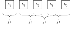
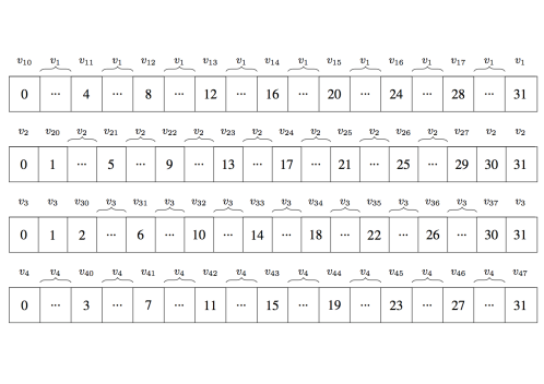
Figure 5: Features $F$ (left) and $F^{\prime}$ (right).

Because of space restriction we have omitted the computations, the interested reader can find them in the report version of this paper [21]. At step $3$ one of the possible outcomes of the algorithm based on Shannon is the set of features $S_{1}^{3}=\{f_{1},f_{3},f_{4}\}$, and one of the possible outcomes of the algorithm based on Rényi is $S_{\infty}^{3}=\{f^{\prime}_{1},f^{\prime}_{2},f^{\prime}_{i}\}$ where $i$ can be, equivalently, $3$ or $4$. At this point the method with Shannon can stop, since the residual Shannon entropy of the classification is $H_{1}(C\mid S_{1}^{3})=0$, and also the Bayes error is ${\cal B}(C\mid S_{1}^{3})=0$, which is the optimal situation in the sense that the classification is completely accurate. $S_{\infty}^{3}$ on the contrary does not contain enough features to give a completely accurate classification, for that we have to make a further step. We can see that $S_{\infty}^{4}=F^{\prime}$, and finally we have $H_{\infty}(C\mid S_{\infty}^{4})=0$.

Thus in this particular example we have that for small values of the threshold on the accuracy our method gives better results. On the other hand, if we want to achieve perfect accuracy (threshold $0$) Shannon gives better results.

5 Evaluation

In this section we evaluate the method for feature selection that we have proposed, and we compare it with the one based on Shannon entropy by [5] and [29].

To evaluate the effect of feature selection, some classification methods have to be trained and tested on the selected data. We used two different methods to avoid the dependency of the result on a particular algorithm. We chose two widely used classifiers: the Support Vector Machines (SVM) and the Artificial Neural Networks (ANN).

Even though the two methods are very different, they have in common that their efficiency is highly dependent on the choice of certain parameters. Therefore, it is worth spending some effort to identify the best values. Furthermore, we should take into account that the particular paradigm of SVM we chose only needs 2 parameters to be set, while for ANN the number of parameters increases (at least 4).

It is very important to choose values as robust as possible for the parameters. It goes without saying that the strategy used to pick the best parameter setting should be the same for both Shannon entropy and Rényi min-entropy. On the other hand for SVM and ANN we used two different hyper-parameter tuning algorithms, given that the number and the nature of the parameters to be tuned for those classifiers is different.

In the case of SVM we tuned the cost parameter of the objective function for margin maximization (C-SVM) and the parameter which models the shape of the RBF kernel’s bell curve ($\gamma$). Grid-search and Random-search are quite time demanding algorithms for the hyper-parameter tuning task but they’re also widely used and referenced in literature when it comes to SVM. Following the guidelines in [8] and [22], we decided to use Grid-search, which is quite suitable when we have to deal with only two parameters. In particular we performed Grid-search including a 10 folds CV step.

Things are different with ANN because many more parameters are involved and some of them change the topology of the network itself. Among the various strategies to attack this problem we picked Bayesian Optimization [28]. This algorithm combines steps of extensive search for a limited number of settings before inferring via Gaussian Processes (GP) which is the best setting to try next (with respect to the mean and variance and compared to the best result obtained in the last iteration of the algorithm). In particular we tried to fit the best model by optimizing the following parameters:

• number of hidden layers

• number of hidden neurons in each layer

• learning rate for the gradient descent algorithm

• size of batches to update the weight on network connections

• number of learning epochs

To this purpose, we included in the pipeline of our code the Spearmint Bayesian optimization codebase. Spearmint, whose theoretical bases are explained in [28], calls repeatedly an objective function to be optimized. In our case the objective function contained some tensorflow machine learning code which run a 10 folds CV over a dataset and the objective was to maximize the accuracy of validation. The idea was to obtain a model able to generalize as much as possible using only the selected features before testing on a dataset which had never been seen before.

We had to decide the stopping criterion, which is not provided by Spearmint itself. For the sake of simplicity we decided to run it for a time lapse which has empirically been proven to be sufficient in order to obtain results meaningful for comparison. A possible improvement would be to keep running the same test (with the same number of features) for a certain amount of time without resetting the computation history of the package and only stop testing a particular configuration if the same results is output as the best for $k$ iterations in a row (for a given $k$).

Another factor, not directly connected to the different performances obtained with different entropies, but which is important for the optimization of ANN, is the choice of the activation functions for the layers of neurons. In our work we have used ReLU for all layers because it is well known that it works well for this aim, it is easy to compute (the only operation involved is the max) and it avoids the sigmoid saturation issue.

5.1 Experiments

As already stated, at the $i$-th step of the feature selection algorithm we consider all the features which have already been selected in the previous $i-1$ step(s). For the sake of limiting the execution time, we decided to consider only the first 50 selected features with both metrics. We tried our pipeline on the following datasets:

• BASEHOCK dataset: 1993 instances, 4862 features, 2 classes. This dataset has been obtained from the 20 newsgroup original dataset.

• SEMEION dataset: 1593 instances, 256 features, 10 classes. This is a dataset with encoding of hand written characters.

• GISETTE dataset: 6000 instances, 5000 features, 2 classes. This is the discretized version of the NIPS 2003 dataset which can be downloaded from the site of Professor Gavin Brown, Manchester University.

We implemented a bootstrap procedure (5 iterations on each dataset) to shuffle data and make sure that the results do not depend on the particular split between training, validation and test set. Each one of the 5 bootstrap iterations is a new and unrelated experimental run. For each one of them a different training-test sets split was taken into account. Features were selected analyzing the training set (the test set has never been taken into account for this part of the work). After the feature selection was executed according to both Shannon and Rényi min-entropy, we considered all the selected features adding one at each time. So, for each bootstrap iteration we had 50 steps, and in each step we added one of the selected features, we performed hyper-parameter tuning with 10 folds CV, we trained the model with the best parameters on the whole training set and we tested it on the test set (which the model had never seen so far). This procedure was performed both for SVM and ANN.

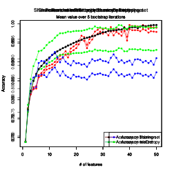
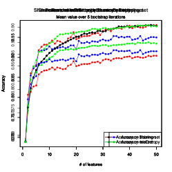
Figure 6: Accuracy of the ANN and SVM classifiers on the BASEHOCK dataset

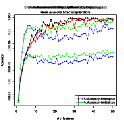
Figure 7: Accuracy of the ANN and SVM classifiers on the GISETTE dataset

We computed the average performances over the 5 iterations and the results are in Figures 6, 7, and 8. In all cases the feature selection method using Rényi min-entropy usually gave better results than Shannon, especially with the BASEHOCK dataset.

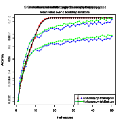
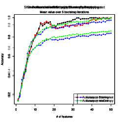
Figure 8: Accuracy of the ANN and SVM classifiers on the SEMEION dataset

6 Related works

In the last two decades, due to the growing interest for machine learning, much research effort has been devoted to the feature reduction problem, and several methods have been proposed. In this section we discuss those closely related to our work, namely those which are based on information theory. For a more complete overview we refer to [4], [29] and [5].

The approach most related to our proposal is that of [5] and [29], which differ from ours in that it uses Shannon entropy instead than Rényi min entropy. We have discussed and compared their method with ours in the technical body of this paper.

As far as we know, in the context of feature selection Rényi min-entropy has only been considered by [13] (although in the experiments they only show results for other Rényi entropies). The notion of conditional Rényi min-entropy they use, however, is that of [6], which formalizes it along the lines of conditional Shannon entropy. Namely, the conditional min-entropy of $X$ given $Y$ is defined in [6] as the expected value of the entropy of $X$ for each given value of $Y$. Such definition, however, violates the monotonicity principle: knowing the value of $Y$ may increase the entropy of $X$ instead of decreasing it. It is clear, therefore, that basing a method on this notion of entropy could lead to strange results.

Two key concepts that have been widely used are relevance and redundancy. Relevance refers to the importance for the classification of the feature under consideration at time $t$, $f^{t}$, and it is in general modeled as $I(C;f^{t})$, where $I$ is the Shannon mutual information. Redundancy represents how much the information of $f^{t}$ is already covered by $S$, and it is often modeled as $I(S;f\textsuperscript{t})$. In general, we want to maximize relevance and minimize redundancy.

One of the first algorithms ever implemented was the MIFS algorithm proposed by [3], based on a greedy strategy. At the first step it selects $f\textsuperscript{1}=\operatorname*{{\rm argmax}}_{f_{i}\in F}I(C;f_{i})$, and at step $t$ it selects $f\textsuperscript{t}=\operatorname*{{\rm argmax}}_{f_{i}\in F\setminus S\textsuperscript{t-1}}[I(C;f_{i})-\beta\sum_{f_{s}\in S\textsuperscript{t-1}}I(f_{s};f_{i})]$ where $\beta$ is a parameter that controls the weight of the redundancy part.

The mRMR approach (redundancy minimization and relevance maximization) proposed by [23] is based on the same strategy as MIFS. However the redundancy term is now substituted by its mean over the elements of the subset $S$ so to avoid its value to grow when new attributes are selected.

A common issue with these two methods is that they do not take into account the conditional mutual information $I(C;f\textsuperscript{t}\mid S)$ for the choice of the next feature to be selected. As a consequence, it may happen that a feature $f\textsuperscript{t}$ has a high correlation with some other feature in the set $S$ of features already chosen, but, if $I(C;f\textsuperscript{t})$ is high, $f\textsuperscript{t}$ may still be selected despite the fact that it is highly redundant.

More recent algorithms involve the ideas of joint mutual entropy $I(C;f_{i},S)$ (JMI, [4]) and conditional mutual entropy $I(C;f_{i}\mid S)$ (CMI, [14]). The step for choosing the next feature with JMI is $f\textsuperscript{t}=\operatorname*{{\rm argmax}}_{f_{i}\in F\setminus S\textsuperscript{t-1}}\big{\{}min_{f_{s}\in S\textsuperscript{t-1}}I(C;f_{i},f_{s})\big{\}}$, while with CMI is $f\textsuperscript{t}=\operatorname*{{\rm argmax}}_{f_{i}\in F\setminus S\textsuperscript{t-1}}\big{\{}min_{f_{s}\in S\textsuperscript{t-1}}I(C;f_{i}\mid f_{s})\big{\}}$. In both cases the already selected features are taken into account one by one when compared to the new feature $f\textsuperscript{t}$. In [30] the following correlation between JMI and CMI was proved:

$$I(C;f_{i},S)=H(C)-H(C\mid S)+H(C\mid S)-H(C\mid S)=I(C;S)+I(C;f_{i}\mid S).$$

7 Conclusion and Future Work

We have proposed a method for feature selection based on a notion of conditional Rényi min-entropy. Although our method is in general incomparable with the corresponding one based on Shannon entropy, in the experiments we performed it turned out that our methods always achieved better results.

As future work, we plan to compare our proposal with other information-theoretic methods for feature selection. In particular, we plan to investigate the application of other notions of entropy which are the state-of-the-art in security and privacy, like the notion of $g$-vulnerability [1], which seems promising for its flexibility and capability to represent a large spectrum of possible classification strategies.

References

- [1] Alvim, M.S., Chatzikokolakis, K., Palamidessi, C., Smith, G.: Measuring information leakage using generalized gain functions. In: Proc. of CSF. pp. 265–279 (2012)
- [2] Arimoto, S.: Information measures and capacity of order for discrete memoryless channels. In: Topics in Information Theory, Proc. Coll. Math. Soc. Janos Bolyai. pp. 41–52 (1975)
- [3] Battiti, R.: Using mutual information for selecting features in supervised neural net learning. IEEE Trans. Neural Networks 5(4), 537–550 (1994)
- [4] Bennasar, M., Hicks, Y., Setchi, R.: Feature selection using joint mutual information maximisation. Expert Syst. Appl 42(22), 8520–8532 (2015)
- [5] Brown, G., Pocock, A.C., Zhao, M.J., Luján, M.: Conditional likelihood maximisation: A unifying framework for information theoretic feature selection. JMLR 13, 27–66 (2012)
- [6] Cachin, C.: Entropy Measures and Unconditional Security in Cryptography. Ph.D. thesis, ETH (1997)
- [7] Cai, J., Luo, J., Wang, S., Yang, S.: Feature selection in machine learning: A new perspective. Neurocomputing 300, 70 – 79 (2018)
- [8] Chang, C.C., Lin, C.J.: LIBSVM: A library for support vector machines. ACM Trans. on Intelligent Systems and Technology 2, 27:1–27:27 (2011), software available at http://www.csie.ntu.edu.tw/~cjlin/libsvm
- [9] Cover, T.M., Thomas, J.A.: Elements of Information Theory. J. Wiley & Sons, Inc. (1991)
- [10] Csiszár, I.: Generalized cutoff rates and Rényi’s information measures. Trans. on Information Theory 41(1), 26–34 (1995)
- [11] Davies, S., Russell, S.: Np-completeness of searches for smallest possible feature sets (1994)
- [12] Einicke, G.A., Sabti, H.A., Thiel, D.V., Fernandez, M.: Maximum-entropy-rate selection of features for classifying changes in knee and ankle dynamics during running. IEEE Journal of Biomedical and Health Informatics 22(4), 1097–1103 (2018)
- [13] Endo, T., Kudo, M.: Weighted Naïve Bayes Classifiers by Renyi Entropy. In: Proc. of CIARP. LNCS, vol. 8258, pp. 149–156. Springer (2013)
- [14] Fleuret, F.: Fast binary feature selection with conditional mutual information. JMLR 5, 1531–1555 (2004)
- [15] Guyon, I., Elisseeff, A.: An introduction to variable and feature selection. JMLR 3, 1157–1182 (2003)
- [16] Jain, A.K., Duin, R.P.W., Mao, J.: Statistical pattern recognition: A review. IEEE Trans. on Pattern Analysis and Machine Intelligence 22(1), 4–37 (2000)
- [17] Karp, R.M.: Reducibility among Combinatorial Problems, pp. 85–103. Springer US (1972)
- [18] Liu, H., Yu, L.: Toward integrating feature selection algorithms for classification and clustering. IEEE Trans. on Knowledge and Data Engineering 17(4), 491–502 (2005)
- [19] Liu, J., Lin, Y., Wu, S., Wang, C.: Online multi-label group feature selection. Knowledge-Based Systems 143, 42 – 57 (2018)
- [20] Nakariyakul, S.: High-dimensional hybrid feature selection using interaction information-guided search. Knowledge-Based Systems 145, 59 – 66 (2018)
- [21] Palamidessi, C., Romanelli, M.: Feature selection with rényi min-entropy. Tech. rep., INRIA (2018), available at https://hal.archives-ouvertes.fr/hal-01830177
- [22] Pedregosa, F.e.a.: Scikit-learn: Machine learning in Python. JMLR 12, 2825–2830 (2011)
- [23] Peng, H., Long, F., Ding, C.H.Q.: Feature selection based on mutual information: Criteria of max-dependency, max-relevance, and min-redundancy. IEEE Trans. Pattern Anal. Mach. Intell 27(8), 1226–1238 (2005)
- [24] Rényi, A.: On Measures of Entropy and Information. In: Proceedings of the 4th Berkeley Symposium on Mathematics, Statistics, and Probability. pp. 547–561 (1961)
- [25] Sheikhpour, R., Sarram, M.A., Gharaghani, S., Chahooki, M.A.Z.: A survey on semi-supervised feature selection methods. Pattern Recognition 64, 141 – 158 (2017)
- [26] Sibson, R.: Information radius. Z. Wahrscheinlichkeitsth. und Verw. Geb 14, 149–161 (1969)
- [27] Smith, G.: On the foundations of quantitative information flow. In: Proc. of FOSSACS. LNCS, vol. 5504, pp. 288–302. Springer (2009)
- [28] Snoek, J., Larochelle, H., Adams, R.P.: Practical bayesian optimization of machine learning algorithms. In: Proc. of NIPS 2012. pp. 2960–2968 (2012)
- [29] Vergara, J.R., Estévez, P.A.: A review of feature selection methods based on mutual information. Neural Computing and Applications 24(1), 175–186 (2014)
- [30] Yang, H.H., Moody, J.: Feature selection based on joint mutual information. In: In Proceedings of Int. ICSC Symposium on Advances in Intelligent Data Analysis. pp. 22–25 (1999)