A domain decomposition method for Isogeometric multi-patch problems with inexact local solvers

Abstract

In Isogeometric Analysis, the computational domain is often described as multi-patch, where each patch is given by a tensor product spline/NURBS parametrization. In this work we propose a FETI-like solver where local inexact solvers exploit the tensor product structure at the patch level. To this purpose, we extend to the isogeometric framework the so-called All-Floating variant of FETI, that allows us to use the Fast Diagonalization method at the patch level. We construct then a preconditioner for the whole system and prove its robustness with respect to the local mesh-size $h$ and patch-size $H$ (i.e., we have scalability). Our numerical tests confirm the theory and also show a favourable dependence of the computational cost of the method from the spline degree $p$. Keywords: Isogeometric Analysis, domain decomposition, FETI, IETI, preconditioners, Fast Diagonalization.

1 Introduction

Isogeometric Analysis (IgA) was introduced in the seminal paper [19] as an extension of finite element analysis. The key idea is to use the same basis functions that describe the computational domain, typically B-splines, NURBS or extensions, also to represent the unknown solution of the partial differential equations.

In this work, we are concerned with the numerical solution of large isogeometric compressible linear elasticity problems in multi-patch domains, that is, domains defined as the union of several patches, each described by a different tensor product spline/NURBS parametrization (see [8]). Knowing the advantages that come from the use of high-degree and high-continuity spline approximation (see for example [13, 1, 32, 36, 5, 34]), we are particularly interested in this case. It is also known that the development of linear solvers, both direct and iterative, for high-degree splines is a challenging task, see [7, 6].

Our starting point is [33], where it has been shown the potential of the Fast Diagonalization (FD) method to construct fast solvers for elliptic isogeometric problems. The FD method is a direct solver introduced in [22], that can be applied to problems with a Sylvester-like structure. In general, elliptic isogeometric problems do not possess the required Sylvester-like structure, even on a single patch, unless the patch parametrization is trivial. However, [33] constructs efficient preconditioners (that is, inexact solvers) with the required structure on a single patch. Similarly, here we use FD as an inexact and fast solver for problems at the patch level.

Our approach is based on the Finite Element Tearing and Interconnecting (FETI) idea, that, after its appearance in  [15], has been widely developed and adopted in finite element solvers, see [37]. IETI, the isogeometric version of FETI, has been introduced in [21]. In particular, we develop in this paper an All-Floating IETI (in short AF-IETI) method, the isogeometric version of the All-Floating FETI introduced in [27], which is in turn similar to the so-called total-FETI of [12]. With this variant of FETI, both the global continuity of the solution and the Dirichlet boundary conditions are weakly imposed by Lagrange multipliers. The choice of the AF-IETI formulation is crucial for us since it yields the Sylvester-like structure that we need to use FD as inexact local solver. To allow inexact solvers, a saddle point formulation as in [20] is also required.

To show the potential of the proposed inexact AF-IETI, we compare numerically its performance to AF-IETI with the exact local solvers. Our results indicate that the inexact approach requires orders of magnitude less time than the exact one. Moreover, and perhaps even more important, numerical tests indicate that the performance of the preconditioner does not deteriorate as the degree $p$ is increased.

Domain decomposition methods represent an active research area in isogeometric analysis. We recall the overlapping Schwarz methods studied in [4, 2], the BDDC methods with related preconditioners studied from [3], the dual-primal approach introduced in [21] and further studied in [17, 28]. Domain decomposition approaches with inexact local solvers have been studied in [18, 35]. The case of trimmed domains has ben recently addressed in [10]

The paper is organized as follows. In Section 2 we present the basics of multi-patch based IgA and in Section 3 we introduce the model problem as well as its discrete formulation. The AF-IETI method is described in Section 4, while exact and inexact local solvers are introduced and analyzed in Section 5. Numerical results are reported in Section 6 and, finally, Section 7 contains some conclusions and future directions of research.

2 Preliminaries

2.1 B-splines

Given two integers $m,p>0$, we introduce a knot vector $\Xi:=\{0=\xi_{1}\leq\dotsc\leq\xi_{m+p+1}=1\}$ in the interval $[0,1]$, where $m$ and $p$ are, respectively, the number of basis functions that will be built from the knot vector and their polynomial degree. We consider open knot vectors, i.e. we set $\xi_{1}=\dotsc=\xi_{p+1}=0$ and $\xi_{m+1}=\dotsc=\xi_{m+p+1}=1$. Following Cox-de Boor recursion formulas [9], univariate B-splines are piecewise polynomials defined for $i=1,\dots,m$ as follows:

for $p=0$

$$\widehat{b}_{i,0}(\eta)=\begin{cases}1&{\textrm{if }}\xi_{i}\leq\eta<\xi_{i+1},\\ 0&\textrm{otherwise},\end{cases}$$

for $p\geq 1$

$$\widehat{b}_{i,p}(\eta)=\!\begin{cases}\dfrac{\eta-\xi_{i}}{\xi_{i+p}-\xi_{i}}\widehat{b}_{i,p-1}(\eta)+\dfrac{\xi_{i+p+1}-\eta}{\xi_{i+p+1}-\xi_{i+1}}\widehat{b}_{i+1,p-1}(\eta)&{\textrm{if }}\xi_{i}\leq\eta<\xi_{i+p+1},\\[8.0pt] 0&\textrm{otherwise,}\end{cases}$$

where we adopted the convention $\frac{0}{0}=0$. The multiplicity of the internal knots influences the smoothness of the B-splines (see [8]). The corresponding univariate spline space is defined as

$$\widehat{\mathcal{S}}_{p}:=\mathrm{span}\{\widehat{b}_{i,p}\}_{i=1}^{m}.$$

We also introduce the mesh-size $h:=\max\{\xi_{i+1}-\xi_{i}\ |\ i=1,\dots,m+p\}$. We remark that the first and last basis function are nodal at the endpoint of the unit interval, i.e. $\widehat{b}_{1,p}\left(0\right)=\widehat{b}_{m,p}\left(1\right)=1$.

We consider multivariate B-splines as tensor products of univariate ones. In particular, for $d$-dimensional problems, given $2d$ integers $m_{l},p_{l}>0$ for $l=1,\dots,d,$ we introduce $d$ univariate knot vectors $\Xi_{l}:=\{\xi_{l,1},\dots,\xi_{l,m_{l}+p_{l}+1}\}$ for $l=1,..,d$ and the corresponding mesh-sizes denoted with $h_{l}$ for $l=1,..,d$. For simplicity we suppose that the degree of the B-splines is the same in all parametric direction, i.e. we set $p_{1}=\dots=p_{d}=:p$, but the general case is similar. For a multi-index $\boldsymbol{i}=(i_{1},\dotsc,i_{d})$, we define the multivariate B-spline as follows

$$\widehat{B}_{\boldsymbol{i},{p}}(\boldsymbol{\eta}):=\widehat{b}_{i_{1},p}(\eta_{1})\dotsc\widehat{b}_{i_{d},p}(\eta_{d})$$

where $\boldsymbol{\eta}=(\eta_{1},\dotsc,\eta_{d})$. Hence, the multivariate spline space on the parametric domain $\widehat{\Omega}:=\left[0,1\right]^{d}$ is defined as

$$\boldsymbol{\widehat{\mathcal{S}}}_{{p}}:=\underbrace{\widehat{\mathcal{S}}_{p}\times\dots\times\widehat{\mathcal{S}}_{p}}_{d}=\mathrm{span}\{\widehat{B}_{\boldsymbol{i},{p}}\ |\ i_{l}=1,\dotsc,m_{l};l=1,\dotsc,d\}.$$

We also introduce the global mesh-size, defined as $h:=\max\{h_{l}\ |\ l=1,\dots,d\}$.

2.2 Multi-patch domains

Let $\Omega\subset\mathbb{R}^{d}$ be the union of $\mathcal{N}_{patch}$ isogeometric patches, i.e $\overline{\Omega}=\bigcup_{k=1}^{\mathcal{N}_{patch}}\overline{\Omega}^{(k)}$ and $\Omega^{(j)}\cap\Omega^{(k)}=\emptyset$ for $j\neq k$. In the present approach, these patches coincide with the non-overlapping subdomains whose prescription is the starting point of every FETI method. Let $H^{(k)}$ be the diameter of $\Omega^{(k)}$ for $k=1,\dots,\mathcal{N}_{patch}$ and $H:=\max\{H^{(k)}\ |\ k=1,\dots,\mathcal{N}_{patch}\}$. For each patch, given $d+1$ integers $m_{1}^{(k)},\dots,m_{d}^{(k)},p^{(k)}>0$, we introduce open knot vectors $\Xi_{l}^{(k)}:=\{0=\xi^{(k)}_{1}\leq\dotsc\leq\xi^{(k)}_{m^{(k)}_{l}+p^{(k)}+1}=1\}$ for $l=1,\dots,d$ and the local mesh-size $h^{(k)}$. For simplicity, we suppose that the degree of the B-splines is the same in each patch, i.e. we set $p^{(1)}=\dots=p^{(\mathcal{N}_{patch})}=:p$, even if the general case is similar. Let also $h:=\max\{h^{(k)}\ |\ k=1,\dots,\mathcal{N}_{patch}\}$. We will make the following assumption on the quasi-regularity of the meshes and on the diameter of the patches.

Assumption 1.

There exists $\alpha\in(0,1]$, independent of $h^{(k)}$ and $H^{(k)}$ for $k=1,\dots,\mathcal{N}_{patch}$, such that each non-empty knot span $(\xi^{(k)}_{l,i},\xi^{(k)}_{l,i+1})$ fulfils $\alpha h^{(k)}\leq\xi_{l,i+1}^{(k)}-\xi_{l,i}^{(k)}\leq h^{(k)}$ for $i=1,\dots m^{(k)}_{l}+p$, for $l=1,\dots d$ and for $k=1,\dots,\mathcal{N}_{patch}$ and each $H^{(k)}$ fulfils $\alpha H\leq H^{(k)}\leq H$ for $k=1,\dots,\mathcal{N}_{patch}$.

We denote the multivariate spline-space associated as $\boldsymbol{\widehat{\mathcal{S}}}^{(k)}_{{p}}:=\mathrm{span}\{\widehat{B}^{(k)}_{\boldsymbol{i},{p}}\ |\ i_{l}=1,\dotsc,m^{(k)}_{l};l=1,\dotsc,d\}$. By introducing a colexicographical reordering of the basis functions, we have

$$\boldsymbol{\widehat{\mathcal{S}}}^{(k)}_{p}:=\mathrm{span}\left\{\widehat{B}^{(k)}_{{i},p}\ |\ i=1,\dots,n^{(k)}\right\},$$

where $n^{(k)}:=\mathrm{dim}(\boldsymbol{\widehat{\mathcal{S}}}^{(k)}_{p})$. Each $\Omega^{(k)}$ is represented by a non-singular spline parametrization $\mathcal{F}^{(k)}\in\left[\boldsymbol{\widehat{\mathcal{S}}}^{(k)}_{p}\right]^{d}$, i.e. $\Omega^{(k)}=\mathcal{F}^{(k)}(\widehat{\Omega})$ and the Jacobian matrix $J_{\mathcal{F}^{(k)}}$ is invertible everywhere. According to the isoparametric concept, the isogeometric space on each patch is defined as

$$V^{(k)}_{h}:=\mathrm{span}\left\{{B}_{{i},p}^{(k)}:=\widehat{B}^{(k)}_{{i},p}\circ\left(\mathcal{F}^{(k)}\right)^{-1}\ \bigg{|}\ i=1,\dotsc,n^{(k)}\right\},$$ (2.1)

while the isogeometric space over $\Omega$ is defined as

$$V_{h}:=\Pi_{k=1}^{\mathcal{N}_{patch}}V_{h}^{(k)}=\left\{v\in L^{2}(\Omega)\ \bigg{|}\ v_{|_{\Omega^{(k)}}}\in V_{h}^{(k)},\ k=1,\dots,\mathcal{N}_{patch}\right\}.$$

Note that functions in $V_{h}$ are not necessarily continuous.

Through this paper, we consider both conforming and non-conforming meshes at the patch interfaces. In the first case, for all $j$ and $k$ s.t. $\partial\Omega^{(k)}\cap\partial\Omega^{(j)}\neq\emptyset$ and this intersection is not a point, $\Omega^{(k)}$ and $\Omega^{(j)}$ are fully matching (see [19]). In the second case, we allow that on a given interface the knot vector of one patch can be more refined than the knot vector of an adjacent patch (see Figure 1a in Section 6). With this assumption, we have that splines of the coarser side can be written as a linear combination of splines of the finer one.

3 Model problem and its discretization

Let $\Omega\subset\mathbb{R}^{d}$ be a computational domain described by a multi-patch spline parametrization, as in Section 2.2, and let $\partial\Omega$ denote its boundary. Suppose that $\partial\Omega=\partial\Omega_{D}\cup\partial\Omega_{N}$ with $\partial\Omega_{D}\cap\partial\Omega_{N}=\emptyset$, where $\partial\Omega_{D}$ has positive measure. Let $\boldsymbol{f}\in[{L}^{2}(\Omega)]^{d}$, $\ \boldsymbol{g}\in[{L}^{2}(\partial\Omega_{N})]^{d}$ and $H^{1}_{D}(\Omega):=\{v\in H^{1}(\Omega)\ \text{s.t.}\ v=0\text{ on }\partial\Omega_{D}\}$. Then, the variational formulation of the compressible linear elasticity problem we consider reads:

Find $\boldsymbol{u}\in[H^{1}_{D}(\Omega)]^{d}$ s.t. for all $\boldsymbol{v}\in[H^{1}_{D}(\Omega)]^{d}$

$$a(\boldsymbol{u},\boldsymbol{v})=\langle\boldsymbol{F},\boldsymbol{v}\rangle,$$

where we define

$$a(\boldsymbol{u},\boldsymbol{v}):=2\mu\int_{\Omega}\varepsilon(\boldsymbol{u}):\varepsilon(\boldsymbol{v})\ d\boldsymbol{x}+\lambda\int_{\Omega}\left(\nabla\cdot\boldsymbol{u}\right)\left(\nabla\cdot\boldsymbol{v}\right)\ d\boldsymbol{x},\quad\langle\boldsymbol{F},\boldsymbol{v}\rangle:=\int_{\Omega}\boldsymbol{f}\cdot\boldsymbol{v}\ d\boldsymbol{x}+\int_{\partial\Omega_{N}}\boldsymbol{g}\cdot\boldsymbol{v}\ ds$$ (3.1)

and where we used the notation ${\varepsilon}(\boldsymbol{v}):=\frac{1}{2}\left(\nabla\boldsymbol{v}+(\nabla\boldsymbol{v})^{T}\right)$ for the symmetric gradient, while $\lambda$ and $\mu$ denote the material Lamé coefficients.

The corresponding discrete problem we want to solve is then

Find $\boldsymbol{u}_{h}\in[V_{h}\cap H^{1}_{D}(\Omega)]^{d}$ s.t. for all $\boldsymbol{v}_{h}\in[V_{h}\cap H^{1}_{D}(\Omega)]^{d}$

$$a(\boldsymbol{u}_{h},\boldsymbol{v}_{h})=\langle\boldsymbol{F},\boldsymbol{v}_{h}\rangle.$$ (3.2)

4 All-Floating IETI method

In this section, we present the All-Floating IETI (AF-IETI) method, an extension to IgA of the AF-FETI method, introduced in [30], (see also [29]). In this formulation, the FETI interface includes the whole boundary $\partial\Omega$ without distinction between Dirichlet and Neumann boundary.

Let $\Omega$ be the computational domain described as the union of $\mathcal{N}_{patch}$ isogeometric patches $\Omega^{(k)}$ for $k=1,\ldots,\mathcal{N}_{patch}$, as detailed in Section 2.2. We work with the computational spaces

$$\mathcal{V}_{h}^{(k)}:=\left[V_{h}^{(k)}\right]^{d}\quad\text{and}\quad\mathcal{V}_{h}:=\Pi_{k=1}^{\mathcal{N}_{patch}}\mathcal{V}_{h}^{(k)},$$ (4.1)

where $V_{h}^{(k)}$ is defined in (2.1). Note that the space $\mathcal{V}_{h}$ above does not include any boundary condition or continuity condition across the patch boundaries, unlike the space $[V_{h}\cap H^{1}_{D}(\Omega)]^{d}$ used in problem (3.2). Let

$$\mathcal{N}_{dof}^{(k)}:=\mathrm{dim}\left(\mathcal{V}_{h}^{(k)}\right)=\left[n^{(k)}\right]^{d}\quad\text{ and }\quad\mathcal{N}_{dof}:=\mathrm{dim}\left(\mathcal{V}_{h}\right)=\sum_{k=1}^{\mathcal{N}_{patch}}\mathcal{N}_{dof}^{(k)}$$

denote the dimension of the $k-$th local space for $k=1,\ldots,\mathcal{N}_{patch}$, and the dimension of the whole space, respectively. Each function $\boldsymbol{v}^{(k)}_{h}\in\mathcal{V}_{h}^{(k)}$ is uniquely represented by a coordinate vector $\mathbf{v}^{(k)}\in\mathbb{R}^{\mathcal{N}^{(k)}_{dof}}$. Similarly, each function $\boldsymbol{v}_{h}\in\mathcal{V}_{h}$ is associated to a coordinate vector $\mathbf{v}\in\mathbb{R}^{\mathcal{N}_{dof}}$ of the form

$$\mathbf{v}:=\begin{bmatrix}\mathbf{v}^{(1)}\\ \vdots\\ \mathbf{v}^{(\mathcal{N}_{patch})}\end{bmatrix}.$$

We assemble the local stiffness matrices $\mathbf{A}^{(k)}$ and local right-hand-side vectors $\mathbf{f}^{(k)}$ by integrating the appropriate expressions over individual patches $\Omega^{(k)}$ for $k=1,\dots,\mathcal{N}_{patch}$. The matrices $\mathbf{A}^{(k)}$ for $k=1,\dots,\mathcal{N}_{patch}$ are symmetric, positive semidefinite and singular. We then define the block-diagonal matrix $\mathbf{A}$ and the load vector $\mathbf{f}$ as

$$\mathbf{A}:=\begin{bmatrix}\mathbf{A}^{(1)}&&\\ &\ddots&\\ &&\mathbf{A}^{(\mathcal{N}_{patch})}\end{bmatrix}\in\mathbb{R}^{\mathcal{N}_{dof}\times\mathcal{N}_{dof}}\quad\text{and}\quad\mathbf{f}:=\begin{bmatrix}\mathbf{f}^{(1)}\\ \vdots\\ \mathbf{f}^{(\mathcal{N}_{patch})}\end{bmatrix}\in\mathbb{R}^{\mathcal{N}_{dof}}$$ (4.2)

where each local matrix $\mathbf{A}^{(k)}$ has a natural block structure, that follows from the vectorial nature of the space $\mathcal{V}_{h}^{(k)}$ in (4.1) and of the bilinear form $a(\cdot,\cdot)$ in (3.1):

$$\mathbf{A}^{(k)}:=\begin{bmatrix}\mathbf{A}^{(k)}_{1,1}&\dots&\mathbf{A}^{(k)}_{1,d}\\ \vdots&\ddots&\vdots\\ \mathbf{A}^{(k)}_{d,1}&\dots&\mathbf{A}^{(k)}_{d,d}\end{bmatrix}.$$ (4.3)

The interface $\Gamma$ is defined as the union of the local interfaces, that in our method are the whole local boundaries $\partial\Omega^{(k)}$, as

$$\Gamma:=\bigcup_{k=1}^{\mathcal{N}_{patch}}\partial\Omega^{(k)}.$$

Note that, thanks to the use of open knot vectors, we can identify the local degrees-of-freedom associated to basis functions that have non-zero support on the local interface $\partial\Omega^{(k)}$ and the remaining degrees-of-freedom, that are associated to the interior functions. Thus, we also assume a partition of each local matrix $\mathbf{A}^{(k)}$ as

$$\mathbf{A}^{(k)}:=\begin{bmatrix}\mathbf{A}^{(k)}_{II}&\mathbf{A}^{(k)}_{I\Gamma}\\ \mathbf{A}^{(k)}_{\Gamma I}&\mathbf{A}^{(k)}_{\Gamma\Gamma}\end{bmatrix},$$ (4.4)

where the subscript $\Gamma$ refers to the interface degrees-of-freedom that belongs to the $k$-th patch, while $I$ indicates the remaining local interior degrees-of-freedom. Let also $\mathcal{N}_{\Gamma}^{(k)}$ be the dimension of $\mathbf{A}^{(k)}_{\Gamma\Gamma}$ for $k=1,\dots,\mathcal{N}_{patch}$, i.e. $\mathbf{A}^{(k)}_{\Gamma\Gamma}\in\mathbb{R}^{\mathcal{N}_{\Gamma}^{(k)}\times\mathcal{N}_{\Gamma}^{(k)}}$ for $k=1,\dots,\mathcal{N}_{patch}$.

As the functions in $\mathcal{V}_{h}$ are in general discontinuous across the patch boundaries and do not have prescribed Dirichlet boundary conditions, we need to impose these constraints separately. To this end, we introduce the sparse matrix $\mathbf{B}\in\mathbb{R}^{\mathcal{N}_{c}\times\mathcal{N}_{dof}}$, where $\mathcal{N}_{c}$ denotes the number of conditions to impose. In particular, $\mathbf{B}\mathbf{v}=\mathbf{0}$ when the function $\boldsymbol{v}_{h}\in\mathcal{V}_{h}$ corresponding to the vector $\mathbf{v}\in\mathbb{R}^{\mathcal{N}_{dof}}$ satisfies homogeneous Dirichlet boundary conditions and it is continuous across the patches. If Dirichlet boundary conditions are non-homogeneous, then also the right-hand side has to be modified (see [12] for further details). Without loss of generality, we assume that $\mathrm{ker}(\mathbf{B}^{T})=\boldsymbol{0}$, i.e. there are no redundant constraints and $\mathrm{range}(\mathbf{B})=\mathbb{R}^{\mathcal{N}_{c}}$.

By introducing a vector of Lagrange multipliers $\boldsymbol{\lambda}\in\mathbb{R}^{\mathcal{N}_{c}}$, problem (3.2) can be reformulated as follows:

Find $(\mathbf{u},\boldsymbol{\lambda})\in\mathbb{R}^{\mathcal{N}_{dof}}\times\mathbb{R}^{\mathcal{N}_{c}}$ such that

$$\begin{bmatrix}\mathbf{A}&\mathbf{B}^{T}\\ \mathbf{B}&\mathbf{0}\end{bmatrix}\begin{bmatrix}\mathbf{u}\\ \boldsymbol{\lambda}\end{bmatrix}=\begin{bmatrix}\mathbf{f}\\ \mathbf{0}\end{bmatrix}.$$ (4.5)

The difficulty in preconditioning (4.5) is that $\mathbf{A}$ is singular. Following [20], we introduce the matrix

$$\mathbf{R}:=\begin{bmatrix}\mathbf{R}^{(1)}&&\\ &\ddots&\\ &&\mathbf{R}^{(\mathcal{N}_{patch})}\end{bmatrix},$$

where the matrices $\mathbf{R}^{(k)}$ are defined such that $\mathrm{range}(\mathbf{R}^{(k)})=\mathrm{ker}(\mathbf{A}^{(k)})$ for $k=1,\ldots\mathcal{N}_{patch}$. Thus, we also have that $\mathrm{range}(\mathbf{R})=\mathrm{ker}(\mathbf{A})$. In our case, $\mathbf{R}^{(k)}$ represents the space of rigid body motions on the patch $\Omega^{(k)}$. For three-dimensional problems, the case addressed in the numerical experiments of this paper, this space is spanned by three translations and three infinitesimal rotations

$$\boldsymbol{r}_{1}:=\begin{bmatrix}1\\ 0\\ 0\end{bmatrix} \boldsymbol{r}_{2}:=\begin{bmatrix}0\\ 1\\ 0\end{bmatrix},\quad\boldsymbol{r}_{3}:=\begin{bmatrix}0\\ 0\\ 1\end{bmatrix},\quad\boldsymbol{r}_{4}:=\begin{bmatrix}0\\ \boldsymbol{x}_{3}\\ -\boldsymbol{x}_{2}\end{bmatrix} \boldsymbol{r}_{5}:=\begin{bmatrix}\boldsymbol{x}_{3}\\ 0\\ -\boldsymbol{x}_{1}\end{bmatrix},\quad\boldsymbol{r}_{6}:=\begin{bmatrix}\boldsymbol{x}_{2}\\ -\boldsymbol{x}_{1}\\ 0\end{bmatrix}.$$ , ,

Note that $\mathrm{ker}(\mathbf{A})\cap\mathrm{ker}(\mathbf{B})=\boldsymbol{0}$, hence system (4.5) is uniquely solvable.

Multiplying the first block of equations of (4.5) by $\mathbf{R}^{T}$ and using that $\mathbf{R}^{T}\mathbf{A}=\mathbf{0}$, we get

$$\mathbf{R}^{T}\mathbf{B}^{T}\boldsymbol{\lambda}=\mathbf{R}^{T}\mathbf{f}.$$

Let $\mathbf{G}:=\mathbf{B}\mathbf{R}$ and decompose $\boldsymbol{\lambda}=\boldsymbol{\lambda}_{0}+\boldsymbol{\chi}$ such that $\boldsymbol{\lambda}_{0}$ satisfies

$$\mathbf{G}^{T}\boldsymbol{\lambda}_{0}=\mathbf{R}^{T}\mathbf{f},$$

and $\boldsymbol{\chi}\in\mbox{ker}(\mathbf{G}^{T})$. We introduce the orthogonal projection onto $\mbox{ker}(\mathbf{G}^{T})$

$$\mathcal{P}_{{\chi}}:=\mathbf{I}_{\mathcal{N}_{c}}-\mathbf{G}\left(\mathbf{G}^{T}\mathbf{G}\right)^{-1}\mathbf{G}^{T}\in\mathbb{R}^{\mathcal{N}_{c}\times\mathcal{N}_{c}},$$ (4.6)

where $\mathbf{I}_{n}$ denotes the identity matrix of dimension $n\times n$. Finally, the problem we want to solve is the following:

Find $(\mathbf{w},\boldsymbol{\chi})\in\mbox{range}(\mathbf{A})\times\mbox{ker}(\mathbf{G}^{T})$ such that

$$\mathcal{A}\begin{bmatrix}\mathbf{w}\\ \boldsymbol{\chi}\end{bmatrix}:=\begin{bmatrix}\mathbf{A}&(\mathcal{P}_{{\chi}}\mathbf{B})^{T}\\ \mathcal{P}_{{\chi}}\mathbf{B}&\mathbf{0}\end{bmatrix}\begin{bmatrix}\mathbf{w}\\ \boldsymbol{\chi}\end{bmatrix}=\begin{bmatrix}\mathbf{f}-\mathbf{B}^{T}\boldsymbol{\lambda}_{0}\\ \mathbf{0}\end{bmatrix}.$$ (4.7)

We observe that $\mathcal{A}$ is an isomorphism of $\mbox{range}(\mathbf{A})\times\mbox{ker}(\mathbf{G}^{T})$ into itself. Indeed, $\mathbf{A}$ is an isomorphism on $\mbox{range}(\mathbf{A})$, and $(\mathcal{P}_{\chi}\mathbf{B})^{T}\mathbf{v}=\mathbf{B}^{T}\mathcal{P}_{{\chi}}\mathbf{v}=\mathbf{B}^{T}\mathbf{v}$ for every $\mathbf{v}\in\mbox{ker}(\mathbf{G}^{T})$. Thus, system (4.7) is uniquely solvable. Note that, since $\mathcal{P}_{{\chi}}\boldsymbol{\chi}=\boldsymbol{\chi}$ and $\mathcal{P}_{{\chi}}=\mathcal{P}_{{\chi}}^{T}$, the first equation of (4.7) is equivalent to the first equation of  (4.5). However, from the second equation of  (4.7) we see that the solution $\mathbf{w}$ satisfies $\mathcal{P}_{{\chi}}\mathbf{Bw}=\mathbf{0}$ and not $\mathbf{Bw}=\mathbf{0}$.

Thus, given the solution $\begin{bmatrix}\mathbf{w}\\ \boldsymbol{\chi}\end{bmatrix}$ of (4.7), by a straightforword calculation, we can see that the solution $\begin{bmatrix}\mathbf{u}\\ \boldsymbol{\lambda}\end{bmatrix}$ of (4.5) is

$$\mathbf{u}:=\left(\mathbf{I}_{\mathcal{N}_{dof}}-\mathbf{R}\left(\mathbf{G}^{T}\mathbf{G}\right)^{-1}\mathbf{G}^{T}\mathbf{B}\right)\mathbf{w} \boldsymbol{\lambda}:=\boldsymbol{\lambda}_{0}+\boldsymbol{\chi}.$$ ,

Our solver for the linear system (4.7) is MINRES preconditioned by a block-diagonal matrix, whose construction and required properties are discussed below.

Using the splitting of the local matrices into boundary and internal degrees-of-freedom (4.4), we introduce the local Schur complement matrices $\mathbf{S}^{(k)}\in\mathbb{R}^{\mathcal{N}_{\Gamma}^{(k)}\times\mathcal{N}_{\Gamma}^{(k)}}$ for $k=1,\dots,\mathcal{N}_{patch}$, defined as

$$\mathbf{S}^{(k)}:=\mathbf{{A}}^{(k)}_{\Gamma\Gamma}-\mathbf{{A}}^{(k)}_{\Gamma I}\left(\mathbf{{A}}^{(k)}_{II}\right)^{-1}\mathbf{{A}}^{(k)}_{I\Gamma}\quad\text{for }k=1,\cdots,\mathcal{N}_{patch}.$$

Let also $\mathbf{M}^{(k)}\in\mathbb{R}^{\mathcal{N}_{dof}^{(k)}\times\mathcal{N}_{dof}^{(k)}}$ for $k=1,\dots,\mathcal{N}_{patch}$ be the local mass matrices, that are block-diagonal matrices, split component-wise as

$$\mathbf{M}^{(k)}:=\begin{bmatrix}\mathbf{M}^{(k)}_{1}&&\\ &\ddots&\\ &&\mathbf{M}^{(k)}_{d}\end{bmatrix}.$$ (4.8)

We then can build the global Schur complement and mass matrices, as

$$\mathbf{S}:=\begin{bmatrix}\mathbf{S}^{(1)}&&\\ &\ddots&\\ &&\mathbf{S}^{(\mathcal{N}_{patch})}\end{bmatrix}\in\mathbb{R}^{\mathcal{N}_{\Gamma}\times\mathcal{N}_{\Gamma}}\quad\quad\mathbf{M}:=\begin{bmatrix}\mathbf{M}^{(1)}&&\\ &\ddots&\\ &&\mathbf{M}^{(\mathcal{N}_{patch})}\end{bmatrix}\in\mathbb{R}^{\mathcal{N}_{dof}\times\mathcal{N}_{dof}},$$

where $\mathcal{N}_{\Gamma}:=\sum_{k=1}^{\mathcal{N}_{patch}}\mathcal{N}_{\Gamma}^{(k)}$ represents the number of degrees-of-freedom associated to the interface $\Gamma$. Note that $\mathbf{S}$ is the Schur complement of $\mathbf{A}$ that is obtained by eliminating the interior degrees-of-freedom of each patch. We also introduce the scaling diagonal matrix

$$\mathbf{D}_{H}:=\begin{bmatrix}(H^{(1)})^{-2}\ \mathbf{I}_{\mathcal{N}_{dof}^{(1)}}&&\\ &\ddots&\\ &&(H^{(\mathcal{N}_{patch})})^{-2}\ \mathbf{I}_{\mathcal{N}_{dof}^{(\mathcal{N}_{patch})}}\end{bmatrix},$$

and the matrix $\mathbf{B}_{\Gamma}\in\mathbb{R}^{\mathcal{N}_{c}\times\mathcal{N}_{\Gamma}}$ as the restriction of the constraint matrix $\mathbf{B}$ to the interface degrees-of-freedom. Finally, following [20], we define the block-diagonal preconditioner

$$\mathcal{B}^{-1}:=\begin{bmatrix}\mathcal{P}_{{u}}\mathbf{P}_{A}^{-1}\mathcal{P}_{{u}}^{T}&\\ &\mathcal{P}_{{\chi}}\mathbf{P}_{{S}}\mathcal{P}_{{\chi}}^{T}\end{bmatrix},$$ (4.9)

for the system (4.7), where

$$\mathcal{P}_{{u}}:=\mathbf{I}_{\mathcal{N}_{dof}}-\mathbf{R}\left(\mathbf{R}^{T}\mathbf{R}\right)^{-1}\mathbf{R}^{T}$$

is the orthogonal projection onto $\mbox{range}(\mathbf{A})$ and $\mathcal{P}_{\boldsymbol{\chi}}$ is the orthogonal projector onto $\mbox{ker}(\mathbf{G}^{T})$ defined in (4.6). The following general result provides the bound on the condition number for the resulting preconditioned system.

Theorem 1.

Under the assumptions above, given two symmetric matrices $\mathbf{P}_{A}\in\mathbb{R}^{\mathcal{N}_{dof}\times\mathcal{N}_{dof}}$ and $\mathbf{P}_{S}\in\mathbb{R}^{\mathcal{N}_{\Gamma}\times\mathcal{N}_{\Gamma}}$, if there exist positive constants $a_{0},a_{1},s_{0}$ and $s_{1}$ independent of $h$ and $H$ such that

$$a_{0}\,\mathbf{u}^{T}(\mathbf{A}+\mathbf{D}_{H}\mathbf{M})\mathbf{u}\;\leq\;\mathbf{u}^{T}\mathbf{P}_{{A}}\mathbf{u}\;\leq\;a_{1}\,\mathbf{u}^{T}(\mathbf{A}+\mathbf{D}_{H}\mathbf{M})\mathbf{u}\quad\forall\ \mathbf{u}\in\mathrm{range}(\mathbf{A}),$$ (4.10)

$$\\ s_{0}\,\boldsymbol{\lambda}^{T}\mathbf{B}_{\Gamma}\mathbf{S}\mathbf{B}_{\Gamma}^{T}\boldsymbol{\lambda}\;\leq\;\boldsymbol{\lambda}^{T}\mathbf{P}_{S}\boldsymbol{\lambda}\;\leq\;s_{1}\,\boldsymbol{\lambda}^{T}\mathbf{B}_{\Gamma}\mathbf{S}\mathbf{B}_{\Gamma}^{T}\boldsymbol{\lambda}\quad\forall\ \boldsymbol{\lambda}\in\mathrm{ker}(\mathbf{G}^{T}),$$ (4.11)

then the condition number of the system  (4.7) preconditioned by (4.9) fulfils

$$\kappa(\mathcal{B}^{-1}\mathcal{A})\leq C\left(1+\log{\frac{H}{h}}\right)^{2},$$ (4.12)

where $C>0$ is a constant independent of $h$ and $H$.

Proof.

The proof is analogous to the one of [20, Theorem 15], which follows from [20, Lemma 13] and [20, Lemma 14] that can be straightforwardly extended to our framework. We remark that the proof of [20, Lemma 13] uses inverse inequalities and, for that reason, the constant $C$ in (4.12) may depend on the spline degree $p$. ∎

Note in (4.9) the different roles of the matrix $\mathbf{P}_{A}$, that needs to be inverted, and of the matrix $\mathbf{P}_{S}$, that is just multiplied. We further observe that $\mathcal{B}^{-1}$ is an isomorphism of $\mbox{range}(\mathbf{A})\times\mbox{ker}(\mathbf{G}^{T})$ into itself. Hence the preconditioned problem

Find $(\mathbf{w},\boldsymbol{\chi})\in\mbox{range}(\mathbf{A})\times\mbox{ker}(\mathbf{G}^{T})$ such that:

$$\mathcal{B}^{-1}\mathcal{A}\begin{bmatrix}\mathbf{w}\\ \boldsymbol{\chi}\end{bmatrix}=\mathcal{B}^{-1}\begin{bmatrix}\mathbf{f}-\mathbf{B}^{T}\boldsymbol{\lambda}_{0}\\ \mathbf{0}\end{bmatrix}$$

is uniquely solvable and equivalent to (4.7). Finally, the AF-IETI method is the MINRES method applied to the preconditioned system above.

5 Solving the local problems

This section deals with the definition of $\mathbf{P}_{A}$ and $\mathbf{P}_{S}$. These operators are selected block-diagonal, where each block corresponds to a patch. In particular, both the application of $\mathbf{P}_{A}^{-1}$ and the application of $\mathbf{P}_{S}$ correspond to the solution of patch-wise elliptic problems. We discuss two possible choices: the first involves exact solvers for $\mathbf{A}+\mathbf{D}_{H}\mathbf{M}$ and $\mathbf{B}_{\Gamma}\mathbf{S}\mathbf{B}^{T}_{\Gamma}$, while the second represents an inexact version that makes the application of the whole preconditioner $\mathcal{B}^{-1}$ more efficient.

5.1 Exact local solvers

From (4.10) and (4.11), we infer that the ideal choice for $\mathbf{P}_{A}$ and $\mathbf{P}_{S}$, respectively, is

$$\mathbf{P}_{A}^{\mathrm{ex}} =\mathbf{A}+\mathbf{D}_{H}\mathbf{M},$$ (5.1)

$$\mathbf{P}^{\mathrm{ex}}_{S} =\mathbf{B}_{\Gamma}\mathbf{S}\mathbf{B}^{T}_{\Gamma}.$$ (5.2)

The matrix (5.2) is known in the FETI community as Dirichlet preconditioner (see [14, 23]), as its application involves the solution of Dirichlet problems.

5.2 Inexact local solvers

Before introducing the inexact local solvers, we recall the definition of the Kroneker product.

Let $\mathbf{C}\in\mathbb{R}^{n_{c}\times n_{c}}$ and $\mathbf{D}\in\mathbb{R}^{n_{d}\times n_{d}}$ be square matrices and let the entries of the matrix $\mathbf{C}$ be denoted with $[\mathbf{C}]_{i,j}$. Then the Kronecker product between $\mathbf{C}$ and $\mathbf{D}$ is defined as

$$\mathbf{C}\otimes\mathbf{D}:=\begin{bmatrix}[\mathbf{C}]_{1,1}\mathbf{D}&\ldots&[\mathbf{C}]_{1,n_{c}}\mathbf{D}\\ \vdots&\ddots&\vdots\\ [\mathbf{C}]_{n_{c},1}\mathbf{D}&\ldots&[\mathbf{C}]_{n_{c},n_{c}}\mathbf{D}\end{bmatrix}\;\in\mathbb{R}^{n_{c}n_{d}\times n_{c}n_{d}};$$

we refer to [16, Section 1.3.6] for a survey on the properties of Kronecker product.

First we define an approximate version $\widehat{\mathbf{A}}\in\mathbb{R}^{\mathcal{N}_{dof}\times\mathcal{N}_{dof}}$ of the matrix ${\mathbf{A}}$. In particular, following the same ideas developed in [26] for the Stokes system, we replace each local matrix $\mathbf{A}^{(k)}$ in (4.2) with the block-diagonal matrix $\widehat{\mathbf{A}}^{(k)}\in\mathbb{R}^{\mathcal{N}_{dof}^{(k)}\times\mathcal{N}_{dof}^{(k)}}$, defined as

$$\mathbf{\widehat{A}}^{(k)}:=\begin{bmatrix}\mathbf{\widehat{A}}^{(k)}_{1}&&\\ &\ddots&\\ &&\mathbf{\widehat{A}}^{(k)}_{d}\end{bmatrix},$$

where $\mathbf{\widehat{A}}^{(k)}_{l}\in\mathbb{R}^{n^{(k)}\times n^{(k)}}$ corresponds to $\mathbf{A}^{(k)}_{l,l}$ in (4.3), but discretized in the parametric domain $\widehat{\Omega}$, i.e, referring to Section 2.2 for the notation,

$$[\mathbf{\widehat{A}}^{(k)}_{l}]_{i,j}:=\widehat{a}(\widehat{B}^{(k)}_{i,p}\mathbf{e}_{l},\widehat{B}^{(k)}_{j,p}\mathbf{e}_{l})\quad\text{ for }i,j=1,\dots,n^{(k)},$$ (5.3)

where $\mathbf{e}_{l}$ is the $l$-th vector of the canonical basis and

$$\widehat{a}(\boldsymbol{w},\boldsymbol{v}):=2\mu\int_{\widehat{\Omega}}\varepsilon(\boldsymbol{w}):\varepsilon(\boldsymbol{v})\ d\boldsymbol{\widehat{x}}+\lambda\int_{\widehat{\Omega}}\left(\nabla\cdot\boldsymbol{w}\right)\left(\nabla\cdot\boldsymbol{v}\right)\ d\boldsymbol{\widehat{x}}.$$

The matrices $\mathbf{\widehat{A}}^{(k)}_{l}$ for $k=1,\dots,\mathcal{N}_{patch}$ and $l=1,\dots,d$ have a tensor product structure and, in particular, for $d=3$, that is the case we address in our numerical tests, we have

$$\mathbf{\widehat{A}}^{(k)}_{1} :=\mu{\widehat{K}}^{(k)}_{3}\otimes{\widehat{M}}_{2}^{(k)}\otimes{\widehat{M}}^{(k)}_{1}+\mu{\widehat{M}}^{(k)}_{3}\otimes{\widehat{K}}_{2}^{(k)}\otimes{\widehat{M}}^{(k)}_{1}+(2\mu+\lambda){\widehat{M}}^{(k)}_{3}\otimes{\widehat{M}}^{(k)}_{2}\otimes{\widehat{K}}^{(k)}_{1},$$

$$\mathbf{\widehat{A}}^{(k)}_{2} :=\mu{\widehat{K}}^{(k)}_{3}\otimes{\widehat{M}}_{2}^{(k)}\otimes{\widehat{M}}^{(k)}_{1}+(2\mu+\lambda){\widehat{M}}^{(k)}_{3}\otimes{\widehat{K}}_{2}^{(k)}\otimes{\widehat{M}}^{(k)}_{1}+\mu{\widehat{M}}^{(k)}_{3}\otimes{\widehat{M}}^{(k)}_{2}\otimes{\widehat{K}}^{(k)}_{1},$$

$$\mathbf{\widehat{A}}^{(k)}_{3} :=(2\mu+\lambda){\widehat{K}}^{(k)}_{3}\otimes{\widehat{M}}_{2}^{(k)}\otimes{\widehat{M}}^{(k)}_{1}+\mu{\widehat{M}}^{(k)}_{3}\otimes{\widehat{K}}_{2}^{(k)}\otimes{\widehat{M}}^{(k)}_{1}+\mu{\widehat{M}}^{(k)}_{3}\otimes{\widehat{M}}^{(k)}_{2}\otimes{\widehat{K}}^{(k)}_{1},$$

where $\widehat{{K}}_{l}^{(k)}$ and $\widehat{{M}}_{l}^{(k)}$ for $l=1,2,3$ are the local univariate stiffness and mass matrices. We remark that in the construction of the matrices $\widehat{K}^{(k)}_{l}$ and $\widehat{M}^{(k)}_{l}$ for $l=1,\ldots,d$ we consider all the local degrees-of-freedom and thus also the interface degrees-of-freedom: the univariate stiffness matrices are always singular, which in turn means that also $\mathbf{\widehat{A}}^{(k)}$ is singular.

Similarly, we approximate each mass matrix ${\mathbf{M}}^{(k)}$ defined in (4.8) with the corresponding mass matrix $\mathbf{\widehat{{M}}}^{(k)}\in\mathbb{R}^{\mathcal{N}_{dof}^{(k)}\times\mathcal{N}_{dof}^{(k)}}$ in the parametric domain, that is defined component-wise as

$$\mathbf{\widehat{{M}}}^{(k)}:=\begin{bmatrix}\mathbf{\widehat{M}}^{(k)}_{1}&&\\ &\ddots&\\ &&\mathbf{\widehat{{M}}}^{(k)}_{d}\end{bmatrix},$$

where $\mathbf{\widehat{M}}^{(k)}_{l}:={\widehat{M}}^{(k)}_{d}\otimes\dots\otimes{\widehat{M}}^{(k)}_{1}$ for $l=1,\dots,d$ and $\widehat{M}^{(k)}_{l}$ are the univariate mass matrices in the $l$-th parametric direction. In particular, for $d=3$ we have that

$$\mathbf{\widehat{{M}}}_{l}^{(k)}:={\widehat{M}}^{(k)}_{3}\otimes{\widehat{M}}^{(k)}_{2}\otimes{\widehat{M}}^{(k)}_{1}\quad l=1,2,3.$$

We then define for $k=1,\dots,\mathcal{N}_{patch}$

$$\mathbf{{P}}_{A}^{\mathrm{inex},(k)}:=\begin{bmatrix}\left(H^{(k)}\right)^{d-2}\left(\mathbf{\widehat{A}}_{1}^{(k)}+\mathbf{\widehat{{M}}}_{1}^{(k)}\right)&&\\ &\ddots&\\ &&\left(H^{(k)}\right)^{d-2}\left(\mathbf{\widehat{A}}_{d}^{(k)}+\mathbf{\widehat{{M}}}_{d}^{(k)}\right)\end{bmatrix}.$$

Note that, differently from $\widehat{\mathbf{A}}^{(k)}$, the matrices $\mathbf{\widehat{P}}_{A}^{\mathrm{inex},(k)}$ are always positive definite, thanks to the addition of the mass matrix.

We also introduce the local Schur complement matrices $\mathbf{\widehat{S}}^{(k)}\in\mathbb{R}^{\mathcal{N}_{\Gamma}^{(k)}\times\mathcal{N}_{\Gamma}^{(k)}}$ associated to the matrices $\mathbf{\widehat{A}}^{(k)}$ for $k=1,\dots,\mathcal{N}_{patch}$, obtained by eliminating the interior degrees-of-freedom and defined as

$$\mathbf{\widehat{S}}^{(k)}:=\mathbf{\widehat{A}}^{(k)}_{\Gamma\Gamma}-\mathbf{\widehat{A}}^{(k)}_{\Gamma I}\left(\mathbf{\widehat{A}}^{(k)}_{II}\right)^{-1}\mathbf{\widehat{A}}^{(k)}_{I\Gamma}.$$ (5.4)

Component-wise, the matrices (5.4) for $k=1,\dots,\mathcal{N}_{patch}$ can be split as

$$\mathbf{\widehat{S}}^{(k)}:=\begin{bmatrix}\mathbf{\widehat{S}}_{1}^{(k)}&&\\ &\ddots&\\ &&\mathbf{\widehat{S}}_{d}^{(k)}\end{bmatrix},$$

where we defined for $l=1,\dots,d$

$${\widehat{\mathbf{S}}}_{l}^{(k)}:=\left(\mathbf{\widehat{A}}^{(k)}_{l}\right)_{\Gamma\Gamma}-\left(\mathbf{\widehat{A}}_{l}^{(k)}\right)_{\Gamma I}\left[\left(\mathbf{\widehat{A}}^{(k)}_{l}\right)_{II}\right]^{-1}\left(\mathbf{\widehat{A}}^{(k)}_{l}\right)_{I\Gamma}.$$ (5.5)

In conclusion, the inexact choice that we propose for $\mathbf{P}_{A}$ and $\mathbf{P}_{S}$, respectively, is

$$\mathbf{P}_{A}^{\mathrm{inex}} :=\begin{bmatrix}\mathbf{{P}}_{A}^{\mathrm{inex},(1)}&&\\ &\ddots&\\ &&\mathbf{{P}}_{A}^{\mathrm{inex},(\mathcal{N}_{patch})}\end{bmatrix},$$ (5.6)

$$\mathbf{P}_{S}^{\mathrm{inex}} :=\begin{bmatrix}\left(H^{(1)}\right)^{d-2}\mathbf{B}_{\Gamma}^{(1)}\mathbf{\widehat{S}}^{(1)}\left(\mathbf{B}^{(1)}_{\Gamma}\right)^{T}&&\\ &\ddots&\\ &&\left(H^{(\mathcal{N}_{patch})}\right)^{d-2}\mathbf{B}_{\Gamma}^{(\mathcal{N}_{patch})}\mathbf{\widehat{S}}^{(\mathcal{N}_{patch})}\left(\mathbf{B}_{\Gamma}^{(\mathcal{N}_{patch})}\right)^{T}\end{bmatrix},$$ (5.7)

where, for $k=1,\dots,\mathcal{N}_{patch}$, $\mathbf{B}_{\Gamma}^{(k)}$ denotes the restriction of $\mathbf{B}_{\Gamma}$ to the $k$-th patch degrees-of-freedom.

5.2.1 Fast algorithm

At each iteration of the preconditioned MINRES method we have to compute the application of the preconditioner $\mathcal{B}^{-1}$ with the choice $\mathbf{P}_{A}=\mathbf{P}_{A}^{\mathrm{inex}}$ and $\mathbf{P}_{S}=\mathbf{P}_{S}^{\mathrm{inex}}$, defined in (5.6)-(5.7). The computational core of the operation above is the computation of the solution of linear systems with matrices $\widehat{\mathbf{P}}_{A}$ and $\widehat{\mathbf{A}}_{II}$ and in particular of their local component-wise blocks $\left(H^{(k)}\right)^{d-2}\left(\mathbf{\widehat{A}}_{l}^{(k)}+\mathbf{\widehat{{M}}}_{l}^{(k)}\right)$ and $(\mathbf{\widehat{A}}_{l}^{(k)})_{II}$ for $l=1,\dots,d$ and for $k=1,\ldots,\mathcal{N}_{patch}$. We use the FD method, for which we give full details in what follows.

Following [33], for a given patch $\Omega^{(k)}$ we consider the eigendecompositions of the pencils $(\widehat{K}^{(k)}_{l},\widehat{M}^{(k)}_{l})$ and $((\widehat{K}^{(k)}_{l})_{II},(\widehat{M}^{(k)}_{l})_{II})$: we find two couples of matrices $({D}^{(k)}_{l}$, ${U}^{(k)}_{l})$ and $(\widetilde{D}^{(k)}_{l}$, ${\widetilde{U}}^{(k)}_{l})$ such that

$$\widehat{K}^{(k)}_{l}=({U}^{(k)}_{l})^{-T}{D}^{(k)}_{l}({U}^{(k)}_{l})^{-1}\quad\text{ and }\quad\widehat{M}^{(k)}_{l}=({U}^{(k)}_{l})^{-T}({U}^{(k)}_{l})^{-1},$$ (5.8)

$$(\widehat{K}^{(k)}_{l})_{II}=(\widetilde{U}^{(k)}_{l})^{-T}\widetilde{D}^{(k)}_{l}(\widetilde{U}^{(k)}_{l})^{-1}\quad\text{ and }\quad(\widehat{M}^{(k)}_{l})_{II}=(\widetilde{U}^{(k)}_{l})^{-T}(\widetilde{U}^{(k)}_{l})^{-1},$$

where ${D}^{(k)}_{l}$ and $\widetilde{D}^{(k)}_{l}$ are diagonal matrices containing the generalized eigenvalues, while the columns of ${U}^{(k)}_{l}$ and $\widetilde{U}^{(k)}_{l}$ contain the corresponding normalized eigenvectors, respectively. Then, $\left(H^{(k)}\right)^{d-2}\left(\mathbf{\widehat{A}}_{l}^{(k)}+\mathbf{\widehat{{M}}}_{l}^{(k)}\right)$ can be rewritten in this form

$$\left(H^{(k)}\right)^{d-2}\left(\mathbf{\widehat{A}}_{l}^{(k)}+\mathbf{\widehat{{M}}}_{l}^{(k)}\right)=({U}^{(k)}_{d}\otimes\dots\otimes{U}^{(k)}_{1})^{-T}\mathbf{\Lambda}_{l}^{(k)}({U}^{(k)}_{d}\otimes\dots\otimes{U}^{(k)}_{1})^{-1}$$ (5.9)

where $\mathbf{\Lambda}_{l}^{(k)}$ are diagonal matrices for $l=1,\dots,d$, that, e.g. in the case $d=3$, are defined as

$$\mathbf{\Lambda}_{1}^{(k)} ={\left(H^{(k)}\right)^{d-2}}\left[\mathbf{I}_{m_{3}^{(k)}}\otimes\mathbf{I}_{m_{2}^{(k)}}\otimes L^{(k)}_{1}+\mu\mathbf{I}_{m_{3}^{(k)}}\otimes D_{2}^{(k)}\otimes\mathbf{I}_{m_{1}^{(k)}}+\mu D_{3}^{(k)}\otimes\mathbf{I}_{m_{2}^{(k)}}\otimes\mathbf{I}_{m_{1}^{(k)}}\right],$$

$$\mathbf{\Lambda}_{2}^{(k)} ={\left(H^{(k)}\right)^{d-2}}\left[\mu\mathbf{I}_{m_{3}^{(k)}}\otimes\mathbf{I}_{m_{2}^{(k)}}\otimes D_{1}^{(k)}+\mathbf{I}_{m_{3}^{(k)}}\otimes L^{(k)}_{2}\otimes\mathbf{I}_{m_{1}^{(k)}}+\mu D_{3}^{(k)}\otimes\mathbf{I}_{m_{2}^{(k)}}\otimes\mathbf{I}_{m_{1}^{(k)}}\right],$$

$$\mathbf{\Lambda}_{3}^{(k)} ={\left(H^{(k)}\right)^{d-2}}\left[\mu\mathbf{I}_{m_{3}^{(k)}}\otimes\mathbf{I}_{m_{2}^{(k)}}\otimes D_{1}^{(k)}+\mu\mathbf{I}_{m_{3}^{(k)}}\otimes D_{2}^{(k)}\otimes\mathbf{I}_{m_{1}^{(k)}}+L^{(k)}_{3}\otimes\mathbf{I}_{m_{2}^{(k)}}\otimes\mathbf{I}_{m_{1}^{(k)}}\right],$$

where we defined the diagonal matrices $L^{(k)}_{l}:=(2\mu+\lambda)D_{l}^{(k)}+\mathbf{I}_{m_{l}^{(k)}}$ for $l=1,2,3$.

Similarly, we have for the local interior matrix $(\widehat{\mathbf{A}}_{l}^{(k)})_{II}$ the factorization

$$(\widehat{\mathbf{A}}_{l}^{(k)})_{II}=(\widetilde{U}^{(k)}_{d}\otimes\dots\otimes\widetilde{U}^{(k)}_{1})^{-T}\widetilde{\mathbf{\Lambda}}_{l}^{(k)}(\widetilde{U}^{(k)}_{d}\otimes\dots\otimes\widetilde{U}^{(k)}_{1})^{-1}$$ (5.10)

where $\widetilde{\mathbf{\Lambda}}_{l}^{(k)}$ are diagonal matrices for $l=1,\dots,d$, that, in the case $d=3$, are defined as

$$\widetilde{\mathbf{\Lambda}}_{1}^{(k)} =(2\mu+\lambda)\mathbf{I}_{m_{3}^{(k)}-2}\otimes\mathbf{I}_{m_{2}^{(k)}-2}\otimes\widetilde{D}_{1}^{(k)}+\mu\mathbf{I}_{m_{3}^{(k)}-2}\otimes\widetilde{D}_{2}^{(k)}\otimes\mathbf{I}_{m_{1}^{(k)}-2}+\mu\widetilde{D}_{3}^{(k)}\otimes\mathbf{I}_{m_{2}^{(k)}-2}\otimes\mathbf{I}_{m_{1}^{(k)}-2},$$

$$\widetilde{\mathbf{\Lambda}}_{2}^{(k)} =\mu\mathbf{I}_{m_{3}^{(k)}-2}\otimes\mathbf{I}_{m_{2}^{(k)}-2}\otimes\widetilde{D}_{1}^{(k)}+(2\mu+\lambda)\mathbf{I}_{m_{3}^{(k)}-2}\otimes\widetilde{D}_{2}^{(k)}\otimes\mathbf{I}_{m_{1}^{(k)}-2}+\mu\widetilde{D}_{3}^{(k)}\otimes\mathbf{I}_{m_{2}^{(k)}-2}\otimes\mathbf{I}_{m_{1}^{(k)}-2},$$

$$\widetilde{\mathbf{\Lambda}}_{3}^{(k)} =\mu\mathbf{I}_{m_{3}^{(k)}-2}\otimes\mathbf{I}_{m_{2}^{(k)}-2}\otimes\widetilde{D}_{1}^{(k)}+\mu\mathbf{I}_{m_{3}^{(k)}-2}\otimes\widetilde{D}_{2}^{(k)}\otimes\mathbf{I}_{m_{1}^{(k)}-2}+(2\mu+\lambda)\widetilde{D}_{3}^{(k)}\otimes\mathbf{I}_{m_{2}^{(k)}-2}\otimes\mathbf{I}_{m_{1}^{(k)}-2}.$$

The direct inversion of (5.9) and (5.10) can be efficiently computed with the FD method  [33]. We detail below the algorithm for the solution of the system

$$\left(H^{(k)}\right)^{d-2}\left(\mathbf{\widehat{A}}_{l}^{(k)}+\mathbf{\widehat{{M}}}_{l}^{(k)}\right)\ \mathbf{s}=({U}^{(k)}_{d}\otimes\dots\otimes{U}^{(k)}_{1})^{-T}\mathbf{\Lambda}_{l}^{(k)}({U}^{(k)}_{d}\otimes\dots\otimes{U}^{(k)}_{1})^{-1}\mathbf{s}=\mathbf{r}.$$

The same algorithm, with obvious modifications, can be used for the solution of a system with matrix $(\widehat{\mathbf{A}}_{l}^{(k)})_{II}$.

Algorithm 1 FD method

1:Compute the generalized eigendecomposition (5.8).

2:Compute $\widetilde{\mathbf{r}}={(U_{d}^{(k)}\otimes\dots\otimes U_{1}^{(k)})^{T}\mathbf{r}}$.

3:Compute $\widetilde{\mathbf{q}}=\left(\mathbf{\Lambda}_{l}^{(k)}\right)^{-1}\widetilde{\mathbf{r}}.$

4:Compute $\mathbf{s}=(U_{d}^{(k)}\otimes\dots\otimes U_{1}^{(k)})\ \widetilde{\mathbf{q}}.$

We now discuss the computational cost of Algorithm 1, and for this purpose we assume for simplicity that the matrices $\widehat{K}^{(k)}_{l}$ and $\widehat{M}_{l}^{(k)}$ have the same order $n$ for $l=1,\dots,d$, i.e. $\mathcal{N}_{dof}^{(k)}=n^{d}$. Step 1, that represents the setup of the preconditioner and can therefore be performed only once, requires $O(dn^{3})$ FLOPs, which is optimal (i.e. proportional to the number of degrees-of-freedom $\mathcal{N}_{dof}^{(k)}$) for $d=3$. Step 3 involves the inversion of a diagonal matrix, which always yields an optimal cost. The leading cost of Algorithm 1 is given by Step 2 and Step 4, each of which can be rewritten in terms of $d$ dense matrix-matrix products, and require a total of $4dn\mathcal{N}_{dof}^{(k)}$ FLOPs. Although this cost is slightly sub-optimal, thanks to the high efficient implementation of dense matrix-matrix products in modern computers, in practice the computational time spent by Algorithm 1 turns out to be negligible in the overall Krylov method, up to an very large number of degrees-of-freedom (see [33, Table 10] and [25]).

5.2.2 Spectral estimates

In this section, we prove the spectral estimates (4.10) and (4.11) for the choice $\mathbf{P}_{A}=\mathbf{P}_{A}^{\mathrm{inex}}$ and $\mathbf{P}_{S}=\mathbf{P}_{S}^{\mathrm{inex}}$, defined in (5.6)-(5.7). In particular, we will show that the bounds (4.10) and (4.11) hold with constants independent of $h,H$ and $p$ by restricting to a single patch $\Omega^{(k)}$ with $k=1,\ldots,\mathcal{N}_{patch}$. The final result is summarized in Proposition 1.

Lemma 1.

There are positive constant $\tilde{a}^{(k)}_{0}$ and $\tilde{a}^{(k)}_{1}$, independent of $h$, $H$ and $p$, such that

$${\left(H^{(k)}\right)^{d-2}}\mathbf{u}^{T}\widehat{\mathbf{A}}^{(k)}\mathbf{u} \geq \tilde{a}^{(k)}_{0}\mathbf{u}^{T}\mathbf{A}^{(k)}\mathbf{u},\qquad\forall\,\mathbf{u}\in\mathbb{R}^{\mathcal{N}^{(k)}_{dof}},$$ (5.11)

$${\left(H^{(k)}\right)^{d-2}}\mathbf{u}^{T}\widehat{\mathbf{A}}^{(k)}\mathbf{u} \leq \tilde{a}^{(k)}_{1}\mathbf{u}^{T}\mathbf{A}^{(k)}\mathbf{u},\qquad\forall\,\mathbf{u}\in range(\mathbf{A}^{(k)}).$$ (5.12)

Proof.

Let $\boldsymbol{u}_{h}\in\mathcal{V}^{(k)}_{h}$ and let $\mathbf{u}\in\mathbb{R}^{\mathcal{N}^{(k)}_{dof}}$ be its coordinate vector. Let also $\boldsymbol{\widehat{u}}_{h}:=\boldsymbol{u}_{h}\circ\mathcal{F}^{(k)}$ and let $\boldsymbol{\widehat{u}}_{h,l}$ for $l=1,\dots,d$ denote its components, i.e. $\boldsymbol{\widehat{u}}_{h}=\sum_{l=1}^{d}\boldsymbol{\widehat{u}}_{h,l}\mathbf{e}_{l}$. Note that, using (5.3), we have that

$$\mu|\widehat{\boldsymbol{u}}_{h}|^{2}_{H^{1}(\widehat{\Omega})}=\sum_{l=1}^{d}\mu|\widehat{\boldsymbol{u}}_{h,l}|^{2}_{H^{1}(\widehat{\Omega})}\leq\sum_{l=1}^{d}\left(\mu|\widehat{\boldsymbol{u}}_{h,l}|^{2}_{H^{1}(\widehat{\Omega})}+(\lambda+\mu)\left\|\frac{\partial}{\partial\widehat{\boldsymbol{x}}_{l}}\widehat{\boldsymbol{u}}_{h,l}\right\|^{2}_{L^{2}(\widehat{\Omega})}\right)=\mathbf{u}^{T}\widehat{\mathbf{A}}^{(k)}\mathbf{u}.$$ (5.13)

Denoting by $\|\cdot\|_{2}$ the norm induced by the Euclidean vector norm and using the definition of $a(\cdot,\cdot)$ in (3.1) and the estimate (5.13), we get

$$\mathbf{u}^{T}\mathbf{A}^{(k)}\mathbf{u} = 2\mu\|\varepsilon(\boldsymbol{u}_{h})\|_{L^{2}(\Omega^{(k)})}^{2}+\lambda\left\|\nabla\cdot\boldsymbol{u}_{h}\right\|_{L^{2}(\Omega^{(k)})}^{2}$$

$$\leq (2\mu+d\lambda)|\boldsymbol{u}_{h}|_{H^{1}(\Omega^{(k)})}^{2}$$

$$\leq \frac{2\mu+d\lambda}{\mu}\sup_{\widehat{\mathbf{x}}\in\widehat{\Omega}}\left\{\left|\mathrm{det}(J_{\mathcal{F}^{(k)}}(\widehat{\mathbf{x}}))\right|\left\|J_{\mathcal{F}^{(k)}}^{-1}(\widehat{\mathbf{x}})\right\|_{2}^{2}\right\}\mu|\boldsymbol{\widehat{u}}_{h}|_{H^{1}(\widehat{\Omega})}^{2}$$

$$\leq \frac{2\mu+d\lambda}{\mu}\sup_{\widehat{\mathbf{x}}\in\widehat{\Omega}}\left\{\left|\mathrm{det}\left(\left(H^{(k)}\right)^{-1}J_{\mathcal{F}^{(k)}}(\widehat{\mathbf{x}})\right)\right|\left\|H^{(k)}J_{\mathcal{F}^{(k)}}^{-1}(\widehat{\mathbf{x}})\right\|_{2}^{2}\right\}\left(H^{(k)}\right)^{d-2}\mu|\boldsymbol{\widehat{u}}_{h}|_{H^{1}(\widehat{\Omega})}^{2}$$

$$\leq \frac{{\left(H^{(k)}\right)^{d-2}}}{\widetilde{a}_{0}^{(k)}}\mathbf{u}^{T}\widehat{\mathbf{A}}^{(k)}\mathbf{u}$$

where $\displaystyle\frac{1}{\tilde{a}_{0}^{(k)}}:=\frac{2\mu+d\lambda}{\mu}\sup_{\widehat{\mathbf{x}}\in\widehat{\Omega}}\left\{\left|\mathrm{det}\left(\left(H^{(k)}\right)^{-1}J_{\mathcal{F}^{(k)}}(\widehat{\mathbf{x}})\right)\right|\left\|H^{(k)}J_{\mathcal{F}^{(k)}}^{-1}(\widehat{\mathbf{x}})\right\|_{2}^{2}\right\}$, and inequality (5.11) is proven. The quantity

$$\sup_{\widehat{\mathbf{x}}\in\widehat{\Omega}}\left\{\left|\mathrm{det}\left((H^{(k)})^{-1}J_{\mathcal{F}^{(k)}}(\widehat{\mathbf{x}})\right)\right|\left\|H^{(k)}J_{\mathcal{F}^{(k)}}^{-1}(\widehat{\mathbf{x}})\right\|_{2}^{2}\right\}$$

depends on $\left(H^{(k)}\right)^{-1}J_{\mathcal{F}^{(k)}}$ and then depends on the shape of the patch $\Omega^{(k)}$ but is independent of its actual diameter $H^{(k)}$, that is, it is invariant for homothety transformations of $\Omega^{(k)}$. In this sense, $\tilde{a}_{0}^{(k)}$ is independent of $H^{(k)}$, and of course independent of $p$ and of $h^{(k)}$.

We now turn to the proof of bound (5.12). As above, $\mathbf{u}\in\textrm{range}(\mathbf{A}^{(k)})$ is the vector that represents $\boldsymbol{u}_{h}\in\mathcal{V}^{(k)}_{h}$ and $\widehat{\boldsymbol{u}}_{h}:=\boldsymbol{u}_{h}\circ\mathcal{F}^{(k)}.$ In this case, we use the Korn inequality (see [20, Lemma 4])

$$C_{\mathrm{korn}}^{(k)}|\boldsymbol{u}_{h}|_{H^{1}(\Omega^{(k)})}^{2}\;\leq\;\|\varepsilon(\boldsymbol{u}_{h})\|_{L^{2}(\Omega^{(k)})}^{2},$$

where $C_{\mathrm{korn}}^{(k)}$ is a positive constant that depends only on $\Omega^{(k)}$. Thus

$${\left(H^{(k)}\right)^{d-2}}\color[rgb]{0,0,0}\mathbf{u}^{T}\widehat{\mathbf{A}}^{(k)}\mathbf{u} \leq {\left(H^{(k)}\right)^{d-2}}\left(2\mu\|\varepsilon(\widehat{\boldsymbol{u}}_{h})\|_{L^{2}(\widehat{\Omega})}^{2}+\lambda|\widehat{\boldsymbol{u}}_{h}|^{2}_{H^{1}(\widehat{\Omega})}\right)\leq{\left(H^{(k)}\right)^{d-2}}(2\mu+\lambda)|\widehat{\boldsymbol{u}}_{h}|^{2}_{H^{1}(\widehat{\Omega})}$$

$$\leq \sup_{\widehat{\mathbf{x}}\in\widehat{\Omega}}\left\{\left|\ \mathrm{det}\left({H^{(k)}}J^{-1}_{\mathcal{F}^{(k)}}(\widehat{\mathbf{x}})\right)\right|\left\|{{\left(H^{(k)}\right)^{-1}}}J_{\mathcal{F}^{(k)}}(\widehat{\mathbf{x}})\right\|_{2}^{2}\right\}(2\mu+\lambda)|\boldsymbol{u}_{h}|_{H^{1}(\Omega^{(k)})}^{2}$$

$$\leq \sup_{\widehat{\mathbf{x}}\in\widehat{\Omega}}\left\{\left|\ \mathrm{det}\left({H^{(k)}}J^{-1}_{\mathcal{F}^{(k)}}(\widehat{\mathbf{x}})\right)\right|\left\|{{\left(H^{(k)}\right)^{-1}}}J_{\mathcal{F}^{(k)}}(\widehat{\mathbf{x}})\right\|_{2}^{2}\right\}\frac{2\mu+\lambda}{2\mu C^{(k)}_{\mathrm{korn}}}2\mu\|\varepsilon(\boldsymbol{u}_{h})\|_{L^{2}(\Omega^{(k)})}^{2}$$

$$\leq \widetilde{a}_{1}^{(k)}\left(2\mu\|\varepsilon(\boldsymbol{u}_{h})\|_{L^{2}(\Omega^{(k)})}^{2}+\lambda\left\|\nabla\cdot\boldsymbol{u}_{h}\right\|^{2}_{L^{2}(\Omega^{(k)})}\right)$$

$$= \widetilde{a}_{1}^{(k)}\mathbf{u}^{T}{\mathbf{A}}^{(k)}\mathbf{u},$$

where $\widetilde{a}_{1}^{(k)}:=\displaystyle\sup_{\widehat{\mathbf{x}}\in\widehat{\Omega}}\left\{\left|\ \mathrm{det}\left({H^{(k)}}J^{-1}_{\mathcal{F}^{(k)}}(\widehat{\mathbf{x}})\right)\right|\left\|{{\left(H^{(k)}\right)^{-1}}}J_{\mathcal{F}^{(k)}}(\widehat{\mathbf{x}})\right\|_{2}^{2}\right\}\frac{2\mu+\lambda}{2\mu C^{(k)}_{\mathrm{korn}}}$. ∎

Lemma 2.

There are positive constants $a^{(k)}_{0}$ and $a^{(k)}_{1}$, independent of $h,H$ and $p$, such that for all $\mathbf{u}\in\textrm{range}(\mathbf{A}^{(k)})$

$${a}^{(k)}_{0}\mathbf{u}^{T}\left(\mathbf{A}^{(k)}+\left(H^{(k)}\right)^{-2}\mathbf{M}^{(k)}\right)\mathbf{u}\;\leq\;\mathbf{u}^{T}\widehat{\mathbf{P}}^{(k)}_{A}\mathbf{u}\;\leq\;{a}^{(k)}_{1}\mathbf{u}^{T}\left(\mathbf{A}^{(k)}+\left(H^{(k)}\right)^{-2}\mathbf{M}^{(k)}\right)\mathbf{u}.$$

Proof.

Let $\boldsymbol{u}_{h}\in\mathcal{V}_{h}^{(k)}$ and let $\mathbf{u}\in\mathbb{R}^{\mathcal{N}^{(k)}_{dof}}$ be its coordinate vector. Let also $\boldsymbol{\widehat{u}}_{h}:=\boldsymbol{u}_{h}\circ\mathcal{F}^{(k)}$. It holds

$$\left(H^{(k)}\right)^{-2}\mathbf{u}^{T}\mathbf{M}^{(k)}\mathbf{u}\; =\;\left(H^{(k)}\right)^{-2}\int_{{\Omega}^{(k)}}\boldsymbol{{u}}_{h}^{2}\ d\boldsymbol{x}\;=\;\left(H^{(k)}\right)^{-2}\color[rgb]{0,0,0}\int_{\widehat{\Omega}}\boldsymbol{\widehat{u}}_{h}^{2}|\mathrm{det}(J_{\mathcal{F}^{(k)}})|\ d\boldsymbol{\widehat{x}}\;$$

$$\leq\;\sup_{\widehat{\mathbf{x}}\in\widehat{\Omega}}\left\{\left|\mathrm{det}\left(\left(H^{(k)}\right)^{-1}J_{\mathcal{F}^{(k)}}(\widehat{\mathbf{x}})\right)\right|\right\}\left(H^{(k)}\right)^{d-2}\int_{\widehat{\Omega}}\boldsymbol{\widehat{u}}_{h}^{2}\ d\boldsymbol{\widehat{x}}$$

and in a similar way

$$\left(H^{(k)}\right)^{-2}\mathbf{u}^{T}\mathbf{M}^{(k)}\mathbf{u}\;\geq\;\inf_{\widehat{\mathbf{x}}\in\widehat{\Omega}}\left\{\left|\mathrm{det}\left(\left(H^{(k)}\right)^{-1}J_{\mathcal{F}^{(k)}}(\widehat{\mathbf{x}})\right)\right|\right\}\left(H^{(k)}\right)^{d-2}\int_{\widehat{\Omega}}\boldsymbol{\widehat{u}}_{h}^{2}\ d\boldsymbol{\widehat{x}}.$$

Therefore, we infer

$$\left(H^{(k)}\right)^{-2}m_{0}^{(k)}\mathbf{u}^{T}\mathbf{M}^{(k)}\mathbf{u}\;\leq\;\left(H^{(k)}\right)^{d-2}\color[rgb]{0,0,0}\mathbf{u}^{T}\widehat{\mathbf{M}}^{(k)}\mathbf{u}\;\leq\;\left(H^{(k)}\right)^{-2}m^{(k)}_{1}\mathbf{u}^{T}\mathbf{M}^{(k)}\mathbf{u},$$ (5.14)

with $\tfrac{1}{m_{0}^{(k)}}:=\displaystyle\inf_{\widehat{\mathbf{x}}\in\widehat{\Omega}}\left\{\left|\mathrm{det}\left(\left(H^{(k)}\right)^{-1}J_{\mathcal{F}^{(k)}}(\widehat{\mathbf{x}})\right)\right|\right\}$ and $\tfrac{1}{m_{1}^{(k)}}:=\displaystyle\sup_{\widehat{\mathbf{x}}\in\widehat{\Omega}}\left\{\left|\mathrm{det}\left(\left(H^{(k)}\right)^{-1}J_{\mathcal{F}^{(k)}}(\widehat{\mathbf{x}})\right)\right|\right\}$. Analogously to what happens for $\widetilde{a}_{0}^{(k)}$ and $\widetilde{a}_{1}^{(k)}$ in (5.11) and (5.12), the constants $m_{0}^{(k)}$ and $m_{1}^{(k)}$ depend only on $\left(H^{(k)}\right)^{-1}J_{\mathcal{F}^{(k)}}$ and thus on the shape of the patch $\Omega^{(k)}$ and they are independent of $H^{(k)}$, of $p$ and of $h^{(k)}$.

The application of the inequality (5.14) and of Lemma 1 to a vector $\mathbf{u}\in\mathrm{range}(\mathbf{A}^{(k)})$ immediately give the required result. ∎

We now consider the estimates for $\mathbf{\widehat{S}}^{(k)}$.

Lemma 3.

Let $\mathbf{B}^{(k)}$ and $\mathbf{R}^{(k)}$ denote the restrictions of $\mathbf{B}$ and $\mathbf{R}$, respectively, to the $k$-th patch degrees-of-freedom, and let $\mathbf{G}^{(k)}:=\mathbf{B}^{(k)}\mathbf{R}^{(k)}$. Then there are positive constants $s_{0}^{(k)}$ and $s_{1}^{(k)}$, independent of $h,H$ and $p$, such that $\forall\ \boldsymbol{\lambda}\in\mathrm{ker}\left((\mathbf{G}^{(k)})^{T}\right)$

$$s_{0}^{(k)}\boldsymbol{\lambda}^{T}\mathbf{B}_{\Gamma}^{(k)}\mathbf{S}^{(k)}\left(\mathbf{B}_{\Gamma}^{(k)}\right)^{T}\boldsymbol{\lambda}\;\leq\;{\left(H^{(k)}\right)^{d-2}}\boldsymbol{\lambda}^{T}\mathbf{B}_{\Gamma}^{(k)}\widehat{\mathbf{S}}^{(k)}\left(\mathbf{B}_{\Gamma}^{(k)}\right)^{T}\boldsymbol{\lambda}\;\leq\;s_{1}^{(k)}\boldsymbol{\lambda}^{T}\mathbf{B}_{\Gamma}^{(k)}\mathbf{S}^{(k)}\left(\mathbf{B}_{\Gamma}^{(k)}\right)^{T}\boldsymbol{\lambda}.$$

Proof.

We first observe that

$$\boldsymbol{\lambda}\in\mathrm{ker}\left((\mathbf{G}^{(k)})^{T}\right)\Longleftrightarrow\left(\mathbf{B}_{\Gamma}^{(k)}\right)^{T}\boldsymbol{\lambda}\in\mathrm{range}(\mathbf{S}^{(k)}).$$ (5.15)

Indeed, $(\mathbf{G}^{(k)})^{T}\boldsymbol{\lambda}=\left(\mathbf{R}^{(k)}\right)^{T}\left(\mathbf{B}^{(k)}\right)^{T}\boldsymbol{\lambda}=0$ if and only if $\left(\mathbf{B}^{(k)}\right)^{T}\boldsymbol{\lambda}\in\mathrm{ker}\left((\mathbf{R}^{(k)})^{T}\right)=\mathrm{range}(\mathbf{A}^{(k)})$, and the latter is equivalent to $\left(\mathbf{B}_{\Gamma}^{(k)}\right)^{T}\boldsymbol{\lambda}\in\mathrm{range}(\mathbf{S}^{(k)})$. In light of (5.15), the statement we want to prove is equivalent to

$$s_{0}^{(k)}\;\leq\;{\left(H^{(k)}\right)^{d-2}}\frac{\boldsymbol{\theta}^{T}\widehat{\mathbf{S}}^{(k)}\boldsymbol{\theta}}{\boldsymbol{\theta}^{T}\mathbf{S}^{(k)}\boldsymbol{\theta}}\;\leq\;s_{1}^{(k)}\qquad\forall\ \boldsymbol{\theta}\in\mathrm{range}(\mathbf{S}^{(k)}).$$ (5.16)

To this end, referring to [20, Section 5.1] for further details, we use that

$$\boldsymbol{\theta}^{T}\mathbf{S}^{(k)}\boldsymbol{\theta}\;=\;\min_{\mathbf{v}\in\mathbb{R}^{\mathcal{N}^{(k)}_{dof}},\ \mathbf{v}_{|_{\Gamma}}=\boldsymbol{\theta}}\mathbf{v}^{T}\mathbf{A}^{(k)}\mathbf{v},\qquad\boldsymbol{\theta}^{T}\widehat{\mathbf{S}}^{(k)}\boldsymbol{\theta}\;=\;\min_{\mathbf{v}\in\mathbb{R}^{\mathcal{N}^{(k)}_{dof}},\ \mathbf{v}_{|_{\Gamma}}=\boldsymbol{\theta}}\mathbf{v}^{T}\widehat{\mathbf{A}}^{(k)}\mathbf{v},$$

where $\mathbf{v}_{|_{\Gamma}}$ refers to the degrees-of-freedom of $\mathbf{v}$ that belong to the interface $\Gamma$. Thus, in particular

$${\left(H^{(k)}\right)^{d-2}}\frac{\boldsymbol{\theta}^{T}\widehat{\mathbf{S}}^{(k)}\boldsymbol{\theta}}{\boldsymbol{\theta}^{T}\mathbf{S}^{(k)}\boldsymbol{\theta}}\;=\;{\left(H^{(k)}\right)^{d-2}}\frac{\displaystyle\min_{\mathbf{v}\in\mathbb{R}^{\mathcal{N}^{(k)}_{dof}},\ \mathbf{v}|_{\Gamma}=\boldsymbol{\theta}}\mathbf{v}^{T}\widehat{\mathbf{A}}^{(k)}\mathbf{v}}{\displaystyle\min_{\mathbf{v}\in\mathbb{R}^{\mathcal{N}^{(k)}_{dof}},\ \mathbf{v}|_{\Gamma}=\boldsymbol{\theta}}\mathbf{v}^{T}\mathbf{A}^{(k)}\mathbf{v}}.$$

Since inequality (5.11) holds for every vector belonging to $\mathbb{R}^{\mathcal{N}^{(k)}_{dof}}$, we infer that

$$\left(H^{(k)}\right)^{d-2}\min_{\mathbf{v}\in\mathbb{R}^{\mathcal{N}^{(k)}_{dof}},\ \mathbf{v}_{|_{\Gamma}}=\boldsymbol{\theta}}\mathbf{v}^{T}\widehat{\mathbf{A}}^{(k)}\mathbf{v}\;\geq\;\tilde{a}_{0}^{(k)}\min_{\mathbf{v}\in\mathbb{R}^{\mathcal{N}^{(k)}_{dof}},\ \mathbf{v}_{|_{\Gamma}}=\boldsymbol{\theta}}\mathbf{v}^{T}\mathbf{A}^{(k)}\mathbf{v},$$

and the left inequality of (5.16) holds by taking $s^{(k)}_{0}:=\tilde{a}^{(k)}_{0}$.

Now, if we define $\mathbf{v}_{\mathrm{elast}}:=\underset{\mathbf{v}\in\mathbb{R}^{\mathcal{N}^{(k)}_{dof}},\ \mathbf{v}_{|_{\Gamma}}=\boldsymbol{\theta}}{\mathrm{argmin}}\mathbf{v}^{T}\mathbf{A}^{(k)}\mathbf{v}$, it can be shown that since $\boldsymbol{\theta}\in\mathrm{range}(\mathbf{S}^{(k)})$, then $\mathbf{v}_{\mathrm{elast}}\in\mathrm{range}(\mathbf{A}^{(k)})$. Thus,

$$\left(H^{(k)}\right)^{d-2}\frac{\displaystyle\min_{\mathbf{v}\in\mathbb{R}^{\mathcal{N}^{(k)}_{dof}},\ \mathbf{v}_{|_{\Gamma}}=\boldsymbol{\theta}}\mathbf{v}^{T}\widehat{\mathbf{A}}^{(k)}\mathbf{v}}{\displaystyle\min_{\mathbf{v}\in\mathbb{R}^{\mathcal{N}^{(k)}_{dof}},\ \mathbf{v}_{|_{\Gamma}}=\boldsymbol{\theta}}\mathbf{v}^{T}\mathbf{A}^{(k)}\mathbf{v}}\; =\;\left(H^{(k)}\right)^{d-2}\frac{\displaystyle\min_{\mathbf{v}\in\mathbb{R}^{\mathcal{N}^{(k)}_{dof}},\ \mathbf{v}_{|_{\Gamma}}=\boldsymbol{\theta}}\mathbf{v}^{T}\widehat{\mathbf{A}}^{(k)}\mathbf{v}}{\mathbf{v_{\mathrm{elast}}}^{T}\mathbf{A}^{(k)}\mathbf{v_{\mathrm{elast}}}}\;$$

$$\leq\;\left(H^{(k)}\right)^{d-2}\frac{\mathbf{v_{\mathrm{elast}}}^{T}\widehat{\mathbf{A}}^{(k)}\mathbf{v_{\mathrm{elast}}}}{\mathbf{v}_{\mathrm{elast}}^{T}\mathbf{A}^{(k)}\mathbf{v}_{\mathrm{elast}}}\;\leq\;\tilde{a}^{(k)}_{1},$$

where the last inequality follows from (5.12). Thus, the right inequality of (5.16) holds by taking $s^{(k)}_{1}:=\tilde{a}^{(k)}_{1}$. ∎

We are finally ready to prove the main result of this Section.

Proposition 1.

The spectral estimates (4.10) and (4.11) are satisfied for the choice $\mathbf{P}_{A}=\mathbf{P}_{A}^{\mathrm{inex}}$ and $\mathbf{P}_{S}=\mathbf{P}_{S}^{\mathrm{inex}}$ defined in (5.6) and (5.7), respectively, with constants $a_{0},a_{1},s_{0},$ and $s_{1}$ that are independent of $h,H$ and $p$.

Proof.

The result immediately follows from Lemma 2 and Lemma 3 by taking

$$a_{0}:=\min_{k=1,\dots,\mathcal{N}_{patch}}\left\{a_{0}^{(k)}\right\},\quad a_{1}:=\max_{k=1,\dots,\mathcal{N}_{patch}}\left\{a_{1}^{(k)}\right\},$$

$$s_{0}:=\min_{k=1,\dots,\mathcal{N}_{patch}}\left\{s_{0}^{(k)}\right\},\quad s_{1}:=\max_{k=1,\dots,\mathcal{N}_{patch}}\left\{s_{1}^{(k)}\right\}.$$

∎

5.2.3 Inclusion of the geometry information

We have shown in Section 5.2.2 that the spectral estimates for the local preconditioned problems do not depend on $h,H$ and on $p$. However, they depend on the geometry parametrizations $\mathcal{F}^{(k)}$. We propose a strategy that allows to include in $\widehat{\mathbf{P}}_{A}^{(k)}$ and $\widehat{\mathbf{P}}_{S}^{(k)}$ some information about the parametrization maps, while keeping the Kronecker structure of the local solvers. This strategy, which we briefly present below, is made of two steps: an approximation of the coefficients and a diagonal scaling. For more details, see e.g. [25, Appendix C].

We consider the matrices on the diagonal blocks of the system matrix (4.3), and, referring to Section 2 for the notation of the basis functions, we rewrite their entries as integrals on the parametric domain $\widehat{\Omega}$ for $k=1,\dots,\mathcal{N}_{patch}$ and for $l=1,\dots,d$ as

$$[\mathbf{A}^{(k)}_{l,l}]_{i,j} =2\mu\int_{{\Omega}^{(k)}}\varepsilon(\mathbf{e}_{l}{B}^{(k)}_{i,p}):\varepsilon(\mathbf{e}_{l}{B}^{(k)}_{j,p})\mathrm{d}\boldsymbol{x}+\lambda\int_{{\Omega}^{(k)}}\nabla\cdot\left(\mathbf{e}_{l}{B}^{(k)}_{i,p}\right)\nabla\cdot\left(\mathbf{e}_{l}{B}^{(k)}_{j,p}\right)\mathrm{d}\boldsymbol{x}$$

$$=\int_{\widehat{\Omega}}\left(\nabla\widehat{B}^{(k)}_{i,p}\right)^{T}\ \mathfrak{C}^{(k)}_{l}\nabla\widehat{B}^{(k)}_{j,p}\mathrm{d}\widehat{\boldsymbol{x}}\quad\text{for }i,j=1,\dots,n^{(k)},$$

where for $k=1,\dots,\mathcal{N}_{patch}$ and for $l=1,\dots,d$

$$\mathfrak{C}^{(k)}_{l}=\left[\mu J_{\mathcal{F}^{(k)}}^{-1}J_{\mathcal{F}^{(k)}}^{-T}+(\mu+\lambda)J_{\mathcal{F}^{(k)}}^{-1}\mathbf{e}_{l}\mathbf{e}_{l}^{T}J_{\mathcal{F}^{(k)}}^{-T}\right]|\det(J_{\mathcal{F}^{(k)}})|.$$

We then approximate each diagonal entry of the matrices $\mathfrak{C}^{(k)}_{l}$ for $k=1,\dots,\mathcal{N}_{patch}$ and $l=1,\dots,d$ as

$$[\mathfrak{C}_{l}^{(k)}(\boldsymbol{\eta})]_{i,i}^{(k)}\approx[\widetilde{\mathfrak{C}}^{(k)}_{l}(\boldsymbol{\eta})]_{i,i}:=\beta_{l,1}^{(k)}(\eta_{1})\dots\beta^{(k)}_{l,i-1}(\eta_{i-1})\nu^{(k)}_{l,i}(\eta_{i})\beta^{(k)}_{l,i+1}(\eta_{i+1})\dots\beta^{(k)}_{l,d}(\eta_{d})\ \ \ \mathrm{for\ }i=1,\dots,d.$$

The approximation, which is performed using a straightforward variant of the algorithm proposed in [39, 11] that can be found in [25, Appendix C], is computed directly at the quadrature points. The cost of this operation is therefore proportional to the number of quadrature points: if we assume that the number of elements is the same in each parametric direction and that it is equal to $n_{el}^{(k)}$, then, using standard Gauss quadrature rules, the approximation cost is $O(n_{el}^{(k)}p^{d})$ FLOPs. We could reduce the cost of this procedure by computing the approximation on a coarser grid or adopting a more efficient quadrature scheme. Then we define for $k=1,\dots,\mathcal{N}_{patch}$ and for $l=1,\dots,d$

$$[\widetilde{\mathbf{A}}^{(k)}_{l}]_{i,j}:=\int_{\widehat{\Omega}}\left(\nabla\widehat{B}^{(k)}_{i,p}\right)^{T}\ \widetilde{\mathfrak{C}}^{(k)}_{l}\nabla\widehat{B}^{(k)}_{j,p}\mathrm{d}\widehat{\boldsymbol{x}}\quad\text{ for }i,j=1,\dots,n^{(k)}$$

and also $\widetilde{\mathbf{A}}^{(k)}:=\begin{bmatrix}\widetilde{\mathbf{A}}^{(k)}_{1}&&\\ &\ddots\\ &&\widetilde{\mathbf{A}}^{(k)}_{d}\end{bmatrix}$ for $k=1,\dots,\mathcal{N}_{patch}$. We remark that the matrices $\widetilde{\mathbf{A}}^{(k)}_{l}$ maintain the same Kronecker structure as the matrices $\widehat{\mathbf{A}}^{(k)}_{l}$ in (5.3) for $k=1,\dots,\mathcal{N}_{patch}$ and for $l=1,\dots,d$. In particular, for $d=3$ and $k=1,\dots,\mathcal{N}_{patch}$ we have

$$\mathbf{\widetilde{A}}^{(k)}_{1} :={\widetilde{K}}^{(k)}_{1,3}\otimes{\widetilde{M}}_{1,2}^{(k)}\otimes{\widetilde{M}}^{(k)}_{1,1}+{\widetilde{M}}^{(k)}_{1,3}\otimes\ {\widetilde{K}}_{1,2}^{(k)}\otimes{\widetilde{M}}^{(k)}_{1,1}+{\widetilde{M}}^{(k)}_{1,3}\otimes{\widetilde{M}}^{(k)}_{1,2}\otimes{\widetilde{K}}^{(k)}_{1,1},$$

$$\mathbf{\widetilde{A}}^{(k)}_{2} :={\widetilde{K}}^{(k)}_{2,3}\otimes{\widetilde{M}}_{2,2}^{(k)}\otimes{\widetilde{M}}^{(k)}_{2,1}+{\widetilde{M}}^{(k)}_{2,3}\otimes{\widetilde{K}}_{2,2}^{(k)}\otimes{\widetilde{M}}^{(k)}_{2,1}+{\widetilde{M}}^{(k)}_{2,3}\otimes{\widetilde{M}}^{(k)}_{2,2}\otimes{\widetilde{K}}^{(k)}_{2,1},$$

$$\mathbf{\widetilde{A}}^{(k)}_{3} :={\widetilde{K}}^{(k)}_{3,3}\otimes{\widetilde{M}}_{3,2}^{(k)}\otimes{\widetilde{M}}^{(k)}_{3,1}+{\widetilde{M}}^{(k)}_{3,3}\otimes{\widetilde{K}}_{3,2}^{(k)}\otimes{\widetilde{M}}^{(k)}_{3,1}+{\widetilde{M}}^{(k)}_{3,3}\otimes{\widetilde{M}}^{(k)}_{3,2}\otimes{\widetilde{K}}^{(k)}_{3,1},$$

where for $i,j=1,\dots,m_{l}^{(k)}$ and for $l,m=1,\dots,d$

$$[\widetilde{{K}}_{l,m}^{(k)}]_{i,j}:=\int_{0}^{1}\nu_{l,m}^{(k)}(\eta_{m})\widehat{b}_{i,p}^{\prime}(\eta_{m})\widehat{b}_{j,p}^{\prime}(\eta_{m})\mathrm{d}\eta_{m},\quad[\widetilde{{M}}_{l,m}^{(k)}]_{i,j}:=\int_{0}^{1}\beta_{l,m}^{(k)}(\eta_{m})\widehat{b}_{i,p}(\eta_{m})\widehat{b}_{j,p}(\eta_{m})\mathrm{d}\eta_{m}.$$

We also need to define modified mass matrices

$$\widetilde{\mathbf{M}}^{(k)}:=\begin{bmatrix}\widetilde{\mathbf{M}}^{(k)}_{1}&&\\ &\ddots\\ &&\widetilde{\mathbf{M}}^{(k)}_{d}\end{bmatrix}\qquad\text{for }k=1,\dots,\mathcal{N}_{patch},$$

where, for $l=1,\dots,d$ we defined

$$\widetilde{\mathbf{M}}_{l}^{(k)}:=\widetilde{M}_{l,d}^{(k)}\otimes\dots\otimes\widetilde{M}_{l,1}^{(k)}.$$

We then define for $l=1,\dots,d$ and for $k=1,\dots,\mathcal{N}_{patch}$ the Schur complement matrices of $\mathbf{\widetilde{A}}_{l}^{(k)}$, obtained by eliminating the internal degrees-of-freedom, as

$$\mathbf{\widetilde{S}}_{l}^{(k)}:=\left(\mathbf{\widetilde{A}}_{l}^{(k)}\right)_{\Gamma\Gamma}-\left(\mathbf{\widetilde{A}}_{l}^{(k)}\right)_{\Gamma I}\left[\left(\mathbf{\widetilde{A}}_{l}^{(k)}\right)_{II}\right]^{-1}\left(\mathbf{\widetilde{A}}_{l}^{(k)}\right)_{I\Gamma}.$$

Finally, we define for $k=1,\dots,\mathcal{N}_{patch}$

$$\widetilde{\mathbf{P}}_{A}^{\mathrm{inex},(k)}:=\begin{bmatrix}D_{A,1}^{\tfrac{1}{2}}\left(\mathbf{\widetilde{A}}_{1}^{(k)}+{\left(H^{(k)}\right)^{-2}}\,\mathbf{\widetilde{M}}_{1}^{(k)}\right)D_{A,1}^{\tfrac{1}{2}}&&\\ &\ddots&\\ &&D_{A,d}^{\tfrac{1}{2}}\left(\mathbf{\widetilde{A}}_{d}^{(k)}+{\left(H^{(k)}\right)^{-2}}\,\mathbf{\widetilde{M}}_{d}^{(k)}\right)D_{A,d}^{\tfrac{1}{2}}\end{bmatrix}$$

and

$$\widetilde{\mathbf{S}}^{(k)}:=\begin{bmatrix}D_{S,1}^{\tfrac{1}{2}}\mathbf{\widetilde{S}}_{1}^{(k)}D_{S,1}^{\tfrac{1}{2}}&&\\ &\ddots&\\ &&D_{S,d}^{\tfrac{1}{2}}\mathbf{\widetilde{S}}_{d}^{(k)}D_{S,d}^{\tfrac{1}{2}}\end{bmatrix}$$ (5.17)

where $D_{A,l}$ and $D_{S,l}$ are diagonal scaling matrices defined for $l=1,\dots,d$ as

$$[D_{A,l}]_{i,i}:=\frac{\left[\mathbf{{A}}_{l}^{(k)}+{\left(H^{(k)}\right)^{-2}}\,\mathbf{{M}}_{l}^{(k)}\right]_{i,i}}{[\mathbf{\widetilde{A}}_{l}^{(k)}+{\left(H^{(k)}\right)^{-2}}\,\mathbf{\widetilde{M}}_{l}^{(k)}]_{i,i}}\quad\text{for }i=1,\dots,\mathcal{N}^{(k)}_{dof}$$

and

$$[D_{S,l}]_{i,i}:=\frac{\left[\left(\mathbf{A}_{l}^{(k)}\right)_{\Gamma\Gamma}\right]_{i,i}}{\left[\left(\mathbf{\widetilde{A}}_{l}^{(k)}\right)_{\Gamma\Gamma}\right]_{i,i}}\quad\text{for }i=1,\dots,\mathcal{N}_{\Gamma}^{(k)}.$$

Our choice for the modified inexact versions of $\mathbf{P}_{A}$ and $\mathbf{P}_{S}$ is therefore

$$\widetilde{\mathbf{P}}_{A}^{\mathrm{inex}} :=\begin{bmatrix}\widetilde{\mathbf{P}}_{A}^{\mathrm{inex},(1)}&&\\ &\ddots&\\ &&\widetilde{\mathbf{{P}}}_{A}^{\mathrm{inex},(\mathcal{N}_{patch})}\end{bmatrix},$$ (5.18)

$$\widetilde{\mathbf{P}}_{S}^{\mathrm{inex}} :=\begin{bmatrix}\mathbf{B}_{\Gamma}^{(1)}\mathbf{\widetilde{S}}^{(1)}\left(\mathbf{B}^{(1)}_{\Gamma}\right)^{T}&&\\ &\ddots&\\ &&\mathbf{B}_{\Gamma}^{(\mathcal{N}_{patch})}\mathbf{\widetilde{S}}^{(\mathcal{N}_{patch})}\left(\mathbf{B}_{\Gamma}^{(\mathcal{N}_{patch})}\right)^{T}\end{bmatrix},$$ (5.19)

Due to the partial inclusion of the geometry information, the scaling with respect to $H^{(k)}$ in (5.18) and (5.19) is the same as for the exact preconditioners (5.1)–(5.2) and differs from (5.6) and (5.7).

Remark 1.

Following [20], we recall that another option for $\mathbf{P}_{S}$ that is suited for the non-redundant choice of the Lagrange multipliers is

$$\mathbf{P}_{S}^{\mathrm{ex-nr}} =(\mathbf{B}_{\Gamma}\mathbf{B}_{\Gamma}^{T})^{-1}\mathbf{B}_{\Gamma}{\mathbf{S}}\mathbf{B}^{T}_{\Gamma}(\mathbf{B}_{\Gamma}\mathbf{B}_{\Gamma}^{T})^{-1},$$ (5.20)

instead of (5.2). The corresponding inexact choice is obtained by replacing $\mathbf{S}$ with either $\widehat{\mathbf{S}}$ or $\widetilde{\mathbf{S}}$. In particular, the geometry inclusion variant takes the form

$$\widetilde{\mathbf{P}}_{S}^{\mathrm{inex-nr}} =(\mathbf{B}_{\Gamma}\mathbf{B}_{\Gamma}^{T})^{-1}\mathbf{B}_{\Gamma}\widetilde{\mathbf{S}}\mathbf{B}^{T}_{\Gamma}(\mathbf{B}_{\Gamma}\mathbf{B}_{\Gamma}^{T})^{-1},$$ (5.21)

where, recalling (5.17), the matrix $\widetilde{\mathbf{S}}$ is defined as

$$\widetilde{\mathbf{S}}:=\begin{bmatrix}\widetilde{\mathbf{S}}^{(1)}&&\\ &\ddots&\\ &&\widetilde{\mathbf{S}}^{(\mathcal{N}_{patch})}\end{bmatrix}.$$

Note that the matrix $\mathbf{B}_{\Gamma}\mathbf{B}_{\Gamma}^{T}$ is a block-diagonal matrix and its inverse can be easily computed.

6 Numerical results

In this section we assess the performance of the preconditioning strategies. We compare the exact and inexact local solvers introduced in Section 5.1 and Section 5.2, respectively, in three dimensional domains. We use the version of the inexact local solvers that incorporates some information on the geometry parametrization, that is detailed in Section 5.2.3. We show the results only for the choices of $\mathbf{P}_{S}$ (5.20) and (5.21), for exact and inexact local solvers, respectively, because we experimented that they provide better performances than (5.2) and (5.7), respectively. We report in the tables below the computational time in seconds needed to solve the preconditioned system. For the inexact local solvers, the time includes also the setup time for the FD method. For the exact local solvers, we exclude the time of formation of the mass matrix $\mathbf{M}$. Indeed, as it is known, the formation of isogeometric matrices is quite expensive unless ad-hoc routines are used (e.g. weighted quadrature [34] or low-rank approach [24]) and in this paper we only focus on the solver. In the tables, “EXACT” refers to the choice $\mathbf{P}_{A}=\mathbf{P}_{A}^{\mathrm{ex}}$ and $\mathbf{P}_{S}=\mathbf{P}_{S}^{\mathrm{ex-nr}}$ (see (5.1) and (5.20)) while “INEXACT” refers to the choice $\mathbf{P}_{A}=\widetilde{\mathbf{P}}_{A}^{\mathrm{inex}}$ and $\mathbf{P}_{S}=\widetilde{\mathbf{P}}_{S}^{\mathrm{inex-nr}}$ (see(5.18) and (5.21)). In all our tests we set the Lamé coefficients equal to $\lambda=\frac{0.3}{0.52}$ and $\mu=\frac{1}{2.6}$; that choice models steel.

All experiments are performed by Matlab R2017b and using the GeoPDEs toolbox [38], on an Intel Core i7-5820K processor, running at 3.30 GHz, with 64 GB of RAM. We force a single-core sequential execution in all our tests. Our linear solver is the preconditioned MINRES method with the zero vector as initial guess and with tolerance set equal to $10^{-8}$. The generalized eigendecompositions are computed using eig Matlab function.

We recall that $p$ stands for the degree of the splines, $\mathcal{N}_{patch}$ is for the number of patches, and $n_{el}^{(k)}$ represents the number of elements in each parametric direction on a given patch $\Omega^{(k)}$.

(a) Parallelepiped with two levels of refinements

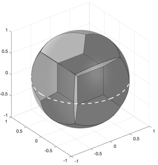
(b) Sphere domain

Figure 1: Computational domains

Non-conforming test.

We focus on the case in which the knot vectors of one patch are a refinement of the knot vectors of the adjacent one: this allows the use of the properties of the knot insertion algorithm to glue the degrees-of-freedom of the interface and properly modify the gluing matrix $\mathbf{B}$ (see [31, Section 5.2]).

Let $\Omega=(0,1)\times(0,3)\times(0,1)$ be a domain on which we consider a Dirichlet boundary value problem. We choose the problem data so that the exact solution is $\boldsymbol{u}(x,y,z)=[\cos{x},\ z\sin{y},\ (xyz)^{2}]^{T}$. The domain is divided into three patches, with increasing levels of refinement (see Figure 1a). In particular, we set $n_{el}^{(1)}=2^{2}$ in the leftmost patch, $n_{el}^{(2)}=2^{3}$ in the central patch, and $n_{el}^{(3)}=2^{4}$ in the rightmost one.

Table 1: Preconditioners comparison - non-conforming test on the parallelepiped domain

EXACT INEXACT ${p}$ Iter. Time (s) Iter. Time (s) 1 53 00119 086 02 2 57 00283 096 03 3 63 1 080 104 06 4 67 3 740 111 12

In Table 1 we report the results for the EXACT and INEXACT approaches. The INEXACT local solvers yield to a number of iterations that is less than twice the number of iterations of the EXACT choice. On the contrary, the solving times of the INEXACT local solvers are orders of magnitudes less than the times of the EXACT local solvers. In all cases, the number of iterations is only mildly dependent on $p$.

Sphere domain test.

Let $\Omega$ be the unitary sphere with center in the origin that is divided into 7 patches: an inner cube and six patches around it (see Figure 1b). We remark that the sphere patches are described by NURBS parametrizations and that the isogeometric local spaces used for the discretization are spaces of mapped NURBS. However, the INEXACT local solvers are still built using B-splines and some information on the weights of the NURBS basis functions, as well as some information about the geometry maps, is incorporated into the solvers as described in Section 5.2.3. We choose the problem data so that the exact solution is $\boldsymbol{u}(x,y,z)=[\cos{x},\ z\sin{y},\ (xyz)^{2}]^{T}$. We impose Dirichlet boundary conditions on $\partial\Omega\cap\{z\leq 0\}$, while Neumann conditions are imposed on the rest of the boundary, i.e. on $\partial\Omega\cap\{z>0\}$. Note that in classical IETI setting, this choice of b.c. provides local problems without a tensor product structure.

In this test we consider an equal number of element in each parametric direction of each patch, i.e. we set $n_{el}^{(1)}=\dots=n_{el}^{(7)}=:n_{el}$. We report the numerical results in Table 2 for an increasing number of $n_{el}$ and for NURBS of degree 4 and 5. The INEXACT approach is orders of magnitude faster that the EXACT one, even though the number of iterations is higher.

Table 2: Preconditioners comparison - sphere domain test.

$p=4$ $p=5$ EXACT INEXACT EXACT INEXACT ${n_{el}}$ Iter. Time (s) Iter. Time (s) Iter. Time (s) Iter. Time (s) 02 61 000007 123 005 065 0000022 146 007 04 73 000056 146 009 079 0000160 172 016 08 87 02 757 184 026 100 005 764 225 056 16 97 63 699 217 132 105 275 500 246 277

Weak scalability test.

In this test we consider the weak scalability of the AF-IETI preconditioned method: we keep the dimension of each subproblem fixed and we increase the number of patches. In particular, we consider a cube domain $\Omega=(0,1)^{3}$. We choose the problem data so that the exact solution is $\boldsymbol{u}(x,y,z)=[\cos{x},\ z\sin{y},\ (xyz)^{2}]^{T}$. We consider Neumann boundary conditions on $\partial\Omega\cap\{x=0\}$ and $\partial\Omega\cap\{x=1\}$ and Dirichlet boundary conditions on the remaining faces. We split the domain $\Omega$ into an increasing number $\mathcal{N}_{patch}$ of equal cubes, keeping $p=3$ and $n_{el}^{(1)}=\dots=n_{el}^{(\mathcal{N}_{patch})}=2^{3}$.

Table 3: Preconditioners comparison - weak scalability test.

EXACT INEXACT $\mathcal{N}_{patch}$ Iter. Time (s) Iter. Time (s) ${2^{3}}$ 48 00007 090 02 ${3^{3}}$ 52 00057 097 07 ${4^{3}}$ 53 00275 100 18 ${5^{3}}$ 56 1 030 105 36 ${6^{3}}$ 57 3 019 105 63

Table 3 shows that the number of iterations of both the EXACT and INEXACT solvers is independent of the number pf patches, that is, the solvers are scalable. Again, the INEXACT variant saves orders of magnitudes of computational time. In the scalability test the computational time reflects the single-core sequential solving of local problems. Clearly, a parallel implementation would lead to a decrease of the computational time for both solvers.

7 Conclusions

In this paper, we studied a combination of the FD solver with a domain decomposition method of FETI type in a general multi-patch isogeometric setting, where the subdomains of the method coincide with the isogeometric patches. We focused on the All-Floating (domain) version of FETI, where both the continuity and Dirichlet boundary conditions are weakly imposed by Lagrange multipliers. We built a preconditioner for the resulting saddle-point linear system in which the FD method is used in the inexact solvers for the local problems. We also proved the spectral estimates that guarantee the good convergence properties of the preconditioned iterative solver. The comparison of the performances of the exact and inexact local solvers in the preconditioner on three dimensional compressible linear elasticity model problems clearly showed that the inexact choice brings great improvements, in terms of computational time. Numerical results demonstrated the weak scalability is not affected by introducing the inexact solvers, and that the overall approach is quite robust with respect to the spline degree $p$. The variant of the inexact local solvers that includes also some information on the geometry parametrization performs well also with distorted geometries.

We remark that while the present work is focused on IgA, the range of applicability of AF-IETI with FD-based inexact solvers is in fact not limited to IgA problems. Indeed, the presented approach is suitable for any discretization where the domain is split into a number of non-overlapping subdomains, on each of which the discretization has a tensor structure, like e.g. the spectral element method.

References

- [1] L. Beirão da Veiga, A. Buffa, J. Rivas, and G. Sangalli. Some estimates for ––-refinement in Isogeometric Analysis. Numerische Mathematik, 118(2):271–305, 2011.
- [2] L. Beirão da Veiga, D. Cho, L. F. Pavarino, and S. Scacchi. Overlapping Schwarz methods for isogeometric analysis. SIAM J. Numer. Anal., 50(3):1394–1416, 2012.
- [3] L. Beirão da Veiga, D. Cho, L. F. Pavarino, and S. Scacchi. BDDC preconditioners for isogeometric analysis. Math. Models Methods Appl. Sci., 23(06):1099–1142, 2013.
- [4] M. Bercovier and I. Soloveichik. Overlapping non matching meshes domain decomposition method in isogeometric analysis. arXiv preprint arXiv:1502.03756, 2015.
- [5] A. Bressan and E. Sande. Approximation in FEM, DG and IGA: a theoretical comparison. Numerische Mathematik, 143(4):923–942, 2019.
- [6] N. Collier, L. Dalcin, D. Pardo, and V. M. Calo. The cost of continuity: performance of iterative solvers on isogeometric finite elements. SIAM J. Sci. Comput., 35(2):A767–A784, 2013.
- [7] N. Collier, D. Pardo, L. Dalcin, M. Paszynski, and V. M. Calo. The cost of continuity: a study of the performance of isogeometric finite elements using direct solvers. Comput. Methods Appl. Mech. Engrg., 213/216:353–361, 2012.
- [8] J. A. Cottrell, T. J. R. Hughes, and Y. Bazilevs. Isogeometric analysis: toward integration of CAD and FEA. John Wiley & Sons, 2009.
- [9] C. de Boor. A practical guide to splines, volume 27 of Applied Mathematical Sciences. Springer-Verlag, New York, revised edition, 2001.
- [10] F. de Prenter, C.V. Verhoosel, and E.H. van Brummelen. Preconditioning immersed isogeometric finite element methods with application to flow problems. Comp. Methods Appl. Mech. Engrg., 348:604 – 631, 2019.
- [11] S. Diliberto and E. Straus. On the approximation of a function of several variables by the sum of functions of fewer variables. Pacific J. Math., 1(2):195–210, 1951.
- [12] Z. Dostál, D. Horák, and R. Kučera. Total FETI-an easier implementable variant of the FETI method for numerical solution of elliptic PDE. Comm. Numer. Methods Engrg., 22(12):1155–1162, 2006.
- [13] John A Evans, Yuri Bazilevs, Ivo Babuška, and Thomas JR Hughes. -Widths, sup–infs, and optimality ratios for the -version of the isogeometric finite element method. Comput. Methods Appl. Mech. Engrg., 198(21-26):1726–1741, 2009.
- [14] C. Farhat, J. Mandel, and F. X. Roux. Optimal convergence properties of the FETI domain decomposition method. Comp. Methods Appl. Mech. Engrg., 115(3-4):365–385, 1994.
- [15] C. Farhat and F. X. Roux. A method of finite element tearing and interconnecting and its parallel solution algorithm. Internat. J. Numer. Methods Engrg., 32(6):1205–1227, 1991.
- [16] G. H. Golub and C. F. Van Loan. Matrix computations. JHU Press, 2012.
- [17] C. Hofer and U. Langer. Dual-primal isogeometric tearing and interconnecting solvers for multipatch dG-IgA equations. Comput. Methods Appl. Mech. Engrg., 316:2–21, 2017.
- [18] C. Hofer, U. Langer, and S. Takacs. Inexact dual-primal isogeometric tearing and interconnecting methods. In International Conference on Domain Decomposition Methods, pages 393–403. Springer, 2017.
- [19] T. J. R. Hughes, J. A. Cottrell, and Y. Bazilevs. Isogeometric analysis: CAD, finite elements, NURBS, exact geometry and mesh refinement. Comput. Methods Appl. Mech. Engrg., 194(39-41):4135–4195, 2005.
- [20] A. Klawonn and O. B. Widlund. A domain decomposition method with Lagrange multipliers and inexact solvers for linear elasticity. SIAM J. Sci. Comput., 22(4):1199–1219, 2000.
- [21] S. K. Kleiss, C. Pechstein, B. Jüttler, and S. Tomar. IETI–isogeometric tearing and interconnecting. Comput. Methods Appl. Mech. Engrg., 247:201–215, 2012.
- [22] R. E. Lynch, J. R. Rice, and D. H. Thomas. Direct solution of partial difference equations by tensor product methods. Numerische Mathematik, 6(1):185–199, 1964.
- [23] J. Mandel and R. Tezaur. Convergence of a substructuring method with Lagrange multipliers. Numerische Mathematik, 73(4):473–487, 1996.
- [24] A. Mantzaflaris, B. Jüttler, B. N. Khoromskij, and U. Langer. Low rank tensor methods in Galerkin-based isogeometric analysis. Comput. Methods Appl. Mech. Engrg., 316:1062–1085, 2017.
- [25] M. Montardini, M. Negri, G. Sangalli, and M. Tani. Space-Time Least-Squares Isogeometric Method for Parabolic Problems. arXiv preprint arXiv:1809.10026, 2018.
- [26] M. Montardini, G. Sangalli, and M. Tani. Robust isogeometric preconditioners for the Stokes system based on the Fast Diagonalization method. Comput. Methods Appl. Mech. Engrg., 2018.
- [27] G. Of and O. Steinbach. The all-floating boundary element tearing and interconnecting method. Journal of numerical mathematics, 17(4):277–298, 2009.
- [28] L. F. Pavarino and S. Scacchi. Isogeometric block FETI-DP preconditioners for the Stokes and mixed linear elasticity systems. Comput. Methods Appl. Mech. and Engrg., 310:694–710, 2016.
- [29] C. Pechstein. Finite and Boundary Element Tearing and Interconnecting Methods for Multiscale Elliptic Partial Differential Equations. PhD thesis, JKU, 2008.
- [30] C. Pechstein. Finite and boundary element tearing and interconnecting solvers for multiscale problems, volume 90. Springer Science & Business Media, 2012.
- [31] L. Piegl and W. Tiller. The NURBS book. Springer Science & Business Media, 2012.
- [32] E. Sande, C. Manni, and H. Speleers. Sharp error estimates for spline approximation: Explicit constants, n-widths, and eigenfunction convergence. Math. Models Methods Appl. Sci., pages 1–31, 2019.
- [33] G. Sangalli and M. Tani. Isogeometric preconditioners based on fast solvers for the Sylvester equation. SIAM J. Sci. Comput., 38(6):A3644–A3671, 2016.
- [34] G. Sangalli and M. Tani. Matrix-free weighted quadrature for a computationally efficient isogeometric -method. Comput. Methods Appl. Mech. Engrg., 338:117–133, 2018.
- [35] S. Takacs. Robust approximation error estimates and multigrid solvers for isogeometric multi-patch discretizations. Math. Models Methods Appl. Sci., 28(10):1899–1928, 2018.
- [36] S. Takacs and T. Takacs. Approximation error estimates and inverse inequalities for B-splines of maximum smoothness. Math. Models Methods Appl. Sci., 26(07):1411–1445, 2016.
- [37] A. Toselli and O. Widlund. Domain decomposition methods—algorithms and theory, volume 34 of Springer Series in Computational Mathematics. Springer-Verlag, Berlin, 2005.
- [38] R. Vázquez. A new design for the implementation of isogeometric analysis in Octave and Matlab: GeoPDEs 3.0. Comput. Math. Appl., 72(3):523–554, 2016.
- [39] E. L. Wachspress. Generalized ADI preconditioning. Comput. Math. Appl., 10(6):457–461, 1984.