Shapley value confidence intervals for
attributing variance explained

Abstract

The coefficient of determination, the $R^{2}$, is often used to measure the variance explained by an affine combination of multiple explanatory covariates. An attribution of this explanatory contribution to each of the individual covariates is often sought in order to draw inference regarding the importance of each covariate with respect to the response phenomenon. A recent method for ascertaining such an attribution is via the game theoretic Shapley value decomposition of the coefficient of determination. Such a decomposition has the desirable efficiency, monotonicity, and equal treatment properties. Under a weak assumption that the joint distribution is pseudo-elliptical, we obtain the asymptotic normality of the Shapley values. We then utilize this result in order to construct confidence intervals and hypothesis tests regarding such quantities. Monte Carlo studies regarding our results are provided. We found that our asymptotic confidence intervals are computationally superior to competing bootstrap methods and are able to improve upon the performance of such intervals. In an expository application to Australian real estate price modelling, we employ Shapley value confidence intervals to identify significant differences between the explanatory contributions of covariates, between models, which otherwise share approximately the same $R^{2}$ value. These different models are based on real estate data from the same periods in 2019 and 2020, the latter covering the early stages of the arrival of the novel coronavirus, COVID-19.

1 Introduction

The multiple linear regression model (MLR) is among the most commonly applied tools for statistics inference; see [Seber and Lee, 2003] and [Greene, 2007, Part I] for thorough introductions to MLR models. In the usual MLR setting, one observes an independent and identically distributed (IID) sample of data pairs $\bm{Z}_{i}^{\top}=\left(Y_{i},\bm{X}_{i}^{\top}\right)\in\mathbb{R}^{d+1}$, where $i\in\left[n\right]=\left\{1,\dots,n\right\}$, and $d,n\in\mathbb{N}$. The MLR model is then defined via the linear relationship

$$\mathbb{E}\left(Y_{i}|\bm{X}_{i}=\bm{x}_{i}\right)=\beta_{0}+\sum_{i=1}^{d}\beta_{j}X_{ij}\text{,}$$

where $\bm{\beta}^{\top}=\left(\beta_{0},\dots,\beta_{n}\right)\in\mathbb{R}^{d+1}$, and $\bm{X}_{i}^{\top}=\left(X_{i1},\dots,X_{id}\right)$. We shall also write $\bm{Z}_{i}^{\top}=\left(Z_{i0},Z_{i1},\dots,Z_{id}\right)$, when it is convenient to do so. Here, $\left(\cdot\right)^{\top}$ is the transposition operator.

The usual nomenclature is to call the $Y_{i}$ and $\bm{X}_{i}$ elements of each pair, the response (or dependent) variable and the explanatory (or covariate) vector, respectively. Here, the $j$th element of $\bm{X}_{i}$: $X_{ij}$ ($j\in\left[d\right]$), is referred to as the $j\text{th}$ explanatory variable (or the $j\text{th}$ covariate). We may put the pairs of data into a dataset $\mathcal{Z}_{n}=\left\{\bm{Z}_{i}\right\}_{i=1}^{n}$.

Let $R_{jk}\left(\mathcal{Z}_{n}\right)$ denote the sample correlation coefficient

$$R_{jk}\left(\mathcal{Z}_{n}\right)=\frac{\sum_{i=1}^{n}\left(Z_{ij}-\bar{Z}_{j}\right)\left(Z_{ik}-\bar{Z}_{k}\right)}{\sqrt{\sum_{i=1}^{n}\left(Z_{ij}-\bar{Z}_{j}\right)^{2}}\sqrt{\sum_{i=1}^{n}\left(Z_{ik}-\bar{Z}_{k}\right)^{2}}}\text{,}$$ (1)

for each $j,k\in\left\{0\right\}\cup\left[d\right]$. Here $\bar{Z}_{j}=n^{-1}\sum_{i=1}^{n}Z_{ij}$ is the sample mean of variable $j$. Write $\mathcal{U}\subseteq\left\{0\right\}\cup\left[d\right]$ be a nonempty subset, where $\mathcal{U}=\left\{u_{1},\dots,u_{\left|\mathcal{U}\right|}\right\}$, where $\left|\mathcal{U}\right|$ is the cardinality of $\mathcal{U}$. We refer to the matrix of correlations between the variables in $\mathcal{U}$ as

$$\mathbf{C}_{n}\left(\mathcal{U}\right)=\left[\begin{array}[]{cccc}1&R_{u_{1}u_{2}}\!\left(\mathcal{Z}_{n}\right)&\cdots&R_{u_{1}u_{\left|U\right|}}\!\left(\mathcal{Z}_{n}\right)\\ R_{u_{2}u_{1}}\!\left(\mathcal{Z}_{n}\right)&\phantom{\Big{|}}1&\cdots&R_{u_{2}u_{\left|\mathcal{U}\right|}}\!\left(\mathcal{Z}_{n}\right)\\ \vdots&\vdots&\ddots&\vdots\\ R_{u_{\left|\mathcal{U}\right|}u_{1}}\!\left(\mathcal{Z}_{n}\right)&R_{u_{\left|\mathcal{U}\right|}u_{2}}\!\left(\mathcal{Z}_{n}\right)&\cdots&1\end{array}\right]\text{.}$$ (2)

A common inferential task is to determine the degree to which the response can be explained by the covariate vector, in totality. The usual device for addressing this question is via the coefficient of determination (or squared coefficient of multiple correlation), which is defined as

$$R^{2}\left(\mathcal{Z}_{n}\right)=1-\frac{\left|\mathbf{C}_{n}\left(\left\{0\right\}\cup\left[d\right]\right)\right|}{\left|\mathbf{C}_{n}\left(\left[d\right]\right)\right|}\text{,}$$ (3)

where $\left|\mathbf{C}\right|$ is the matrix determinant of $\mathbf{C}$ (cf. [Cowden, 1952]). Intuitively, the coefficient of determination measures the proportion of the total variation in the response variable that is explained by variation in the covariate vector. See [Seber and Lee, 2003, Sec. 4.4] and [Greene, 2007, Sec. 3.5] for details regarding the derivation and interpretation of the $R^{2}\left(\mathcal{Z}_{n}\right)$ coefficients.

A refinement to the question that is addressed by the $R^{2}\left(\mathcal{Z}_{n}\right)$ coefficient, is that of eliciting the contribution of each of the covariates to the total value of $R^{2}\left(\mathcal{Z}_{n}\right)$.

In the past, this question has partially been resolved via the use of partial correlation coefficients (see, e.g. [Greene, 2007, Sec. 3.4]). Unfortunately, such coefficients are only able to measure the contribution of each covariate coefficient of determination, conditional to the presence of other covariates that are already in the MLR model.

A satisfactory resolution to the question above, is provided by [Lipovetsky and Conklin, 2001], [Israeli, 2007], and [Huettner and Sunder, 2012], who each suggested and argued for the use of the Shapley decomposition of [Shapley, 1953]. The Shapley decomposition is a game-theoretic method for decomposing the contribution to the value of a utility function in the context of cooperative games.

Let $\bm{\pi}^{\top}=\left(\pi_{1},\dots,\pi_{d}\right)$ be a permutation of the set $\left[d\right]$. For each $j\in\left[d\right]$, let

$$\mathcal{S}_{j}\left(\bm{\pi}\right)=\left\{k\,:\,\pi_{k}<\pi_{j},\,k\in\left[d\right]\right\}$$

be the elements of $[d]$ that appear before $\pi_{j}$ when $[d]$ is permuted by $\bm{\pi$}.Wemaydefine$R_S_j(π)^2(Z_n)$and$R_{ j} ∪S_j(π)^2(Z_n)$inasimilarmannerto\eqref{eq: R2 definition},usingthegenericdefinition\begin{equation}R_{\mathcal{S}}^{2}\left(\mathcal{Z}_{n}\right)=1-\frac{\left|\mathbf{C}_{n}\left(\left\{0\right\}\cup\mathcal{S}\right)\right|}{\left|\mathbf{C}_{n}\left(\mathcal{S}\right)\right|}\text{,}\end{equation}fornonemptysubsets$S⊆[d]$,and$R_{ }^2(Z_n)=0$fortheemptyset.\par Treatingthecoefficientofdeterminationasautilityfunction,wemayconductaShapleypartitionofthe$R^2(Z_n)$coefficientbycomputingthe$jth$Shapleyvalue,foreachofthe$d$covariates,definedby\begin{equation}V_{j}\left(\mathcal{Z}_{n}\right)=\left|\mathcal{P}\right|^{-1}\sum_{\bm{\pi}\in\mathcal{P}}\left[R_{\left\{j\right\}\cup\mathcal{S}_{j}\left(\bm{\pi}\right)}^{2}\left(\mathcal{Z}_{n}\right)-R_{\mathcal{S}_{j}\left(\bm{\pi}\right)}^{2}\left(\mathcal{Z}_{n}\right)\right]\text{,}\end{equation}where$P$isthesetofallpossiblepermutationsof$[d]$.\par Comparedtootherdecompositionsofthecoefficientofdetermination,suchasthoseconsideredin\cite[cite]{[\@@bibref{}{Gromping:2006aa}{}{}]}and\cite[cite]{[\@@bibref{}{Gromping:2007aa}{}{}]},theShapleyvalues,obtainedfromthepartitioningabove,havethefavorableaxiomaticpropertiesthatwerewellexposedin\cite[cite]{[\@@bibref{}{Huettner:2012aa}{}{}]}.Specifically,theShapleyvalueshavetheefficiency,monotonicity,and,equaltreatmentproperties,andthedecompositionisprovablytheonlymethodthatsatisfiesallthreeoftheseproperties(cf.\cite[cite]{[\@@bibref{}{Young:1985aa}{}{}, Thm. 2]}).Here,inthecontextofthecoefficientofdetermination,efficiency,monotonicity,andequaltreatmentaredefinedasfollows:\par\begin{description}\par\par\description@item@[Efficiency:] The sum of the Shapley values across all covariates equates to the coefficient of determination, that is $$\sum_{j=1}^{d}V_{j}\left(\mathcal{Z}_{n}\right)=R^{2}\left(\mathcal{Z}_{n}\right).$$ \par\par\description@item@[Monotonicity:] For pairs of samples $\mathcal{Z}_{m}$ and $\mathcal{Z}_{n}$, of sizes $m,n\in\mathbb{N}$, $$R_{\left\{j\right\}\cup\mathcal{S}_{j}\left(\bm{\pi}\right)}^{2}\left(\mathcal{Z}_{n}\right)-R_{\mathcal{S}_{j}\left(\bm{\pi}\right)}^{2}\left(\mathcal{Z}_{n}\right)\geq R_{\left\{j\right\}\cup\mathcal{S}_{j}\left(\bm{\pi}\right)}^{2}\left(\mathcal{Z}_{m}\right)-R_{\mathcal{S}_{j}\left(\bm{\pi}\right)}^{2}\left(\mathcal{Z}_{m}\right)\text{,}$$ for every $\bm{\pi}\in\mathcal{P}$, implies that $V_{j}\left(\mathcal{Z}_{n}\right)\geq V_{j}\left(\mathcal{Z}_{m}\right)$, for each $j\in[d]$. \par\par\description@item@[Equal treatment:] If covariates $j,k\in\left[d\right]$ are substitutes in the sense that $$R_{\left\{j\right\}\cup\mathcal{S}_{j}\left(\bm{\pi}\right)}^{2}\left(\mathcal{Z}_{n}\right)=R_{\left\{k\right\}\cup\mathcal{S}_{k}\left(\bm{\pi}\right)}^{2}\left(\mathcal{Z}_{n}\right)\text{,}$$ for each $\bm{\pi}\in\mathcal{P}$ such that $k\notin\mathcal{S}_{j}\left(\bm{\pi}\right)$ and $j\notin\mathcal{S}_{k}\left(\bm{\pi}\right)$, then the Shapley decomposition is such that $V_{j}\left(\mathcal{Z}_{n}\right)=V_{k}\left(\mathcal{Z}_{n}\right)$. \par\par\end{description}\par Wenotethatequaltreatmentisalsooftenreferredtoassymmetryintheliterature.TheuniquenessoftheShapleydecompositioninexhibitingthethreedescribedpropertiesisoftenusedasthejustificationforitsapplication.Furthermore,therearenumeroussetsofaxiomaticpropertiesthatleadtotheShapleyvaluedecompositionasasolution(see,e.g.,\cite[cite]{[\@@bibref{}{feltkamp1995alternative}{}{}]}).Inthestatisticsliterature,itisknownthattheaxiomsfordecompositionofthecoefficientofdeterminationthatareproposedby\cite[cite]{[\@@bibref{}{kruskal1987relative}{}{}]}correspondexactlytotheShapleyvalues(cf.\cite[cite]{[\@@bibref{}{genizi1993decomposition}{}{}]}).\par Whenconductingstatisticalestimationandcomputation,theassumptionofrandomnessofdatanecessitatesthatweaddressnotonlytheproblemofpointestimation,butalsovariabilityquantification.In\cite[cite]{[\@@bibref{}{Huettner:2012aa}{}{}]},variabilityforthecoefficientofdeterminationShapleyvalueswerequantifiedviatheuseofbootstrapconfidenceintervals(CIs).Combinedwiththeusualcomputationalintensivenessofbootstrapresampling(see,e.g.,\cite[cite]{[\@@bibref{}{Efron:1988aa}{}{}]}and\cite[cite]{[\@@bibref{}{Baglivo:2005aa}{}{}, Ch. 12]}),thecombinatorynatureofthecomputationof\eqref{eq: shapley value}(noticethat$|P|=d!$)compoundsthetimecomplexityofsuchamethod,whichisalreadyoforder$O(2^d)$.Inthisarticle,weseektoprovideanasymptoticmethodforcomputingCIsfortheShapleyvalues.\par Ourapproachusesthejointasymptoticnormalityresultoftheelementsinacorrelationmatrix,underanellipticalassumption,via\cite[cite]{[\@@bibref{}{Steiger:1984aa}{}{}]},combinedwithasymptoticnormalityresultsconcerningthedeterminantsofacorrelationmatrix,of\cite[cite]{[\@@bibref{}{Hedges:1983ab}{}{}]}and\cite[cite]{[\@@bibref{}{Olkin:1995aa}{}{}]}.Usingtheseresults,wederivetheasymptoticjointdistributionforthe$R^2(Z_n)$Shapleyvalues,whichallowsustoconstructCIsforeachofthevaluesandtheircontrasts.WeassessthefinitesamplepropertiesofourconstructionsviaacomprehensiveMonteCarlostudyanddemonstratetheuseofourCIsviaapplicationstorealestatepricedata.\par Theremainderofthearticleproceedsasfollows.InSection\ref{sec:main},wepresentourmainresultsregardingtheasymptoticdistributionofthecoefficientofdeterminationShapleyvalues,andtheirCIconstructions.InSection\ref{s: monte},wepresentacomprehensiveMonteCarlostudyofourCIconstructionmethod.InSection\ref{sec:realestate},wedemonstratehowourresultscanbeappliedtorealestatepricedata.ConclusionsarelastlydrawninSection\ref{sec:discussion}.$

2 Main results

2.1 The correlation matrix

Let $\bm{Z}\in\mathbb{R}^{d+1}$ be a random variable with mean vector $\bm{\mu}\in\mathbb{R}^{d+1}$ and covariance matrix $\bm{\Sigma}\in\mathbb{R}^{\left(d+1\right)\times\left(d+1\right)}$. Then, we can define the coefficient of multivariate kurtosis [Mardia, 1970] by

$$\kappa=\frac{1}{\left(d+1\right)\left(d+3\right)}\mathbb{E}\left[\left(\bm{Z}-\bm{\mu}\right)^{\top}\bm{\Sigma}^{-1}\left(\bm{Z}-\bm{\mu}\right)\right]^{2}\text{.}$$

Let $\rho_{jk}=\text{cor}\left(Z_{j},Z_{k}\right)$, for $j,k\in\left\{0\right\}\cup\left[d\right]$ such that $j\neq k$. Assume that $\bm{Z}$ arises from an elliptical distribution (cf. [Fang et al., 1990, Ch. 2]) and let $\mathcal{Z}_{n}$ be an IID sample with the same distribution as $\bm{Z}$. Then, we may estimate $\rho_{jk}$ using the sample correlation coefficient (1). Upon writing acov to denote the asymptotic covariance, we have the following result due to Corollary 1 of [Steiger and Browne, 1984].

Lemma 1.

If $\bm{Z}$ arises from an elliptical distribution and has coefficient of multivariate kurtosis $\kappa$, then the normalized coefficients of correlation $\zeta_{jk}=n^{1/2}\left(R_{jk}-\rho_{jk}\right)$ ($j,k\in\left\{0\right\}\cup\left[d\right]$; $j\neq k$) converge to a jointly normal distribution with asymptotic mean and covariance elements $0$ and

$$\text{acov}\!\left(\zeta_{gh},\zeta_{jk}\right) = \kappa\left[\rho_{gh}\rho_{jk}\left(\rho_{gj}^{2}+\rho_{hj}^{2}+\rho_{gk}^{2}+\rho_{hk}^{2}\right)/2+\rho_{gj}\rho_{hk}+\rho_{gk}\rho_{hj}\right]$$ (6)

$$-\kappa\left[\rho_{gh}\left(\rho_{hj}\rho_{hk}+\rho_{gj}\rho_{gk}\right)+\rho_{jk}\left(\rho_{gj}\rho_{hj}+\rho_{gk}\rho_{hk}\right)\right]\text{.}$$

Remark 1.

We note that the elliptical distribution assumption above can be replaced by a broader pseudo-elliptical assumption, as per [Yuan and Bentler, 1999] and [Yuan and Bentler, 2000]. This is a wide class of distributions that includes some that may not be symmetric. Due to the complicated construction of the class, we refer the interested reader to the source material for its definition.

Remark 2.

We may state a similar result that replaces the elliptical assumption by a fourth moments existence assumption instead, using Proposition 2 of [Steiger and Browne, 1984]. In order to make practical use of such an assumption, we require the estimation of $\left(d+1\right)!$/$\left[\left(d-3\right)!4!\right]$ fourth order moments instead of a single kurtosis term $\kappa$. Such a result may be useful when the number of fourth order moments is small, but become infeasible rapidly, as $d$ increases.

Let $\mathcal{V}\subseteq\left\{0\right\}\cup\left[d\right]$, where $\mathcal{V}=\left\{v_{1},\dots,v_{\left|\mathcal{V}\right|}\right\}$. Define $\mathbf{C}_{n}\left(\mathcal{V}\right)$ in the same manner as (2), and let

$$\mathbf{R}\left(\mathcal{U}\right)=\left[\begin{array}[]{cccc}1&\rho_{u_{1}u_{2}}&\cdots&\rho_{u_{1}u_{\left|\mathcal{U}\right|}}\\ \rho_{u_{2}u_{1}}&1&\cdots&\rho_{u_{2}u_{\left|\mathcal{U}\right|}}\\ \vdots&\vdots&\ddots&\vdots\\ \rho_{u_{\left|\mathcal{U}\right|}u_{1}}&\rho_{u_{\left|\mathcal{U}\right|}u_{2}}&\cdots&1\end{array}\right]$$

and

$$\mathbf{R}\left(\mathcal{V}\right)=\left[\begin{array}[]{cccc}1&\rho_{v_{1}v_{2}}&\cdots&\rho_{v_{1}v_{\left|\mathcal{V}\right|}}\\ \rho_{v_{2}v_{1}}&1&\cdots&\rho_{v_{2}v_{\left|\mathcal{V}\right|}}\\ \vdots&\vdots&\ddots&\vdots\\ \rho_{v_{\left|\mathcal{V}\right|}v_{1}}&\rho_{v_{\left|\mathcal{V}\right|}v_{2}}&\cdots&1\end{array}\right]\text{.}$$

The following theorem is adapted from a result of [Hedges and Olkin, 1983b] (also appearing as Theorem 1 in [Hedges and Olkin, 1983a]). Our result expands upon the original theorem, to allow for inference regarding elliptically distributed data, and not just normally distributed data. We further fix some typographical matters that appear in both [Hedges and Olkin, 1983a] and [Hedges and Olkin, 1983b].

Lemma 2.

Assume the same conditions as in (1). Then, the normalized covariance determinant $\delta\!\left(\mathcal{U}\right)=n^{1/2}\left(\left|\mathbf{C}_{n}\left(\mathcal{U}\right)\right|-\left|\mathbf{R}\left(\mathcal{U}\right)\right|\right)$ (where $\mathcal{U}$ and $\mathcal{V}$ are nonempty subsets of $\left\{0\right\}\mathcal{\cup}\left[d\right]$) converges to a jointly normal distribution, with asymptotic mean and covariance elements $0$ and

$$\text{acov}\!\left(\delta\!\left(\mathcal{U}\right),\delta\!\left(\mathcal{V}\right)\right)=\sum_{g,h\in\mathcal{U}}\sum_{j,k\in\mathcal{V}}r_{\mathcal{U}}\left(g,h\right)r_{\mathcal{V}}\left(j,k\right)\text{acov}\!\left(\zeta_{gh},\zeta_{jk}\right)\text{,}$$ (7)

where $\text{acov}\!\left(\zeta_{gh},\zeta_{jk}\right)$ is as per (6),

$$\begin{bmatrix}r_{\mathcal{U}}\!\left(\,u_{1},u_{1}\right)&r_{\mathcal{U}}\!\left(\,u_{1},u_{2}\right)&\cdots&r_{\mathcal{U}}\!\left(\,u_{1},u_{\left|\mathcal{U}\right|}\right)\\ r_{\mathcal{U}}\!\left(\,u_{2},u_{1}\right)&r_{\mathcal{U}}\!\left(\,u_{2},u_{2}\right)&\cdots&r_{\mathcal{U}}\!\left(\,u_{2},u_{\left|\mathcal{U}\right|}\right)\\ \vdots&\vdots&\ddots&\vdots\\ r_{\mathcal{U}}\!\left(u_{\left|\mathcal{U}\right|},u_{1}\right)&r_{\mathcal{U}}\!\left(u_{\left|\mathcal{U}\right|},u_{2}\right)&\cdots&r_{\mathcal{U}}\!\left(u_{\left|\mathcal{U}\right|},u_{\left|\mathcal{U}\right|}\right)\end{bmatrix}=\left|\mathbf{R}\left(\mathcal{U}\right)\right|\mathbf{R}^{-1}\left(\mathcal{U}\right)\text{,}$$

and $r_{\mathcal{V}}\left(j,k\right)$ ($j,k\in\mathcal{V}$) is defined similarly.

Proof.

The result is due to an application of the delta method (see, e.g., [van der Vaart, 1998, Thm. 3.1]) and the fact that for any matrix $\mathbf{R}$, the derivative of its determinant is $\partial\left|\mathbf{R}\right|/\partial\mathbf{R}=\left|\mathbf{R}\right|\mathbf{R}^{-\top}$ [Seber, 2008, Sec. 17.45]. Notice that we use the unconstrained case of the determinant derivative, since we sum over each pair of coordinates, where $g\neq h$ or $j\neq k$, twice. ∎

Remark 3.

If $\mathbf{R}$ is symmetric, then $\partial\left|\mathbf{R}\right|/\partial\mathbf{R}=\left|\mathbf{R}\right|\left[2\mathbf{R}^{-1}-\text{diag}\left(\mathbf{R}^{-1}\right)\right]$ [Seber, 2008, Sec. 17.45]. Using this fact, we may write (7) in the alternative, and more computationally efficient form

$$\text{acov}\!\left(\delta\!\left(\mathcal{U}\right),\delta\!\left(\mathcal{V}\right)\right)=\sum_{\begin{subarray}{c}g\leq h\\ g,h\in\mathcal{U}\end{subarray}}\sum_{\begin{subarray}{c}j\leq k\\ j,k\in\mathcal{V}\end{subarray}}r_{\mathcal{U}}^{*}\left(g,h\right)r_{\mathcal{V}}^{*}\left(j,k\right)\text{acov}\!\left(\zeta_{gh},\zeta_{jk}\right)\text{,}$$

where

$$\begin{bmatrix}r_{\mathcal{U}}^{*}\!\left(\,u_{1},u_{1}\right)&r_{\mathcal{U}}^{*}\!\left(\,u_{1},u_{2}\right)&\cdots&r_{\mathcal{U}}^{*}\!\left(\,u_{1},u_{\left|\mathcal{U}\right|}\right)\\ r_{\mathcal{U}}^{*}\!\left(\,u_{2},u_{1}\right)&r_{\mathcal{U}}^{*}\!\left(\,u_{2},u_{2}\right)&\cdots&r_{\mathcal{U}}^{*}\!\left(\,u_{2},u_{\left|\mathcal{U}\right|}\right)\\ \vdots&\vdots&\ddots&\vdots\\ r_{\mathcal{U}}^{*}\!\left(u_{\left|\mathcal{U}\right|},u_{1}\right)&r_{\mathcal{U}}^{*}\!\left(u_{\left|\mathcal{U}\right|},u_{2}\right)&\cdots&r_{\mathcal{U}}^{*}\!\left(u_{\left|\mathcal{U}\right|},u_{\left|\mathcal{U}\right|}\right)\end{bmatrix} = 2\left|\mathbf{R}\left(\mathcal{U}\right)\right|\mathbf{R}^{-1}\left(\mathcal{U}\right)$$

$$- \left|\mathbf{R}\left(\mathcal{U}\right)\right|\text{diag}\left(\mathbf{R}^{-1}\left(\mathcal{U}\right)\right)\text{,}$$

and $r_{\mathcal{V}}^{*}\left(j,k\right)$ ($j,k\in\mathcal{V}$) is defined similarly.

2.2 The coefficient of determination

Let plim denote convergence in probability, so that for any sequence $\{X_{n}\}$, and any random variable $X$, the statement

$$\lim_{n\rightarrow\infty}\Pr(|X_{n}-X|>\varepsilon)=0\,,$$

for every $\varepsilon>0$, can be written as $\operatorname*{plim}_{n\rightarrow\infty}X_{n}=X$.

Now, recall definition (4), and further let $\rho_{\mathcal{S}}^{2}=\operatorname*{plim}_{n\rightarrow\infty}R_{\mathcal{S}}^{2}\left(\mathcal{Z}_{n}\right)$. We adapt from and expand upon [Hedges and Olkin, 1983a, Thm. 2] in the following result. This result also fixes typographical errors that appear in the original theorem, as well as in [Hedges and Olkin, 1983b].

Lemma 3.

Assume the same conditions as in 1. Then, the normalize coefficient of determination $\lambda\left(\mathcal{S}\right)=n^{1/2}\left(R_{\mathcal{S}}^{2}\left(\mathcal{Z}_{n}\right)-\rho_{\mathcal{S}}^{2}\right)$ (where $S$ and $\mathcal{T}$ are nonempty subsets of $\left[d\right]$) converges to a jointly normal distribution, with asymptotic mean and covariance elements $0$ and

$$\text{acov}\!\left(\lambda\!\left(\mathcal{S}\right),\lambda\!\left(\mathcal{T}\right)\right) = \frac{1}{\left|\mathbf{R}\left(\mathcal{S}\right)\right|\left|\mathbf{R}\left(\mathcal{T}\right)\right|}\text{ acov}\!\left(\delta\!\left(\left\{0\right\}\cup\mathcal{S}\right),\delta\!\left(\left\{0\right\}\cup\mathcal{T}\right)\right)$$ (8)

$$+\frac{\left|\mathbf{R}\left(\left\{0\right\}\cup\mathcal{S}\right)\right|\left|\mathbf{R}\left(\left\{0\right\}\cup\mathcal{T}\right)\right|}{\left|\mathbf{R}\left(\mathcal{S}\right)\right|^{2}\left|\mathbf{R}\left(\mathcal{T}\right)\right|^{2}}\text{acov}\!\left(\delta\!\left(\mathcal{S}\right),\delta\!\left(\mathcal{T}\right)\right)$$

$$-\frac{\left|\mathbf{R}\left(\left\{0\right\}\cup\mathcal{S}\right)\right|}{\left|\mathbf{R}\left(\mathcal{S}\right)\right|^{2}\left|\mathbf{R}\left(\mathcal{T}\right)\right|}\text{acov}\!\left(\delta\!\left(\mathcal{S}\right),\delta\!\left(\left\{0\right\}\cup\mathcal{T}\right)\right)$$

$$-\frac{\left|\mathbf{R}\left(\left\{0\right\}\cup\mathcal{T}\right)\right|}{\left|\mathbf{R}\left(\mathcal{S}\right)\right|\left|\mathbf{R}\left(\mathcal{T}\right)\right|^{2}}\text{acov}\!\left(\delta\!\left(\left\{0\right\}\cup\mathcal{S}\right),\delta\!\left(\mathcal{T}\right)\right)\text{.}$$

Proof.

We apply the delta method again, using the functional form (4), and using the fact that

$$\frac{\partial}{\partial\left(x,y\right)}\left(1-\frac{x}{y}\right)=\left(-\frac{1}{y},\frac{x}{y^{2}}\right)\text{.}$$

∎

Remark 4.

When $\mathcal{S}=\mathcal{T}$, (8) yields the usual form for the asymptotic variance of $R_{\mathcal{S}}^{2}\left(\mathcal{Z}_{n}\right)$: $4\kappa\rho_{\mathcal{S}}^{2}\left(1-\rho_{\mathcal{S}}^{2}\right)^{2}$ (cf. [Yuan and Bentler, 2000]).

2.3 The Shapley values

For every $j\in\left[d\right]$ and $\mathcal{S}\subseteq\mathcal{S}_{j}=\left[d\right]-\left\{j\right\}$, there are $\left|\mathcal{S}\right|!\left(d-\left|\mathcal{S}\right|-1\right)!$ elements of $\bm{\pi}\in\mathcal{P}$ such that $\mathcal{S}_{j}\left(\bm{\pi}\right)=\mathcal{S}$. Thus, we may write

$$V_{j}\left(\mathcal{Z}_{n}\right)=\sum_{\mathcal{S}\subseteq\mathcal{S}_{j}}\omega\left(\mathcal{S}\right)\left[R_{\left\{j\right\}\cup\mathcal{S}}^{2}\left(\mathcal{Z}_{n}\right)-R_{\mathcal{S}}^{2}\left(\mathcal{Z}_{n}\right)\right]\text{,}$$ (9)

where $\omega\left(\mathcal{S}\right)=\left|\mathcal{S}\right|!\left(d-\left|\mathcal{S}\right|-1\right)!/d!$, and define $v_{j}=\operatorname*{plim}_{n\rightarrow\infty}V_{j}\left(\mathcal{Z}_{n}\right)$. Using this functional form (9), we may apply the delta method once more, in order to derive the following joint asymptotic normal distribution result regarding the Shapley values $V_{j}\left(\mathcal{Z}_{n}\right)$, for $j\in\left[d\right]$.

Remark 5.

The form (9) is a useful computational trick that reduces the computational time of form (5) and results in more efficient computations for fixed $d$. It is unclear whether other formulations such as that of [Hart et al., 1988] can make the computation time even faster. Unfortunately, however, there is no formulation that reduces the $\mathcal{O}(2^{d})$ scaling, as $d$ increases.

Theorem 1.

Assume the same conditions as in 1. Then, the normalized Shaply values $\xi_{j}=n^{1/2}\left(V_{j}\left(\mathcal{Z}_{n}\right)-v_{j}\right)$ (where $j,k\in\left[d\right]$) converge to a jointly normal distribution, with asymptotic mean and covariance elements $0$ and $\text{acov}\!\left(\xi_{j},\xi_{k}\right)=a_{jk}+b_{jk}-c_{jk}-d_{jk}$. Here,

$$a_{jk}=\sum_{\mathcal{S}\subseteq\mathcal{S}_{j}}\sum_{\mathcal{T}\subseteq\mathcal{S}_{k}}\omega\left(\mathcal{S}\right)\omega\left(\mathcal{T}\right)\text{acov}\!\left(\lambda\left(\left\{j\right\}\cup\mathcal{S}\right),\lambda\left(\left\{k\right\}\cup\mathcal{T}\right)\right)\text{,}$$

$$b_{jk}=\sum_{\mathcal{S}\subseteq\mathcal{S}_{j}}\sum_{\mathcal{T}\subseteq\mathcal{S}_{k}}\omega\left(\mathcal{S}\right)\omega\left(\mathcal{T}\right)\text{acov}\!\left(\lambda\left(\mathcal{S}\right),\lambda\left(\mathcal{T}\right)\right)\text{,}$$

$$c_{jk}=\sum_{\mathcal{S}\subseteq\mathcal{S}_{j}}\sum_{\mathcal{T}\subseteq\mathcal{S}_{k}}\omega\left(\mathcal{S}\right)\omega\left(\mathcal{T}\right)\text{acov}\!\left(\lambda\left(\mathcal{S}\right),\lambda\left(\left\{k\right\}\cup\mathcal{T}\right)\right)\text{,}$$

and

$$d_{jk}=\sum_{\mathcal{S}\subseteq\mathcal{S}_{j}}\sum_{\mathcal{T}\subseteq\mathcal{S}_{k}}\omega\left(\mathcal{S}\right)\omega\left(\mathcal{T}\right)\text{acov}\!\left(\lambda\left(\left\{j\right\}\cup\mathcal{S}\right),\lambda\left(\mathcal{T}\right)\right)\text{,}$$

where $\lambda\left(\mathcal{S}\right)$ is as defined in 3, for nonempty subsets $\mathcal{S}\subseteq\left[d\right]$.

Using the result above, we may apply the delta method again in order to construct asymptotic CIs or hypothesis tests regarding any continuous function of the $d$ Shapley values for the coefficient of determination. Of particular interest is the asymptotic CI for each of the individual Shapley values and the hypothesis test for the difference between two Shapley values.

The asymptotic $100\left(1-\alpha\right)\%$ CI for the $j\text{th}$ expected Shapley value $v_{j}$ has the usual form

$$\left(V_{j}\left(\mathcal{Z}_{n}\right)-\Phi^{-1}\left(1-\frac{\alpha}{2}\right)\sqrt{\frac{\text{avar}\left(\xi_{j}\right)}{n}},V_{j}\left(\mathcal{Z}_{n}\right)+\Phi^{-1}\left(1-\frac{\alpha}{2}\right)\sqrt{\frac{\text{avar}\left(\xi_{j}\right)}{n}}\right)\text{,}$$

where $\text{avar}\left(\xi_{j}\right)=\text{acov}\!\left(\xi_{j},\xi_{j}\right)$ denotes the asymptotic variance of $\xi_{j}$ and $\Phi^{-1}$ is the inverse cumulative distribution function of the standard normal distribution. The $z$-statistic for the test of the null and alternative hypotheses

$$\text{H}_{0}:v_{j}=v_{k}\text{ and }\text{H}_{1}:v_{j}\neq v_{k}\text{,}$$ (10)

for $j,k\in\left[d\right]$ such that $j\neq k$, is

$$\Delta_{n}=\frac{\sqrt{n}\left(V_{j}\left(\mathcal{Z}_{n}\right)-V_{k}\left(\mathcal{Z}_{n}\right)\right)}{\sqrt{\text{avar}\left(\xi_{j}\right)+\text{avar}\left(\xi_{k}\right)-2\text{acov}\!\left(\xi_{j},\xi_{k}\right)}}\text{,}$$

where $\Delta_{n}$ has an asymptotic standard normal distribution.

Remark 6.

In practice, we do not know the necessary elements $\kappa$ and $\rho_{jk}$ $\left(j,k\in\left\{0\right\}\cup\left[d\right];j\neq k\right)$ that are required in order to specify the asymptotic covariance terms in 1–3 and 1. However, by Slutsky’s theorem, we have the usual result that any acov (or avar) term can be replaced by the estimator $\widehat{\text{acov}}_{n}$ (or $\widehat{\text{avar}}_{n}$), which replaces $\kappa$ by the estimator of [Mardia, 1970]

$$\hat{\kappa}\left(\mathcal{Z}_{n}\right)=\frac{\sum_{i=1}^{n}\left[\left(\bm{Z}_{i}-\bar{\bm{Z}}\right)^{\top}\hat{\bm{\Sigma}}_{n}^{-1}\left(\left\{0\right\}\cup\left[d\right]\right)\left(\bm{Z}_{i}-\bar{\bm{Z}}\right)\right]^{2}}{n\left(d+1\right)\left(d+3\right)}\text{,}$$

and replaces $\rho_{jk}$ by $R_{jk}\left(\mathcal{Z}_{n}\right)$, where $\bar{\bm{Z}}^{\top}=\left(\bar{Z}_{0},\dots,\bar{Z}_{d}\right)$. Here,

$$\hat{\bm{\Sigma}}_{n}\left(\mathcal{\mathcal{U}}\right)=\left[\begin{array}[]{cccc}\hat{\Sigma}_{u_{1}u_{1}}\left(\mathcal{Z}_{n}\right)&\hat{\Sigma}_{u_{1}u_{2}}\left(\mathcal{Z}_{n}\right)&\cdots&\hat{\Sigma}_{u_{1}u_{\left|\mathcal{U}\right|}}\left(\mathcal{Z}_{n}\right)\\ \hat{\Sigma}_{u_{2}u_{1}}\left(\mathcal{Z}_{n}\right)&\hat{\Sigma}_{u_{2}u_{2}}\left(\mathcal{Z}_{n}\right)&\cdots&\hat{\Sigma}_{u_{2}u_{\left|\mathcal{U}\right|}}\left(\mathcal{Z}_{n}\right)\\ \vdots&\vdots&\ddots&\vdots\\ \hat{\Sigma}_{u_{\left|\mathcal{U}\right|}u_{1}}\left(\mathcal{Z}_{n}\right)&\hat{\Sigma}_{u_{\left|\mathcal{U}\right|}u_{2}}\left(\mathcal{Z}_{n}\right)&\cdots&\hat{\Sigma}_{u_{\left|\mathcal{U}\right|}u_{\left|\mathcal{U}\right|}}\left(\mathcal{Z}_{n}\right)\end{array}\right],$$

where $\hat{\Sigma}_{jk}\left(\mathcal{Z}_{n}\right)$ is the sample covariance between the $j$th and $k$th dimension of $\bm{Z}$ ($j,k\in\{0\}\cup[d]$). For example, the estimated test statistic

$$\hat{\Delta}_{n}=\frac{\sqrt{n}\left(V_{j}\left(\mathcal{Z}_{n}\right)-V_{k}\left(\mathcal{Z}_{n}\right)\right)}{\sqrt{\widehat{\text{avar}}_{n}\left(\xi_{j}\right)+\widehat{\text{avar}}_{n}\left(\xi_{k}\right)-2\widehat{\text{acov}}_{n}\left(\xi_{j},\xi_{k}\right)}}\text{,}$$ (11)

for the hypotheses (10), retains the property of having an asymptotically standard normal distribution.

3 Monte Carlo studies and benchmarks

In each of the following three Monte Carlo studies, we simulate a large number $N$ of random samples $\mathcal{Z}_{n}^{(i)},\;i\in[N]$, of size $n$, from a chosen distribution $\mathcal{D}$. For each sample, we apply 1 to calculate an asymptotic 95% CI for the first Shapley value $v_{1}$, producing a set of $N$ observed intervals $\mathcal{I}_{N}=\left\{[\ell_{i},u_{i}]\,:\,i\in[N]\right\}$, as realisations of the CI $[L,U]$ for $v_{1}$. The coverage probability $\text{covr}_{v_{1}}([L,U]):=\Pr(v_{1}\in[L,U])$ is then estimated as the proportion of intervals in $\mathcal{I}_{N}$ containing the population Shapley value

$$\widehat{\text{covr}}_{v_{1}}([L,U])=\frac{|\{[\ell_{i},u_{i}]\in\mathcal{I}_{N}\,:\,v_{1}\in[\ell_{i},u_{i}]\}|}{N}.$$ (12)

Here, the population Shapley value $v_{1}$ has the form:

$$v_{1}=\sum_{\mathcal{S}\subseteq\mathcal{S}_{1}}\omega\left(\mathcal{S}\right)\left[R_{\left\{1\right\}\cup\mathcal{S}}^{2}-R_{\mathcal{S}}^{2}\right],$$

where $R_{\mathcal{S}}^{2}$ is defined by replacing $\mathbf{C}_{n}$ in (4) by the known population correlation matrix $\text{cor}(\mathbf{Z}),$ as determined by the chosen distribution $\mathcal{D}$. In Studies A and B, this population correlation matrix is the $(d+1)\times(d+1)$ matrix $\mathbf{\Sigma}$, with diagonal elements equal to 1 and off-diagonal elements equal to a constant correlation $c\in[0,1)$. That is,

$$\mathbf{\Sigma}=c\,\mathbf{J}_{d+1}+(1-c)\,\mathbf{I}_{d+1},$$ (13)

where $\mathbf{J}_{d+1}$ denotes a $(d+1)\times(d+1)$ matrix with all entries equal to $1$. Note that, for fixed variance, larger magnitudes of $c$ map to larger regression coefficients. Thus, these simulations can be viewed as assigning equal regression coefficients to each covariates that are increasing for increasing values of $c$.

In Study C, we are concerned with covariance matrices with off-diagonal elements deviating from $c$. We aim to capture a case where the off-diagonal elements of $\text{cor}(\mathbf{Z})$ are not uniform, and where some may be negative. This is achieved by sampling $\mathcal{Z}_{n}^{(i)}$ from a multivariate normal distribution $\mathcal{D}_{i}$, with a symmetric positive definite covariance matrix $\mathbf{\Sigma}_{i}$ that is sampled at random from a Wishart distribution with scale matrix $\mathbf{\Sigma}$; see Section 3.3. Accordingly, the population Shapley value $v_{1}^{(i)}$ is unique to sample $i$, and thus we adjust the coverage estimator $\widehat{\text{covr}}_{v_{1}}([L,U])$ by replacing $v_{1}$ on the RHS of 12 by $v_{1}^{(i)}$.

To accompany our estimates of $\widehat{\text{covr}}_{v_{1}}([L,U])$, we also provide Clopper-Pearson CIs [Clopper and Pearson, 1934] for the coverage probability. We also report the average CI widths, and middle 95% percentile intervals for the widths. For comparison, we estimate coverage probabilities of non-parametric bootstrap confidence intervals in each of the three studies. To obtain the bootstrap CIs, we set some large number $N_{b}$ and take random resamples $\mathcal{R}_{n}^{(r)},r\in[N_{b}]$, of size $n$, with replacement, from $\mathcal{Z}^{(i)}_{n}$. From these resamples, we calculate the set of estimated Shapley values $\mathcal{L}_{i}=\left\{V_{1}\left(\mathcal{R}_{n}^{(r)}\right)\,:\,r\in[N_{b}]\right\}$. The $i$th 95% bootstrap CI is then taken as the middle 95% percentile interval of $\mathcal{L}$, and the coverage is estimated as in 12.

To obtain results for each pair $(n,c)\in\mathcal{N}\times\mathcal{C}$, where $\mathcal{N}=\{5,10,\ldots,50\}\cup\{100,200,\ldots,2000\}$ and $\mathcal{C}=\{0,0.1,0.2,0.3,0.6,0.9,0.99\}$, we performed $30\times 7=210$ simulations for each of the three studies. We use $N=N_{b}=1000$ and $d=3$, in all cases.

3.1 MC Study A

Here, we choose $\mathcal{D}=N_{d+1}(\mathbf{0},\mathbf{\Sigma})$, so that each sample $\mathcal{Z}^{(i)}_{n},$ for $i\in[N],$ is drawn from a multivariate normal distribution, with covariance $\mathbf{\Sigma}$ given in (13).

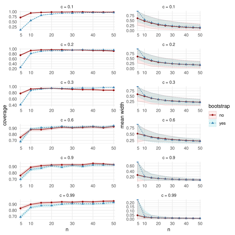
Figure 12: Comparisons of coverage (left column) and mean width (right column), between the bootstrap CIs (dashed lines with triangular markers) and the asymptotic CIs (solid lines with circular markers) in MC Study A. Rows represent correlations $c$, increasing from $0.1$ on the top row to $0.99$ on the bottom row. The horizontal axes display the sample sizes $n=5,10,\ldots,50$.

The simulation results in Figure 1 (and in Figure 12, Appendix A) show very similar coverage and width performance between the two assessed CIs for moderate and high correlations $c>0.3$. For lower correlations $c\leq 0.2$, coverage convergence appears to be slower in $n$ than the bootstrap CI for large sample sizes ($n\geq 100$). The opposite trend seems to hold for small sample sizes ($n\leq 50$), see the discussion under MC Study C. Also, for the highest correlation $c=0.99$, coverage performance of the asymptotic CI is overall slightly better than the bootstrap CI.

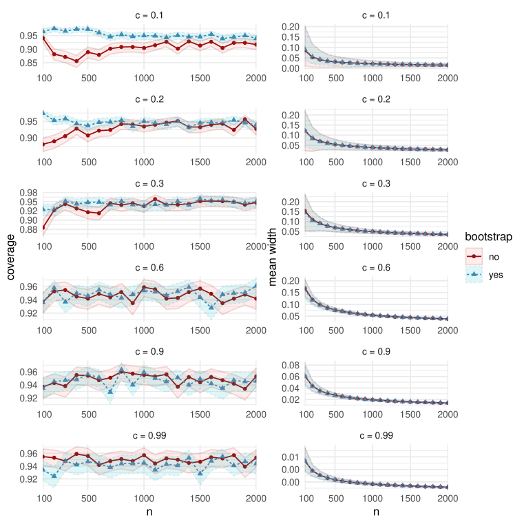
Figure 1: Comparisons of coverage (left column) and mean width (right column), between the bootstrap CIs (dashed lines with triangular markers) and the asymptotic CIs (solid lines with circular markers) in MC Study A. Rows represent correlations $c$, increasing from $0.1$ on the top row to $0.99$ on the bottom row. The horizontal axes display the sample sizes $n=100,200,\ldots,2000$.

3.2 MC Study B

Here, we choose $\mathcal{D}=t_{\nu}(\mathbf{0},\mathbf{\Sigma})$ where $t_{\nu}(\mathbf{\mu},\mathbf{\Sigma})$ is the multivariate Student $t$ distribution with $\nu\in(0,\infty)$ degrees of freedom, mean vector $\mathbf{\mu},$ and scale matrix $\mathbf{\Sigma}.$ Specifically, the $i$th sample $\mathcal{Z}^{(i)}_{n}$, for $i\in[N]$, we set $\nu=100$ degrees of freedom, and set $\mathbf{\Sigma}$ as the $(d+1)\times(d+1)$ covariance matrix in 13.

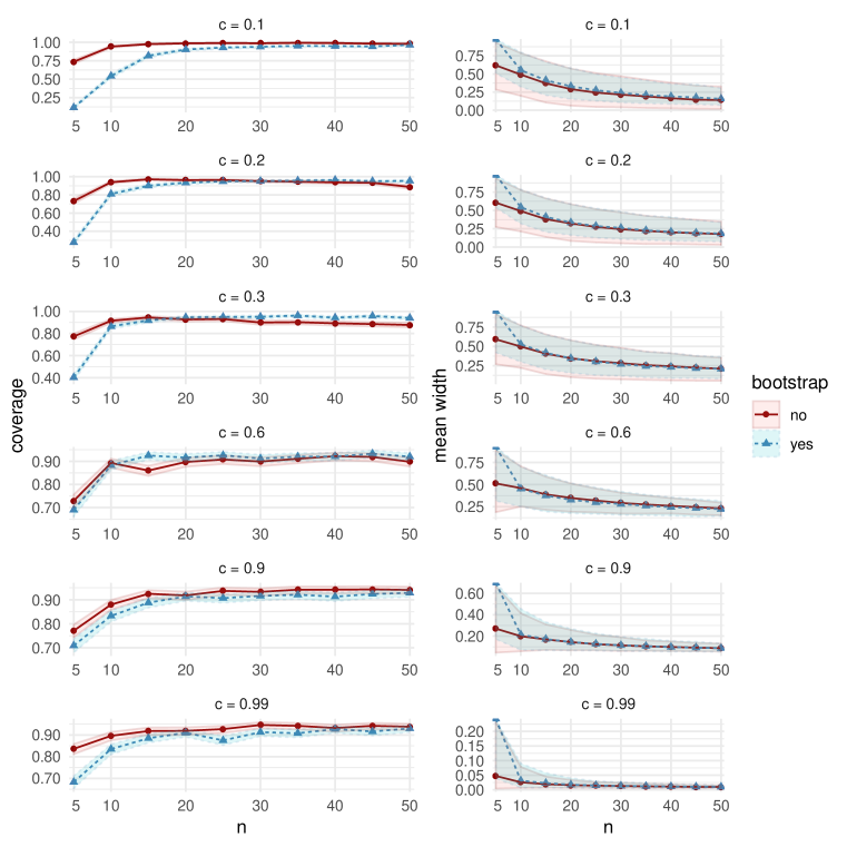
Figure 13: Comparisons of coverage (left column) and mean width (right column), between the bootstrap CIs (dashed lines with triangular markers) and the asymptotic CIs (solid lines with circular markers) in MC Study B. Rows represent correlations $c$, increasing from $0.1$ on the top row to $0.99$ on the bottom row. The horizontal axes display the sample sizes $n=5,10,\ldots,50$.

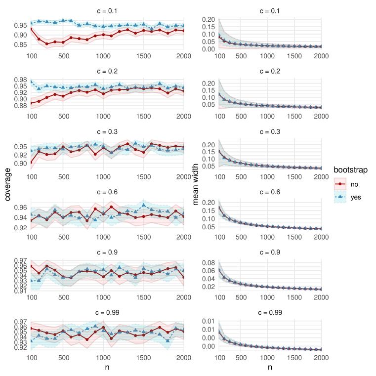
Figure 14: Comparisons of coverage (left column) and mean width (right column), between the bootstrap CIs (dashed lines with triangular markers) and the asymptotic CIs (solid lines with circular markers) in MC Study B. Rows represent correlations $c$, increasing from $0.1$ on the top row to $0.99$ on the bottom row. The horizontal axes display the sample sizes $n=100,200,\ldots,2000$.

For all sample sizes $n$ and correlations $c$, coverage and width performances are similar to MC Study A (see Figure 13 and Figure 14 in Appendix A). Of particular interest, in both MC Studies A and B (but not in MC Study C), we observe that for $c=0$, the estimated coverage probability of the asymptotic CI is almost equal to 1, for all sample sizes greater than 10, while the corresponding bootstrap CIs have estimated coverage equal to 0 (Figure 2 left). Despite this, the average CI widths, though large under small samples, are somewhat smaller than those for bootstrap (Figure 2 right).

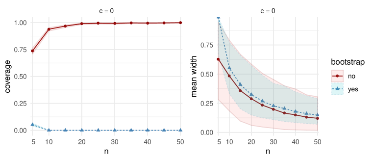
Figure 2: Comparisons of coverage (left column) and mean width (right column) between bootstrap CIs (dashed lines with triangular markers) and the asymptotic CIs (solid lines with circular markers) in MC Study B, for correlation $c=0$. The horizontal axes display the sample sizes $n=5,10,\ldots,50$.

3.3 MC Study C

Here, we set $\mathcal{D}_{i}=N_{d+1}(0,\mathbf{\Sigma}_{i})$, so that the sample $\mathcal{Z}^{(i)}_{n}$, for $i\in N$, is drawn from a multivariate normal distribution, with covariance matrix $\mathbf{\Sigma}_{i}$ realised from a Wishart distribution $W_{d+1}(\mathbf{\Sigma},\nu)$ with scale matrix $\mathbf{\Sigma}$ and $\nu$ degrees of freedom. This set up is different from Studies A and B in that the distributions $\mathcal{D}_{i}$, and therefore the population Shapley values $v_{1}^{(i)}$, are allowed to differ between samples.

The distribution $W_{d+1}(\mathbf{\Sigma},\nu)$ can be understood as the distribution of the sample covariance matrix of a sample of size $\nu+1$ from the distribution $N_{d+1}(0,\mathbf{\Sigma})$ (cf [Fujikoshi et al., 2011]). This implies that each covariance matrix $\mathbf{\Sigma}_{i}$ can have non-uniform and negative off-diagonal elements, with variability between the off-diagonal elements increasing as $\nu$ decreases. For this study, we set $\nu=100$.

Aside for the case $c=0$, coverage and width statistics are again similar to MC Studies A and B, for all $n$ and $c$ (see Appendix A). Interestingly, in all three Studies, for small sample sizes ($n\leq 50$), coverage is often higher than for the bootstrap CI, with slightly smaller average widths, as seen in Figure 3 (and in Figure 12 and Figure 13 in Appendix A). For the $c=0$ case, the observed behaviour differs from MC Studies A and B, with bootstrap performing comparatively well for large sample sizes (Figure 4).

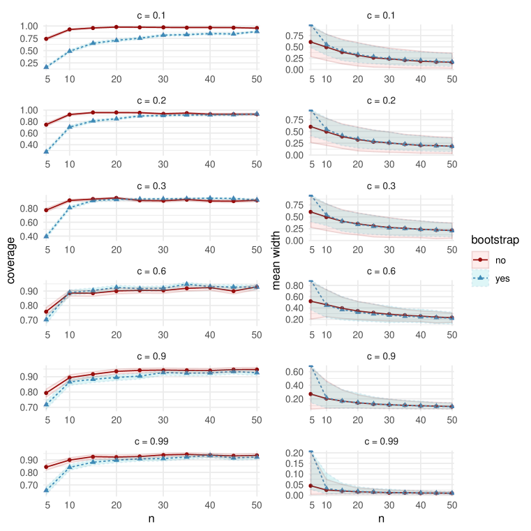
Figure 3: Comparisons of coverage (left column) and mean width (right column), between the bootstrap CIs (dashed lines with triangular markers) and the asymptotic CIs (solid lines with circular markers) in MC Study C. Rows represent correlations $c$, increasing from $0.1$ on the top row to $0.99$ on the bottom row. The horizontal axes display the sample sizes $n=5,10,\ldots,50$.

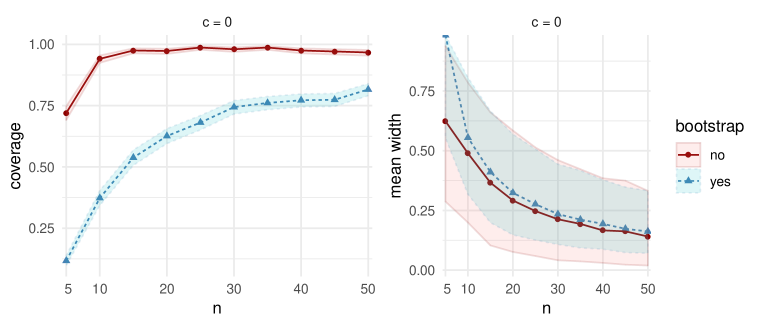
Figure 4: Comparisons of coverage (left column) and mean width (right column) between bootstrap CIs (dashed lines with triangular markers) and the asymptotic CIs (solid lines with circular markers) in MC Study C, for correlation $c=0$. The horizontal axes display the sample sizes $n=5,10,\ldots,50$.

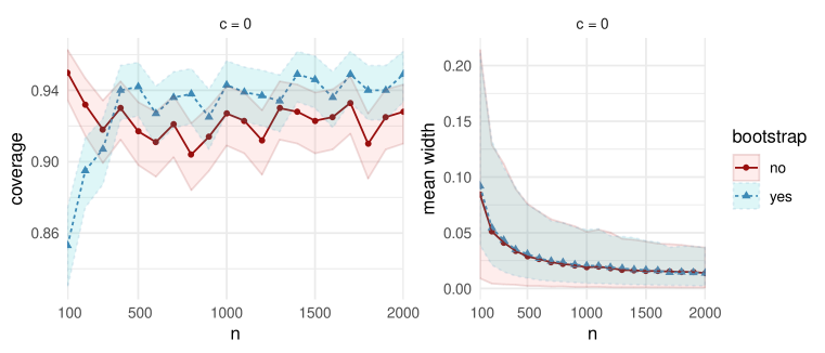
Figure 5: Comparisons of coverage (left column) and mean width (right column) between bootstrap CIs (dashed lines with triangular markers) and the asymptotic CIs (solid lines with circular markers) in MC Study C, for correlation $c=0$. The horizontal axes display the sample sizes $n=100,200,\ldots,2000$.

3.4 Computational benchmarks

From Figure 6, we see that the memory usage (left) and mean execution time (right) for the bootstrap CIs are both higher than that for the asymptotic CIs, and that the ratio increases with sample size. As $n$ increases, asymptotic CIs become increasingly efficient, compared to the bootstrap CIs. On the other hand, as $d$ increases, with $n$ fixed, we expect an increase in the relative efficiency of the bootstrap, since the complexity of calculating $\text{acov}(\xi_{j},\xi_{k})$ in 1 grows faster in $d$ than the complexity of the bootstrap procedure.

Table 1: Parameters for computational benchmarking.

Parameter	Value(s)
Number of features ($d$)	3
Sample sizes ($n$)	1000, 5000, 10000
Number of bootstrap resamples ($N_{b}$)	1000
Number of simulation repetitions ($N$)	1000

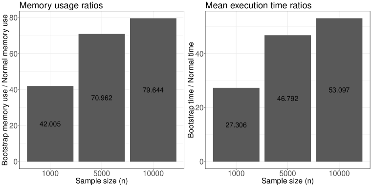
Figure 6: Computational benchmark metric ratios of confidence interval estimation using the naïve bootstrap over the asymptotic normality approach.

3.5 Summary of results and recommendations for use

Below follows a summary of the general tendencies and observations from our results, and recommendations regarding when to use the asymptotic CIs.

• For all correlations $c$ in all three Studies, the estimated coverage probability of asymptotic intervals is above $0.85$ for all sample sizes $n\geq 10$.

• For smaller correlations and sample sizes, in particular $c\geq 0.2$ and $n>15$, the lower bound of the confidence interval for coverage never drops below $0.85$.

• For all correlations $c\geq 0.3$ and sample sizes $n>100$, the lower bound of the confidence interval for coverage never drops below $0.9$.

• For small correlations, in particular $c\leq 0.1$ and sample sizes $10\leq n\leq 100$, the lower bound of the confidence interval for the coverage of the asymptotic CIs never drops below $0.91$.

• For $c=0$ and $n\geq 15$, the lower bound of the asymptotic CI for coverage never drops below $0.95$ in Studies A and B, while in Study C the lower bound is at least $0.88$.

• For sample sizes $15\leq n\leq 50$, the coverage of the asymptotic CI tends to be higher when $c$ is closer to the boundaries of $[0,1]$, as shown in Figure 7.

• The average asymptotic CI width is lower when $c$ is nearer to the boundaries of $[0,1]$, see Figure 8.

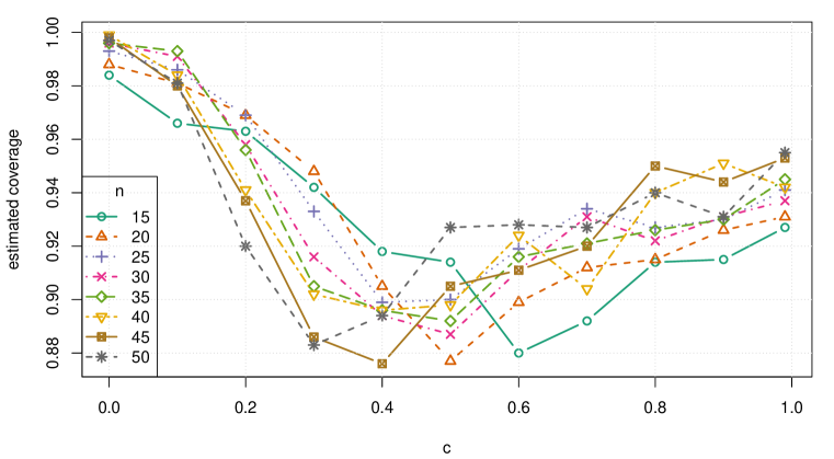
Figure 7: Estimated coverage probability versus correlation $c$, for small samples sizes $n=15,20,\ldots,50$, in MC Study A. The same patterns can be observed for Studies B and C.

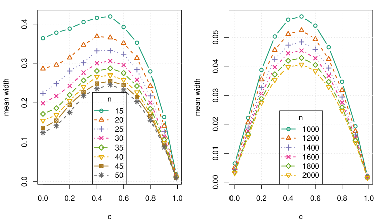
Figure 8: Average confidence interval width versus correlation $c$, for small sample sizes $n=15,20,\ldots,50$ (left) and large sample sizes $n=1000,1200,\ldots,2000$ (right), in MC Study A. The same patterns are present in MC Study B and C.

We now make some general observations which apply to all three Studies. As sample size increases, the estimated coverage initially increases rapidly, as can be seen, for example, in the left column of Figure 3. For small sample sizes between $n=5$ and $n=50$, the asymptotic CIs typically outperform bootstrap CIs, especially when $c$ lies farther from $0.5$; there is a clear drop in coverage as $c$ approaches $0.5$, for small samples, as can be seen in Figure 7. In many cases, the estimated coverage is above $0.9$ for $n\geq 10$. However, empirical coverage does not appear to be an increasing function of sample size in general. On the top row in the left column of Figure 1, we observe one example of a clear and extended dip in coverage for $n$ in $[100,1000]$. This gives rise to the general observation that the asymptotic intervals have preferable coverage statistics over bootstrap for small samples, but not for a certain range of large samples, depending on $c$.

We further observe that, for all $n$, there is a general increase in the average CI width as $c$ approaches $0.5$ from either direction, as in Figure 8. In all Studies, over all sample sizes and correlations, the bootstrap CI average widths were smaller than the asymptotic CI widths by at most $0.0289$, and vice versa by at most $0.0667$. In general, the asymptotic intervals display favourable widths, though less so near $c=0.5$.

Based on these observations, we recommend using asymptotic CIs over bootstrap CIs under the following conditions:

1. Computational time is relevant (e.g., estimating a large number of Shapley values).

2. The sample size is small (e.g., $n\leq 50$).

3. The correlation between explanatory variables and the response variable is expected to be beyond $\pm 0.2$ from $0.5$, or when this is where the highest precision is desired.

We note that our observations are made from an incomplete albeit comprehensive set of simulation scenarios. There are of course an infinite number of combinations of simulation cases and thus we cannot guarantee that our observation applies to all possible DGPs.

4 Application: Melbourne real estate and COVID-19

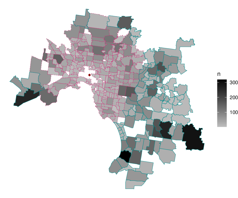
Figure 11: Map of Melbourne suburbs included in this study, with greyscale shading to represent sample sizes. Pink dashed polygon borders contain suburbs classified as near to the Central Business District (i.e., $\leq 25$km), and blue solid polygon borders represent those classified as far ($>25$km). The solid red diamond represents the location of the CBD.

For an interesting application of our methods, in this section we identify significant changes in the behaviour of the local real estate market in Melbourne, Australia, within the period from 1 February to 1 April, between the years 2019 and 2020. In 2020, this corresponds to an early period of growing public concern regarding the novel coronavirus COVID-19. We obtain the Shapley decomposition of the coefficient of multiple correlation $R^{2}$ between observed house prices and a number of property features. We also find significant differences in behaviour between real estate near and far from the Central Business District (CBD), where near is defined to be within $25\,\mathrm{km}$ of Melbourne CBD, and far is defined as non-near (see Figure 11). Note that the nature of this investigation is exploratory and expository; our conclusions are not intended to be taken as evidence for the purposes of policy or decision making.

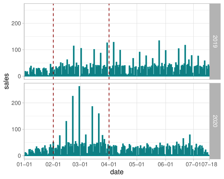
Figure 10: Bar plot of sales per day between 1 January and 18 July in 2019 and 2020. Vertical dashed red lines indicate 1 February and 1 April, between which a spike in sales is observed.

On 1 February the Australian government announced a temporary ban on foreign arrivals from mainland China, and by 1 April a number of social distancing measures were in place. We scraped real estate data from the AUHousePrices website (https://www.auhouseprices.com/), to obtain a data set of $13{,}291$ (clean) house sales between 1 January and 18 July in 2019 and 2020. We then reduced this date range to capture only the spike in sales observed between 1 February and 1 April (see Figure 10), giving a remaining sample size of $5110$, which was partitioned into the four subgroups in Table 2. Within each of the four subgroups we perform a Yeo-Johnson transformation [Yeo and Johnson, 2000] to reduce any violation of the assumption of joint pseudo-ellipticity.

Table 2: The four subgroups and their sample sizes after partitioning by distance (where near $:=$ within $25\,\mathrm{km}$ of CBD), and year of sale in the period 1 February to 1 April 2019 and 2020.

Subgroup:	near (2019)	far (2019)	near (2020)	far (2020)
Sample size:	1203	953	1824	1130

We decompose $R^{2}$ amongst the covariates: distance to CBD (CBD); images used in advertisement (images); property land size (land); distance to nearest school (school); distance to nearest station (station); and number of bedrooms $+$ bathrooms $+$ car ports (room); along with the response variable, house sale price (price). We expect the room covariate to act as a proxy for house size. Thus we decompose $R^{2}$ for the linear model,

$$\mathbb{E}(\text{price})=\beta_{0}+\bm{\beta}(\text{CBD},\,\text{images},\,\text{land},\,\text{school},\,\text{station},\,\text{room})^{T},\;\;\beta_{0}\in\mathbb{R},\,\bm{\beta}\in\mathbb{R}^{6}.$$ (14)

Fitted to each of the four subgroups, we obtain $R^{2}=0.37$ for model (14), for each subgroup except for the near (2020) subgroup, for which $R^{2}=0.39$. The resulting Shapley values and 95% confidence intervals are listed in Table 3, and shown graphically in Figure 9. From those results we make the following observations regarding attributions of the total variability in house prices explained by model (14):

1. In both 2019 and 2020, the attribution for distance to CBD was significantly higher for house sales near to the CBD, compared to house sales farther from the CBD. Correspondingly, the attribution for roominess was significantly lower for house sales near to the CBD.

2. Amongst sales that were near to the CBD, distances to the CBD received significantly greater attribution than both land size and roominess in 2019. Unlike the case for sales that were far from the CBD, these differences remained significant in 2020.

3. Distances to stations and schools, as well as images used in advertising, have apparently had little overall impact. In all four subgroups, the attribution for distance to the nearest school is not significantly different from $0$. However, distance to a station does receive significantly more attribution amongst houses that are near to the CBD, compared to those farther away.

4. Interestingly, while not a significant result, the number of images used in advertising did appear to receive greater attribution amongst house sales that were far from the CBD, compared to those near to it.

5. Amongst sales that were far from the CBD, land size and roominess both received significantly more attribution than distance to the CBD, in 2019. However, this difference vanished in 2020, with distances to the CBD apparently gaining more attribution, while roominess and land size apparently lost some attribution, in a relative leveling out of these three covariates.

Item (i) is perhaps unsurprising: distances were less relevant far from the city, where price variability was influenced more by roominess and land size. Indeed, we can assume we are less likely to find small and expensive houses far from the CBD. However, the authors find Item (v) interesting: near the city, the behaviour didn’t change significantly during the 2020 period. However, far from the city, the behaviour did change significantly, moving toward the near-city behaviour. Distance to the city became more important for explaining variability in price, while land size and roominess both became less important, compared with their 2019 estimates. Our initial guess at an explanation was that near-city buyers, with near-city preferences, were temporarily motivated by urgency to buy farther out. However, according to Table 2, the observed ratio of near-city buyers to non-near buyers actually increased in this period, from $1.26$ in 2019 to $1.61$ in 2020. We will not take this expository analysis further here, but we hope that the interested reader is motivated to take it further, and to this end we have made the data and R, python and Julia scripts available at github.com/BSMLcode/shapley_confidence.

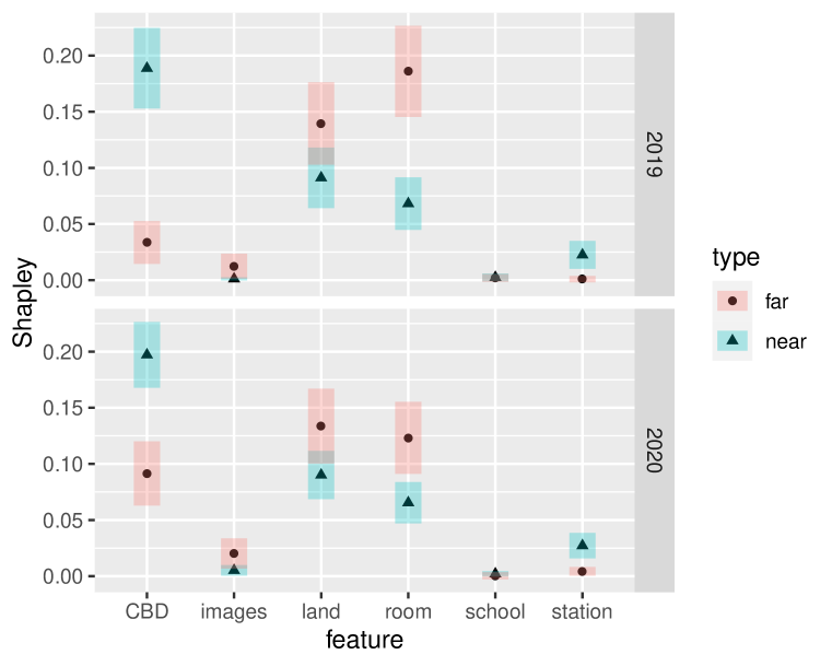
Figure 9: Shapley values and associated asymptotic 95% confidence intervals for each of the 6 covariates, within the 4 real estate data subgroups (near/far and 2019/2020). Blue bands and triangle markers represent the near subgroup (i.e., $\leq 25$km from Central Business District) and red bands with circular markers represent the far subgroup ($>25$km).

Table 3: Shapley values and asymptotic CIs for the covariates of the real estate data.

Feature	near (2019)	far (2019)	near (2020)	far (2020)
CBD	0.19 (-0.15,0.23)	0.03 (-0.02,0.05)	0.20 (-0.17,0.23)	0.10 (-0.06,0.12)
images	0.00 (-0.00,0.00)	0.01 ( 0.00,0.02)	0.06 ( 0.00,0.01)	0.02 ( 0.01,0.03)
land	0.09 ( 0.06,0.12)	0.14 ( 0.10,0.18)	0.09 ( 0.07,0.11)	0.13 ( 0.10,0.17)
school	0.00 (-0.00,0.00)	0.00 (-0.01,0.01)	0.00 (-0.00,0.00)	0.00 (-0.00,0.00)
station	0.02 ( 0.01,0.04)	0.00 (-0.00,0.00)	0.03 ( 0.02,0.04)	0.00 ( 0.00,0.01)
room	0.07 ( 0.05,0.09)	0.19 ( 0.15,0.23)	0.07 ( 0.05,0.08)	0.12 ( 0.09,0.16)

5 Discussion

In Section 2, we showed that under an elliptical (or pseudo-elliptical) joint distribution assumption, the game theoretic Shapley value decomposition of $R^{2}(\mathcal{Z}_{n})$ is asymptotically normal. Implementing this result, we produced asymptotic Shapley value CIs and hypothesis tests.

In Section 3, we examined the coverage and width statistics of these asymptotic CIs over a range of sample sizes, using Monte Carlo simulations. These simulations were conducted across three separate data generating processes: using a variety of correlations with a compound symmetry covariance matrix under multivariate normal (i) and Student-$t$ (ii) distributions. The simulations were also conducted under a normal distribution data generating process, with random Wishart covariance matrix (iii). In all three cases, the coverage and width statistics were compared to the corresponding statistics for the non-parametric bootstrap CIs. The computation time and memory usage were also benchmarked against the bootstrap CIs. In Section 3.5 we provided recommendations for when asymptotic CIs should be preferred and used, over the bootstrap CIs. We found that the asymptotic CIs have estimated coverage probabilities of at least $0.85$ across all studies, are preferable over the bootstrap CIs for small sample sizes ($n\leq 50$), and are often (although not always) favourable for large sample sizes. The asymptotic CIs are also far more computationally efficient than bootstrap CIs (at least for the cases of three and five explanatory variables), and show improved coverage and width when correlation is further from $c=0.5$.

Finally, in Section 4, we demonstrated the application of our derived asymptotic CIs to a data set consisting in house prices from Melbourne, to investigate a period of altered consumer behaviour during the initial stages of the arrival of COVID-19 in Australia. Using the CIs, we identified significant changes in model behaviour between 2019 and 2020, and attributed these changes amongst features, highlighting a potentially interesting direction of future research into the period. We also observed significant changes in behaviour between houses classified as close to the city, and those far from the city.

We have made the computational implementations of our methods openly available for use. These computational resources are implemented in the R and Julia programming languages.

We are preparing R, Julia, and Python versions of our methods for release. Our code and future progress regarding these implementations will be made available at github.com/BSMLcode/shapley_confidence. Additionally, we aim to use what we have developed in order to derive the asymptotic distributions of variance inflation factors and their generalizations [Fox and Monette, 1992], as well as the closely related Owen values decomposition of the coefficient of determination [Huettner and Sunder, 2012].

Appendix A Additional figures

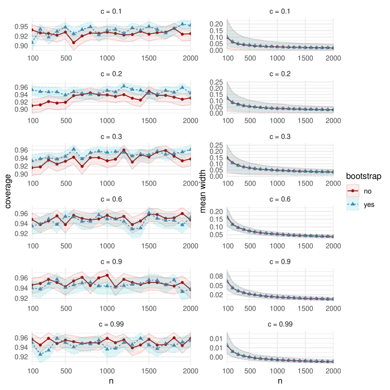
Figure 15: Comparisons of coverage (left column) and mean width (right column), between the bootstrap CIs (dashed lines with triangular markers) and the asymptotic CIs (solid lines with circular markers) in MC Study C. Rows represent correlations $c$, increasing from $0.1$ on the top row to $0.99$ on the bottom row. The horizontal axes display the sample sizes $n=100,200,\ldots,2000$.

References

- [Baglivo, 2005] Baglivo, J. A. (2005). Mathematica laboratories for mathematical statistics: emphasizing simulation and computer intensive methods. SIAM, Philadelphia.
- [Clopper and Pearson, 1934] Clopper, C. J. and Pearson, E. S. (1934). The use of confidence or fiducial limits illustrated in the case of the binomial. Biometrika, 26(4):404–413.
- [Cowden, 1952] Cowden, D. J. (1952). The multiple-partial correlation coefficient. Journal of the American Statistical Association, 47:442–456.
- [Efron, 1988] Efron, B. (1988). Computer-intensive methods in statistical regression. SIAM Review, 30:421–449.
- [Fang et al., 1990] Fang, K. T., Kotz, S., and Ng, K. W. (1990). Symmetric Multivariate and Related Distributions. Chapman and Hall.
- [Feltkamp, 1995] Feltkamp, V. (1995). Alternative axiomatic characterizations of the shapley and banzhaf values. International Journal of Game Theory, 24(2):179–186.
- [Fox and Monette, 1992] Fox, J. and Monette, G. (1992). Generalized collinearity diagnostics. Journal of the American Statistical Association, 87(417):178–183.
- [Fujikoshi et al., 2011] Fujikoshi, Y., Ulyanov, V. V., and Shimizu, R. (2011). Multivariate statistics: High-dimensional and large-sample approximations, volume 760. John Wiley & Sons.
- [Genizi, 1993] Genizi, A. (1993). Decomposition of in multiple regression with correlated regressors. Statistica Sinica, pages 407–420.
- [Greene, 2007] Greene, W. H. (2007). Econometric Analysis. Prentice Hall, New Jersey.
- [Gromping, 2006] Gromping, U. (2006). Relative importance for linear regression R: the package relaimpo. Journal of Statistical Software, 17:1–27.
- [Gromping, 2007] Gromping, U. (2007). Estimators of relative importance in linear regression based on variance decomposition. American Statistician, 61:139–147.
- [Hart et al., 1988] Hart, S., Mas-Colell, A., et al. (1988). The potential of the shapley value. the Shapley value, pages 127–137.
- [Hedges and Olkin, 1983a] Hedges, L. V. and Olkin, I. (1983a). Joint Distribution of Some Indices Based on Correlation Coefficients. Technical Report MCS 81-04262, Stanford University.
- [Hedges and Olkin, 1983b] Hedges, L. V. and Olkin, I. (1983b). Joint distributions of some indices based on correlation coefficients. In Karlin, S., Amemiya, T., and Goodman, L. A., editors, Studies in Econometrics, Time Series, and Multivariate Analysis. Academic Press.
- [Huettner and Sunder, 2012] Huettner, F. and Sunder, M. (2012). Axiomatic arguments for decomposiing goodness of fit according to Shapley and Owen values. Electronic Journal of Statistics, 6:1239–1250.
- [Israeli, 2007] Israeli, O. (2007). A Shapley-based decomposition of the R-square of a linear regression. Journal of Economic Inequality, 5:199–212.
- [Kruskal, 1987] Kruskal, W. (1987). Relative importance by averaging over orderings. The American Statistician, 41:6–10.
- [Lipovetsky and Conklin, 2001] Lipovetsky, S. and Conklin, M. (2001). Analysis of regression in game theory approach. Applied Stochastic Models in Business and Industry, 17:319–330.
- [Mardia, 1970] Mardia, K. V. (1970). Measures of multivariate skewness and kurtosis with applications. Biometrika, 57:519–530.
- [Olkin and Finn, 1995] Olkin, I. and Finn, J. D. (1995). Correlations redux. Quantitative Methods in Psychology, 118:155–164.
- [Seber, 2008] Seber, G. A. F. (2008). A Matrix Handbook For Statisticians. Wiley, New York.
- [Seber and Lee, 2003] Seber, G. A. F. and Lee, A. J. (2003). Linear Regression Analysis. Wiley, Hoboken.
- [Shapley, 1953] Shapley, L. S. (1953). A value for -person games. In Kuhn, H. W. and Tucker, A. W., editors, Contributions to the Theory of Games. Princeton University Press, Princeton.
- [Steiger and Browne, 1984] Steiger, J. H. and Browne, M. W. (1984). The comparison of interdependent correlations between optimal linear composites. Psychometrika, 49:11–24.
- [van der Vaart, 1998] van der Vaart, A. (1998). Asymptotic Statistics. Cambridge University Press, Cambridge.
- [Yeo and Johnson, 2000] Yeo, I.-K. and Johnson, R. A. (2000). A new family of power transformations to improve normality or symmetry. Biometrika, 87(4):954–959.
- [Young, 1985] Young, H. P. (1985). Monotonic solutions of cooperative games. International Journal of Game Theory, 14:65–72.
- [Yuan and Bentler, 1999] Yuan, K.-H. and Bentler, P. M. (1999). On normal theory and associated test statistics in covariance structure analysis under two classes of nonnormal distributions. Statistica Sinica, 9:831–853.
- [Yuan and Bentler, 2000] Yuan, K.-H. and Bentler, P. M. (2000). Inferences on correlation coefficients in some classes of nonnormal distributions. Journal of Multivariate Analysis, 72:230–248.