On the Length of Monotone Paths in Polyhedra

Abstract

Motivated by the problem of bounding the number of iterations of the Simplex algorithm we investigate the possible lengths of monotone paths followed by the Simplex method inside the oriented graphs of polyhedra (oriented by the objective function). We consider both the shortest and the longest monotone paths and estimate the monotone diameter and height of polyhedra. Our analysis applies to transportation polytopes, matroid polytopes, matching polytopes, shortest-path polytopes, and the TSP, among others.

We begin by showing that combinatorial cubes have monotone and Bland pivot height bounded by their dimension and that in fact all monotone paths of zonotopes are no larger than the number of edge directions of the zonotope. We later use this to show that several polytopes have polynomial-size pivot height, for all pivot rules. In contrast, we show that many well-known combinatorial polytopes have exponentially-long monotone paths. Surprisingly, for some famous pivot rules, e.g., greatest improvement and steepest edge, these same polytopes have polynomial-size simplex paths.

1 Introduction

It is a famous open challenge to find a pivot rule that can make the Simplex method run in polynomial time for all LPs or show that none exist (see e.g., [33, 5, 1] and the many references therein for a discussion of this famous algorithmic problem). In particular, such a pivot rule will take polynomially many monotonically-improving edge steps from any initial vertex. This paper discusses the possible lengths of the paths followed by the Simplex method on several famous combinatorial polyhedra where computing monotone paths has nice combinatorial meaning.

In what follows we consider a polytope/polyhedron $P(A,b)$ in the canonical forms $\{x\in\mathbb{R}^{n}:Ax=b,x\geq 0\}$ or $\{x\in\mathbb{R}^{n}:Ax\leq b,x\geq 0\}$. Here $A\in\mathbb{R}^{m\times n}$ and $b\in\mathbb{R}^{m}$. Objective function vectors will be typically denoted by $c\in\mathbb{R}^{n}$. $LP(A,b,c)$ will denote the (minimization) LP instance given by $A,b,c$. Given any $A,b,c$ such that $c$ is a nondegenerate linear objective function i.e., no two vertices have the same objective function, one has a natural directed acyclic graph on the vertices and edges of the polytope $P(A,b)$ by orienting each edge of the polytope $P(A,b)$ as per the objective value of the two endpoints. This will be denoted by $G(A,b,c)$. This kind of orientations of the graphs of $P(A,b)$ are called LP-admissible. We note that the directed graph $G(A,b,c)$ is always acyclic, with a unique sink and source in each face. While there is a characterization of the LP-admissible orientations for $3$-polytopes (see [21]), a similar result in higher dimensions seems unlikely (see [9]).

We introduce now the main combinatorial definitions and then give several remarks about these concepts. See Figure 1 for an example.

Definition 1.1.

Let $c$ be a linear objective function and $\pi$ a pivot rule.

1. A $c$-monotone path is a directed path in the LP-admissible oriented graph $G(A,b,c)$, that starts from some vertex to the optimal vertex (note that we always consider the optimal vertex to be the terminal node of the path, but we do not start necessarily at a specific node).

2. From each vertex there is at least one shortest $c$-monotone path to the optimum. The $c$-monotone diameter is the maximum length of a shortest $c$-monotone path, the maximum being taken over all starting vertices.

3. The $c$-height is the length of the longest $c$-monotone path.

4. A $c$-$\pi$-simplex path is a $c$-monotone path in $G(A,b,c)$ following the pivot rule $\pi$. In this paper we will consider four popular pivot rules: Bland’s pivot rule, Dantzig’s pivot rule, greatest improvement pivot rule, and steepest edge pivot rule.

We use these definitions to build our main concepts of interest.

Definition 1.2.

1. The monotone diameter of a polytope is the maximum $c$-monotone diameter, the maximum being taken over all objective functions $c$.

2. The height is the maximum $c$-height, the maximum being taken over all objective functions $c$.

3. The $\pi$-pivot height is the maximum length of a $c$-$\pi$-simplex path for the pivot rule $\pi$, the maximum being taken over all objective functions $c$.

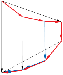
Figure 1: Two monotone paths on the directed graph $G(A,b,c)$ of the Klee$-$Minty cube. The longest monotone path in red gives the height and the blue monotone path gives the monotone diameter of this polytope.

The study of the undirected diameter of the graph of polytopes is of course classical and related to the Hirsch conjecture (see e.g., [30] and references), but the investigations of directed monotone paths are even more directly relevant to the Simplex method, and they have occupied researchers for some time: In the 1960’s Klee initiated the study of short/long monotone paths in his papers [18, 17] where he proved bounds on the monotone diameter and height of simple polytopes. Later in the 1980’s, in a remarkable tour de force, Todd [32] showed that the monotone Hirsch conjecture, saying that the monotone diameter is always less or equal to the number of facets minus the dimension, is false. In the 1990’s Kalai [14] proved that for a $n$-dimensional polyhedron with $m$ facets there is a subexponential bound on the monotone diameter of $m^{2\sqrt{m}}$. Today, several papers continue the study of shortest monotone paths (see [12] and references therein).

It must be noted that there are several exponentially-long $c$-$\pi$-simplex paths, e.g., the Klee-Minty cubes [19] and similar counterexamples for other pivot rules (see discussion and references in [5]). The notion of height is useful to indicate the worst possible case of the Simplex method. In fact, long monotone paths have also been explored before, the monotone upper bound problem asks for the maximal number $M(n,m)$ of vertices on a strictly increasing edge-path on a simple $n$-dimensional polytope with $m$ facets. This is the same as the largest height over all simple $n$-polytopes with $m$ facets. It was conjectured that $M(n,m)$ is never more than the number of vertices of a dual-to-cyclic $n$-polytope with $m$ facets, but proven to be strictly less than that in dimension six [25]. In our paper the reader can observe how the bound $M(n,m)$ is often too big for specific polytopes. In fact, Del Pia and Michini [8] recently proved that for lattice polyopes contained in $[0,k]^{n}$, there exists a pivot rule $\pi$ for which the $\pi$-pivot height is at most $O(n^{6}k\log n)$.

We wish to stress that computational complexity influences the geometry of monotone paths of polytopes. In [1] it was shown that there are Simplex pivoting rules for which it is PSPACE-complete to decide whether a particular basis will appear on the algorithm’s path. This happens even for the Dantzig pivot rule [11]. Moreover, it was recently shown in [6] that it is hard to compute the monotone diameter. It is also difficult to decide when a monotone path is a simplex path but we focus here on four well-known pivot rules: Bland’s pivot rule, Dantzig’s pivot rule, greatest improvement pivot rule, and steepest edge pivot rule.

Finally the concepts we discuss in this paper satisfy the following relation:

$$\text{\em(undirected) diameter}\leq\text{\em monotone diameter}\leq\pi\text{\em-pivot height}\leq\text{\em height}.$$

We now summarize our main results about these concepts.

Our results

In Section 2 we show that combinatorial cubes have monotone and Bland pivot height bounded by their dimension. Similarly, zonotopes have height never larger than the number of edge directions of the zonotope.

Theorem 1.3.

Let $P$ be a convex polytope. Denote by $Z(P)$ the zonotope generated by $E$, the minimal set of vectors containing all directions of edges of $P$. $\text{mono-diam}(P)\leq\text{mono-diam}(Z(P))=\text{number of different edge directions of }P$.

This simple theorem has nice consequences. We can easily show that matroid polytopes, polymatroid polytopes, and some types of transportation polytopes have polynomial-size height and pivot height for all pivot rules.

Corollary 1.4.

If $P$ is a matroid polytope or a polymatroid polytope, then $\text{mono-diam}(P)\leq{\binom{n}{2}}$, where $n$ is the number of elements of the matroid.

This follows immediately from the bounds on the number of edge directions of a matroid or polymatroid polytope, see Theorem 5.1. in [34]. Therefore, polytopes such as the permutahedron or the spanning tree polytope behave particularly well in the Simplex method as all pivot rules are efficient. This is also true in other cases.

Theorem 1.5.

If $P$ is a $k\times n$ transportation polytope, $\text{mono-diam}(P)\leq e\cdot k!\,n^{k}$. Therefore, the monotone diameter of $k\times n$ transportation polytopes for fixed $k$ is polynomial in $n$.

In Section 3 we show that many well-known combinatorial polytopes have exponentially-long monotone paths, and thus exponential height.

Theorem 1.6.

The height of the matching, perfect matching, fractional matching and fractional perfect matching polytopes on the complete graph $K_{n}$ is $>C\cdot\lfloor\frac{n}{2}-1\rfloor!$ for a universal constant $C>0$.

Theorem 1.7.

There exist monotone paths of length $>C\cdot\phi^{n}$ on the perfect 2-matching polytope and on the TSP with $n$ nodes for a universal constant $C>0$ and $\phi=\frac{1+\sqrt{5}}{2}$ the golden ratio.

Theorem 1.8.

There exist monotone paths of length $>\frac{C}{n^{2}}\sqrt[3]{n!}$ on the shortest path polytope on the complete graph $K_{n}$ for some universal constant $C>0$.

In contrast, we prove that, for at least one of three famous pivot rules, Bland’s, greatest improvement and steepest edge, they have polynomial-size pivot height. Our discussion includes matching polytopes, fractional matching polytopes, shortest-path polytopes, and the TSP.

Theorem 1.9.

The number of vertices visited, by Dantzig or greatest improvement pivot rules paths, is bounded by

1. $m\left[n\log(2n)\right]$ for the fractional perfect matching polytope ($FPM$) on a graph with $n$ nodes and $m$ edges. For the complete graph $K_{n}$, we get a bound $\sim\frac{n^{3}}{2}\log n$.

2. $m\left[2n\log(2n)\right]$ for the fractional matching polytope ($FM$) on a graph with $n$ nodes and $m$ edges. For the complete graph $K_{n}$, we get a bound $\sim n^{3}\log n$.

3. $n^{2}\left[n\log(2n-1)\right]\sim n^{3}\log n$ for the Birkhoff polytope on the bipartite graph $K_{n,n}$.

4. $(n^{2}-2n+1)\left[(n-1)\log(n-1)\right]\sim n^{3}\log n$ for the shortest path polytope on $n$ nodes.

Theorem 1.10.

For the steepest-edge pivot rule paths, the number of visited vertices is bounded by

1. $m\left[2n\sqrt{n}\log(2n)\right]$ for the fractional perfect matching polytope ($FPM$) on a graph with $n$ nodes and $m$ edges. For the complete graph $K_{n}$, we get a bound $\sim n^{3}\sqrt{n}\log n$.

2. $m\left[4n\sqrt{2n}\log(2n)\right]$ for the fractional matching polytope ($FM$) on a graph with $n$ nodes and $m$ edges. For the complete graph $K_{n}$, we get a bound $\sim 2n^{3}\sqrt{2n}\log n$.

3. $n^{2}\left[n\sqrt{\frac{n}{2}}\log(2n-1)\right]\sim n^{3}\sqrt{\frac{n}{2}}\log n$ for the Birkhoff polytope.

4. $(n^{2}-2n+1)\left[(n-1)\sqrt{\frac{2n}{3}}\log(n-1)\right]\sim n^{3}\sqrt{\frac{2n}{3}}\log n$ for the shortest path polytope.

In Section 4 we consider again the problem of estimating the monotone diameter of transportation polytopes.

Theorem 1.11.

A $2\times n$ transportation polytope has monotone diameter $\leq n$. Therefore, $2\times n$ transportation problems satisfy the monotone Hirsch conjecture.

2 Monotone and Simplex paths on Cubes & Zonotopes

In this section we present several results about monotone paths and simplex paths on cubes and zonotopes. We will see they have more general applicability.

Theorem 2.1.

Let $C\subset\mathbb{R}^{n}$ be a polytope combinatorially equivalent to a hypercube. Then $\text{mono-diam}(C)=n$. Furthermore, there exists an ordering of the facets of $C$ such that Bland’s pivot rule reaches the optimal solution in at most $n$ steps for any initial vertex.

Proof.

We first prove by induction on $n$ that the monotone diameter is $n$. For $n=1$, the result is trivial. Assume now that the result is true for any combinatorial cube up to dimension $n-1$. Consider an arbitrary vertex $x\neq x^{*}$ of $C$. There must exist an improving edge going out of $x$. Consider a facet $F$ containing $x$ but that does not contain this edge. If $x^{*}\in F$, we are done by the induction hypothesis. Otherwise $x^{*}$ belongs to the “opposite” facet. This is the facet of the polytope which does not have any vertex in common with the facet $F$. For example if $C$ is the regular hypercube, this is the parallel facet to $F$. We take the improving edge to that opposite facet and apply the induction hypothesis. To conclude note that the monotone diameter is exactly $n$ because there exists a vertex which needs at least $n$ pivots to reach the optimal solution.

Now let us present good orderings of the facets for Bland’s pivot rule. Denote by $x^{*}$ the optimum vertex. We choose an ordering such that the first $n$ facets satisfy $x^{*}\notin F_{i}$ for $1\leq i\leq n$ and the last $n$ facets satisfy $x^{*}\in F_{i}$ for $n+1\leq i\leq 2n$. We will prove that Bland’s rule with this ordering follows the path described above. More precisely, we prove that at each step, the index of the entering variable is in $\{1,\ldots,n\}$ while the index of the leaving variable is in $\{n+1,\ldots,2n\}$ so inserted variables will never be removed from the basis.

Consider an arbitrary vertex $x\neq x^{*}$. Let $i_{1},\ldots,i_{k}>n$ be the indices such that $x\in F_{i}$. Since $x$ is not the optimum, there must exist an improving edge from $x$ in the cube $F_{i_{1}}\cap\ldots\cap F_{i_{k}}$ of smaller dimension $n-k$. Consider the facet $F_{i}$ of the $n$-dimensional cube such that $x\in F_{i}$ and that does not contain this improving edge. Note that $i\leq n$. Otherwise $x^{*}\in F_{i}$, therefore $F_{i}$ is one of the facets $F_{i_{1}},\ldots,F_{i_{k}}$ which is impossible because the improving edge is contained in their intersection.

The entering variable $\hat{i}$ chosen by Bland’s pivot rule satisfies $\hat{i}\leq i\leq n$. Note that $x^{*}\notin F_{\hat{i}}$ so $x^{*}$ is contained in the “opposite” facet which corresponds to the leaving variable. Therefore the index of the leaving variable is greater than $n$. Then, variables of index $\leq n$ cannot be removed from the basis. ∎

Note that these good orderings of the facets for Bland’s pivot rule are very rare. Since the $n$ facets not containing the optimum should have the first $n$ indices in the ordering while the $n$ facets containing the optimum should have the last $n$ indices, there are $(n!)^{2}$ such good orderings among the $(2n)!$ possible orderings of the facets. Therefore, the proportion of good orderings for Bland’s pivot rule is $\frac{1}{\binom{2n}{n}}$.

Next, we discuss the monotone diameter of another family of polytopes: zonotopes. A zonotope is the Minkowski sum of a set of line segments.

Lemma 2.2.

Let $Z(v^{1},\ldots,v^{m})\subset\mathbb{R}^{n}$ be the zonotope generated by those directions. Assume any two directions $v^{i},v^{j}$ are non-colinear. In at most $m$ augmenting steps, one can go from $\hat{x}$, an initial vertex, to $x^{*}$ the optimum. This bound is tight. Furthermore, any monotone path has at most $m$ steps so any pivot rule will take at most $m$ steps to the optimum.

Proof.

Let $c\in\mathbb{R}^{n}$. We define $J^{+}=\{j\mid c^{T}v^{j}>0\}$ and $J^{-}=\{j\mid c^{T}v^{j}<0\}.$ Observe that $x^{*}=\sum_{j\in J^{-}}v^{j}$. Consider a starting point $\hat{x}$. We can write it as $\hat{x}=\sum_{j\in S(\hat{x})}v^{j}$ for a certain subset $S(\hat{x})\subset\{1,\ldots,m\}$.

Two adjacent vertices of the zonotope differ by $\pm v^{i}$ for some $i$. Then, the only edges a monotone path can use are $\varepsilon_{i}v^{i}$ where $\varepsilon_{i}=1$ if $i\in J^{-}$ and $\varepsilon_{i}=-1$ if $i\in J^{+}$. Furthermore, the path can follow each of these directions at most once because once $\varepsilon_{i}v^{i}$ is added, this term cannot be removed by the other possible directions. Then, the length of the path is at most $m$.

Furthermore, since the admissible edges are of the form $\varepsilon_{i}v^{i}$, the point $\tilde{x}=\sum_{j\in J^{+}}v^{j}$ is at distance at least $m$ from the optimum. Note that $\tilde{x}$ is a true vertex of the zonotope because it is the optimum for the cost function $-c$. ∎

Lemma 2.3.

Let $Z(v^{1},\ldots,v^{m})\subset\mathbb{R}^{n}$ be a zonotope. Assume any pair of directions $v^{i},v^{j}$ are non-colinear. It has at least $2m$ facets.

Proof.

Let $v^{i_{1}},\ldots,v^{i_{d-1}}$ be a linearly independent subset of size $n-1$. Then $Z(v^{1},\ldots,v^{m})$ has two facets that are translates of $Z(v^{i_{1}},\ldots,v^{i_{d-1}})$. This is because for an objective function $c\in\ker([v^{i_{1}},\ldots,v^{i_{d-1}}])$ the optimum facet of $Z(v^{1},\ldots,v^{m})$ with respect to $\pm c$ are precisely these facets. It suffices to show that there are $\geq m$ distinct subsets of this type.

Without loss of generality, let $v^{1},\ldots,v^{n}$ be linearly independent.
$S^{i}=\{v^{1},\ldots,v^{i-1},v^{i+1},\ldots,v^{n}\}$, $i=1,\ldots,n$ are $n$ such subsets. For any $v^{j}$ with $j\geq n+1$, there exists $v\in\{v^{1},\ldots,v^{n}\}$ such that $\{v^{1},\ldots,v^{n}\}\setminus\{v\}\cup\{v^{j}\}$ is linearly independent (by the matroid axiom). Therefore drop $v$ and add $v^{j}$, the corresponding subset gives two more facets. We get $m-n$ additional subsets like this. ∎

The following theorem shows that zonotopes satisfy the monotone Hirsch conjecture.

Theorem 2.4.

$\text{mono-diam}(Z(v^{1},\ldots,v^{m}))=m\leq\frac{|\text{facets}|}{2}\leq|\text{facets}|-n$.

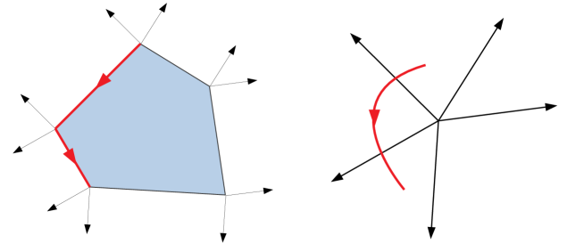
Figure 2: Left, a path on a polytope and right, the corresponding path on the normal fan.

We will now use this result to bound the monotone diameter of general polytopes. For this, let us define the normal cone of a vertex $v$ as the set of objective vectors $c$ such that $v$ is the optimum vertex for the corresponding objective function, and the normal fan as the collection of normal cones for all vertices of the polytope (see [3] and Figure 2 for an illustration).

Lemma 2.5.

(Gritzmann-Sturmfels, Proposition 2.1.8. in [13]) Let $P\subset\mathbb{R}^{n}$ be a polytope and let $E$ be a finite set of vectors containing all the direction of edges of $P$. of $P$. The normal fan of the zonotope generated by $E$ is a refinement of the normal fan of $P$, therefore the length of the shortest paths in $Z(E)$ upper bound the length of the shortest paths in $P$.

Proof of Theorem 1.3.

The first inequality of the theorem follows from Lemma 2.5 because we view a path on the graph of the polytope as a sequence of normal fans where consecutive normal fans share a facet. The normal to this shared facet is the direction of the corresponding edge between the two vertices on the graph of the polytope. Therefore any monotone path $p$ on the zonotope for the linear function $c$ leads to a path $\tilde{p}$ with smaller length on the original polytope. $\tilde{p}$ is still monotone for $c$ because the directions of the edges of $\tilde{p}$ are contained in the directions of the edges of $p$ according to Lemma 2.5. ∎

We can now apply Lemma 1.3 to several polytopes. The essential message is that if the set of edge-directions is “small” or polynomially bounded, then we can obtain a bound on the height using the above result. While we show some nice situations below, in most cases this is not useful (see [22] where a lower bound on the number of edge directions is discussed).

Proof of Theorem 1.5.

Edges on transportation polytopes are alternating sign cycles on the bipartite graph. Since there are $k$ supply nodes, the length of the cycle is $2p$ for $2\leq p\leq k$. The number of such cycles of length $2p$ is $\frac{1}{p}\frac{n!k!}{(n-p)!(k-p)!}$. Then, the number of different edge directions is bounded by

$$\sum_{p=2}^{k}\frac{1}{p}\frac{n^{p}k!}{(k-p)!}\leq n^{k}k!\sum_{p=2}^{k}\frac{1}{(k-p)!n^{k-p}}\leq e^{1/n}n^{k}k!$$

and the proof follows. ∎

Finally, the above family in Corollary 1.5 is naturally generalized by $N$-fold linear programs, see Chapter 4 in [7]. In that case the defining matrix $A$ has a very specific shape as multiple copies of smaller matrices. We omit details.

3 Monotone and Simplex paths on $0/1$ and $0/\frac{1}{2}/1$ polyhedra

In this section, we give results on the height, monotone diameter, and the pivot height of some well-known polytopes. It should be noted that the papers [16, 6] provide general polynomial bounds for $0/1$-polytopes and their monotone diameters are also polynomial. But in this section we look at specific families and thus we can obtain more precise polynomial bounds.

The height of a polytope $P$ is the length of the longest path in the directed graph of $P$. To start, note that the height gives a bound on the number of steps of the worst possible pivot rule of the Simplex algorithm. As shown in Section 2 for some particular polytopes (e.g., zonotopes) the height is polynomially bounded, thus it gives a polynomial bound for the Simplex algorithm for any pivot rule. However, it turns out that, for many polytopes of interest and for some well-known $0/1$ and $0/\frac{1}{2}/1$ polyhedra, monotone paths can be very long. Here we collect some of the results about the height of polyhedra:

First, Pak [24] showed that the height of the Birkhoff polytope is exponential.

Theorem 3.1 (Pak, Theorem 1.4. in [24]).

There exists a linear function $\phi$ with a decreasing sequence of vertices of length $>C\cdot n!$ of the Birkhoff polytope on the bipartite graph $K_{n,n}$ for a universal constant $C>0$.

Note that the graph of a face $F$ of a polytope $P$ is a proper subgraph of the graph of $P$. Therefore the height of a polytope is greater or equal to the height of any of its faces. Indeed, let $c$ be a cost function in $F$. For $P$ take that same cost function parallel to $F$ and denote it by $\tilde{c}$. Then any monotone path in $(F,c)$ is a monotone path in $(P,\tilde{c})$.

Let us recall the definitions and basic properties of the combinatorial polytopes we will consider in this Section. A matching in a graph $G=(V,E)$ is a subset of edges $M\subset E$ such that every vertex meets at most one edge of $M$. A matching is perfect if every vertex meets exactly one edge of $M$. The perfect matching polytope (M) of $G$ is defined as the convex hull of the $0/1$ incidence vectors of matchings i.e.,

$$\text{M(G)}=\text{conv}\{\chi^{M}:M\text{ is a matching of G}\}.$$

The perfect matching polytope (PM) of $G$ is the convex hull of the perfect matchings. Note that the perfect matching polytope on the complete bipartite graph is the Birkhoff polytope.

$$\text{PM(G)}=\text{conv}\{\chi^{M}:M\text{ is a perfect matching of G}\}$$

For these two polytopes, two matchings are adjacent if and only if the union of their support graph contains a unique cycle (see Lemma 1 in [26]). A set of inequalities describing these polytopes is given by the Edmond’s matching theorem [10].

We also consider the relaxations of these polytopes obtained by omitting the odd cycle inequalities. The fractional matching polytope (FM) of $G$ is defined by

$$\text{FM(G)}=\{x\in\mathbb{R}^{E}(G):\;x_{e}\geq 0\;\forall e\in E(G),\;x(\delta(v))\leq 1\;\forall v\in V(G)\}$$

where $E(G),V(G)$ of course denote, respectively, the sets of edges and vertices of the graph $G$. Similarly, the fractional perfect matching (FPM) is described by

$$\text{FPM(G)}=\{x\in\mathbb{R}^{E}(G):\;x_{e}\geq 0\;\forall e\in E(G),\;x(\delta(v))=1\;\forall v\in V(G)\}.$$

Note that M(G) and PM(G) are respectively a face of FM(G) and FPM(G). The adjacency of these fractional polytopes is given in Theorem 25 of [2]. In the following we will only use the fact that the graph of M(G) and PM(G) are, respectively, a subgraph of FM(G) and FPM(G).

A 2-matching of $G$ is a subset of edges $M$ such that every vertex is incident to exactly $2$ edges in $M$. Note that a 2-matching is the union of disjoint cycles. The perfect 2-matching polytope (P2M) of $G$ is defined as a $0/1$ polytope as follows,

$$\text{P2M(G)}=\text{conv}\{\chi^{M}:M\text{ is a perfect 2-matching of G}\}.$$

Two 2-perfect matchings are adjacent if and only if the symmetric difference of their support graphs contains a unique alternating cycle (see Lemma 1 in [27] and Figure 3 for an illustration).

In the following, if the graph is not specified we will consider the complete graph $K_{n}$.

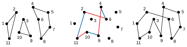
Figure 3: Left and right, two adjacent perfect 2-matchings. In the middle, the corresponding alternating cycle.

The traveling salesman polytope (TSP) on $K_{n}$ is the convex hull of tours i.e., cycles of length $n$. The TSP graph is therefore a proper subgraph of the perfect 2-matching polytope of $K_{n}$ (see [29]).

Finally, the shortest path polytope on $n$ nodes is defined as the convex hull of paths from say node $1$ to node $n$ without cycles. A system of equations is given by

$$\left\{(x_{i,j}\geq 0)_{1\leq i\leq n-1,\ 2\leq j\leq n}:\,\sum_{j=2}^{n}x_{1,j}=1,\sum_{j\neq i}x_{i,j}-\sum_{j\neq i}x_{j,i}=0,\sum_{j\neq i}x_{i,j}\leq 1,\,2\leq i\leq n-1\right\}.$$

Two paths are adjacent if and only if the union of their support graph contains a unique cycle (see Lemma 2 in [26]).

Proof of Theorem 1.6.

We show that the Birkhoff polytope is a face of each of the considered polytopes. We will denote by $x_{i,j}$ the component corresponding to the edge between nodes $i$ and $j$ for a vertex $x$ in the polytope. Note that graphs are non-oriented here.

Define $E_{1}:=\{1,\ldots,\lfloor\frac{n}{2}\rfloor\}$ and $E_{2}:=\{\lfloor\frac{n}{2}\rfloor+1,\ldots,2\lfloor\frac{n}{2}\rfloor\}$. For the matching polytope and the fractional matching polytope, the corresponding face can be described by the several equalities $x_{i,j}=0$ for $(i,j)\notin E_{1}\times E_{2}\cup E_{2}\times E_{1}$ and $x(\delta(i))=1$ for $i\in E_{1}\cup E_{2}$. In both the matching and fractional matching polytopes, these equalities describe the set of perfect matchings on the bipartite graph between $E_{1}$ and $E_{2}$ i.e., vertices of these facets are in exact correspondence with the vertices of the $K_{E_{1},E_{2}}$ Birkhoff polytope. Furthermore, the adjacency between the perfect matchings of these faces is exactly the same as in the Birkhoff polytope. Hence the corresponding face is equivalent to the Birkhoff polytope with $2\times\lfloor\frac{n}{2}\rfloor$ nodes. The monotone diameter of these polytopes is therefore greater than the bound $C\lfloor\frac{n}{2}\rfloor!$ given in Theorem 3.1.

For the perfect matching polytope we can simply take the equalities $x_{i,j}=0$ for $(i,j)\notin E_{1}\times E_{2}\cup E_{2}\times E_{1}$. The other equalities of the form $x(\delta(i))$ are already satisfied. We get the same bound $C\lfloor\frac{n}{2}\rfloor!$ for the monotone diameter.

The same argument holds for the fractional perfect matching polytope when $n$ is even. However, when $n$ is odd, matchings on $K_{E_{1},E_{2}}$ are not vertices of the polytope anymore. In this case, we can restrict to the face $x_{n-2,n-1}=x_{n-1,n}=x_{n-2,n}=1/2$ and use the same arguments as above with $E_{1}:=\{1,\ldots,\frac{n-3}{2}\}$ and $E_{2}:=\{\frac{n-1}{2},\ldots,n-3\}$. We finally get the bound $C\lfloor\frac{n}{2}-1\rfloor!$ for the monotone diameter. ∎

Proof of Theorem 1.7.

Recall that $n$-tours, which are the vertices of the TSP, are also vertices of the perfect 2-matching polytope. If two tours are adjacent on the perfect 2-matching polytope, then they are also adjacent in TSP (see [29]). Therefore it suffices to prove that there exists a long monotone path on the perfect 2-matching polytope going through $n$-tours only.

Denote by $x_{i,j}$ the component corresponding to the edge between nodes $i$ and $j$ for a vertex $x$ in the polytope. Consider the following linear function:

$$\psi=x_{1,2}+\alpha x_{1,3}+\ldots+\alpha^{n-2}x_{1,n}+\alpha^{n-1}x_{2,3}+\alpha^{n}x_{2,4}+\ldots+\alpha^{\frac{n(n-1)}{2}-1}x_{n-1,n}$$

for $0<\alpha<1/2$ such that the linear order on the perfect 2-matching polytope or on the TSP is the lexicographic order on the edges with the following order:

$\{1,2\},\{1,3\},\ldots,\{1,n\},\{2,3\},\ldots,\{n-1,n\}$.

Denote by $x^{*}=(1,n,2,n-1,3,n-2,\cdots)$ the optimum for TSP, see Figure 5e). The initial tour is going to be the cycle $x^{0}=(1,2,\ldots,n)$. We will construct by induction a monotone path with exponential length. We denote by $L_{n}$ the length of this monotone path. For $n\geq 4$, assume that we have constructed these long monotone paths for $k=4,\cdots,n-1$. Let us now construct the path of length $L_{n}$.

Step 1: We first restrict to $x_{1,2}=1$. We can get to the optimum $x^{1}$ of this facet in at least $L_{n-1}$ steps. Indeed if $x$ is a $(n-1)$-tour in the long path for $n-1$ nodes, define $\tilde{x}$ a $n$-tour by dividing node $1$ into two nodes $1$ and $2$. The indices of the other nodes should be shifted by one accordingly. Recall that two 2-matchings are adjacent if and only if the symmetric difference of their edges defines a unique alternating cycle. Let $x_{1}$ and $x_{2}$ be two adjacent tours in the $(n-1)$-perfect 2-matching. Then either $\tilde{x}_{1}$ and $\tilde{x}_{2}$ are adjacent in the $n$-perfect 2-matching or $\tilde{x}_{1}$ and $\hat{x}_{2}$ are adjacent where $\hat{x}_{2}$ is the same tour as $\tilde{x}_{2}$ except the two nodes coming from the division of node $1$ have been switched. We can therefore construct a path of length $L_{n-1}$ corresponding to the same path for $(n-1)$-tours. We then get from the corresponding end point to the optimum of the facet $x_{1,2}=1$ (see Figure 5a)). These two tours might be distinct if we have to switch the two nodes coming from the division of node $1$, which takes at most one step.

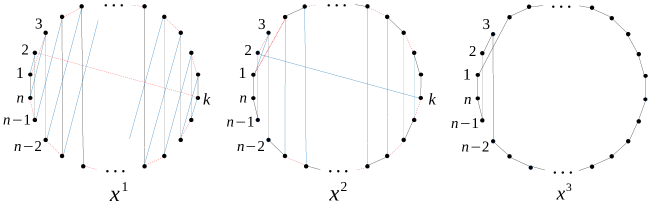
Figure 4: Step 2 of the monotone path on TSP. Edges in blue are the edges going to be deleted and the dashed red edges are going to be inserted. Since they form an alternating cycle, these tours are adjacent.

Step 2: We now get in two improving steps to the tour $x^{3}=(1,4,5,\ldots,n-2,3,2,n-1,n)$ (see Figure 4). The edges of the current vertex $x^{1}$ are $x^{1}_{i,n+1-i}=1$ for all $i$, $x^{1}_{1,2}=x^{1}_{i,n+3-i}=1$ for $i\geq 3$. We now get to the tour $x^{2}=(2,n-1,n,1,3,n-2,n-3,4,5,\ldots,k)$ which uses all the edges of the form $x_{i,n+1-i}$. Here $k=\frac{n}{2}+1$ if $n\equiv 0\mod 4$, $k=\frac{n}{2}$ if $n\equiv 2\mod 4$ and $k=\frac{n+1}{2}$ otherwise. This is an adjacent node because the symmetric difference of the graphs of the two tours has a unique alternating cycle $(2,1,3,n,n-1,4,5,n-2,n-3,6,7,\ldots k)$. The precise end of this alternating cycle depends on $n\mod 4$. If $n\equiv 0\mod 4$, the ending of this cycle is $(\ldots,k-2,k-1,k+2,k+1,k)$. If $n\equiv 2\mod 4$, it is $(\ldots,k-2,k-1,k+4,k+3,k)$. For $n\equiv 1\mod 4$, it is $(\ldots,k-2,k+4,k+3,k-1,k,k+2,k+1,k)$ and for $n\equiv 3\mod 4$ it is $(\ldots,k+2,k+1,k+3,k+2,k)$. Because $x^{2}_{1,2}=0$, this is an improving step for the lexicographic order on the edges. Now use the alternating cycle $(2,3,1,4,n-3,n-4,5,6,n-5,n-6,\ldots,k)$ to get to the neighbor tour $x^{3}=(1,4,5,\ldots,n-2,3,2,n-1,n)$. More precisely, the ending of the alternating cycle is $(\ldots,k-3,k-2,k+1,k)$ if $n\equiv 0\mod 4$, $(\ldots,k-2,k+3,k+2,k-1,k)$ if $n\equiv 2\mod 4$, $(\ldots,k-2,k-1,k+1,k)$ if $n\equiv 1\mod 4$ and $(\ldots,k-2,k+2,k+1,k-1,k)$ if $n\equiv 3\mod 4$. This is also an improving step because $x_{1,2}^{3}=x_{1,3}^{3}=0$.

Now we fix $x_{n-1,2}=x_{2,3}=x_{3,n-2}=1$. We get to optimal tour of this facet (see Figure 5b)) in at least $L_{n-3}$ steps, similarly to the technique used for the $L_{n-1}$ long step: in the $n$-tour, nodes $n-1,2,3$ and $n-2$ will be merged together to obtain a $(n-3)$-tour.

Step 3: Note that now $\{1,n\}$ and $\{1,n-1\}$ are edges that will never be removed so we are restricted to the facet $x_{1,n}=x_{1,n-1}=1$. Merging together nodes $1,n,n-1$, the resulting $(n-2)$-tour is exactly the tour given at the end of step 1 for $n-2$ nodes. Apply Step 2 again to get to the next tour in at least $2+L_{n-5}$ steps which is the optimum of the facet $x_{1,n}=x_{1,n-1}=x_{n-2,3}=x_{3,4}=x_{4,n-3}=1$ (see Figure 5c)). Now, $\{2,n\}$ and $\{2,n-2\}$ are edges that will never be removed so we are restricted to the facet $x_{2,n}=x_{2,n-2}=1$. With the same arguments, we progressively reconstruct the edges of the optimum $x^{*}$ in at least $2+L_{n-7}+2+L_{n-9}+\ldots$ steps.

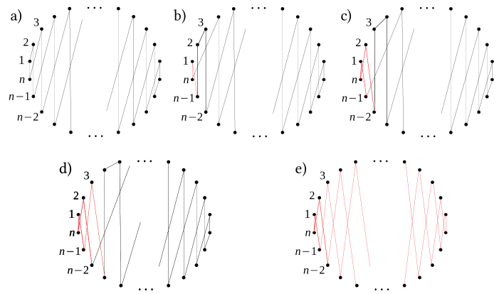
Figure 5: Main steps of the monotone path. Once the red edges that belong to the optimum $e)$ are inserted they will never be deleted.

Together, we have $L_{n}\geq L_{n-1}+2+L_{n-3}+2+L_{n-5}+\ldots+2+L_{k}$ with $k=4$ if $n$ is odd and $k=5$ otherwise. Define $\tilde{L}_{n}$ by $\tilde{L}_{4}=1$, $\tilde{L}_{5}=3$ and $\tilde{L}_{n}=\tilde{L}_{n-1}+2+\tilde{L}_{n-3}+2+\tilde{L}_{n-5}+\ldots+2+\tilde{L}_{k}$. Then $L_{n}\geq\tilde{L}_{n}$ because $L_{4}\geq 1$ and $L_{5}\geq 3$. Furthermore, $\tilde{L}_{n}=\tilde{L}_{n-1}+\tilde{L}_{n-2}+2$ therefore note that $\tilde{L}_{n}+2=F_{n}$ is the Fibonacci sequence. Then $L_{n}\geq\tilde{L}_{n}\geq\frac{\phi^{n}}{\sqrt{5}}-3$. ∎

Proof of Theorem 1.8.

Recall that the vertices of the shortest path polytope are the paths from node say $1$ to $n$ (all nodes of the path should be distinct) and that two paths from $1$ to $n$ are adjacent if and only if the union of their graphs forms a unique cycle. Denote by $x_{i,j}$ the coordinate of the edge going from node $i\neq n$ to $j\neq 1$ in a vertex $x$ of the polytope. Similarly to the cost function used in Theorem 1.7 we use the linear function

$$\psi=x_{1,2}+\alpha x_{1,3}+\ldots+\alpha^{n-2}x_{1,n}+\alpha^{n-1}x_{2,3}+\ldots+\alpha^{2n-4}x_{2,n}+\ldots+\alpha^{n^{2}-3n+2}x_{n-1,n},$$

so that the linear order is the lexicographic order on the edges
$\{1,2\},\{1,3\},\ldots,\{1,n\},\{2,3\},\ldots,\{2,n\},\{3,2\},\{3,4\},\ldots,\{3,n\},\ldots,\{n-1,n\}$ with a chosen small enough $\alpha>0$. We start from the path $1,2,\ldots,n$ which is the maximum value vertex for $\psi$. Denote by $L_{n}$ the length of the monotone path we will construct here by induction.

Step 1: Fix the edge $x_{1,2}=1$. This facet corresponds to the shortest path polytope on the complete graph $K_{n-1}$ with nodes $2,3,\ldots,n$. The objective function $\psi$ is still the same lexicographic order on the edges of $K_{n-1}$. Then, by induction, we can get to path $1,2,n$ in $L_{n-1}$ monotone steps.

Step 2: We now get to the path $1,3,4,\ldots,n$ which is a decreasing neighbor because we do not use the edge $\{1,2\}$ anymore. Similarly to Step 1, we get to path $1,3,n$ in $L_{n-2}$ monotone steps.

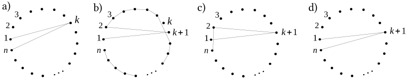
Figure 6: Step 3 of the long monotone path on the shortest path polytope. The length of the path from a) to d) is $L_{n-3}+2$.

Step 3: We are now going to go from path $1,3,n$ to $1,4,n$, then to $1,5,n$ etc… to $1,n-1,n$ (see Figure 6). From the path $1,k,n$ where $k\geq 3$ we get to the decreasing neighbor $1,k+1,2,3,\ldots,k-1,k+2,k+3,\ldots,n$ (see Figure 6 b)). Fixing edges $x_{1,k+1}=x_{k+1,2}=1$, this facet is equivalent to the shortest path on the complete graph $K_{n-3}$ with nodes $2,3,\ldots,k-1,k+2,k+3,\dots,n$, starting in $2$ and ending in $n$. We therefore get to path $1,k+1,2,n$ in $L_{n-3}$ steps and then to path $1,k+1,n$ in an improving step. We can repeat this operation $n-4$ times until we reach path $1,n-1,n$. We finally get to path $1,n$ in one improving step. All together we get

$$L_{n}=L_{n-1}+L_{n-2}+(n-4)L_{n-3}+2(n-3)\geq(n-2)L_{n-3}.$$

Therefore $L_{3k+2}\geq 3^{k}\cdot k!$ and $L_{3k+1},L_{3k}\geq 3^{k-1}\cdot(k-1)!$ where $3^{k}\cdot k!\sim\frac{\tilde{C}}{k^{1/3}}\sqrt[3]{(3k)!}$ for some constant $\tilde{C}$. The result follows. ∎

Although the height of all the combinatorial polytopes above is exponential, several authors have shown that their monotone diameter can be short. For example Rispoli [26] showed that the monotone diameter of the Birkhoff polytope of vertices in $\mathcal{S}_{n}$ is $\lfloor\frac{n}{2}\rfloor$. Furthermore, he also proved that several matching polytopes [27], the shortest path polytope [26] and the TSP [28] have linear monotone diameter.

We now give estimates for their pivot height for some specific pivot rules. For this we use an analysis of the number of basic feasible solutions (BFS) generated by the algorithm. The ideas we use are inspired from the work of Kitahara, Mizuno and co-authors (see [15], [16] and [31]).

Consider the following linear program in canonical form for a bounded polytope:

$$\min c^{T}x$$ (3.1)

$$s.t. Ax=b,\quad x\geq 0$$

where $A\in\mathbb{R}^{m\times n}$, $m<n$ and $A$ is a matrix with full row rank.

For a given BFS $x$, let $B$ and $N$ denote the submatrices of $A$ corresponding to basic and non-basic columns respectively. We split the objective function vector $c$ and the variables $x$ accordingly,

$$c=\begin{bmatrix}c_{B}\\ c_{N}\end{bmatrix},\quad x=\begin{bmatrix}x_{B}\\ x_{N}\end{bmatrix},\quad x_{B}=B^{-1}b,\quad x_{N}=0.$$

Definition 3.2.

Define $\gamma$ and $\delta$ respectively as the maximum and the minimum among the positive coordinates of all BFS. We also denote by $\nu$ and $\mu$ respectively the maximum and minimum among the $\ell_{2}$-norms of all possible edges.

In the paper [16] Kitahara and Mizuno proved that for Dantzig’s pivot rule and the greatest (descent) improvement pivot rule, the number of steps is bounded by $n\left[\frac{m\gamma}{\delta}\log\left(m\frac{\gamma}{\delta}\right)\right]$ iterations. In [15] Kitahara, Matsui and Mizuno improved that result and obtained the following bound: $(n-m)\left[\min\{m,n-m\}\frac{\gamma}{\delta}\log\left(\min\{m,n-m\}\frac{\gamma}{\delta}\right)\right]$. Here we provide a new bound for another very popular pivot rule, the steepest edge pivot rule. We remark that this bound is in general still exponential in the bit-size of the input, and that the constants are complicated to compute. For example, $\delta$ is NP-hard to compute in general (see [20]).

Consider now a single step of steepest edge pivoting rule for the Simplex method. To simplify the argument, we assume that the current basis consists of the first $m$ columns. If column $q$ ($q>m$) is entering the basis and the column $p$ is leaving the basis, then the next BFS $\bar{x}$ we encounter would be of the form

$$\bar{x}=x+\theta\eta_{q}$$

where $\theta$ is the length of the step, and $\eta_{N}^{q}$ is one from the set of edge directions $\eta_{N}=[\eta_{N}^{m+1},...,\eta_{N}^{n}]$,

$$\eta_{N}^{q}=\begin{bmatrix}-B^{-1}N\\ I\end{bmatrix}e_{q-m}.$$

Let $\bar{c}_{N}$ denote the reduced cost vector for non-basic variables, so

$$\bar{c}_{N}^{q}=c^{T}\eta_{N}^{q},\quad\bar{c}_{N}^{T}=c^{T}\eta_{N}=c_{N}^{T}-c_{B}^{T}B^{-1}N.$$ (3.2)

Denote by $\zeta_{N}^{q}$ the Euclidean norm of $q-$th edge, and $W_{N}$ a diagonal matrix whose diagonal elements are $\zeta_{N}^{q}$.

$$\zeta_{N}^{q}=\|\eta_{N}^{q}\|_{2},\quad W_{N}=diag(\zeta_{N}^{m+1},...,\zeta_{N}^{n}).$$

In the steepest edge Simplex algorithm, we determine our pivoting column by minimizing the normalized reduced cost i.e., choosing $\hat{q}$ such that

$$\hat{q}=\arg\min\bar{c}_{N}^{q}/\zeta_{N}^{q}.$$

Set $\Lambda=-\bar{c}_{N}^{\hat{q}}/\zeta_{N}^{\hat{q}}>0$. With all the notations above, Problem 3.1 can be rewritten as

$$\min_{x_{N}} c_{B}^{T}B^{-1}b+\bar{c}_{N}^{T}W_{N}^{-T}W_{N}x_{N}.$$ (3.3)

$$s.t. x_{B}=B^{-1}b-B^{-1}Nx_{n},$$

$$x_{B}\geq 0,\quad x_{N}\geq 0.$$

Note that $W_{N}^{-1}\bar{c}_{N}$ is the normalized reduced cost vector.

Lemma 1 of [16] gives an upper bound on the distance between the current objective value and the optimal value. The following lemma is an extension for the steepest edge pivoting rule.

Lemma 3.3.

Assume $z^{*}$ is the optimal value and $x^{(t)}$ the BFS generated at the $t-th$ iteration, with the corresponding basic and non-basic columns $B^{(t)},N^{(t)}$. Then we have

$$z^{*}\geq c^{T}x^{(t)}-\Lambda^{(t)}m\nu\gamma.$$

Proof.

We decompose the optimal value $z^{*}$ with the current basis.

$$z^{*} = c^{T}x^{*}$$

$$= c^{T}x^{(t)}+\bar{c}_{N^{(t)}}^{T}x_{N^{(t)}}^{*}$$

$$= c^{T}x^{(t)}+\bar{c}_{N^{(t)}}^{T}W_{N^{(t)}}^{-T}W_{N^{(t)}}x_{N^{(t)}}^{*}.$$

Using the definition of $\Lambda^{(t)}$ we get

$$z^{*} \geq c^{T}x^{(t)}-\Lambda^{(t)}e^{T}W_{N^{(t)}}x_{N^{(t)}}^{*}$$

$$\geq c^{T}x^{(t)}-\Lambda^{(t)}\left(e^{T}W_{N^{(t)}}e\right)\gamma$$

$$\geq c^{T}x^{(t)}-\Lambda^{(t)}m\nu\gamma,$$

where the last inequality results from the definition of $\nu$. ∎

The following theorem shows the decreasing rate of the gap between the optimal value and the objective value at iteration $t$.

Theorem 3.4.

For the steepest edge pivoting rule, if the $t$-th iterate $x^{(t)}$ is not optimal then

$$\frac{c^{T}x^{(t+1)}-z^{*}}{c^{T}x^{(t)}-z^{*}}\leq 1-\frac{\mu\delta}{m\nu\gamma}.$$

Proof.

$$c^{T}x^{(t)}-c^{T}x^{(t+1)} = \Lambda^{(t)}\zeta_{N^{(t)}}^{\hat{q}^{(t)}}x_{\hat{q}^{(t)}}^{(t+1)}$$

$$\geq \Lambda^{(t)}\mu\delta$$

$$\geq \frac{\mu\delta}{m\nu\gamma}(c^{T}x^{(t)}-z^{*}).$$

The last inequality follows from Lemma 3.3. Rearranging the terms gives us the desired result. ∎

Lemma 2 in the original paper [16] does not depend on pivoting rules, so it can be applied directly here.

Lemma 3.5.

(Kitahara and Mizuno, Lemma 2 in [16]) If $x^{(t)}$ is not optimal, then there exists $\bar{j}\in B^{t}$, such that $x^{(t)}>0$, and for any $k$, $x^{(k)}$ satisfies

$$x_{\bar{j}}^{(k)}\leq\frac{m(c^{T}x^{(k)}-z^{*})}{c^{T}x^{(t)}-z^{*}}x_{\bar{j}}^{(t)}.$$

Combining the results from Theorem 3.4 and Lemma 3.5, we have the following lemma.

Lemma 3.6.

If $x^{(t)}$ is not an optimal solution, then there exists $\bar{j}\in B^{t}$, such that $x_{\bar{j}}^{(t)}>0$ and becomes zero and stays zero after $\left[\frac{m\gamma\nu}{\delta\mu}log\left(m\frac{\gamma}{\delta}\right)\right]$ iterations.

Proof.

$$x_{\bar{j}}^{(t+k)}\leq m\left(1-\frac{\mu\delta}{m\nu\gamma}\right)^{k}x_{\bar{j}}^{(t)}\leq m\gamma\left(1-\frac{\mu\delta}{m\nu\gamma}\right)^{k}\leq m\gamma\exp\left(-\frac{k\mu\delta}{m\nu\gamma}\right).$$

Therefore, if $k>\left[\frac{m\gamma\nu}{\delta\mu}log\left(m\frac{\gamma}{\delta}\right)\right]$, we would have $x_{\bar{j}}^{(t+k)}<\delta$. By the definition of $\delta$, the lemma follows. ∎

The event described in Lemma 3.6 can happen at most once for each variable. Since we have in total $n$ variables, we have the following theorem.

Theorem 3.7.

Using steepest edge algorithm to solve Problem (3.1) would generate at most

$$n\left[\frac{m\gamma\nu}{\delta\mu}\log\left(m\frac{\gamma}{\delta}\right)\right]$$ (3.4)

different BFS. In other words, the algorithm would reach the optimal solution in at most $n\left[\frac{m\gamma\nu}{\delta\mu}\log\left(m\frac{\gamma}{\delta}\right)\right]$ non-degenerate pivots.

Here is another bound in terms of the sub-determinants of the input matrix $A$. In the following, we will denote by $\Delta$ and $\lambda$ respectively the maximum and minimum absolute value of non-zero determinants over the $m\times m$ sub-matrices of $A$.

Lemma 3.8.

For any $m\times m$ sub-matrix $B$ of $A$ and any column $A_{k}$ of the matrix $A$, $\|B^{-1}A_{k}\|_{2}\leq\sqrt{m}\frac{\Delta}{\lambda}$.

Proof.

By Cramer’s rule, the $j$-th entry of $B^{-1}A_{k}$ is given by $\frac{\det(B_{j})}{\det(B)}$ for any $j\in\{1,\ldots,m\}$, where $B_{j}$ is the matrix obtained by replacing the $j$-th column of $B$ by $A_{k}$. Since $A_{k}$ is also a column of $A$, $B_{j}$ is an $m\times m$ submatrix of $A$. Thus, $|\frac{\det(B_{j})}{\det(B)}|\leq\frac{\Delta}{\lambda}$. The bound follows. ∎

Corollary 3.9.

Using steepest edge algorithm to solve Problem (3.1) would generate at most

$$n\left[m\sqrt{2m}\frac{\gamma^{2}\Delta}{\delta^{2}\lambda}\log\left(m\frac{\gamma}{\delta}\right)\right]$$ (3.5)

different BFS.

Proof.

Let $x_{B}$ be the vertex corresponding to a basis $B$, and a neighbor $\tilde{x}$. Denote by $\hat{q}$ the entering variable to get from $x_{B}$ to $\tilde{x}$. Then $\tilde{x}-x_{B}=-\tilde{x}_{\hat{q}}A_{B}^{-1}A_{\hat{q}}$ where $A_{\hat{q}}$ is the $\hat{q}$-th column of $A$ and $A_{B}$ is the $m\times m$ submatrix of $A$ of columns in the basis $B$. Then,

$$\|\tilde{x}-x_{B}\|_{2}=\tilde{x}_{\hat{q}}\sqrt{1+\|A_{B}^{-1}A_{\hat{q}}\|_{2}^{2}}.$$

By Lemma 3.8, $\nu\leq\gamma\sqrt{1+m\left(\frac{\Delta}{\lambda}\right)^{2}}$ and $\mu\geq\delta$. The proof follows from the bound given in Theorem 3.7. ∎

When the matrix $A$ is totally unimodular, Corollary 3.9 gives a bound for the number of different BFS of $n\left[m\sqrt{2m}\frac{\gamma^{2}}{\delta^{2}}\log\left(m\frac{\gamma}{\delta}\right)\right]$ for the steepest edge rule. Remark that in this case we get a very similar bound to that given by Tano, Miyashiro and Kitahara [31]. In their paper they show that the number of different BFS with the generalized $p$-norm steepest edge rule is bounded by

$$(n-m)\left[m^{1+1/p}\frac{\gamma^{2}}{\delta^{2}}\log\left(m\frac{\gamma}{\delta}\right)\right].$$

In addition, when $b$ is integral, Kitahara and Mizuno [16] derived from their result the bound $n[m\|b\|_{1}\log(m\|b\|_{1})]$ on the number of different BFS generated by the simplex method with Dantzig’s rule or the greatest improvement rule. Here we improve this result for different polytopes of interest and give the corresponding explicit polynomial bounds.

Corollary 3.10.

Using Dantzig’s pivot rule or greatest improvement pivot rule to solve a transportation problem written as $Ax=b$, $x\geq 0$ generates at most

$$n\left[\|b\|_{1}\log\left(m\|b\|_{\infty}\right)\right]$$ (3.6)

different BFS and more precisely at most $n[S\log(m\|b\|_{\infty})]$ different BFS where $S$ is the total supply, equal to the total demand in the transportation problem.

Proof.

We slightly change the proof of the result given by Kitahara and Mizuno [16].

$$z^{*} = c^{T}x^{*}$$

$$= c^{T}x^{(t)}+\bar{c}_{N^{(t)}}^{T}x_{N^{(t)}}^{*}$$

$$\geq c^{T}x^{(t)}-\Delta^{(t)}\|x_{N^{(t)}}^{*}\|_{1}$$

where $\Delta^{(t)}=-\min\bar{c}_{N}^{q}$. If $x_{i,j}$ is the value for the edge from supply node $i$ to demand node $j$, $\|x_{N^{(t)}}^{*}\|_{1}\leq\|x^{*}\|_{1}\leq\sum_{i,j}x^{*}_{i,j}=S$ the total supply (or total demand). Similarly to the proof of Theorem 3.4, we use the above inequality to find

$$c^{T}x^{(t)}-c^{T}x^{(t+1)} = \Delta^{(t)}x_{\hat{q}^{(t)}}^{(t+1)}$$

$$\geq \Delta^{(t)}\delta$$

$$\geq \frac{\delta}{S}(c^{T}x^{(t)}-z^{*}).$$

Therefore $c^{T}x^{(t+1)}-z^{*}\leq\left(1-\frac{\delta}{S}\right)(c^{T}x^{(t)}-z^{*})$. Using Lemma 3.5, we get

$$x_{\bar{j}}^{(t+k)}\leq m\left(1-\frac{\delta}{S}\right)^{k}x_{\bar{j}}^{(t)}\leq m\gamma\left(1-\frac{\delta}{S}\right)^{k}\leq m\gamma e^{-\frac{k\delta}{S}}.$$

The number of different BFS is then at most $n[\frac{S}{\delta}\log(m\frac{\gamma}{\delta})]$. As noted in [16], since $A$ is a totally unimodular matrix, $\delta$ is a positive integer, so $\delta\geq 1$. Denote by $s_{i}$ and $v_{j}$ the supply and demand at supply node $i$ and demand node $j$ respectively. Then $\gamma=\max x_{i,j}\leq\min(\max_{i}s_{i},\max_{j}d_{j})\leq\|b\|_{\infty}$. The proof follows. ∎

Note that the proof of Corollary 3.10 gives the bound $n\left[\frac{\|x^{*}\|_{1}}{\delta}\log\left(m\frac{\gamma}{\delta}\right)\right]$ on the number of different BFS generated for Dantzig and greatest improvement pivot rules and a similar bound for the steepest edge pivot rule: $n\left[\frac{\|x^{*}\|_{1}\nu}{\delta\mu}\log\left(m\frac{\gamma}{\delta}\right)\right]$. We are now ready to use the above results to prove our bounds on several combinatorial polytopes.

Proof of Theorem 1.9 and Theorem 1.10.

We prove the two theorems in parallel, as we only need to apply two different estimations to the same polytope for each item of the same index.

1. The fractional perfect matching polytope is a $0/\frac{1}{2}/1$ polytope so $\gamma=1$ and $\delta=1/2$. Furthermore, $x\in FPM$ is a vertex if and only if it is the union of a perfect matching $\mathcal{M}_{x}$ given by the edges $\{e\in E,x_{e}=1\}$ and a collection $\mathcal{C}_{x}$ of disjoint cycles of odd length given by the edges $\{e\in E,x_{e}=1/2\}$. Then $\|x\|_{1}=\frac{k_{1}+k_{2}}{2}$ where $k_{1}$ is the number of nodes in the odd length cycles and $k_{2}$ the number of nodes in the matching $\mathcal{M}_{x}$. Therefore $\|x^{*}\|_{1}=\frac{|V|}{2}$. Now let us give bounds for $\mu$ and $\nu$. For two vertices $x_{1}$ and $x_{2}$ and any edge $e\in E$, $|(x_{1}-x_{2})_{e}|\leq 1$. Then, $\|x_{1}-x_{2}\|_{2}^{2}\leq\|x_{1}-x_{2}\|_{1}\leq|V|$ so $\nu\leq\sqrt{|V|}$. Furthermore $\mu\geq\delta=1/2$.

2. The fractional matching polytope is still a half integral polytope so $\gamma=1$ and $\delta=1/2$. Vertices are still the union of a perfect matching on $\mathcal{M}_{x}$ given by the edges $\{e\in E,x_{e}=1\}$ and disjoint odd-length cycles $\mathcal{C}_{x}$ given by the edges $\{e\in E,x_{e}=1/2\}$. We have to add the $n$ slack variables $s_{i}$ for the inequality at each node so $\|x\|_{1}=|\mathcal{M}_{x}|/2+|\mathcal{C}_{x}|/2+|V-(\mathcal{M}_{x}\cup\mathcal{C}_{x})|$ where the last term comes from the slack variables. Then, $\|x^{*}\|_{1}\leq|V|$. The same arguments as above give $\mu\geq 1/2$ and $\nu\leq\sqrt{2|V|}$.

   The next polytopes are $0/1$ polytopes, therefore $\gamma=\delta=1$.

3. The Birkhoff polytope has exactly $n$ positive edges then $\|x\|_{1}=n$ for any permutation $x$. Two vertices $x,y$ are adjacent on this polytope if the symmetric difference of their edges form a single alternating cycle of norm $\sqrt{l}$ where $l$ is its length. Because the cycle is alternating, we have $4\leq l\leq 2n$ and then $\mu=2$, $\nu=\sqrt{2n}$.

4. For the shortest path polytope, there are $n^{2}-3n+3$ variables and $n-2$ slack variables for each node of indices $2$ to $n$. A path of length $l$ is represented by a vertex $x$ where the positive slack variables are the variables for the nodes which are not visited by the path. Then $\|x\|_{1}=l+(n-1-l)=n-1$. Two paths are adjacent if the union of their edges contains a unique cycle. The norm of the corresponding direction is at least $\sqrt{l^{\prime}}$ where $l^{\prime}$ is the length of this cycle and at most $\sqrt{2l^{\prime}}$ where we consider the $l^{\prime}$ possibly affected slack variables. Therefore $\mu\geq\sqrt{3}$ and $\nu\leq\sqrt{2n}$.

∎

4 Monotone paths on Transportation polytopes

Exponentially-long simplex paths can be found even for very simple linear programs given by network flow problems using Dantzig’s pivot rule [35]. Nevertheless, Orlin showed that for certain pivot rules, the network Simplex method runs in a polynomial number of pivots [23]. Here we try to look at the case of transportation polytopes.

In the paper [4], Borgwardt, De Loera and Finhold proved that the diameter of $m\times n$ transportation polytopes is bounded by the Hirsch bound $m+n-1$. In this section we study the monotone diameter of this polytope. From any degenerate transportation we can derive a non-degenerate transportation polytope with greater or equal monotone diameter by perturbing the original polytope. We will therefore assume non-degeneracy in this section. Recall that for a non-degenerate transportation polytope $P$, $x\in P$ is a vertex if and only if its support forms a spanning tree on the bipartite graph $K_{m,n}$ given by the $m$ supply nodes and the $n$ demand nodes (see references in [4]). For a vertex $x$ we will write $s\sim d$ when supply node $s$ and demand node $d$ are adjacent in the support graph of $x$.

Lemma 4.1.

Let $x^{*}$ be the optimum of a $n\times m$ transportation polytope for a given linear functional $c$. Denote by $c_{v,w}$ the cost of the edge between vertex $v$ and $w$. Let $s_{1},s_{2},\ldots,s_{k}$ be $k\geq 2$ supply nodes and $d_{1},d_{2},\ldots,d_{k}$ demand nodes. If $s_{1}\sim d_{1},s_{2}\sim d_{2},\ldots,s_{k}\sim d_{k}$ in $x^{*}$ then $c_{s_{1},d_{1}}-c_{d_{1},s_{2}}+c_{s_{2},d_{2}}-c_{d_{2},s_{3}}+\ldots+c_{s_{k},d_{k}}-c_{d_{k},s_{1}}<0$.

Therefore, an edge between two vertices of the transportation polytope following the cycle $s_{1}d_{1}s_{2}d_{2}\ldots s_{k}d_{k}$ is an improving edge for the linear functional.

Proof.

Let $s$ and $d$ be respectively a supply and demand node which are not adjacent in $x^{*}$. Let $s=x^{0},x^{1},x^{2},\ldots,x^{l}=d$ be the path from $s$ to $d$ in $x^{*}$. By optimality of $x^{*}$, entering the edge $(s,d)$ into the spanning tree associated to $x^{*}$ will increase the cost function. In other words, the reduced cost of the variable $(s,d)$ is positive i.e., $\tilde{C}_{s,d}:=c_{s,d}-c_{x^{0},x^{1}}+c_{x^{1}x^{2}}-\ldots+c_{x^{l-2},x^{l-1}}-c_{x^{l-1},x^{l}}>0$, which gives us an inequality on the alternating cycle $s=x^{0},x^{1},x^{2},\ldots,x^{l}=d$.

We will add $k$ inequalities of this type to obtain the desired inequality. More precisely, we will add the inequality resulting from the cycle given by adding the edge $(s_{2},d_{1})$ to $x^{*}$, the cycle given by the edge $(s_{3},d_{2})$, etc… and the cycle given by $(s_{1},d_{k})$. We prove by induction on $k$ that in the resulting sum $\tilde{C}_{s_{2},d_{1}}+\tilde{C}_{s_{3},d_{2}}+\ldots+\tilde{C}_{s_{1},d_{k}}$, terms cancel out to leave out $-(c_{s_{1},d_{1}}-c_{d_{1},s_{2}}+c_{s_{2},d_{2}}-c_{d_{2},s_{3}}+\ldots+c_{s_{k},d_{k}}-c_{d_{k},s_{1}})$, which will then be positive.

Denote by $T$ the smallest subtree of the support spanning tree of $x^{*}$ containing the edges $(s_{1},d_{1}),(s_{2},d_{2}),\ldots,(s_{k},d_{k})$. Without loss of generality, assume $(s_{1},d_{1})$ is a leaf in $T$. We are going to merge together $\tilde{C}_{s_{2},d_{1}}$ and $\tilde{C}_{s_{1},d_{k}}$. The term $-c_{s_{1},d_{1}}$ appears exactly once in their sum, say in $\tilde{C}_{s_{1},d_{k}}$. We can therefore write the two paths in $x^{*}$ from $d_{1}$ to $s_{2}$ and $s_{1}$ to $d_{k}$ by $d_{1}v^{1}v^{2}\ldots v^{l}p^{1}p^{2}\ldots p^{r-1}p^{r}=s_{2}$ and $s_{1}d_{1}v^{1}v^{2}\ldots v^{l}q^{1}q^{2}\ldots q^{t-1}q^{t}=d_{k}$ where $p^{1}\neq q^{1}$. Note that the path in $x^{*}$ from $d_{k}$ to $s_{2}$ is exactly $q^{t}q^{t-1}\ldots q^{1}v^{l}p^{1}p^{2}\ldots p^{r}$. Then the terms from the path $d_{1}v^{1}v^{2}\ldots v^{l}$ cancel to give $\tilde{C}_{s_{1},q^{t}}+\tilde{C}_{d_{1},p^{r}}=c_{s_{2},d_{1}}+c_{s_{1},d_{k}}-c_{s_{1},d_{1}}-c_{s_{2},d_{k}}+\tilde{C}_{s_{2},d_{k}}$.

If $k=2$, the above calculations directly give the desired result $\tilde{C}_{s_{2}\sim d_{1}}+\tilde{C}_{s_{1}\sim d_{2}}=c_{s_{2},d_{1}}+c_{s_{1},d_{2}}-c_{s_{1},d_{1}}-c_{s_{2},d_{2}}$. Otherwise, we use the induction on $\tilde{C}_{s_{3}\sim d_{2}}+\tilde{C}_{s_{4}\sim d_{3}}+\ldots+\tilde{C}_{s_{2}\sim d_{k}}$ and the result follows.

∎

We now consider the case of a $2\times n$ transportation polytope. We denote the supply and demand nodes respectively by $s_{1},s_{2}$ and $d_{1},\ldots,d_{n}$. Consider a vertex of the $2\times n$ transportation polytope. Assuming that the transportation polytope is non-degenerate, we can partition the demand nodes in the following way:

• the set $D_{1}$ of demand nodes that are leaves adjacent to supply node $s_{1}$ only.

• the set $D_{2}$ of demand nodes that are leaves adjacent to supply node $s_{2}$ only.

• the last demand node adjacent to $s_{1}$ and $s_{2}$.

Proof of Theorem 1.11.

We will show that from any vertex we can get to the optimum $x^{*}$ in at most $n$ steps using only edges of the type given by Lemma 4.1.

Without loss of generality, assume $d_{1}$ is adjacent to the two supply nodes in $x^{*}$, $D_{1}=\{2,\ldots,k\}$ and $D_{1}=\{k+1,\ldots,n\}$. We work by induction on $n\geq 1$. The result is true for $n=1$ and the monotone diameter is even $0=n-1$ so now assume $n>1$. Let $x$ be the initial vertex of the transportation polytope. If any node $d\in D_{1}$ is a leaf incident to $s_{1}$ in $x$, likewise in $x^{*}$, we may remove this node and set the supply of $s_{1}$ to $S-D$ where $S$ and $D$ are respectively the supply at $s_{1}$, and the demand at $d$. The new problem is non-degenerate with $n-1$ demand nodes so the induction gives the desired result. The result similarly holds if a node in $D_{2}$ is a leaf adjacent to supply node $2$.

We therefore assume that all nodes in $D_{1}$ are adjacent to supply node $2$ and all nodes in $D_{1}$ are adjacent to supply node $1$ in $x$. Let $d$ the demand node adjacent to both supply nodes in $x$.

Case 1: $d\neq d_{1}$
We are in fact going to prove that only $n-1$ steps are necessary to get to the optimum.

If $D_{1}$ and $D_{2}$ are not empty (see Figure 7b)), without loss of generality, assume $d\in D_{1}$ and let $\tilde{d}\in D_{2}$. We make the edge $(s_{2},\tilde{d})$ enter the basis. The corresponding cycle in $x$ is $s_{2}ds_{1}\tilde{d}$ with $(s_{2}\tilde{d})$ and $(s_{1},d)$ being two edges present in the optimum $x^{*}$. By Lemma 4.1, this pivot reduces the cost function. Denote by $x^{2}$ the resulting vertex. The demand node of the edge which has been deleted, either $(s_{2},d)$ or $(s_{1},\tilde{d})$ is now a leaf in $x^{2}$ adjacent to the same supply node as in $x^{*}$. Similarly to above, we can delete this demand node and we get the result by induction.

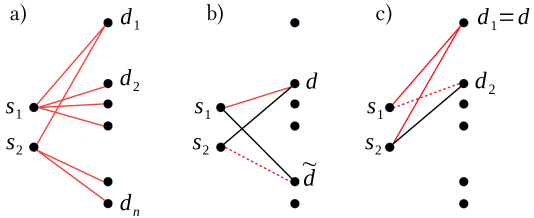
Figure 7: Illustration of the choice of entering variable in dashed lines when $D_{1}$ and $D_{2}$ non empty. Edges belonging to the optimum tree a) are in red.

Otherwise, without loss of generality we can assume $D_{2}$ empty and $D_{1}=\{2,\ldots,n\}$ (see Figure 8). $s_{2}$ is a leaf adjacent to $d_{1}$ in $x^{*}$ so the demand at $d_{1}$ is greater to the supply at $s_{2}$. Then, in an admissible tree, $d_{1}$ cannot be a leaf adjacent to $s_{2}$. Since $d\neq d_{1}$, $d_{1}$ is a leaf and it has to be adjacent to $s_{1}$ in $x$. We make the variable $(s_{2},d_{1})$ enter the basis. The corresponding cycle is $s_{2}ds_{1}d_{1}$ and $(s_{1},d)$ and $(s_{2},d)$ are present edges in the optimum $x^{*}$. By Lemma 4.1 this pivot is increasing. Denote by $x^{2}$ the new spanning tree. The potential leaving variables are only $(s_{1},d_{1})$ and $(s_{2},d)$ but it cannot be $(s_{1},d_{1})$ otherwise $d_{1}$ would be a leaf adjacent to $s_{2}$ in $x^{2}$. Therefore, $(s_{2},d)$ has been deleted and $d$ is now a leaf adjacent to the correct supply node in $x^{2}$ so we can delete the demand leaf $d$.

In $x^{2}$, $d_{1}$ is now adjacent to both supply nodes and all other demand nodes are adjacent to $s_{2}$. We enter the variable $(s_{1},d_{2})$ into the basis. The corresponding cycle $s_{1}d_{1}s_{2}d_{2}$ is improving since $(s_{1},d_{2})$ and $(s_{2},d_{1})$ are in $x^{*}$. Similarly to above, $(s_{1},d_{1})$ cannot be the leaving variable otherwise $d_{1}$ would become a leaf adjacent to $s_{2}$. Therefore, in the new spanning tree $x^{2}$, $d_{2}$ is a leaf adjacent to the correct supply node so we can delete it.

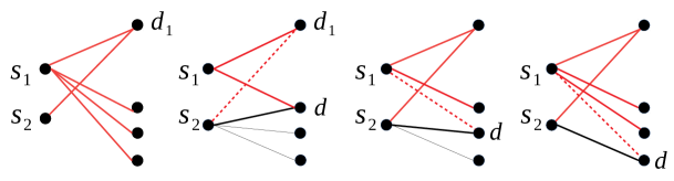
Figure 8: Illustration of the choice of entering variable in dashed lines when $D_{2}$ null. Edges belonging to the optimum tree on the left are in red.

Note that in all pivot steps considered here we delete a demand node. In the new spanning tree, either $d_{1}$ is a leaf or $D_{1}$ or $D_{2}$ are null which are the cases we handled. The induction therefore holds and we can get to $n^{\prime}=1$ in at most $n-1$ steps. For $n^{\prime}=1$ there is only one spanning tree which is the optimum.

Case 2: $d=d_{1}$
We have already considered the case where $D_{1}$ or $D_{2}$ are empty so now assume this is not the case. Therefore $d_{2}\in D_{1}$ and $d_{2}$ is a leaf adjacent to $s_{2}$ in $x$ (see Figure 7c).

We make the edge $(s_{1},d_{2})$ enter the basis. The corresponding cycle is $s_{1}d_{1}s_{2}d_{2}$. This is an improving cycle according to Lemma 4.1 given that edges $(s_{1},d_{2})$ and $(s_{2},d_{1})$ are present in $x^{*}$. Denote by $x^{2}$ the new vertex of the polytope. Either edge $(s_{1},d_{1})$ or $(s_{2},d_{2})$ has been removed. If $(s_{2},d_{2})$ was removed, $d_{2}$ is a leaf in $x^{2}$ adjacent to $s$ in $x^{2}$, likewise in $x^{*}$. Removing node $d_{2}$ therefore gives the result by induction. Otherwise, $(s_{1},d_{1})$ has been removed so in $x^{2}$, the demand node adjacent to both supply nodes is now $d_{2}\neq d_{1}$ and we use case 1.

We proved that the monotone diameter is $\leq n$. The bound $n$ can be attained potentially if there exists at least one vertex with $d=d_{1}$ and $D_{1},D_{2}$ non empty. This can only happen if $n\geq 3$, otherwise the monotone diameter is $n-1$. ∎

Conjecture 4.2.

The monotone diameter of $m\times n$ transportation polytopes is linear in $m$ and $n$.

Acknowledgements: The authors are grateful to Amitabh Basu, Laurent Poirrier, Francisco Santos, Laura Sanità, Sean Kafer and Xiaotie Chen for several remarks and comments that were useful to the creation of this manuscript. The first and second author were partially supported by NSF grant DMS-1818969. The first author was also supported by École Polytechnique.

References

- [1] Ilan Adler, Christos Papadimitriou, and Aviad Rubinstein. On simplex pivoting rules and complexity theory. In Integer Programming and Combinatorial Optimization 2014, IPCO’14, pages 13–24. Springer International Publishing, Cham, 2014.
- [2] Roger E. Behrend. Fractional perfect b-matching polytopes I: General theory. Linear Algebra and its Applications, 439(12):3822–3858, 2013.
- [3] Nicolas Bonifas, Marco Di Summa, Friedrich Eisenbrand, Nicolai Hähnle, and Martin Niemeier. On sub-determinants and the diameter of polyhedra. Discrete & Computational Geometry, 52(1):102–115, 2014.
- [4] Steffen Borgwardt, Jesús A. De Loera, and Elisabeth Finhold. The diameters of network-flow polytopes satisfy the Hirsch conjecture. Mathematical Programming, 171(1-2):283–309, 2018.
- [5] Jesús A. De Loera. New insights into the complexity and geometry of linear optimization. Optima, 87:1–11, 2011.
- [6] Jesús A. De Loera, Sean Kafer, and Laura Sanità. Pivot rules for circuit-augmentation algorithms in linear optimization. 2019. preprint available at arXiv:1909.12863.
- [7] Jesús A. De Loera, Hemmecke Raymond, and Köppe Matthias. Algebraic and geometric ideas in the theory of discrete optimization, volume 14 of MOS-SIAM Series on Optimization. Society for Industrial and Applied Mathematics (SIAM), Philadelphia, 2013.
- [8] Alberto Del Pia and Carla Michini. Short simplex paths in lattice polytopes. arXiv e-prints, page arXiv:1912.05712v1, 2019.
- [9] Mike Develin. LP-orientations of cubes and crosspolytopes. Advances in Geometry, 4(4):459–468, 2004.
- [10] Jack Edmonds. Maximum matching and a polyhedron with 0,1-vertices. Journal of Research of the National Bureau of Standards, 69B(1-2):125–130, 1965.
- [11] John Fearnley and Rahul Savani. The complexity of the simplex method. In Symposium on Theory of Computing 2015, STOC’15, pages 201–208. ACM, New York, 2015.
- [12] Mackenzie J. Gallagher and Jr Walter D. Morris. A proof of the strict monotone 5-step conjecture. arXiv e-prints, page arXiv:1806.03403, 2018.
- [13] Peter Gritzmann and Bernd Sturmfels. Minkowski addition of polytopes: computation complexity and applications to Gröbner bases. SIAM Journal on Discrete Mathematics, 6(2):246–269, 1993.
- [14] Gil Kalai. Upper bounds for the diameter and height of graphs of convex polyhedra. Discrete Comput. Geom., 8(4):363–372, 1992.
- [15] Tomonari Kitahara, Tomomi Matsui, and Shinji Mizuno. On the number of solutions generated by Dantzig’s simplex method for LP with bounded variables. Pacific journal of optimization, 8(3):447–455, 2012.
- [16] Tomonari Kitahara and Shinji Mizuno. A bound for the number of different basic solutions generated by the simplex method. Mathematical Programming, 137(1):579–586, 2013.
- [17] Victor Klee. A class of linear programming problems requiring a large number of iterations. Numerische Mathematik, 7(4):313–321, Aug 1965.
- [18] Victor Klee. Heights of convex polytopes. Journal of Mathematical Analysis and Applications, 11:176 – 190, 1965.
- [19] Victor Klee and George J. Minty. How good is the simplex algorithm? In Inequalities–III, Proceedings Third Symposium, 1969, pages 159–175. Academic Press, New York, 1972.
- [20] Takahito Kuno, Yoshio Sano, and Takahiro Tsuruda. Computing Kitahara–Mizuno’s bound on the number of basic feasible solutions generated with the simplex algorithm. Optimization Letters, 12(5):933–943, 2018.
- [21] Jed Mihalisin and Victor Klee. Convex and linear orientations of polytopal graphs. Discrete & Computational Geometry, 24(2):421–436, 2000.
- [22] Shmuel Onn and Rom Pinchasi. A note on the minimum number of edge-directions of a convex polytope. Journal on Combinatorial Theory, Series A, 107(1):147–151, 2004.
- [23] James B. Orlin. A polynomial time primal network simplex algorithm for minimum cost flows. Mathematical Programming, 77:109–129, 1997.
- [24] Igor Pak. Four questions on Birkhoff polytope. Annals of Combinatorics, 4(1):83–90, 2000.
- [25] Julian Pfeifle and Günter M. Ziegler. On the monotone upper bound problem. Experimental Mathematics, 13(1):1–11, 2004.
- [26] Fred J. Rispoli. The monotonic diameter of the perfect matching and shortest path polytopes. Operations Research Letters, 12(1):23–27, 1992.
- [27] Fred J. Rispoli. The monotonic diameter of the perfect 2-matching polytope. SIAM Journal on Optimization, 4(3):455–460, 1994.
- [28] Fred J. Rispoli. The monotonic diameter of traveling salesman polytopes. Operations Research Letters, 22(2-3):69–73, 1998.
- [29] Fred J. Rispoli and Steven Cosares. A bound of 4 for the diameter of the symmetric traveling salesman polytope. SIAM Journal on Discrete Mathematics, 11(3):373–380, 1998.
- [30] Francisco Santos. Recent progress on the combinatorial diameter of polyhedra and simplicial complexes. In Symposium on Computational Geometry 2013, SoCG’13, pages 165–166, 2013.
- [31] Masaya Tano, Ryuhei Miyashiro, and Tomonari Kitahara. A generalization of the steepest-edge rule and its number of simplex iterations for a nondegenerate LP. arXiv e-prints, page arXiv:1803.05167v1, 2018.
- [32] Michael J. Todd. The monotonic bounded Hirsch conjecture is false for dimension at least 4. Mathematics of Operations Research, 5(4):599–601, 1980.
- [33] Michael J. Todd. The many facets of linear programming. Mathematical Programming Series B, 91(3):417–436, 2002.
- [34] Donald M. Topkis. Adjacency on polymatroids. Mathematical Programming, 30(2):229–237, 1984.
- [35] Norman Zadeh. A bad network problem for the simplex method and other minimum cost flow algorithms. Mathematical Programming, 5(1):255–266, 1973.