The effect of CO$-$H₂O collisions in the rotational excitation of cometary CO

Abstract

We present the first accurate rate coefficients for the rotational excitation of CO by H₂O in the kinetic temperature range 5-100 K. The statistical adiabatic channel method (SACM) is combined with a high-level rigid-rotor CO$-$H₂O intermolecular potential energy surface. Transitions among the first 11 rotational levels of CO and the first 8 rotational levels of both para-H₂O and ortho-H₂O are considered. Our rate coefficients are compared to previous data from the literature and they are also incorporated in a simple non-LTE model of cometary coma including collision-induced transitions, solar radiative pumping and radiative decay. We find that the uncertainties in the collision data have significant influence on the CO population distribution for H₂O densities in the range $10^{3}-10^{8}$ cm^-3. We also show that the rotational distribution of H₂O plays an important role in CO excitation (owing to correlated energy transfer in both CO and H₂O), while the impact of the ortho-to-para ratio of H₂O is found to be negligible.

1 Introduction

Rate coefficients (or cross sections) for molecular collisional excitation are needed to model both thermal balance and spectral line formation in astrophysical objects such as interstellar clouds, protoplanetary disks and planetary/cometary atmospheres. In such environments, the density can be so low ($n\ll 10^{10}$ cm^-3) that collisions indeed cannot maintain a local thermodynamical equilibrium (LTE) everywhere. Until recently, the accuracy of theoretical collision data was mainly inferred indirectly by comparison with related processes such as line broadening cross sections (see e.g Mengel, Flatin & De Lucia, 2000; Wiesenfeld & Faure, 2010). In the last decade, there has been huge progress in measuring state-to-state collision cross sections at very low energy ($E_{col}\sim$1 meV) (see Naulin & Bergeat, 2018, for a recent review). Detailed comparisons between quantum calculations and merged-beam measurements have thus allowed experimentalists to verify theoretical cross sections in the ’cold’ regime (equivalent temperature $\sim$ 10 K) where quantum effects such as resonances are predominant. Theory has passed all experimental tests so far, establishing the reliability of modern collisional data used in astrophysical models (Chefdeville et al., 2013, 2015; Gao et al., 2019; Bergeat et al., 2019). These theoretical values have been obtained for ’simple’ collision systems such as rigid rotors excited by light atomic or diatomic perturbers, in particular He atoms and H₂ molecules which are the most abundant collisional partners in the interstellar medium (ISM).

However, collision rate coefficients are also needed for systems involving heavy and even polyatomic perturbers, which challenge current computational capabilities. For instance, in the thermosphere of Titan, N₂ and CH₄ are the most abundant collisional perturbers (Rezac et al., 2013). In cometary comas, collisional excitation is generally dominated by H₂O (and/or electrons) and, for comets at large heliocentric distances, by CO (Bockelée-Morvan et al., 2004). The main difficulty with such systems is the excessively large number of angular couplings between the target and the projectile which make full quantum calculations prohibitively expensive, both in terms of computer time and memory requirements. As a result, to the best of our knowledge, the only sets of rotationally-resolved rate coefficients for the water perturber are those of Green (1993) for CO$-$H₂O, those of Buffa et al. (2000) for H₂O$-$H₂O and those of Dubernet & Quintas-Sánchez (2019) for HCN$-$H₂O. The two former sets were estimated using crude treatments while the latter was obtained using only partially converged coupled-states (CS) calculations.

In this paper, we present the first quantum calculations for the rotational excitation of CO by H₂O molecules. This is also the first study to consider the two nuclear-spin isomers of H₂O, ortho- and para-H₂O (hereafter referred as o-H₂O and p-H₂O), as two distinct perturbers. The statistical adiabatic channel model (SACM) is used as a validated alternative to prohibitive close-coupling calculations (Loreau, Lique & Faure, 2018a; Loreau, Faure & Lique, 2018b) and it is combined here with the recent ab initio CO$-$H₂O interaction potential computed by Kalugina et al. (2018). The CO$-$H₂O collision system is of great importance in comets but also in protoplanetary and debris disks when the gas originates from ices in planetesimals (Matrà et al., 2015). In addition to providing collision data for the first 11 rotational levels of CO, we also present a non-LTE model for the CO excitation in comets, including collision-induced transitions due to p-H₂O and o-H₂O, radiative pumping of the $v=0\to 1$ band due to solar photons and radiative decay due to spontaneous emission. A key objective is to assess the impact of accurate CO$-$H₂O collisional data on the rotational distribution of cometary CO. The next Section describes the CO$-$H₂O scattering calculations. Section 3 compares the present results with previous collisional data for CO. In Section 4, we present simple nonequilibrium calculations for the excitation of CO in comets. Concluding remarks are made in Section 5.

2 Quantum statistical calculations

The computation of inelastic cross sections from first principles consists of two main steps. First, the electronic Schrödinger equation is solved using quantum chemistry methods. Within the Born-Oppenheimer approximation, a single intermolecular potential energy surface (PES) governing the motion of the nuclei is defined as function of nuclear coordinates. The nuclear motion is solved separately, in a second step, using quantum or (semi)classical scattering methods. We describe in this section our calculations for the CO$-$H₂O system.

2.1 Potential energy surface

The CO$-$H₂O scattering calculations presented below are based on the high-level ab initio intermolecular potential recently determined by Kalugina et al. (2018). The interacting molecules CO and H₂O are considered as rigid-rotors, with geometries corresponding to their ground vibrational state. The PES was calculated at 93,000 relative orientations using the explicitly-correlated single- and double-excitation coupled cluster theory with a non-iterative perturbative treatment of triple excitations [CCSD(T)-F12a] along with the augmented correlation-consistent aug-cc-pVTZ basis sets (AVTZ hereafter). The intermolecular energies were then fitted to a body-fixed expansion expressed as a sum of spherical harmonic products and a Monte-Carlo estimator was employed to select the largest expansion terms. This CO$-$H₂O PES has a global well depth $D_{e}=646.1$ cm^-1 for an intermolecular center-of-mass separation $R=7.42$ $a_{0}$ and a planar configuration OC$-$H₂O, with a weak hydrogen bond between the C atom of CO and one H atom of H₂O. Bound-state rovibrational energy calculations using this PES have been found in very good agreement with experiments (Barclay et al., 2019), confirming the good accuracy of the potential. We note that a full-dimensional CO$-$H₂O PES was recently computed at the same level (CCSD(T)-F12a/AVTZ) by Liu & Li (2019). These authors found a similar but deeper well depth ($D_{e}=685.5$ cm^-1), which is due to the basis set superposition error (BSSE) not corrected by Liu & Li (2019).

2.2 The statistical adiabatic channel model

Rigorous close-coupling quantum scattering calculations become impracticable when the number of coupled channels exceed typically 10,000. In such situation, statistical methods may provide a useful alternative. Statistical theories generally apply when a collisional system can access a deep well on the PES and the lifetime of the complex is sufficiently long. We have recently (Loreau, Lique & Faure, 2018a) developed a statistical approach inspired by the statistical adiabatic channel model (SACM) of Quack & Troe (1975). In our implementation, we diagonalize the Hamiltonian excluding the kinetic term in the basis of rotational functions for the collision. In the present case, the angular functions are products of Wigner rotation matrices for H₂O and spherical harmonics for CO as well as for the relative orbital motion (Phillips, Maluendes & Green, 1995). This expansion corresponds to the coupling of the angular momenta ${\boldsymbol{j}_{1}}$ of H₂O, ${\boldsymbol{j}_{2}}$ of CO, and ${\boldsymbol{\ell}}$ for the relative motion to form the total angular momentum $\boldsymbol{J=j_{1}+j_{2}+\ell}$. Upon diagonalization, for each value of $J$ we obtain a set of adiabatic rotational curves as a function of the intermolecular distance $R$ with an asymptotic value given by the sum of rotational energies of H₂O and CO. These curves possess centrifugal barriers that depend on the orbital quantum number $\ell$, and for a given initial state, the collision is assumed to take place if the collision energy is larger than the height of the barrier. The probability is then divided equally among the channels for which the energy is larger than their respective centrifugal barriers, allowing us to compute state-to-state cross sections and rate coefficients.

This procedure was found to provide rate coefficients with an average accuracy better than 50% for ion-molecule systems up to room temperature (Loreau, Lique & Faure, 2018a). In the case of CO$-$H₂O, the SACM partial rate coefficients (computed for a total angular momentum $J=0$) were shown to be accurate to within 40% up to 100 K (Loreau, Faure & Lique, 2018b). Full comparisons between SACM and close-coupling calculations can be found in the two papers by Loreau and co-workers.

In this paper the cross sections were calculated for transitions among the first 11 energy levels of CO (up to $j_{2}=10$) and the first 8 energy levels of both p-H₂O and o-H₂O (up to $j_{1}=3$) and for collision energies between 0 and 500 cm^-1 in order to derive rate coefficients up to $T=100$ K. This requires to obtain all the adiabatic curves up to a total energy of 750 cm^-1. The basis set of angular functions included levels up to $j_{1}=5$ and $j_{2}=15$, and tests were performed to ensure the convergence of the adiabatic curves with respect to the size of the basis set. The rotational constant of CO was taken to be $B_{0}=1.92253$ cm^-1, while the energy of the rotational levels of H₂O, $E_{j_{1}k_{a}k_{c}}$, was obtained using the effective Hamiltonian of Kyrö (1981). They are labeled with $j_{1}$, $k_{a}$, and $k_{c}$, where $k_{a}$ and $k_{c}$ are pseudoquantum numbers corresponding to the projection of the angular momentum $j_{1}$ along the axis of least and greatest moment of inertia, respectively. Adiabatic curves were generated for values of the total angular momentum from $J=0$ up to $J=100$ for o-H₂O and p-H₂O separately. High total angular momentum values were found to be necessary as the cross section converges very slowly with $J$ due to the deep well in the PES as well as to the large reduced mass of H₂O-CO.

Two sets of rate coefficients describing the excitation of CO by H₂O were considered: the first consists of rate coefficients for which H₂O is in the ground rotational state of its nuclear-spin isomer, i.e. $k_{j_{2}\rightarrow j_{2}^{\prime}}(T)=k_{0_{00},j_{2}\rightarrow 0_{00},j_{2}^{\prime}}(T)$ or $k_{1_{01},j_{2}\rightarrow 1_{01},j_{2}^{\prime}}(T)$ for p-H₂O and o-H₂O, respectively. This set of “ground-state” rate coefficients neglects the simultaneous excitation of CO and H₂O as well as the fact that excited rotational states of H₂O can be significantly populated. Such an approximation is therefore expected to be accurate only at very low temperatures.

To take into account the transitions in H₂O, we constructed a second set of rate coefficients (separately for p-H₂O and o-H₂O) by summing over all possible final states of H₂O, and averaging over the initial rotational states of H₂O assuming a thermal population distribution:

$$k_{j_{2}\rightarrow j_{2}^{\prime}}(T)=\sum_{j_{1}k_{a}k_{c}j_{1}^{\prime}k_{a}^{\prime}k_{c}^{\prime}}P_{j_{1}k_{a}k_{c}}(T)k_{j_{1}k_{a}k_{c},j_{2}\rightarrow j_{1}^{\prime}k_{a}^{\prime}k_{c}^{\prime},j_{2}^{\prime}}(T),$$ (1)

where

$$P_{j_{1}k_{a}k_{c}}(T)=\frac{g_{j_{1}}\exp(-E_{j_{1}k_{a}k_{c}}/k_{B}T)}{\sum_{j_{1}k_{a}k_{c}}g_{j_{1}}\exp(-E_{j_{1}k_{a}k_{c}}/k_{B}T)}$$ (2)

is the Boltzmann population of level $j_{1}k_{a}k_{c}$ at temperature $T$ and $k_{B}$ is the Boltzmann constant. This set of “thermalized” rate coefficients assumes that the kinetic and rotational temperatures are equal, and satisfies detailed balance. These thermalized rate coefficients can be much larger than the ground-states values, even at low temperature, owing to correlated rotational energy transfer in both collision partners (see below). All de-excitation rate coefficients are available as supplementary material. Excitation rate coefficients can be derived using the detailed balance principle.

3 Results

Rate coefficients for the rotational excitation of CO by H₂O are presented below at three kinetic temperatures, 10, 50 and 100 K, for transitions out of the ground rotational state of CO ($j_{2}$=0) as functions of the final $j_{2}$ ($j^{\prime}_{2}=1-10$). In Fig. 1, four sets of data are presented, corresponding to the “ground-state” and “thermalized” SACM rate coefficients defined above with p-H₂O and o-H₂O as colliders. It is seen that all four sets have very similar rate coefficients at 10 K and that the transition $j_{2}=0\to 1$ dominates. Small differences between thermalized and ground-state rate coefficients were expected at 10 K because i) only the ground-state of p-H₂O and o-H₂O is significantly populated at thermal equilibrium and ii) the excitation of H₂O is inhibited because the rotational thresholds are larger than 10 K (23 K and 54 K for the first excitation in o-H₂O and p-H₂O, respectively). In fact, however, substantial differences (more than a factor of 2) are found for transitions with $j^{\prime}_{2}>3$ whose rate coefficients are smaller than $10^{-11}$ cm³s^-1. For instance, the thermalized and ground-state rate coefficients for the excitation $j_{2}=0\to 4$ ($\Delta E$=38.4 cm^-1) by p-H₂O are $1.26\times 10^{-12}$ cm³s^-1 and $3.16\times 10^{-13}$ cm³s^-1, respectively. The much larger thermalized value is due to the correlation between the CO excitation $j_{2}=0\to 4$ ($\Delta E$=38.4 cm^-1) and the simultaneous H₂O de-excitation $j_{1}k_{a}k_{c}=1_{11}\to 0_{00}$ ($\Delta E$=37.1 cm^-1). This particular process provides a major contribution to the thermalized rate coefficient, despite the low population of the $1_{11}$ level at 10 K ($\sim$1%). We also note that the near-resonant character of this correlated (de)excitation is not accounted for by SACM calculations and that close-coupling calculations would predict an even larger thermalized rate coefficient. At 50 and 100 K, the differences between the thermalized and the ground-state rate coefficients are clearly visible, reflecting both the larger population of excited H₂O levels (thus pair correlations) and the opening of excitation channels in H₂O. In particular, the transitions $j_{2}=0\to 2,3$ are preferred in the thermalized data at 100 K while $j_{2}=0\to 1$ is favored in the ground-state data. We also note that the difference between p-H₂O and o-H₂O is very small, both for thermalized and ground-state data, suggesting that the ortho-to-para ratio (OPR) of H₂O should not play a major role in the excitation of CO (see Section 4 below).

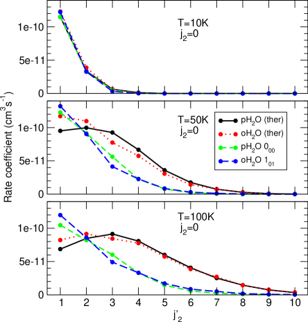
Figure 1: SACM rate coefficients for the rotational excitation of CO by H₂O from the ground state ($j_{2}$=0) to the lowest ten excited states. The projectiles p-H₂O and o-H₂O are assumed to be either thermalized at the kinetic temperature (10, 50 or 100 K) or in their ground rotational states $0_{00}$ and $1_{01}$, respectively. See text for details.

In Fig. 2, the above set of thermalized rate coefficients is compared to previous data from the literature: those of Biver et al. (1999) (denoted as B99) and those of Green (1993) (denoted as G93). Biver et al. (1999) assumed a total cross-section of $\sigma_{c}=2\times 10^{-14}$ cm^-2, with no energy dependence. This value was derived from room temperature pressure broadening measurements on H₂O-H₂O (Biver, 1997), with an estimated uncertainty of a factor of $\sim 2$. The total collisional rate coefficient was computed as $k_{c}(T)=\sigma_{c}\langle v(T)\rangle$, where $T$ is the kinetic temperature and $\langle v(T)\rangle$ is the thermal mean velocity of the CO molecule relative to the cometary gas. State-to-state rate coefficients from an initial CO level $j_{2}$ to a final level $j^{\prime}_{2}$ were then obtained as $k_{j_{2}\to j^{\prime}_{2}}(T)=k_{c}P_{j^{\prime}_{2}}(T)$, where $P_{j^{\prime}_{2}}(T)$ is the Boltzmann population of the final level $j^{\prime}_{2}$ at temperature $T$. This recipe corresponds to assuming that each collision redistributes the molecule according to the Boltzmann distribution, which has no physical basis, except that it satisfies the detailed balance principle (by construction). Green (1993), on his side, combined line shape measurements on N₂-H₂O with a rate-law derived from the infinite-order-sudden (IOS) approximation. The total excitation rates were expected to be rather accurate (about 10%) at room temperature, where the rate-law parameters were fitted. It should be noted that in contrast to our SACM calculations, the B99 and G93 collision data sets do not distinguish between p-H₂O and o-H₂O. It is found in Fig. 2 that the magnitude and the $\Delta j_{2}=j^{\prime}_{2}-j_{2}$ dependence of the rate coefficients are reasonably described by the B99 and G93 data sets: the largest rate coefficients are $\sim 10^{-10}$ cm³s^-1 and they (globally) slowly decrease with increasing $\Delta j_{2}$. The overall agreement is somewhat surprising, in particular for the B99 data set given the simplicity of the prescription. We note, however, that differences larger than a factor of 2 are observed for transitions with $\Delta j_{2}>2$ and, more generally, that the B99 set overestimates while the G93 set tends to underestimate the SACM rate coefficients.

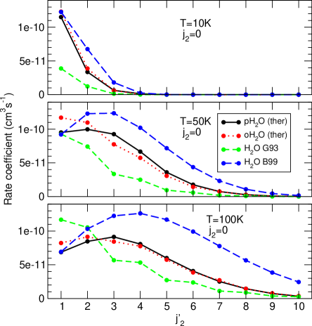
Figure 2: Same as Fig. 1. The thermalized SACM data for p-H₂O and o-H₂O are compared to the data of Biver et al. (1999) and Green (1993). See text for details.

It is now interesting to compare the efficiency of H₂O relative to other colliders for exciting CO. In Fig. 3, the thermalized SACM rate coefficients for CO$-$H₂O are compared to the corresponding data for CO$-$H (Yang et al., 2013), CO$-$He (Cecchi-Pestellini et al., 2002), CO$-$p-H₂ and CO$-$o-H₂ (Yang et al., 2010). These latter four sets of data were obtained from quantum close-coupling calculations combined with modern PES. Their accuracy at the state-to-state level is expected to be very good (about 20%), as verified experimentally for CO$-$He and CO$-$H₂ (Carty et al., 2004; Chefdeville et al., 2015). We can first observe that, at 10 K, p-H₂O and o-H₂O are the most effective colliders with a rate coefficient for the transition $j_{2}=0\to 1$ that is a factor of $\sim 2$ larger than those for the other colliders. Atomic hydrogen is the less effective, with rate coefficients lower than $10^{-11}$ cm³s^-1. At larger temperatures, the $\Delta j_{2}$ dependence of the rate coefficients is found to be very different for H₂O than for H and H₂: while the water rate coefficients slowly decrease with increasing $\Delta j_{2}$, a strong propensity rule with $\Delta j_{2}=2$ is observed for atomic and molecular hydrogen. As a result, the largest rate coefficients at 100 K are those of H and H₂ for the transition $j_{2}=0\to 2$. For transitions with $\Delta j_{2}>2$, however, H₂O is seen to be more than twice as effective as the other colliders. The magnitude of the rate coefficients for the excitation of CO by H₂O is thus rather similar to that of other neutral colliders. The main difference is the lack of strong propensity rules and the relatively slow decrease of the rate coefficients with increasing $\Delta j_{2}$. This reflects mainly the larger potential well depth but also the fact that SACM calculations are not able to catch resonance and interference effects (Loreau et al. 2018a, 2018b). In particular, as discussed above, SACM calculations are expected to underestimate near-resonant rotational energy transfers.

We note, finally, that free electrons provide another source of CO rotational excitation in astronomical environments. Owing to the small dipole of CO (0.11 D), however, rate coefficients for electron-impact rotational excitation do no exceed $\sim 2\times 10^{-8}$ cm³s^-1. This means that electrons compete with neutrals in exciting CO only when the electron-to-neutral number density ratio is larger than $\sim 10^{-2}$.

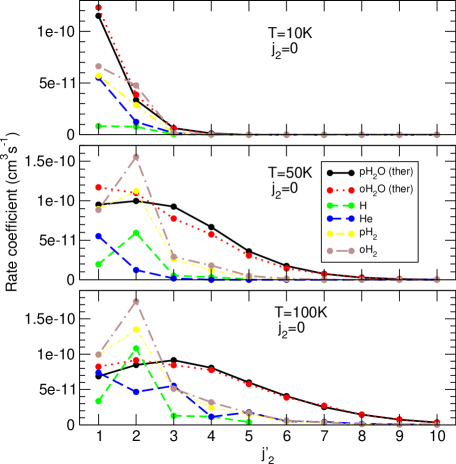
Figure 3: Same as Fig. 1. The thermalized SACM data for p-H₂O and o-H₂O are compared to the data for other projectiles: H, He, p-H₂ and o-H₂.

4 Non-LTE model of CO in comets

In this Section, we present a simple non-LTE model of CO excitation in a cometary coma. Our main objective is to assess the impact of the collisional rate coefficients on the predicted rotational populations of CO. We have chosen physical conditions corresponding to an average comet located at $R_{\rm h}$=1 AU from the Sun with a total production rate from the nucleus $Q_{\rm H_{2}O}=1\times 10^{29}$ s^-1, an expansion velocity $v_{\rm exp}=0.8$ km s^-1 and a neutral gas temperature $T_{k}$ in the range $10-100$ K. Water is assumed to be the dominant neutral collider in the coma. The H₂O density can be described by a standard isotropic Haser model (Haser, 1957):

$$n_{\rm H_{2}O}(r)=\frac{Q_{\rm H_{2}O}}{4\pi r^{2}v_{\rm exp}}\exp\left(-r\frac{\beta_{\rm H_{2}O}}{v_{\rm exp}}\right),$$ (3)

where $r$ is is the nucleocentric distance and $\beta_{\rm H_{2}O}$ is the H₂O photodissociation rate at $R_{\rm h}$=1 AU. The coupled radiative transfer and statistical equilibrium (SE) equations are solved with the public version of the RADEX code using the large velocity gradient (LVG) approximation. The problem is treated as both local and steady-state by running a grid of RADEX calculations covering a range of H₂O densities. We thus assume that the physical processes driving the population are much faster than variations in physical conditions of the coma. Note that we also neglect CO photodissociation (the CO lifetime is about $5.3\times 10^{5}$ s at $R_{\rm h}$=1 AU for the active Sun (Huebner, Keady & Lyon, 1992)) so that chemical processes (formation and destruction of CO) are omitted from the SE equations. This approach may not be valid over the whole coma and more elaborate and accurate non-LTE treatments exist in the literature (Zakharov et al., 2007; Yamada et al., 2018). We believe, however, that the main features of the collisional effects are well captured by our simple model.

The input parameters to RADEX are the kinetic temperature, $T_{k}$, the column density of CO, $N$(CO), the line width, $\Delta v$, and the density of the collider, here $n_{\rm H_{2}O}$. Three kinetic temperatures were selected: 10, 50 and 100 K. The column density was fixed at $N({\rm CO})=10^{14}$ cm^-2, which is the typical magnitude at $r\sim 1000$ km for a CO/H₂O abundance ratio of $\sim 10$% (e.g. Lupu et al., 2007). We have checked, however, that the relative populations are not sensitive to the column density provided that $N({\rm CO})<10^{16}$ cm^-2 (i.e. the lines are optically thin). The water density is varied in the large range $10^{-3}-10^{13}$ cm^-3 corresponding to nucleocentric distances between 1 and $10^{6}$ km in the Haser model, as plotted in Fig. 4. The line width is fixed at 1.6 km s^-1, i.e. $\Delta v=2\times v_{\rm exp}$. Finally, the background radiation field includes both the 2.73 K cosmic microwave background (CMB) and the Sun radiation. This latter contribution is taken as a diluted blackbody of 5770 K with the dilution factor $W=\Omega_{S}/4\pi$, where $\Omega_{S}\sim 6.79\times 10^{-5}$ sr is the Sun solid angle seen at $R_{\rm h}$=1 AU.

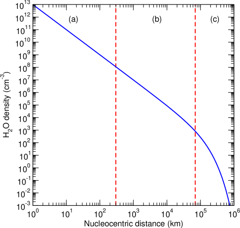
Figure 4: Coma density profile of H₂O in the Haser’s model. The photodissociation rate was taken as $\beta_{\rm H_{2}O}=1.042\times 10^{-5}$ s^-1 from Zakharov et al. (2007). The dashed lines delineate, for a production rate $Q_{\rm H_{2}O}=1\times 10^{29}$ s^-1, the three approximate density regimes: (a) LTE equilibrium, (b) non-LTE regime, and (c) fluorescence equilibrium. See text for details.

Input data include the CO energy levels $(v_{2},j_{2})$ ($v_{2}$ is the CO vibrational quantum number), the spontaneous emission Einstein coefficients and the collisional rate coefficients. Level energies and Einstein coefficients were taken from the HITRAN database (Gordon et al., 2017). Only the first excited vibrational level $v_{2}=1$ was taken into account because the solar excitation rate of $v_{2}=1$ is at least two orders of magnitude greater than those of $v_{2}>1$ (Crovisier & Le Bourlot, 1983). Our model thus include the lowest 80 ro-vibrational levels of CO, i.e. up to level $(v_{2},j_{2})=(1,32)$ which lies 4148 cm^-1 above the ground-state $(0,0)$. Since our SACM rate coefficients are available for the lowest 11 rotational levels only, we had to extrapolate the collisional data above $j_{2}=10$. It should be noted, however, that the corresponding levels are negligibly populated (less than 1%) at the investigated temperatures and the extrapolated collisional data play only a minor role in the SE equations. In practice, the total de-excitation rotational rate coefficients were simply fixed at $10^{-10}$ cm³s^-1 with an equal distribution among final levels and no temperature dependence. Similarly the total de-excitation vibrational rate coefficients were fixed at $10^{-13}$ cm³s^-1 (with again an equal distribution among final levels), as suggested by the CO($v_{2}=1$)$-$H₂O quenching measurements of Wang, Gu & Kong (1999) performed at 300 K. Finally, for pure rotational transitions involving rotational levels $j_{2}\leq 10$ within $v_{2}=1$, we adopted the corresponding rate coefficients within $v_{2}=0$. Rotational rate coefficients indeed depend only weakly on the vibrational state (Carty et al., 2004). This extrapolation procedure was used for the SACM, the B99 and the G93 collision data sets.

The population distribution of the CO rotational levels $j_{2}$ in $v_{2}=0$ is thus governed by the balance between the collision-induced transitions, the vibrational excitation ($v_{2}=0\to 1$) by the solar infrared radiation field, the rotational excitation by the CMB radiation field and the radiative decay due to spontaneous emission. The results of our non-LTE model are presented in Fig. 5 where the population of levels $j_{2}$ is plotted as function of the H₂O density for the selected kinetic temperatures 10, 50 and 100 K. The set of thermalized SACM rate coefficient is employed here with an OPR for H₂O equal to 3. We can clearly observed the presence of three different regimes: the fluorescence equilibrium at low densities ($n_{\rm H_{2}O}\lesssim 10^{3}$ cm^-3), the non-LTE regime in the range $10^{3}\lesssim n_{\rm H_{2}O}\lesssim 10^{8}$ cm^-3 and the LTE-regime at larger densities. Thus, for a production rate $Q_{\rm H_{2}O}=1\times 10^{29}$ s^-1, LTE applies at $r\lesssim 300$ km, i.e. in the inner coma, while the fluorescence equilibrium distribution is completely established at $r\gtrsim 7\times 10^{4}$ km (see Fig. 4). The non-LTE regime extends typically from 300 to 70,000 km, representing about 10% of all CO molecules in the coma. We can notice in Fig. 5 that the non-LTE regime of densities does not significantly vary with temperature. In contrast, the LTE population distribution is very sensitive to the temperature: at 10 K significant populations ($>$1%) are found only for $j_{2}=0-3$ while at 100 K all levels $j_{2}=0-10$ are occupied above 2%.

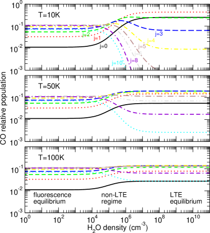
Figure 5: Level populations of CO ($j=0-6,8,10$) as functions of H₂O density for kinetic temperatures of 10, 50 and 100 K. The thermalized SACM rate coefficients are employed with an OPR of H₂O fixed at 3.

In the following, the H₂O density is fixed at $n_{\rm H_{2}O}=1.9\times 10^{5}$ cm^-3, which is representative of the non-LTE regime. The corresponding nucleocentric distance is $r\sim 7000$ km. In Fig. 6 the CO relative population is plotted as function of $j_{2}$ for the two sets of SACM rate coefficients (thermalized and ground-state) and for an OPR of H₂O equal to 1 and 3. The OPR of H₂O in comets is debated but values are generally comprised between 1 and 3, with a median equal to 2.9 (see Faure et al., 2019, and references therein). We first observe that the impact of the OPR of water is negligible, as expected from the small differences seen in Fig. 1. It can be also noticed that the thermalized SACM rate coefficients predict a more peaked distribution than the ground-state rate coefficients, with a greater population for low $j_{2}$ levels. The relative difference is found to reach $\sim 60$% at 10 K for $j_{2}=2$. This effect is due to pair correlations between CO and H₂O transitions, as discussed in Section 3. Perhaps surprisingly, the influence of the H₂O rotational distribution is found to be less important at higher temperature. In fact, this mainly reflects the LTE distributions which are closer to the fluorescence equilibrium distribution at 50 K and mostly 100 K than at 10 K, attenuating the impact of collisional data.

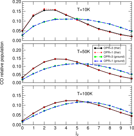
Figure 6: CO population distribution at a fixed H₂O density of $1.9\times 10^{5}$ cm^-3 for the three kinetic temperatures 10, 50 and 100 K. The SACM thermalized and ground-state rate coefficients are employed with an OPR of H₂O equal to 1 and 3. See text for details.

Finally, in Fig. 7 we compare the CO rotational populations as predicted by our thermalized SACM rate coefficients (with an OPR of H₂O fixed at 3) and by the B99 and G93 rate coefficients. As in Fig. 6, the influence of collisional data is found to decrease with temperature, which again reflects the relative deviation between the LTE and the fluorescence equilibrium distribution. At 10 K, the uncertainties in collisional data have the largest impact with relative differences up to a factor of $\sim 3$ for $j_{2}=1$. The B99 set overestimates while the G93 set underestimates the populations of levels $j_{2}\lesssim 4$, which is consistent with the trend in the rate coefficients shown in Fig. 2. For levels with $j_{2}>4$, however, the reverse is observed, emphasizing the role of collisional transitions out of $j_{2}>0$.

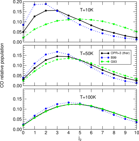
Figure 7: Same as Fig. 6. Three sets of collisional rate coefficients are employed: the thermalized SACM set with the OPR of H₂O fixed at 3, the B99 set and the G93 set. See text for details.

In summary, using a simple non-LTE model of CO in standard cometary conditions, we have found that uncertainties in the collisional rate coefficients have a significant impact on the CO population distribution in the non-LTE regime ($n_{\rm H_{2}O}\sim 10^{5}$ cm^-3). In particular, the CO rotational populations predicted by three different collisional data sets were found to differ by up to a factor of 3 at 10 K. Thanks to our SACM rate coefficients, we were also able to demonstrate that the H₂O rotational distribution plays an important role, even at low temperature (due to correlated rotational energy transfers) while the OPR of H₂O has an almost negligible influence.

5 Concluding remarks

We have provided the first quantum rate coefficients for the rotational excitation of CO by p-H₂O and o-H₂O. These rate coefficients were obtained by combining SACM calculations with a recent ab initio CO$-$H₂O PES computed at the CCSD(T)-F12a/AVTZ level. Rotational transitions among the first 11 energy levels of CO and the first 8 energy levels of both p-H₂O and o-H₂O were considered. Two different sets of rate coefficients were obtained: one corresponding to p-H₂O and o-H₂O in their ground rotational state and one corresponding to thermal distributions of each nuclear-spin isomer. Correlated energy transfer in both CO and H₂O was shown to be important while the differences between p-H₂O and o-H₂O were found to be small. Our set of “thermalized” rate coefficients was compared to previous data from the literature and significant differences were observed. We also found that H₂O is more effective than other colliders (H, He and H₂) for exciting CO transitions with $\Delta j_{2}>2$. Finally, we have assessed the impact of the collision data on the CO population distribution in a cometary coma using a simple non-LTE model including collision-induced transitions, radiative pumping and radiative decay. We have found that the uncertainties in the collision data can affect the rotational populations by large factors at low temperature and at H₂O densities $\sim 10^{3}-10^{8}$ cm^-3. In addition, the rotational distribution of H₂O was found to play a significant role so that a consistent non-LTE model of CO excitation should include a realistic (i.e. non-LTE) population distribution for H₂O. This in turn would require the knowledge of accurate H₂O-H₂O rotational rate coefficients, which are lacking in the literature. On the other hand, the OPR of H₂O was shown to have a negligible impact on the CO excitation, which removes one uncertainty from the interpretation of CO spectra.

Future studies will need to consider other linear targets such as CN, CS, HCO⁺ as well as non-linear species such as NH₃, H₂CO, etc. colliding with both H₂O and CO. The present SACM approach should be therefore extended to treat two non-linear polyatomic collision partners. We note that many data are available for the electron-impact rotational excitation of cometary molecules (e.g. Harrison, Faure & Tennyson, 2013). Comparing the efficiency of electrons relative to neutrals (H₂O and CO) will be very useful to distinguish between the different collisional non-LTE regimes in a comet (H₂O-, $e$- or CO-dominated). Finally, we strongly encourage modellers to use the present CO$-$H₂O data in any model of CO excitation in comets and, more generally, to use the ever-increasing amount of theoretical collision data available for astrophysical applications.

References

- Barclay et al. (2019) Barclay A. J., van der Avoird A., McKellar A. R. W., Moazzen-Ahmadi N., 2019, Physical Chemistry Chemical Physics (Incorporating Faraday Transactions), 21, 14911
- Bergeat et al. (2019) Bergeat A., Faure A., Morales S. B., Moudens A., Naulin C., 2019, J. Phys. Chem. A, in press
- Biver (1997) Biver N., 1997, PhD thesis, Université Paris VII
- Biver et al. (1999) Biver N. et al., 1999, AJ, 118, 1850
- Bockelée-Morvan et al. (2004) Bockelée-Morvan D., Crovisier J., Mumma M. J., Weaver H. A., 2004, The composition of cometary volatiles, Comets II, M. C. Festou, H. U. Keller, and H. A. Weaver (eds.), University of Arizona Press, Tucson, p.391-423
- Buffa et al. (2000) Buffa G., Tarrini O., Scappini F., Cecchi-Pestellini C., 2000, ApJS, 128, 597
- Carty et al. (2004) Carty D., Goddard A., Sims I. R., Smith I. W. M., 2004, J. Chem. Phys., 121, 4671
- Cecchi-Pestellini et al. (2002) Cecchi-Pestellini C., Bodo E., Balakrishnan N., Dalgarno A., 2002, ApJ, 571, 1015
- Chefdeville et al. (2013) Chefdeville S., Kalugina Y., van de Meerakker S. Y. T., Naulin C., Lique F., Costes M., 2013, Science, 341, 1094
- Chefdeville et al. (2015) Chefdeville S., Stoecklin T., Naulin C., Jankowski P., Szalewicz K., Faure A., Costes M., Bergeat A., 2015, ApJ, 799, L9
- Crovisier & Le Bourlot (1983) Crovisier J., Le Bourlot J., 1983, A&A, 123, 61
- Dubernet & Quintas-Sánchez (2019) Dubernet M. L., Quintas-Sánchez E., 2019, Molecular Astrophysics, 16, 100046
- Faure et al. (2019) Faure A., Hily-Blant P., Rist C., Pineau des Forêts G., Matthews A., Flower D. R., 2019, MNRAS, 487, 3392
- Gao et al. (2019) Gao Z., Loreau J., van der Avoird A., van de Meerakker S. Y. T., 2019, Physical Chemistry Chemical Physics (Incorporating Faraday Transactions), 21, 14033
- Gordon et al. (2017) Gordon I. E. et al., 2017, J. Quant. Spec. Radiat. Transf., 203, 3
- Green (1993) Green S., 1993, ApJ, 412, 436
- Harrison, Faure & Tennyson (2013) Harrison S., Faure A., Tennyson J., 2013, MNRAS, 435, 3541
- Haser (1957) Haser L., 1957, Bull. Soc. R. Sci. Liège, 43, 740
- Huebner, Keady & Lyon (1992) Huebner W. F., Keady J. J., Lyon S. P., 1992, Ap&SS, 195, 1
- Kalugina et al. (2018) Kalugina Y. N., Faure A., van der Avoird A., Walker K., Lique F., 2018, Phys. Chem. Chem. Phys., 20, 5469
- Kyrö (1981) Kyrö E., 1981, Journal of Molecular Spectroscopy, 88, 167
- Liu & Li (2019) Liu Y., Li J., 2019, Phys. Chem. Chem. Phys.,
- Loreau, Faure & Lique (2018b) Loreau J., Faure A., Lique F., 2018b, J. Chem. Phys., 148, 244308
- Loreau, Lique & Faure (2018a) Loreau J., Lique F., Faure A., 2018a, ApJ, 853, L5
- Lupu et al. (2007) Lupu R. E., Feldman P. D., Weaver H. A., Tozzi G.-P., 2007, ApJ, 670, 1473
- Matrà et al. (2015) Matrà L., Panić O., Wyatt M. C., Dent W. R. F., 2015, MNRAS, 447, 3936
- Mengel, Flatin & De Lucia (2000) Mengel M., Flatin D. C., De Lucia F. C., 2000, J. Chem. Phys., 112, 4069
- Naulin & Bergeat (2018) Naulin C., Bergeat A., 2018, Chapter 3: Low-energy Scattering in Crossed Molecular Beams, Cold Chemistry: Molecular Scattering and Reactivity Near Absolute Zero, Ed. The Royal Society of Chemistry, pp. 92–149
- Phillips, Maluendes & Green (1995) Phillips T. R., Maluendes S., Green S., 1995, J. Chem. Phys., 102, 6024
- Quack & Troe (1975) Quack M., Troe J., 1975, Ber. Bunsenges, Phys. Chem., 79, 170
- Rezac et al. (2013) Rezac L., Kutepov A. A., Faure A., Hartogh P., Feofilov A. G., 2013, A&A, 555, A122
- Wang, Gu & Kong (1999) Wang B., Gu Y., Kong F., 1999, J. Phys. Chem. A, 103, 7395
- Wiesenfeld & Faure (2010) Wiesenfeld L., Faure A., 2010, Phys. Rev. A, 82, 040702
- Yamada et al. (2018) Yamada T., Rezac L., Larsson R., Hartogh P., Yoshida N., Kasai Y., 2018, A&A, 619, A181
- Yang et al. (2010) Yang B., Stancil P. C., Balakrishnan N., Forrey R. C., 2010, ApJ, 718, 1062
- Yang et al. (2013) Yang B., Stancil P. C., Balakrishnan N., Forrey R. C., Bowman J. M., 2013, ApJ, 771, 49
- Zakharov et al. (2007) Zakharov V., Bockelée-Morvan D., Biver N., Crovisier J., Lecacheux A., 2007, A&A, 473, 303