Ion Conductivity and Correlations in Model Salt-Doped Polymers: Effects of Interaction Strength and Concentration

Abstract

Correlated anion and cation motion can significantly reduce the overall ion conductivity in electrolytes versus the ideal conductivity calculated based on the diffusion constants alone. Using coarse-grained molecular dynamics simulations, we calculate conductivity and the degree of uncorrelated ion motion in salt-doped homopolymers and block copolymers as a function of concentration and interaction strengths. Calculating conductivity from ion mobility under an applied electric field increases accuracy versus the typical use of fluctuation dissipation relationships in equilibrium simulations. In typical electrolytes, correlation in cation-anion motion is often expected to be reduced at low ion concentrations. However, for these polymer electrolytes with strong ion-polymer and ion-ion interactions, we find correlations are increased at lower concentrations when other variables are held constant. We show this phenomenon is related to the slower ion cluster relaxation rate at low concentrations rather than the static spatial state of ion aggregation or the fraction of free ions.

1 Introduction

Ion-containing polymers are attractive materials for use as battery electrolytes due to their mechanical robustness, electrochemical stability, and low flammability. Their ion conductivity and other material properties depend on a variety of experimentally tunable parameters such as polymer dielectric strength, architecture, and ion types.^{1, 2} The diffusion of ions as a function of polymer segmental dynamics, solvation site connectivity, and other factors has been extensively studied.^{3, 4, 5, 6, 7} However, since the transport of neutral ion clusters does not contribute to energy generation, correlation in cation and anion motion must also be understood to fully capture ion conductivity. It has been shown that conductivity in polymer electrolytes can vary significantly from the Nernst-Einstein limit, which is based solely on ion density and ions’ self-diffusion constants.^{8, 9, 10}

Correlation in ion motion has been studied using various types of experimental methods, and different definitions and terminologies are used to describe features of polymer electrolytes related to their correlated ion motion and conductivity. In particular, the degree of ion association/dissociation^{11, 12, 13, 14}, “effective charge”,^{15, 16} and Haven ratio (ratio between ions’ diffusion constant and mobility, equivalent to fractional deviation of conductivity from the Nernst-Einstein equation)¹⁷ are key properties that can shed light on ion correlation, yet do not directly correspond to each other. The terms ion association or ion dissociation refer to the spatial state of ionic aggregation (a structural property), whereas the latter two describe the extent to which the motion of an ion affects another. In fact, results from this work and prior simulations have shown that analyzing structural ionic aggregation, without considering the continual redistribution of ions, does not allow one to completely explain ion conductivity.^{18, 19, 20, 21}

Many efforts are underway to better understand and quantify ion motion and relate it to factors relevant to optimizing electrolyte performance. Experimentally, a cluster of studies focused on transference number ($t_{+}$, fraction of conductivity contributed by the cation) and showed that ideal $t_{+}$ calculated from self-diffusion constants, based on pulsed-field-gradient nuclear magnetic resonance (NMR) measurements, significantly differs from $t_{+}$ calculated from approaches with correlated ion motion taken into account.^{22, 23, 24} The difference between various definitions of $t_{+}$ is also evident in computational work,^{25, 18, 26} highlighting the importance of understanding correlation in ion motion.

Importantly, recent computational studies show that the fractional deviation of conductivity from the Nernst-Einstein equation (denoted as $\Lambda/\Lambda_{NE}$ in the present work and often called the degree of uncorrelated ion motion in simulation work) can be enhanced by increasing polymer dielectric constant (polarity), which can improve the overall conductivity.^{27, 28, 29} Some work also investigated the separate contributions from the various types of cross correlation terms to the total ionic conductivity (overall correlations can be divided into cation-cation, anion-anion, and cation–anion correlations).^{30, 18, 31}

Despite the abundance of computational work on conductivity, accurate and efficient measurement of conductivity from molecular dynamics simulations remains challenging. Conductivity can be directly calculated, including effects of correlated ion motion, from equilibrium simulations with the use of fluctuation dissipation relationships. However, this approach typically introduces a large statistical uncertainty from measuring the collective displacement of ions. Unphysical overall $\Lambda/\Lambda_{NE}$ values larger than $1.0$ were sometimes encountered, apparently due to the poor statistics.^{32, 28, 29, 33} Several methods have been used to reduce statistical noise in the conductivity calculation such as 1) using only the short-time scale data to allow for significant averaging and because the collective ion migration terms tend to fluctuate wildly at long time scales,^{32, 7, 27, 28, 29, 33} 2) considering ion clusters as noninteracting charge carriers and applying the Nernst-Einstein equation with the diffusion constants and net charges of the different types of ion clusters,³⁴ and 3) measuring ion mobility from nonequilibrium simulations with an external electric field.^{35, 36, 37, 38, 31} Prior studies have compared conductivities estimated by different methods for several specific systems.^{39, 38, 40} Here, we present a side-by-side analysis of ion correlations in a variety of systems calcuated by nonequilibrium versus equilibrium methods, including those in a control system with $\Lambda/\Lambda_{NE}$=1, to clearly assess the accuracy and efficiency of these methods.

In our previous work, we applied our newly-developed model (with a $1/r^{4}$ potential form to represent ion solvation) to study the effect of molecular weight on ion diffusion constant in salt-doped homopolymer and block copolymer electrolytes.⁷ In this study, we apply the same model to probe ion conductivity and ion correlation in both salt-doped homopolymer and block copolymer systems. We note that we focus on $\Lambda/\Lambda_{NE}$ to study correlated ion motion in this work, and the transference number will be probed in further work.

First, we measured $\Lambda/\Lambda_{NE}$ in toy systems of salt-doped polymers in which no Coulomb potential between ions was applied, using both equilibrium and nonequilibrium methods. In particular, for the nonequilibrium method, we applied an electric field in one direction (aligned along lamellae in the case of block copolymers), which allows us to directly calculate both ion mobility and diffusion constant from ions’ displacement parallel and perpendicular to the electric field, respectively. We ensured the field is low enough that the systems are in the linear response regime while still allowing for mobility high enough to measure accurately in the timescale of the simulation. Then, we probed how $\Lambda/\Lambda_{NE}$ relates to Coulomb strength and ion concentration. Fraction of free ions, polymer, and cluster relaxation rates were also calculated to help explain the trends in ion motion correlation. Finally, we studied the effects of ion-monomer and ion-ion solvation strengths on ion correlation and ion conductivity at various amounts of salt loading. By elucidating how these key factors affect ion conductivity, we hope to suggest design rules to optimize conduction in future materials.

2 Methods

2.1 Simulation Model

The coarse-grained model we use is based on that of Refs 7, 41, which includes standard Kremer-Grest bead-spring chains with equal amounts of anions and cations added.⁴² Both salt-doped homopolymer (HP) and block copolymer (BCP) systems are studied, where each chain has a total of 20 and 40 monomer beads, respectively. Homopolymer chains consist of only type A monomer beads, giving a fraction of A monomers ($f_{A}$) of 1. Block copolymer chains contain equal amounts of two monomer types, A and B, with $f_{A}=0.5$. Bonded monomers are subject to the finitely extensible nonlinear elastic (FENE) potential:

$$U_{FENE}(r)=-0.5kR_{0}\ln\left(1-\frac{r^{2}}{R_{0}^{2}}\right)$$ (1)

in which $r$ is the distance between the two monomers and the spring constant $k=30\epsilon/\sigma^{2}$ and the maximum distance between two bonded beads $R_{0}=1.5$ are standard values chosen to avoid chains crossing each other. All beads interact via the Leonard-Jones (LJ) potential:

$$U_{\textrm{LJ,ij}}(r)=\begin{cases}4\epsilon\Bigg{[}\bigg{(}\dfrac{\sigma_{ij}}{r}\bigg{)}^{12}-\bigg{(}\dfrac{\sigma_{ij}}{r}\bigg{)}^{6}-\bigg{(}\dfrac{\sigma_{ij}}{r_{c}}\bigg{)}^{12}+\bigg{(}\dfrac{\sigma_{ij}}{r_{c}}\bigg{)}^{6}\Bigg{]}&r\leq r_{c}\\ 0&r>r_{c}\end{cases}$$ (2)

where the cutoff distance $r_{c}=2^{1/6}\sigma$. All beads have a diameter of $\sigma_{ij}=1.0\sigma$ and unit mass. The LJ interaction strength $\epsilon_{ij}=1.0\epsilon$ for all interactions other than A-B interactions, and $\epsilon_{AB}=2.0\epsilon$ so that the interaction is unfavorable enough for the block copolymer system to microphase separate.⁷ A wide range of ion concentration were tested, reported as the number ratio of cations to A monomers $[+]/[A]=0.006$, $0.013$, $0.026$, $0.052$, $0.104$, $0.156$, and $0.208$. Ion-ion interactions include the Coulomb potential:

$$U_{Coulomb,ij}(r)=\frac{q_{i}q_{j}}{4\pi\epsilon_{0}\epsilon_{r}r}$$ (3)

where $q_{i}$ and $q_{j}$ are individual charges of the interacting ion pairs ($+1e$ or $-1e$), $\epsilon_{0}$ is the vacuum permittivity, and $\epsilon_{r}$ is the dielectric constant of the medium. We report Coulomb strength in terms of the Bjerrum length $l_{B}=e^{2}/(4\pi\epsilon_{0}\epsilon_{r}k_{B}T)$, the distance between two electron charges at which their electrostatic potential is comparable in magnitude to the thermal energy scale $k_{B}T$. We report results in standard reduced LJ units (lengths are in units of the monomer diameter $\sigma$ and energy is in units of $k_{B}T$=$\epsilon$, the LJ interaction strength between same type monomers). To map to real experimental systems as reference, we can follow the same approach as in Refs 7, 41: we consider polyethylene oxide (PEO) at $T=400K$ as the conducting phase, which has a dielectric constant $\epsilon_{r}\approx 7.5$.^{43, 44, 45} With $1.0\sigma$ (the contact distance between a cation and an anion in our simulations) being mapped to $0.7nm$ (the distance from Li⁺ to the center of a bis(trifluoromethylsulfonyl)imide anion (TFSI^-) in PEO),⁴⁶ the Bjerrum length $l_{B}\approx 8\sigma$. Below, $l_{B}=8$ is used for all the simulations unless otherwise noted. To explore the Coulomb strength effects on ion dynamics, we also simulate systems with $l_{B}=0\sigma$, $4\sigma$, and $12\sigma$. In the case of $l_{B}=0\sigma$, the Coulomb interaction between ions is not applied, however, they are still identified as cations or anions by their “charge” and we analyze them as such in calculations. The dielectric constant is the same throughout the simulation box even for microphase separated block copolymer systems; effectively, we assume ions interact as though they are only in the conducting phase, given that in the experimental systems of interest they are strongly segregated to the conducting phase. As motivated and described in our prior work, additional ion-monomer and ion-ion solvation interactions that drive this segregation to the conducting phase are also applied:

$$U_{Solvation,ij}(r)=\begin{cases}-S_{ij}\Bigg{[}\bigg{(}\dfrac{\sigma}{r}\bigg{)}^{4}-\bigg{(}\dfrac{\sigma}{r_{c}}\bigg{)}^{4}\Bigg{]}&r\leq r_{c}\\ 0&r>r_{c}\end{cases}$$ (4)

where the cutoff distance $r_{c}=5\sigma$. The solvation strength $S_{ij}$ is always the same between certain types of beads: $S_{AA}=S_{AB}=S_{BB}=0\epsilon$, $S_{A+}=S_{A-}=S_{A\pm}$, $S_{B+}=S_{B-}=S_{B\pm}$, and $S_{++}=S_{+-}=S_{--}=S_{\pm\pm}$, with the $+$ subscript referring to cations and the $-$ to anions. The solvation strength difference between A and B phases is denoted as $\Delta S=S_{A\pm}-S_{B\pm}$. This difference is expected to be the relevant factor in setting the structure of the block copolymer system, rather than either ion-monomer solvation parameter alone. Based on the dielectric constant of the host polymer and ion size (which is $1\sigma$ throughout the work), the Born solvation energy $\Delta V_{Born}$ and the corresponding solvation parameter can be calculated as in Refs 7, 41. Briefly, using $\Delta V_{Born}=[e^{2}/(4\pi\epsilon_{0}\sigma)](1/\epsilon_{r}-1)$, the Born solvation energy is $-52k_{B}T$ for PEO with a dielectric constant of 7.5,^{43, 44, 45} $-46k_{B}T$ for polycaprolactone (PCL) with a dielectric constant of 4.4,⁴⁷ and $-36k_{B}T$ for polystyrene (PS) with a dielectric constant of 2.5.^{48, 49} The values of $S_{A\pm}$ (with PEO as type A) and $S_{B\pm}$ (with PS or PCL as type B) in our simulations can then be obtained by approximating the insertion energy of an ion into a pure A or B homopolymer system relative to the insertion energy of the same “ion” but with no solvation energy term, $S=0$. Each insertion energy is the integral of $\rho\int g_{(A/B)\pm}(r)u_{(A/B)\pm}(r)dr$ over all space, where $g_{(A/B)\pm}(r)$ is the pair correlation function and $u_{(A/B)\pm}(r)$ is the total pairwise interaction potential. With the density and $g_{(A/B)\pm}(r)$ obtained from homopolymer systems ($N=20$) with low ion concentration, we find $S_{A\pm}\approx 4.4$ for PEO, $S_{B\pm}\approx 4.0$ for PCL, and $S_{B\pm}\approx 3.2$ for PS. Thus, $\Delta S\approx 0.4$ for PCL-$b$-PEO and $\Delta S\approx 1.2$ for PS-$b$-PEO. Since it is not the goal of this work to match exactly the chemical details of certain systems, we do not directly apply the above solvation parameters for computational efficiency, allowing us to simulate a wide range of systems to better understand the parameter space (system dynamics can be significantly slowed down due to strong ion solvation, as shown in the Supporting Information). Instead, we scaled down the parameters but kept large enough $S_{A\pm}$ for correct ion diffusion trend as well as large enough $\Delta S$ so that ions are mostly segregated to the A phase (see Supporting Information for more detail). We also kept $S_{A\pm}=S_{\pm\pm}$ to avoid the diluent effect (the addition of ions inherently dilutes the system) that can potentially lead to incorrect ion diffusion trend in block copolymer system at high concentrations. Such effect can come into play at high ion concentration when ion-ion interactions become significant, if these are less favorable than ion-A interactions. Here, we use $S_{A\pm}=S_{\pm\pm}=2.7$, $S_{B\pm}=2.3$ ($\Delta S=0.4$) for all systems unless stated otherwise. To probe how the solvation strengths impact ion transport, we also tested systems with $S_{A\pm}=2.0-3.5$, $S_{\pm\pm}=0-3.0$, and $\Delta S=0.8-1.2$.

The LAMMPS simulation software is used for all the simulations in this study.⁵⁰ Snapshots are visualized with the VMD software.⁵¹ Following the same procedure from our previous studies,^{52, 6, 7} homopolymers were initialized as random walks, while block copolymer systems were initialized as random walks within the constraint of a lamellar morphology. Ions were randomly added in the whole simulation box for homopolymer systems or in the A phase for the block copolymers. Initial overlap between monomers was eliminated using a short soft push-off phase preceding equilibration. The simulations were then equilibrated in a NPT ensemble at temperature $T=1.0\epsilon/k_{B}$ and pressure $P=5.0\epsilon\sigma^{-3}$ for $5\times 10^{4}\tau$ using Nosé-Hoover thermostat and barostat, both with a damping parameter of $5.0\tau$. For homopolymer systems, the barostat coupled the three dimensions of the box to keep a cubic box. For block copolymer systems, the barostat coupled x and y box dimensions to each other to keep a square cross section and allowed the z box length (perpendicular to the lamellae) to fluctuate independently so that each system could reach its equilibrium lamellar domain spacing. We calculated polymers’ mean squared displacement (MSD) and ensured they had moved more than a few times their radius of gyration on average; this is one measure that the polymers likely had explored various conformations and approximately reached an equilibrium conformational state. Subsequent to the NPT equilibration, we fixed the box size using the average spacing and density obtained from the last $5\times 10^{3}\tau$ of the NPT run. The system was then simulated in the NVT ensemble (under the same conditions except with no barostat) for $5\times 10^{4}\tau$. During this time the systems reach the Fickian (diffusive) regime. The system was then simulated for $6\times 10^{5}\tau$ to collect data for dynamic analysis. A time step of $\delta t=5\times 10^{-3}\tau$ was used throughout this work. The simulation outputs were saved every $100\tau$ for structural analysis as well as for conductivity calculation, while for ion cluster and polymer relaxation rate analysis, data were saved at timesteps of every power of 2 starting from 2 and 3 such as $2^{1},3,2^{2},3\times 2^{1},2^{3},3\times 2^{2}$, etc., up to $\approx 3940\tau$, at which point the logarithmic spacing repeated.

To compare conductivity and correlation results between equilibrium MD (EMD) and nonequilibrium MD (NEMD) simulations, we ran 8 systems from different initial configurations at $l_{B}=0\sigma$ and $8\sigma$ and at various salt loadings. For NEMD simulations, we apply an external, static electric field $E$ in the $x$-direction in units of $\sigma/(k_{B}Te)$, which gives an additional force $q_{i}E\hat{x}$ on ion $i$ (this force is applied even when Coulomb interactions are turned off for the $l_{B}=0\sigma$ case). The electric field was turned on at the beginning of the NVT run, allowing the systems to be under the field for $5\times 10^{4}\tau$ before data collection. The thermostat in the direction of the field was turned off as in prior studies.^{35, 53} We note there is no extra equilibration procedure for NEMD systems comparing to those of EMD, so the total equilibration time is the same for both methods for a fair comparison.

For both EMD and NEMD simulations, the ion MSD was block averaged over $2-12$ nonoverlapping trajectories depending on the system dynamics (depending on whether breaking the trajectory into shorter blocks still allows it to conform to the metric we set below to ensure it is in the Fickian regime). The diffusion constants were obtained using the slope from a least squares linear fit of the last decade of logarithmically spaced MSD(t) data (only data at every power of 2 starting from $200$, $300$, $500$, and $700\tau$ in each block were used for the fitting). For example, for the slowest systems in which the total time of $6\times 10^{5}\tau$ is split into only two blocks and averaged to create data up to a time of $3\times 10^{5}\tau$, the data from $3\times 10^{4}-3\times 10^{5}\tau$ is fit. The log-log slopes of all systems’ MSD(t) curves are in range of 0.98 to 1.02. In addition, for NEMD simulations, the ion drift velocity was block averaged and fitted the same way. The log-log slopes of all systems’ ion drift velocity versus time curves are in range of 1.96 to 2.04. The calculation of these ion transport properties is detailed in the next section.

2.2 Ion Conductivity and Degree of Uncorrelated Ion Motion

2.2.1 Equilibrium Method

To probe the ion correlations in EMD, both the Nernst-Einstein molar conductivity $\Lambda_{NE}$ and the true molar conductivity $\Lambda$ were calculated. We also have reported the Nernst-Einstein total conductivity $\lambda_{NE}$ as well as the true total conductivity $\lambda$. We note that $\Lambda_{NE}$ and $\Lambda$ reported in this work are calculated on a per-ion basis; they are not in per-mol units but are proportional to the actual “molar” conductivity. The Nernst-Einstein molar conductivity can be calculated by

$$\Lambda_{NE}=\frac{\lambda_{NE}}{N_{ion}}=\frac{1}{2dN_{ion}Vk_{B}T}\lim_{t\to\infty}\frac{d}{dt}\sum_{i=1}^{N_{ion}}q_{i}^{2}\bigl{\langle}\Delta r_{i}(t)^{2}\bigr{\rangle}=\frac{e^{2}(D_{+}+D_{-})}{Vk_{B}T}$$ (5)

where $V$ is the system volume, $N_{ion}$ is the total number of ions, $\Delta r_{i}(t)=r_{i}(t)-r_{i}(0)$ is the displacement of ion $i$ between time $t$ and time $0$, $\bigl{\langle}\Delta r_{i}(t)^{2}\bigr{\rangle}$ is the MSD (after subtracting the total system center of mass displacement) of ion $i$ at time $t$, $d$ is the number of spatial dimensions over which the MSD is considered, and $D_{+}$ and $D_{-}$ are the diffusion constants of cations and anions, respectively. In EMD, $d=3$ for HP and $d=2$ for BCP (the z-direction is not taken into account as it is perpendicular to the interface that hinders ion diffusion). The second equality is based on the Einstein relation:

$$D=\frac{1}{2dN_{ion}}\lim_{t\to\infty}\frac{d}{dt}\sum_{i=1}^{N_{ions}}\bigl{\langle}\Delta r_{i}(t)^{2}\bigr{\rangle}$$ (6)

where $D$ is the diffusion constant of both cations and anions; in this work, $D_{+}=D_{-}=D$ as cations and anions are identical except that they have opposite charge.

The true molar conductivity can be calculated with collective ion displacement taken into account using the fluctuation-dissipation relation in EMD:^{54, 21}

$$\Lambda=\frac{\lambda}{N_{ion}}=\frac{1}{2dN_{ion}Vk_{B}T}\lim_{t\to\infty}\frac{d}{dt}\sum_{i=1}^{N_{ion}}\sum_{j=1}^{N_{ion}}q_{i}q_{j}\bigl{\langle}\Delta r_{i}(t)\Delta r_{j}(t)\bigr{\rangle}$$ (7)

Thus, the ratio $\Lambda/\Lambda_{NE}$ or the degree of uncorrelated ion motion in EMD can be calculated as follows:

$$\left(\frac{\Lambda}{\Lambda_{NE}}\right)_{EMD}=\frac{\sum_{i=1}^{N_{ion}}\sum_{j=1}^{N_{ion}}q_{i}q_{j}\bigl{\langle}\Delta r_{i}(t)\Delta r_{j}(t)\bigr{\rangle}}{\sum_{i=1}^{N_{ion}}q_{i}^{2}\bigl{\langle}\Delta r_{i}(t)^{2}\bigr{\rangle}}=\frac{\Bigl{\langle}[\Delta r_{+,com}(t)-\Delta r_{-,com}(t)]^{2}\Bigr{\rangle}}{\bigl{\langle}\Delta r(t)^{2}\bigr{\rangle}}$$ (8)

where $\bigl{\langle}\Delta r(t)^{2}\bigr{\rangle}$ is the MSD of all ions; $\Delta r_{+,com}(t)$ and $\Delta r_{-,com}(t)$ are the center of mass displacements of cations and anions, respectively. This ratio represents the proportion of all the terms in the collective displacement to only the self-correlation term. While the average of the self-correlation term is simply the MSD, the average of the collective displacement can be simplified as the difference in cations’ versus anions’ center of mass displacement. It is thus intuitive that the collective term has larger fluctuations than the self-correlation term, which involves a squared quantitiy that is positive for each ion and averaged over all ions. As an representative example, the two terms needed to calculate $\Lambda/\Lambda_{NE}$ in EMD are individually plotted as a function of time in Figure 1.

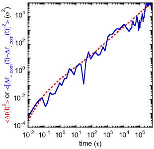
Figure 1: The two components to calculate $\Lambda/\Lambda_{NE}$ in EMD: the mean squared displacement of all ions (red dashed line) and the difference in cations’ and anion’s center of mass displacement (blue solid line). This example is from the homopolymer system at $l_{B}=0\sigma$ and $[+]/[A]=0.006$.

2.2.2 Nonequilibrium Method

We apply an external, static electric field $E$ in the x-direction. At long times, ions have a steady state drift velocity along the parallel direction of the field. The drift velocity can be calculated from

$$\langle v_{x}\rangle^{2}t^{2}=\bigl{\langle}\Delta r_{x}(t)^{2}\bigr{\rangle}_{E}-\bigl{\langle}\Delta r_{x}(t)^{2}\bigr{\rangle}_{0}=\bigl{\langle}\Delta r_{\parallel}(t)^{2}\bigr{\rangle}_{E}-\bigl{\langle}\Delta r_{\perp}(t)^{2}\bigr{\rangle}_{E}$$ (9)

where $\bigl{\langle}\bigr{\rangle}_{E}$ denotes an ensemble average in NEMD where an electric field $E$ is applied in the x-direction, $\bigl{\langle}\bigr{\rangle}_{0}$ denotes an ensemble average in EMD at zero field; $\bigl{\langle}\Delta r_{\parallel}(t)^{2}\bigr{\rangle}_{E}$ and $\bigl{\langle}\Delta r_{\perp}(t)^{2}\bigr{\rangle}_{E}$ are the directional MSDs of all ions in the parallel and perpendicular directions to the field, respectively. Instead of using the first relation that requires two simulations to be conducted, we calculated the drift velocity with the second relation as the field has no effect on the MSD in the perpendicular direction. Since the electric field is in the x-direction, $\bigl{\langle}\Delta r_{\parallel}(t)^{2}\bigr{\rangle}_{E}$ is always equivalent to $\bigl{\langle}\Delta r_{x}(t)^{2}\bigr{\rangle}_{E}$ for all systems. While $\bigl{\langle}\Delta r_{\perp}(t)^{2}\bigr{\rangle}_{E}$ is the average y- and z-directional MSD for HP systems, i.e. $\bigl{\langle}\Delta r_{\perp}(t)^{2}\bigr{\rangle}_{E}=\left(\bigl{\langle}\Delta r_{y}(t)^{2}\bigr{\rangle}_{E}+\bigl{\langle}\Delta r_{z}(t)^{2}\bigr{\rangle}_{E}\right)/2$), only the y-directional MSD (along the lamellae) is considered for BCP systems, i.e. $\bigl{\langle}\Delta r_{\perp}(t)^{2}\bigr{\rangle}_{E}=\bigl{\langle}\Delta r_{y}(t)^{2}\bigr{\rangle}_{E}$. In Figure 2, we plot $\bigl{\langle}\Delta r_{\parallel}(t)^{2}\bigr{\rangle}_{E}$ and $\bigl{\langle}\Delta r_{\perp}(t)^{2}\bigr{\rangle}_{E}$ as a function of time for an example system at various electric field strengths $E=0.05$–$0.20$, which at sufficiently long times reach log-log slopes of 2 and 1, respectively. To obtain drift velocity $\left\langle v_{x}\right\rangle$, the long time logarithmically spaced data is fitted to $a+bt^{2}$, where $a$ and $b$ are fitting parameters and $\left\langle v_{x}\right\rangle=\sqrt{b}$.

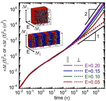
Figure 2: The directional MSD in the parallel (solid lines) and perpendicular (dashed lines) directions to the electric field with inset snapshots showing the relative directions in homopolymer and block copolymer systems. Two black lines indicate log-log slope of 1 and 2. These examples are at $l_{B}=0\sigma$ and $[+]/[A]=0.006$ and the curves shown are for the homopolymer system.

The average ion mobility $\mu$ can then be obtained by

$$\mu=\frac{\bigl{\langle}v_{x}\bigr{\rangle}}{E}$$ (10)

We are interested in $\mu$ in the linear response regime, in which the system’s behavior is not significantly disrupted from its equilibrium behavior, other than the ions’ drift in response to the field. Thus, it is necessary to check whether the drift velocity is linear with respect to $E$; in this case, value of $\mu$ does not depend on $E$. We found that our systems are well in the linear response regime across a wide range of ion concentrations and Coulomb strengths, as shown in the Supporting Information.

The molar conductivity can be directly calculated from mobilities using

$$\Lambda=\frac{\lambda}{N_{ion}}=\frac{e(\mu_{+}+\mu_{-})}{V}$$ (11)

where $\mu_{+}$ and $\mu_{-}$ are cation and anion mobilities, respectively ($\mu_{+}=\mu_{-}=\mu$ in this work). Then, $\Lambda/\Lambda_{NE}$ in NEMD is the ratio between eq 11 and eq 5, equivalent to

$$\left(\frac{\Lambda}{\Lambda_{NE}}\right)_{NEMD}=\frac{k_{B}T}{e}\left(\frac{\mu_{+}+\mu_{-}}{D_{+}+D_{-}}\right)$$ (12)

where the diffusion constants, $D_{+}$ and $D_{-}$, are calculated from eq 6 using y- and z-directional MSD for HP and y-directional MSD for BCP. We note that the MSDs used to estimate diffusion constant have one degree of freedom less than those in EMD.

2.3 Ion Cluster and Polymer Relaxation Rate

To show the ion cluster and polymer dynamics, we calculated the cluster autocorrelation function, $ACF_{cluster}$ and monomers’ self-intermediate scattering function, $S(k,t)$. We define $ACF_{cluster}=\sum_{i\neq j}C_{ij}(t)$, where $C_{ij}(t)=1$ if the beads $i$ and $j$ are in the same cluster at both time $t$ and at time $0$, and $C_{ij}(t)=0$ otherwise; the sum is over all ions and normalized to be 1 at time 0. In line with prior work, ions were considered in the same cluster if they were within $1.05\sigma$ from any other ions in the cluster, and the initial data before $0.15\tau$ was removed for better fitting (neglecting the rapid decorrelation at very short times).

We also calculated the self-intermediate scattering function by

$$S(k,t)=\frac{1}{N_{mon}}\sum_{i=1}^{N_{mon}}\bigl{\langle}e^{-i\mathbf{k}\cdotp\Delta r_{i}(t)}\bigr{\rangle}$$ (13)

where $N_{mon}$ is the number of monomer beads, $\mathbf{k}$ is the scattering vector with a magnitude of $k$. We set $k=\pi$ so that $S(k,t)$ decayed slowly enough for good fitting. Both $ACF_{cluster}$ and $S(k,t)$ were fitted to a scaled Kohlrausch-Williams-Watts (KWW) stretched exponential function, $\alpha exp[-(t/\tau^{*})^{\beta}]$, where $\alpha$, $\beta$, and $\tau^{*}$ are the fitting parameters. The ion cluster relaxation rate $\tau_{cluster}^{-1}$ or polymer relaxation rate $\tau_{polymer}^{-1}$ was then calculated by $\tau_{cluster/polymer}^{-1}=[(\tau^{*}/\beta)\Gamma(1/\beta)]^{-1}$, where $\Gamma(x)$ is the gamma function.

3 Results and Discussion

3.1 Equilibrium vs Nonequilibrium Method

As a first step to assess the accuracy and reliability of conductivity calculation from both equilibrium and nonequilibrium methods, we calculate $\Lambda/\Lambda_{NE}$ for toy systems with no Coulomb interactions between ions ($l_{B}=0\sigma$). Under such condition, ion mobility is related to the ion self-diffusion constant via the Einstein relation: $D=\mu k_{B}T/e$, which grants $\Lambda/\Lambda_{NE}=1$ regardless of salt loading. Thus, checking how close to 1 $\Lambda/\Lambda_{NE}$ is allows us to assess accuracy. In Figure 3a and b, we show $\Lambda/\Lambda_{NE}$ at $l_{B}=0\sigma$ calculated using different total amounts of simulation time in EMD and NEMD, respectively. More blocks (time windows) are averaged over for the $\Lambda/\Lambda_{NE}$ calculation as total time increases, and the error bars are the standard errors across 8 systems with different initial configurations. For EMD, the mean of $\Lambda/\Lambda_{NE}$ ranges between 0.9 and 1.1 with errors of $\pm 5$–$10\%$ when calculated using the shortest simulation time considered. The errors are $\pm 10$–$20\%$ when considering 95% confidence intervals, which are close to those reported in Ref 34. Although the errors reduce and the means converge closer to 1 as more data is averaged over, there is a persistent error even at the longest times considered here. However, $\Lambda/\Lambda_{NE}$ from NEMD is significantly faster to converge to 1 with small error compared to that from EMD. We note that, due to the concurrent calculation of $D$ and $\mu$ by assessing motion perpendicular and parallel to the field, the NEMD and EMD simulations are run for the same total time. Applying the field has negligible effect on the calculation time. The calculation of $\mu$ as a function of $E$ to ensure the system is in the linear response regime, however, is an additional step required for NEMD. This assessment did not take very long compared to the overall simulation time (see the Supporting Information). In short, the toy model results show that calculating conductivity from nonequilibrium method is rather accurate and reliable.

We then computed $\Lambda/\Lambda_{NE}$ at $l_{B}=8\sigma$ using both methods, as shown in Figure 3c and d. Unlike the toy systems where $\Lambda/\Lambda_{NE}=1$ at all ion concentrations, the result for $l_{B}=8\sigma$ is not known a priori. For EMD, the large error bars at various concentrations overlap, leading to the difference in some systems’ $\Lambda/\Lambda_{NE}$ statistically insignificant. In contrast, $\Lambda/\Lambda_{NE}$ from NEMD is consistent after $10^{5}\tau$ of simulation time with negligible error on the scale of the plot. This again shows that it is much more efficient to calculate conductivity from NEMD (it takes about 6 times longer for EMD to reach similar mean values but still with relatively large errors).

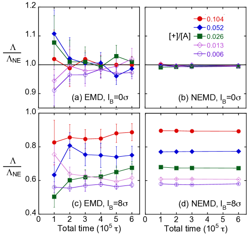
Figure 3: The degree of uncorrelated ion motion (fractional deviation of conductivity from the Nernst-Einstein equation) $\Lambda/\Lambda_{NE}$ as a function of total time of data collection (excluding the equilibration time) in homopolymers at various ion concentrations for (a),(b) $l_{B}=0\sigma$ and (c),(d) $l_{B}=8\sigma$ from EMD (a),(c) and NEMD (b),(d). The error bars are the standard errors across 8 systems with different initial configurations.

3.2 Ion Transport Properties from NEMD

After validating the conductivity calculation on a set of systems above, we now use the NEMD method to analyze ion transport in a variety of salt-doped polymer systems; specifically, we probe the effects of Coulomb and solvation interactions on ion transport by separately adjusting $l_{B}$, $S_{A\pm}$, and $S_{\pm\pm}$. We note that the mapping approach discussed in the Simulation Model section implies that $l_{B}$ and $S_{A\pm}$ are not independent (both depend on the dielectric constant of the A phase), but we vary them separately here to show the effects of these parameters. All results from the following sections are from NEMD simulations with ion conductivity directly calculated from ion mobility.

3.2.1 Effects of Coulomb strength

Figure 4a and b shows the total ion conductivity in both HP and BCP systems across a wide range of salt loading at $l_{B}=0\sigma$ and $l_{B}=8\sigma$, respectively. Both HP curves reproduce the experimentally observed nonmonotonic trend, and we find the total conductivity $\lambda$ in HPs at both Coulomb strengths peaks at a similar salt loading. The nonmonotonic relationship between conductivity and concentration apparently stems from the competition between the decrease in ion diffusion with concentration and the increase in number of ions. Prior all-atom simulations also have shown nonmonotonic conductivity behavior with relatively high $\Lambda/\Lambda_{NE}$ ($\approx 0.8$–$1.0$).³² However, in BCPs, the $\lambda$ trend varies with Coulomb strength. At $l_{B}=0\sigma$, $\lambda$ plateaus at high concentrations, whereas at $l_{B}=8\sigma$, $\lambda$ is nonmonotonic, which matches experiment.^{55, 10} We note that the conductivity of BCPs is typically smaller than that of HPs, as expected from prior work.^{55, 56} The BCP conductivity becomes similar to that of HPs at high concentration at $l_{B}=0\sigma$, which might due to ions partly mixing in the nonconducting B phase at high concentration, as shown in Figure 4c. This amount of mixing observed in our toy model at $l_{B}=0\sigma$ is not expected to be present in the BCP electrolyte systems of interest, which include both Coulomb interactions and strong selective solvation interactions.⁵⁷

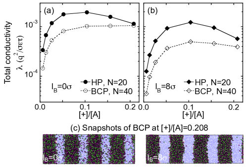
Figure 4: Ion conductivity in homopolymers (solid symbols) and block copolymers (open symbols) across a range of ion concentrations at (a) $l_{B}=0\sigma$ and (b) $l_{B}=8\sigma$. (c) Snapshots of the block copolymer systems at $[+]/[A]=0.208$.

To better understand how Coulomb strength affects ion correlations, we plotted molar conductivity $\Lambda$ and Nernst-Einstein molar conductivity $\Lambda_{NE}$ at different $l_{B}$ values in both homopolymer and block copolymer systems in Figure 5a and b, respectively (data of ion mobility and diffusion constant used to calculate conductivity are available in the Supporting Information). We find linear $\Lambda$ trends on a log scale at weak Coulomb strengths and nonlinear trends at strong Coulomb strengths. On the other hand, $\Lambda_{NE}$ as a function of ion concentration is always linear (except for the intermediate concentration regime at $l_{B}=12\sigma$, which can be attributed to the formation of larger ion clusters and will later be discussed). Linear $\Lambda_{NE}$ behavior is somewhat expected as $\Lambda_{NE}$ is mainly determined by the ion diffusion constant, which is known to be linear versus ion concentration on a log scale.³² A cross symbol is used to present an approximate result for the system at $l_{B}=12\sigma$ and $[+]/[A]=0.052$. Around this intermediate salt loading and strong Coulomb strength, the system appears to be macrophase separating. Specifically, large ion-rich and ion-poor regions are observed, and depending on whether the ion-rich region is connected from one side of the box to the other, the conductivity measurement can vary. Without assessing different box sizes to understand the overall structure of a macroscopic system, which we have not done, we cannot be confident in the bulk conductivity for this system. For the approximate result shown, we used the average from two samples where the ion-rich region is connected through the box in the parallel and perpendicular directions to the electric field, respectively (see the Supporting Information for more detail). The conductivity data from this system is consistently represented by the cross symbol throughout the work. However, in terms of the structural results, cluster relaxation rate, and polymer relaxation rate, the data do not depend significantly on the overall morphology of the ion-rich region. Thus, we have included this system as a data point in our other results.

Figure 5c summarizes the degree of uncorrelated ion motion for each system, the ratio $\Lambda/\Lambda_{NE}$. As expected, increasing Coulomb strength increases ion correlations (decreases $\Lambda/\Lambda_{NE}$). Interestingly, we find that $\Lambda/\Lambda_{NE}$ is generally lower at low ion concentrations (except for $l_{B}=0\sigma$ where it has to be $1.0$ regardless of salt loading), indicating that ion motion is more correlated at low concentrations. This contradicts the general understanding in typical electrolytes that ion motion is less correlated at low concentrations due to the screening of solvent, and is more correlated at high concentrations as large ion clusters can form.³⁴ While it is theoretically true that ion motion should become uncorrelated in the dilute limit as ions are spread far apart, we speculate that ion concentration would have to be extremely low for ion correlations to be negligible in these salt-doped polymers with strong ion-polymer and ion-ion interactions. Nonetheless, a similar trend of ion correlations has also been reported in studies of ionic liquid electrolytes⁵⁸ and nonaqueous polyelectrolytes.¹⁸ In the latter work, the contribution to conductivity from cation-anion correlated motion is more negative at lower ion concentration.¹⁸ To probe the underpinnings of these results, we analyze ion cluster and polymer relaxation rate. we found little difference in these relaxation times between HP and BCP systems, and we show only the HP results for the following sections (BCP results are shown in the Supporting Information).

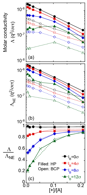
Figure 5: (a) Molar conductivity $\Lambda$, (b) Nernest-Einstein molar conductivity $\Lambda_{NE}$, and (c) degree of uncorrelated ion motion $\Lambda/\Lambda_{NE}$ in homopolymers (filled symbols) and in block copolymers (open symbols) as a function of ion concentration at $l_{B}=0\sigma$ (circles), $l_{B}=4\sigma$ (squares), $l_{B}=8\sigma$ (diamonds), and $l_{B}=12\sigma$ (triangles).

To separately study ion and polymer dynamics, we calculated cluster relaxation rate $\tau_{cluster}^{-1}$ and polymer relaxation rate $\tau_{polymer}^{-1}$ from the ion cluster autocorrelation function and monomers’ self-intermediate scattering function. These results are shown in Figure 6. We find that increasing salt loading or Coulomb strength generally lowers $\tau_{cluster}^{-1}$. However, $\tau_{cluster}^{-1}$ also decreases in the lower concentration regime at strong Coulomb strength, leading to a nonmonotonic trend. As detailed in the Supporting Information, we obtained similar nonmonotonic results using different definitions of ion cluster relaxation rates that have been reported to be related to ion conductivity.^{59, 60} On the other hand, the behavior of $\tau_{polymer}^{-1}$ with concentration is linear on a semi-log scale and is almost independent of Coulomb strength, signifying polymer dynamics mainly depend on salt loading rather than ion dynamics (until very high concentration). We also find that $\tau_{polymer}^{-1}$ is proportional to ion diffusion (in the Supporting Information) or $\Lambda_{NE}$ (Figure 5b) across various systems. This is similar to recent experimental results showing that, even in samples with inhomogeneous salt distributions, the product of lithium ion diffusion and polymer relaxation time is temperature-independent in lithium salt-doped poly(propylene glycol).⁶¹

We then normalized cluster relaxation rate by polymer relaxation rate, as shown in Figure 6c. The normalized cluster relaxation rate versus concentration is flat at $l_{B}=0\sigma$, indicating that ion dynamics is highly dependent on polymer dynamics for ions with no electrostatic interactions. However, the normalized rate reduces with increasing Coulomb strength and decreasing ion concentration for other systems. Interestingly, we find the behavior of the normalized cluster relaxation rate highly resembles that of $\Lambda/\Lambda_{NE}$, shown in Figure 5c. The result suggests that the correlation in ion motion is closely related to how long ion clusters remain intact, and is in line result from Ref. 18 where correlated cation-anion pairs were found to be able to travel longer distances with decreasing concentration despite the reduced fraction of ion pairs. The relationship between $\Lambda/\Lambda_{NE}$ and cluster relaxation rate will further be discussed in the following sections.

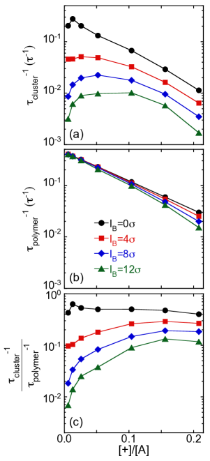
Figure 6: (a) Ion cluster relaxation rate, (b) polymer relaxation rate, and (c) their ratio (normalized ion cluster relaxation rate) as a function of ion concentration at different Coulomb strengths.

The cation-anion motion correlation behavior with concentration shown in Figure 5c is somewhat nonintuitive as one would expect that the fraction of free ions would decrease (or the cluster size to increase) as salt loading increases and that this would increase correlation in ion motion. To fully understand the trend, we analyzed a variety of structural properties of systems with different Coulomb strengths, as shown in Figure 7. Indeed, we find the fraction of free ions decreases and the average ion cluster size increases with growing ion concentration regardless of Coulomb strength (Figure 7b). Meanwhile, stronger Coulomb strength consistently makes ions more clustered at all concentrations.

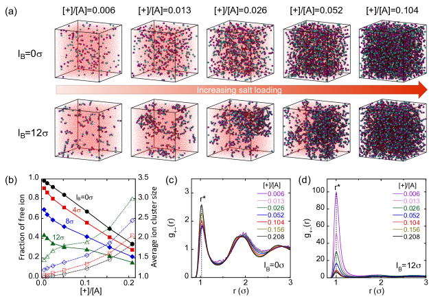
Figure 7: (a) Snapshots of homopolymer systems with various salt loading at $l_{B}=0\sigma$ (top) and $l_{B}=12\sigma$ (bottom). (b) Fraction of free ions (solid lines) and average ion cluster size (dashed lines) versus salt loading for $l_{B}=0$–$12\sigma$. (c), (d) Cation-anion radial distribution functions of homopolymer systems with various salt loading at $l_{B}=0\sigma$ and $l_{B}=12\sigma$, respectively.

We also consider ion structure by comparing the cation-anion radial distribution function, $g_{+-}(r)$, at different salt loadings and Coulomb strengths in Figure 7, along with snapshots. At $l_{B}=0\sigma$ (Figure 7c), systems at various salt loadings share a similar first peak height, denoted as $g_{+-}(r^{*})$. Only at very high concentration does $g_{+-}(r^{*})$ slightly increase, potentially due to the relative saturation of available sites for ion-monomer contact leading to some ion-ion contact. On the other hand, at $l_{B}=12\sigma$ (Figure 7d), $g_{+-}(r^{*})$ varies significantly with salt loading; specifically, the first peak height is higher at low concentrations. Figure 8 shows the height of the first peak in $g_{+-}(r)$ at different Coulomb strengths. Increasing Coulomb strength significantly increases the peak in the low concentration regime, and then the peak height plateaus after $[+]/[A]=0.1$ for all systems. Interestingly, we find the peak height, a structural measure of the amount of ion contacts, is related to cluster dynamics, specifically to the normalized cluster relaxation rate. In fact, all data points can be approximately collapsed on a single curve (inset figure) when plotting $g_{+-}(r^{*})$ versus normalized cluster relaxation rate.

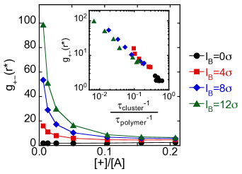
Figure 8: The first peak height of the cation-anion radial distribution function versus ion concentration at $l_{B}=0$, $4$, $8$, and $12\sigma$ with the inset showing its log-log scale relationship with the normalized cluster relaxation time.

To further understand how ion motion correlation connects to other properties, we first plotted $\Lambda/\Lambda_{NE}$ versus normalized cluster relaxation rate, as shown in Figure 9a. A strong correlation was found between the two properties across all systems regardless of Coulomb strength and ion concentration, indicating correlated ion motion is closely related to cluster dynamics. Because normalized cluster relaxation is also related to the height of the first peak of $g_{+-}(r)$, this also means that $g_{+-}(r^{*})$ predicts $\Lambda/\Lambda_{NE}$. However, the normalized cluster relaxation better explains the $\Lambda/\Lambda_{NE}$ data, especially for BCP systems whose $g_{+-}(r^{*})$ is apperently affected by ion structure near interfaces (see the Supporting Information).

One may also expect conductivity to be related to the free ion content or ion dissociation. As a result, we have also plotted $\Lambda/\Lambda_{NE}$ against fraction of free ions at different Coulomb strengths and ion concentrations. Surprisingly, there is a negative correlation between $\Lambda/\Lambda_{NE}$ and fraction of free ions as a function of ion concentration at each Coulomb strength above 0 (Figure 9b). These results show that ion motion can be less correlated when the fraction of free ions is lower (corresponding to higher concentrations and ions being more clustered), which is counterintuitive as ion agglomeration is often considered to deteriorate the ion transport. Apparently, the strength of the local ion association as quantified by $g_{+-}(r^{*})$ or normalized cluster relaxation time is a better predictor of conductivity than the fraction of free ions.

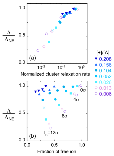
Figure 9: The degree of uncorrelated ion motion $\Lambda/\Lambda_{NE}$ as a function of (a) normalized cluster relaxation rate and (b) fraction of free ions across a range of Coulomb strengths and ion concentrations. Going from right to left for each symbol, $l_{B}=0$, $4$, $8$, then $12\sigma$.

3.2.2 Effects of ion-monomer and ion-ion solvation strength

We now probe the effects of ion-monomer solvation interaction on ion conductivity by adjusting ion-monomer solvation strength $S_{A\pm}$ and holding other variables constant. As shown in Figure 10a, ion diffusion constant decreases and $\Lambda/\Lambda_{NE}$ increases with increasing $S_{A\pm}$. In line with the results of Wheatle, Lynd, and Ganesan in Ref. 28, we also find that stronger ion-monomer interaction reduces correlated ion motion but slows polymer dynamics as well as ion diffusion. Figure 10b shows molar conductivity $\Lambda$ as a function of $S_{A\pm}$ at different ion concentrations. Increasing ion concentration increases $\Lambda/\Lambda_{NE}$ but decreases diffusion constant and $\Lambda_{NE}$. Overall, $\Lambda$ tends to peak at intermediate ion-monomer solvation strength. Significantly, we find the peak shifts to lower $S_{A\pm}$ with increasing ion concentration. As detailed in Supporting Information, at higher concentration, the detrimental effect of retarded ion diffusion becomes more influential than the conducitvity-promoting effect from reduced ion correlations. The peak shifting suggests that the potential materials design strategy of improving ion conduction by using polymers with higher dielectric constant (strengthening ion-monomer interaction) will have limited effectiveness at high salt loading. Instead, ion conductivity at high concentrations is mainly limited by the diffusion constant for the systems considered here.

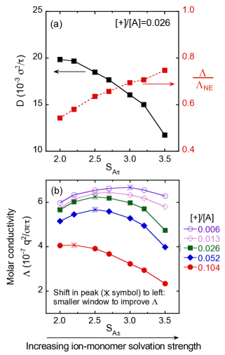
Figure 10: (a) Diffusion constant (solid line, left axis) and degree of uncorrelated ion motion (dashed line, right axis) at $[+]/[A]=0.026$ and (b) molar conductivity at various ion concentrations, as a function of ion-monomer solvation strength in homopolymers.

We also show the effects of ion-ion solvation strength $S_{\pm\pm}$ on ion transport in the Supporting Information. Nonzero $S_{\pm\pm}$ can be chosen because some ions may be bulky, polarizable molecules and thus “solvate” other ions in addition to interacting with them through the Coulomb potential. As intuitively expected, increasing $S_{\pm\pm}$ not only slows ion diffusion but also intensifies correlations in ion motion (see the Supporting Information). Thus, the molar conductivity decreases monotonically with larger $S_{\pm\pm}$. However, we postulate that this might not be the case if there were a significant size disparity between cation and anion. With small cations, their strong complexation with monomers may be the main factor acting to impede their diffusion, and we hypothesize it may be possible to mitigate this effect by including stronger interactions with anions, leading to a situation in which increasing cation-anion interactions can increase diffusion in a particular range of parameter space. We hope to explore these possible effects in future work.

The total conductivity $\lambda$ and other transport properties were measured for several selected systems with different $S_{A\pm}$ and $S_{\pm\pm}$ values across a wide range of ion concentration, as shown in Figure 11. We find that tuning ion-monomer or ion-ion interactions leads to different total conductivity versus ion concentration results: 1) Increasing $S_{A\pm}$ reduces ion motion correlation as discussed earlier, yet slows ion diffusion, especially at high concentrations. The resulting $\lambda$ remains similar with stronger ion-monomer interactions in the lower concentration regime due to competing effects between reduced diffusion constant and more uncorrelated ion motion. However, $\lambda$ decreases in the higher concentration regime. 2) Increasing $S_{\pm\pm}$ causes less uncorrelated cation-anion motion as well as slower ion diffusion; $\lambda$ shifts down to a similar extent at all concentrations.

We note that we expect the trend in HPs shown here to be similar as that in BCPs based on the results in Figure 5 that both ion diffusion and $\Lambda/\Lambda_{NE}$ trends are similar for HP and BCP systems (except the diffusion constant in BCP is always smaller). In addition, from our previous studies,^{41, 7} we have shown that the dielectric contrast $\Delta S$ (related to the difference in dielectric constant between the two blocks in BCP) is the key factor that determines how ion transport properties in BCPs deviate from those in HPs. Thus, we also have tested the impact of $\Delta S$ on ion dynamics in this work, as shown in the Supporting Information. In line with Ref. 7, we show that $\Lambda/\Lambda_{NE}$ is nearly independent of $\Delta S$ and ion diffusion constant decreases with increasing $\Delta S$.

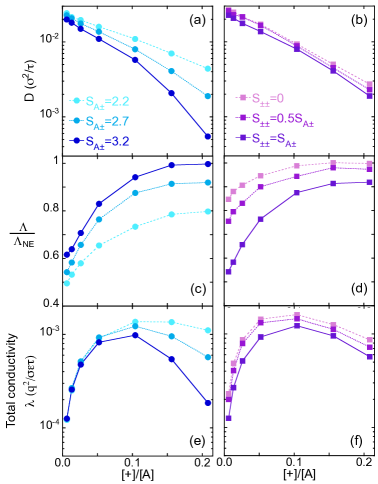
Figure 11: (a),(b) Diffusion constant, (c),(d) degree of uncorrelated ion motion $\Lambda/\Lambda_{NE}$, and (e),(f) ion conductivity as a function of ion concentration at various ion-A interactions (a),(c),(e) and ion-ion interactions (b),(d),(f).

3.2.3 Ion Correlations in Low and High Concentration Regimes

Finally, having observed the dependence of ion correlations on salt loading, we plotted molar conductivity of all systems considered above (including systems with various $l_{B}$, $S_{A\pm}$, and $S_{\pm\pm}$) as a function of ion diffusion constant separately at high concentrations ($[+]/[A]>0.1$) and at low concentrations ($[+]/[A]<0.1$), as shown in Figure 12a and b, respectively. At high concentrations, regardless of changes in interactions, we find molar conductivity can be well predicted by diffusion constant since $\Lambda/\Lambda_{NE}$ is close to 1. On the other hand, at low concentrations, $\Lambda/\Lambda_{NE}$ ranges from $0.2-1.0$ and molar conductivity is not always well predicted by the diffusion constant. Out another way, this means that the Nernst-Einstein equation tends to be a better approximation at high concentrations in polymer electrolytes, whereas at low concentrations, ion conductivity is more likely to deviate from Nernst-Einstein limit due to the cation-anion motion correlation. As discussed earlier, this is in contrast to typical electrolytes where Nernst-Einstein equation is often expected to be more applicable at low ion concentrations.

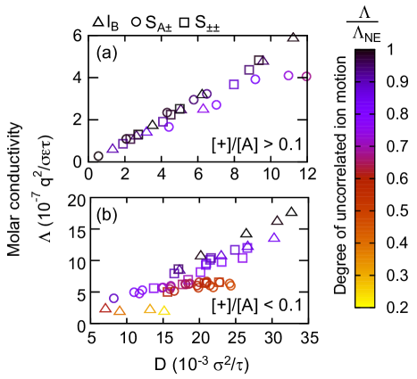
Figure 12: Molar conductivity as a function of ion diffusion constant at (a) high and (b) low concentration. The color of the data points corresponds to the degree of uncorrelated ion motion as indicated by the color bar. Points with different shapes represent systems with varying Coulomb strength (triangles), ion-monomer solvation strength (circles), and ion-ion solvation strength (squares).

4 Conclusions

We perform MD simulations with an applied electric field to calculate ion conductivity directly from ion mobility. By assessing a toy model where no electrostatic potential exists between ions, we show that it is more accurate and efficient to calculate ion conductivity and ion correlations from the nonequilibrium method than the typical use of fluctuation dissipation relationships in equilibrium simulations. After validating the accuracy, we use this method to further probe the effects of ion-ion and ion-monomer interactions on ion transport across a wide range of ion concentrations with our recently-developed model (with a $1/r^{4}$ potential form to represent ion solvation).

We find that cation-anion motion is more correlated at lower concentrations when other variables are held constant. We demonstrate that this phenomenon is due to the slower ion cluster relaxation rate at low concentrations rather than the static spatial state of ion aggregation or the fraction of free ions. Two takeaways from these results are: 1) In salt-doped polymer systems, the Nernst-Einstein equation is more applicable at higher concentrations, which in contrast to typical electrolytes where correlation in cation-anion motion is often expected to be reduced at low ion concentrations. 2) The number of free ions, which is often expected to be related to ion conductivity, does not fully explain the dynamic ion motion correlations or conductivity.

We consider systems with various ion-monomer and ion-ion solvation strengths. Optimal molar conductivity can be obtained by tuning ion-monomer solvation strength. However, we show that the window to improve ion conductivity by increasing dielectric constant is smaller at higher concentrations. Stronger ion-monomer interactions causes competing diffusion and ion correlation effects at low concentrations but significantly reduces ion conductivity at high concentrations due to the dominant decrease in the diffusion constant. On the other hand, increasing ion-ion interactions impedes ion conduction regardless of ion concentration.

Finally, at all ion-monomer and ion-ion interactions considered in this work, ion conductivity was found well predicted by ion diffusion at higher concentrations. On the contrary, the degree of uncorrelated ion motion cannot be neglected to accurately calculate ion conductivity at low concentrations. From an experimental standpoint, our results suggest that analysis such as electrophoretic NMR (eNMR)⁶² or broadband dielectric spectroscopy (BDS)⁹ is needed to probe the actual correlations of ion motion rather than pulsed field gradient NMR which measures diffusion of different species. In addition, scaling conductivity or diffusion constant based on fraction of free/dissociated ions in these systems may not be appropriate.^{11, 63} By elucidating how these key factors affect ion conductivity and correlations, we hope to provide insight on how to optimize ion conduction in future materials.

5 Acknowledgements

We thank Venkat Ganesan for for helpful discussions regarding the conductivity calculation. This material is based upon work supported by the U.S. Department of Energy, Office of Science, Office of Basic Energy Sciences, under Award No. DE-SC0014209 (K.-H.S.). Additionally, this material is based upon work supported by the National Science Foundation under Grant No. 1454343 (L.M.H.). We acknowledge the support and high performance computing (HPC) resources from the Ohio Supercomputing Center.⁶⁴

References

- Ketkar et al. 2019 Ketkar, P. M.; Shen, K.-H.; Hall, L. M.; Epps, T. H. Charging toward improved lithium-ion polymer electrolytes: exploiting synergistic experimental and computational approaches to facilitate materials design. Molecular Systems Design & Engineering 2019, 4, 223–238
- Miller III et al. 2017 Miller III, T. F.; Wang, Z.-G.; Coates, G. W.; Balsara, N. P. Designing polymer electrolytes for safe and high capacity rechargeable lithium batteries. Accounts of Chemical Research 2017, 50, 590–593
- Ganesan et al. 2012 Ganesan, V.; Pyramitsyn, V.; Bertoni, C.; Shah, M. Mechanisms underlying ion transport in lamellar block copolymer membranes. ACS Macro Letters 2012, 1, 513–518
- Webb et al. 2015 Webb, M. A.; Jung, Y.; Pesko, D. M.; Savoie, B. M.; Yamamoto, U.; Coates, G. W.; Balsara, N. P.; Wang, Z.-G.; Miller III, T. F. Systematic computational and experimental investigation of lithium-ion transport mechanisms in polyester-based polymer electrolytes. ACS central science 2015, 1, 198–205
- Cheng et al. 2018 Cheng, Y.; Yang, J.; Hung, J.-H.; Patra, T. K.; Simmons, D. S. Design rules for highly conductive polymeric ionic liquids from molecular dynamics simulations. Macromolecules 2018, 51, 6630–6644
- Shen et al. 2018 Shen, K.-H.; Brown, J. R.; Hall, L. M. Diffusion in lamellae, cylinders, and double gyroid block copolymer nanostructures. ACS Macro Letters 2018, 7, 1092–1098
- Seo et al. 2019 Seo, Y.; Shen, K.-H.; Brown, J. R.; Hall, L. M. Role of solvation on diffusion of ions in diblock copolymers: understanding the molecular weight effect through modeling. Journal of the American Chemical Society 2019, 141, 18455–18466
- Gainaru et al. 2016 Gainaru, C.; Stacy, E. W.; Bocharova, V.; Gobet, M.; Holt, A. P.; Saito, T.; Greenbaum, S.; Sokolov, A. P. Mechanism of conductivity relaxation in liquid and polymeric electrolytes: Direct link between conductivity and diffusivity. The Journal of Physical Chemistry B 2016, 120, 11074–11083
- Stacy et al. 2018 Stacy, E. W.; Gainaru, C. P.; Gobet, M.; Wojnarowska, Z.; Bocharova, V.; Greenbaum, S. G.; Sokolov, A. P. Fundamental limitations of ionic conductivity in polymerized ionic liquids. Macromolecules 2018, 51, 8637–8645
- Galluzzo et al. 2020 Galluzzo, M. D.; Loo, W. S.; Wang, A. A.; Walton, A.; Maslyn, J. A.; Balsara, N. P. Measurement of Three Transport Coefficients and the Thermodynamic Factor in Block Copolymer Electrolytes with Different Morphologies. The Journal of Physical Chemistry B 2020, DOI: 10.1021/acs.jpcb.9b11066
- Colby et al. 1997 Colby, R. H.; Boris, D. C.; Krause, W. E.; Tan, J. S. Polyelectrolyte conductivity. Journal of Polymer Science Part B: Polymer Physics 1997, 35, 2951–2960
- Timachova et al. 2015 Timachova, K.; Watanabe, H.; Balsara, N. P. Effect of molecular weight and salt concentration on ion transport and the transference number in polymer electrolytes. Macromolecules 2015, 48, 7882–7888
- Buss et al. 2017 Buss, H. G.; Chan, S. Y.; Lynd, N. A.; McCloskey, B. D. Nonaqueous polyelectrolyte solutions as liquid electrolytes with high lithium ion transference number and conductivity. ACS Energy Letters 2017, 2, 481–487
- Krachkovskiy et al. 2017 Krachkovskiy, S. A.; Bazak, J. D.; Fraser, S.; Halalay, I. C.; Goward, G. R. Determination of Mass Transfer Parameters and Ionic Association of LiPF6: Organic Carbonates Solutions. Journal of The Electrochemical Society 2017, 164, A912–A916
- Gouverneur et al. 2015 Gouverneur, M.; Kopp, J.; van Wüllen, L.; Schönhoff, M. Direct determination of ionic transference numbers in ionic liquids by electrophoretic NMR. Physical Chemistry Chemical Physics 2015, 17, 30680–30686
- Rosenwinkel and Schönhoff 2019 Rosenwinkel, M. P.; Schönhoff, M. Lithium Transference Numbers in PEO/LiTFSA Electrolytes Determined by Electrophoretic NMR. Journal of The Electrochemical Society 2019, 166, A1977–A1983
- Diederichsen et al. 2018 Diederichsen, K. M.; Fong, K. D.; Terrell, R. C.; Persson, K. A.; McCloskey, B. D. Investigation of solvent type and salt addition in high transference number nonaqueous polyelectrolyte solutions for lithium ion batteries. Macromolecules 2018, 51, 8761–8771
- Fong et al. 2019 Fong, K. D.; Self, J.; Diederichsen, K. M.; Wood, B. M.; McCloskey, B. D.; Persson, K. A. Ion Transport and the True Transference Number in Nonaqueous Polyelectrolyte Solutions for Lithium Ion Batteries. ACS Central Science 2019, 5, 1250–1260
- Lonergan et al. 1995 Lonergan, M. C.; Shriver, D. F.; Ratner, M. A. Polymer electrolytes: The importance of ion-ion interactions in diffusion dominated behavior. Electrochimica acta 1995, 40, 2041–2048
- Payne et al. 1995 Payne, V. A.; Lonergan, M. C.; Forsyth, M.; Ratner, M. A.; Shriver, D. F.; de Leeuw, S. W.; Perram, J. W. Simulations of structure and transport in polymer electrolytes. Solid State Ionics 1995, 81, 171–181
- Harris 2010 Harris, K. R. Relations between the fractional Stokes- Einstein and Nernst- Einstein equations and velocity correlation coefficients in ionic liquids and molten salts. The Journal of Physical Chemistry B 2010, 114, 9572–9577
- Pesko et al. 2017 Pesko, D. M.; Timachova, K.; Bhattacharya, R.; Smith, M. C.; Villaluenga, I.; Newman, J.; Balsara, N. P. Negative transference numbers in poly (ethylene oxide)-based electrolytes. Journal of The Electrochemical Society 2017, 164, E3569–E3575
- Gouverneur et al. 2018 Gouverneur, M.; Schmidt, F.; Schönhoff, M. Negative effective Li transference numbers in Li salt/ionic liquid mixtures: does Li drift in the "Wrong" direction? Physical Chemistry Chemical Physics 2018, 20, 7470–7478
- Villaluenga et al. 2018 Villaluenga, I.; Pesko, D. M.; Timachova, K.; Feng, Z.; Newman, J.; Srinivasan, V.; Balsara, N. P. Negative Stefan-Maxwell Diffusion Coefficients and Complete Electrochemical Transport Characterization of Homopolymer and Block Copolymer Electrolytes. Journal of The Electrochemical Society 2018, 165, A2766–A2773
- Molinari et al. 2019 Molinari, N.; Mailoa, J. P.; Kozinsky, B. General Trend of a Negative Li Effective Charge in Ionic Liquid Electrolytes. The Journal of Physical Chemistry Letters 2019, 10, 2313–2319
- Molinari et al. 2019 Molinari, N.; Mailoa, J. P.; Craig, N.; Christensen, J.; Kozinsky, B. Transport anomalies emerging from strong correlation in ionic liquid electrolytes. Journal of Power Sources 2019, 428, 27–36
- Wheatle et al. 2017 Wheatle, B. K.; Keith, J. R.; Mogurampelly, S.; Lynd, N. A.; Ganesan, V. Influence of dielectric constant on ionic transport in polyether-based electrolytes. ACS Macro Letters 2017, 6, 1362–1367
- Wheatle et al. 2018 Wheatle, B. K.; Lynd, N. A.; Ganesan, V. Effect of Polymer Polarity on Ion Transport: A Competition between Ion Aggregation and Polymer Segmental Dynamics. ACS Macro Letters 2018, 7, 1149–1154
- Wheatle et al. 2019 Wheatle, B. K.; Fuentes, E. F.; Lynd, N. A.; Ganesan, V. Influence of Host Polarity on Correlating Salt Concentration, Molecular Weight, and Molar Conductivity in Polymer Electrolytes. ACS Macro Letters 2019, 8, 888–892
- Kashyap et al. 2011 Kashyap, H. K.; Annapureddy, H. V.; Raineri, F. O.; Margulis, C. J. How is charge transport different in ionic liquids and electrolyte solutions? The Journal of Physical Chemistry B 2011, 115, 13212–13221
- Zhang et al. 2019 Zhang, Z.; Wheatle, B. K.; Krajniak, J.; Keith, J. R.; Ganesan, V. Ion Mobilities, Transference Numbers, and Inverse Haven Ratios of Polymeric Ionic Liquids. ACS Macro Letters 2019, 9, 84–89
- Borodin and Smith 2006 Borodin, O.; Smith, G. D. Mechanism of ion transport in amorphous poly (ethylene oxide)/LiTFSI from molecular dynamics simulations. Macromolecules 2006, 39, 1620–1629
- Wheatle et al. 2020 Wheatle, B. K.; Lynd, N. A.; Ganesan, V. Effect of Host Incompatibility and Polarity Contrast on Ion Transport in Ternary Polymer-Polymer-Salt Blend Electrolytes. Macromolecules 2020, DOI: 10.1021/acs.macromol.9b02510
- France-Lanord and Grossman 2019 France-Lanord, A.; Grossman, J. C. Correlations from ion pairing and the Nernst-Einstein equation. Physical Review Letters 2019, 122, 136001
- Ting et al. 2015 Ting, C. L.; Stevens, M. J.; Frischknecht, A. L. Structure and dynamics of coarse-grained ionomer melts in an external electric field. Macromolecules 2015, 48, 809–818
- Weyman et al. 2018 Weyman, A.; Bier, M.; Holm, C.; Smiatek, J. Microphase separation and the formation of ion conductivity channels in poly (ionic liquid) s: A coarse-grained molecular dynamics study. The Journal of Chemical Physics 2018, 148, 193824
- Alshammasi and Escobedo 2018 Alshammasi, M. S.; Escobedo, F. A. Correlation between Ionic Mobility and Microstructure in Block Copolymers. A Coarse-Grained Modeling Study. Macromolecules 2018, 51, 9213–9221
- Wheeler and Newman 2004 Wheeler, D. R.; Newman, J. Molecular dynamics simulations of multicomponent diffusion. 2. Nonequilibrium method. The Journal of Physical Chemistry B 2004, 108, 18362–18367
- Wheeler and Newman 2004 Wheeler, D. R.; Newman, J. Molecular dynamics simulations of multicomponent diffusion. 1. Equilibrium method. The Journal of Physical Chemistry B 2004, 108, 18353–18361
- Liu and Maginn 2011 Liu, H.; Maginn, E. A molecular dynamics investigation of the structural and dynamic properties of the ionic liquid 1-n-butyl-3-methylimidazolium bis (trifluoromethanesulfonyl) imide. The Journal of Chemical Physics 2011, 135, 124507
- Brown et al. 2018 Brown, J. R.; Seo, Y.; Hall, L. M. Ion correlation effects in salt-doped block copolymers. Physical Review Letters 2018, 120, 127801
- Grest et al. 1996 Grest, G. S.; Lacasse, M.-D.; Kremer, K.; Gupta, A. M. Efficient continuum model for simulating polymer blends and copolymers. The Journal of Chemical Physics 1996, 105, 10583–10594
- Nakamura et al. 2011 Nakamura, I.; Balsara, N. P.; Wang, Z.-G. Thermodynamics of ion-containing polymer blends and block copolymers. Physical Review Letters 2011, 107, 198301
- Porter and Boyd 1971 Porter, C.; Boyd, R. A dielectric study of the effects of melting on molecular relaxation in poly (ethylene oxide) and polyoxymethylene. Macromolecules 1971, 4, 589–594
- Gray et al. 1989 Gray, F.; Vincent, C.; Kent, M. A Study of the dielectric properties of the polymer electrolyte PEO-LiClO4 over a composition range using time domain spectroscopy. Journal of Polymer Science Part B: Polymer Physics 1989, 27, 2011–2022
- Mao et al. 2000 Mao, G.; Saboungi, M.-L.; Price, D. L.; Armand, M. B.; Howells, W. Structure of liquid PEO-LiTFSI electrolyte. Physical Review Letters 2000, 84, 5536
- Hegde et al. 2016 Hegde, V.-J.; Gallot-Lavallée, O.; Heux, L. Dielectric study of Polycaprolactone: A biodegradable polymer. 2016 IEEE International Conference on Dielectrics (ICD). 2016; pp 293–296
- Roberts and Von Hippel 1946 Roberts, S.; Von Hippel, A. A new method for measuring dielectric constant and loss in the range of centimeter waves. Journal of Applied Physics 1946, 17, 610–616
- Yano and Wada 1971 Yano, O.; Wada, Y. Dynamic mechanical and dielectric relaxations of polystyrene below the glass temperature. Journal of Polymer Science Part A-2: Polymer Physics 1971, 9, 669–686
- Plimpton 1995 Plimpton, S. Fast parallel algorithms for short-range molecular dynamics. Journal of Computational Physics 1995, 117, 1–19
- Humphrey et al. 1996 Humphrey, W.; Dalke, A.; Schulten, K. VMD: visual molecular dynamics. Journal of Molecular Graphics 1996, 14, 33–38
- Seo et al. 2017 Seo, Y.; Brown, J. R.; Hall, L. M. Diffusion of selective penetrants in interfacially modified block copolymers from molecular dynamics simulations. ACS Macro Letters 2017, 6, 375–380
- Sampath and Hall 2018 Sampath, J.; Hall, L. M. Impact of ion content and electric field on mechanical properties of coarse-grained ionomers. The Journal of Chemical Physics 2018, 149, 163313
- Hansen and McDonald 2013 Hansen, J.-P.; McDonald, I. R. Theory of simple liquids: with applications to soft matter; Academic Press, 2013
- Chintapalli et al. 2016 Chintapalli, M.; Le, T. N.; Venkatesan, N. R.; Mackay, N. G.; Rojas, A. A.; Thelen, J. L.; Chen, X. C.; Devaux, D.; Balsara, N. P. Structure and ionic conductivity of polystyrene-block-poly (ethylene oxide) electrolytes in the high salt concentration limit. Macromolecules 2016, 49, 1770–1780
- Singh et al. 2007 Singh, M.; Odusanya, O.; Wilmes, G. M.; Eitouni, H. B.; Gomez, E. D.; Patel, A. J.; Chen, V. L.; Park, M. J.; Fragouli, P.; Iatrou, H.; Hadjichristidis, N.; Cookson, D.; Balsara, N. P. Effect of molecular weight on the mechanical and electrical properties of block copolymer electrolytes. Macromolecules 2007, 40, 4578–4585
- Gomez et al. 2009 Gomez, E. D.; Panday, A.; Feng, E. H.; Chen, V.; Stone, G. M.; Minor, A. M.; Kisielowski, C.; Downing, K. H.; Borodin, O.; Smith, G. D.; Balsara, N. P. Effect of ion distribution on conductivity of block copolymer electrolytes. Nano Letters 2009, 9, 1212–1216
- Haskins et al. 2014 Haskins, J. B.; Bennett, W. R.; Wu, J. J.; Hernández, D. M.; Borodin, O.; Monk, J. D.; Bauschlicher Jr, C. W.; Lawson, J. W. Computational and experimental investigation of Li-doped ionic liquid electrolytes:[pyr14][TFSI],[pyr13][FSI], and [EMIM][BF4]. The Journal of Physical Chemistry B 2014, 118, 11295–11309
- Zhao et al. 2009 Zhao, W.; Leroy, F.; Heggen, B.; Zahn, S.; Kirchner, B.; Balasubramanian, S.; Müller-Plathe, F. Are there stable ion-pairs in room-temperature ionic liquids? Molecular dynamics simulations of 1-n-butyl-3-methylimidazolium hexafluorophosphate. Journal of the American Chemical Society 2009, 131, 15825–15833
- Zhang and Maginn 2015 Zhang, Y.; Maginn, E. J. Direct correlation between ionic liquid transport properties and ion pair lifetimes: a molecular dynamics study. The Journal of Physical Chemistry Letters 2015, 6, 700–705
- Becher et al. 2019 Becher, M.; Becker, S.; Hecht, L.; Vogel, M. From Local to Diffusive Dynamics in Polymer Electrolytes: NMR Studies on Coupling of Polymer and Ion Dynamics across Length and Time Scales. Macromolecules 2019,
- Zhang and Madsen 2014 Zhang, Z.; Madsen, L. A. Observation of separate cation and anion electrophoretic mobilities in pure ionic liquids. The Journal of Chemical Physics 2014, 140, 084204
- Duluard et al. 2008 Duluard, S.; Grondin, J.; Bruneel, J.-L.; Pianet, I.; Grélard, A.; Campet, G.; Delville, M.-H.; Lassègues, J.-C. Lithium solvation and diffusion in the 1-butyl-3-methylimidazolium bis (trifluoromethanesulfonyl) imide ionic liquid. Journal of Raman Spectroscopy 2008, 39, 627–632
- Center 1987 Center, O. S. Ohio Supercomputer Center. 1987; \urlhttp://osc.edu/ark:/19495/f5s1ph73